Image Augmentation Is All You Need:
Regularizing Deep Reinforcement Learning
from Pixels
Abstract
We propose a simple data augmentation technique that can be applied to standard model-free reinforcement learning algorithms, enabling robust learning directly from pixels without the need for auxiliary losses or pre-training. The approach leverages input perturbations commonly used in computer vision tasks to transform input examples, as well as regularizing the value function and policy. Existing model-free approaches, such as Soft Actor-Critic (SAC) [22], are not able to train deep networks effectively from image pixels. However, the addition of our augmentation method dramatically improves SAC’s performance, enabling it to reach state-of-the-art performance on the DeepMind control suite, surpassing model-based [23, 38, 24] methods and recently proposed contrastive learning [50]. Our approach, which we dub DrQ: Data-regularized Q, can be combined with any model-free reinforcement learning algorithm. We further demonstrate this by applying it to DQN [43] and significantly improve its data-efficiency on the Atari 100k [31] benchmark. An implementation can be found at https://sites.google.com/view/data-regularized-q.
1 Introduction
Sample-efficient deep reinforcement learning (RL) algorithms capable of directly training from image pixels would open up many real-world applications in control and robotics. However, simultaneously training a convolutional encoder alongside a policy network is challenging when given limited environment interaction, strong correlation between samples and a typically sparse reward signal. Naive attempts to use a large capacity encoder result in severe over-fitting (see Figure 1a) and smaller encoders produce impoverished representations that limit task performance.
Limited supervision is a common problem across AI and a number of approaches are adopted: (i) pre-training with self-supervised learning (SSL), followed by standard supervised learning; (ii) supervised learning with an additional auxiliary loss and (iii) supervised learning with data augmentation. SSL approaches are highly effective in the large data regime, e.g. in domains such as vision [7, 25] and NLP [12, 13] where large (unlabeled) datasets are readily available. However, in sample-efficient RL, training data is more limited due to restricted interaction between the agent and the environment, resulting in only – transitions from a few hundred trajectories. While there are concurrent efforts exploring SSL in the RL context [50], in this paper we take a different approach, focusing on data augmentation.
A wide range of auxiliary loss functions have been proposed to augment supervised objectives, e.g. weight regularization, noise injection [28], or various forms of auto-encoder [34]. In RL, reconstruction objectives [29, 60] or alternate tasks are often used [16]. However, these objectives are unrelated to the task at hand, thus have no guarantee of inducing an appropriate representation for the policy network.
Data augmentation methods have proven highly effective in vision and speech domains, where output-invariant perturbations can easily be applied to the labeled input examples. Surprisingly, data augmentation has received relatively little attention in the RL community, and this is the focus of this paper. The key idea is to use standard image transformations to peturb input observations, as well as regularizing the -function learned by the critic so that different transformations of the same input image have similar -function values. No further modifications to standard actor-critic algorithms are required, obviating the need for additional losses, e.g. based on auto-encoders [60], dynamics models [24, 23], or contrastive loss terms [50].
The paper makes the following contributions: (i) we demonstrate how straightforward image augmentation, applied to pixel observations, greatly reduces over-fitting in sample-efficient RL settings, without requiring any change to the underlying RL algorithm. (ii) exploiting MDP structure, we introduce two simple mechanisms for regularizing the value function which are generally applicable in the context of model-free off-policy RL. (iii) Combined with vanilla SAC [22] and using hyper-parameters fixed across all tasks, the overall approach obtains state-of-the-art performance on the DeepMind control suite [51]. (iv) Combined with a DQN-like agent, the approach also obtains state-of-the-art performance on the Atari 100k benchmark. (v) It is thus the first effective approach able to train directly from pixels without the need for unsupervised auxiliary losses or a world model. (vi) We also provide a PyTorch implementation of the approach combined with SAC and DQN.


2 Background
Reinforcement Learning from Images We formulate image-based control as an infinite-horizon partially observable Markov decision process (POMDP) [6, 30]. An POMDP can be described as the tuple , where is the high-dimensional observation space (image pixels), is the action space, the transition dynamics capture the probability distribution over the next observation given the history of previous observations and current action , is the reward function that maps the current observation and action to a reward , and is a discount factor. Per common practice [43], throughout the paper the POMDP is converted into an MDP [6] by stacking several consecutive image observations into a state . For simplicity we redefine the transition dynamics and the reward function . We then aim to find a policy that maximizes the cumulative discounted return .
Soft Actor-Critic The Soft Actor-Critic (SAC) [22] learns a state-action value function , a stochastic policy and a temperature to find an optimal policy for an MDP by optimizing a -discounted maximum-entropy objective [62]. is used generically to denote the parameters updated through training in each part of the model.
Deep Q-learning DQN [43] also learns a convolutional neural net to approximate Q-function over states and actions. The main difference is that DQN operates on discrete actions spaces, thus the policy can be directly inferred from Q-values. In practice, the standard version of DQN is frequently combined with a set of refinements that improve performance and training stability, commonly known as Rainbow [53]. For simplicity, the rest of the paper describes a generic actor-critic algorithm rather than DQN or SAC in particular. Further background on DQN and SAC can be found in Appendix A.
3 Sample Efficient Reinforcement Learning from Pixels
This work focuses on the data-efficient regime, seeking to optimize performance given limited environment interaction. In Figure 1a we show a motivating experiment that demonstrates over-fitting to be a significant issue in this scenario. Using three tasks from the DeepMind control suite [51], SAC [22] is trained with the same policy network architecture but using different image encoder architectures, taken from the following RL approaches: NatureDQN [43], Dreamer [23], Impala [17], SAC-AE [60] (also used in CURL [50]), and D4PG [4]. The encoders vary significantly in their capacity, with parameter counts ranging from 220k to 2.4M. The curves show that performance decreases as parameter count increases, a clear indication of over-fitting.
3.1 Image Augmentation
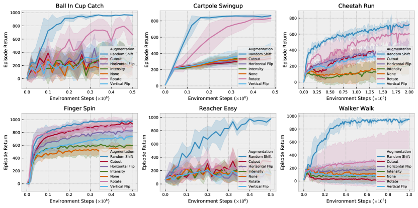
A range of successful image augmentation techniques to counter over-fitting have been developed in computer vision [8, 9, 48, 35, 7]. These apply transformations to the input image for which the task labels are invariant, e.g. for object recognition tasks, image flips and rotations do not alter the semantic label. However, tasks in RL differ significantly from those in vision and in many cases the reward would not be preserved by these transformations. We examine several common image transformations from [7] in Appendix E and conclude that random shifts strike a good balance between simplicity and performance, we therefore limit our choice of augmentation to this transformation.
Figure 1b shows the results of this augmentation applied during SAC training. We apply data augmentation only to the images sampled from the replay buffer and not for samples collection procedure. The images from the DeepMind control suite are . We pad each side by pixels (by repeating boundary pixels) and then select a random crop, yielding the original image shifted by pixels. This procedure is repeated every time an image is sampled from the replay buffer. The plots show overfitting is greatly reduced, closing the performance gap between the encoder architectures. These random shifts alone enable SAC to achieve competitive absolute performance, without the need for auxiliary losses.
3.2 Optimality Invariant Image Transformations
While the image augmentation described above is effective, it does not fully exploit the MDP structure inherent in RL tasks. We now introduce a general framework for regularizing the value function through transformations of the input state. For a given task, we define an optimality invariant state transformation as a mapping that preserves the -values
where are the parameters of , drawn from the set of all possible parameters . One example of such transformations are the random image translations successfully applied in the previous section.
For every state, the transformations allow the generation of several surrogate states with the same -values, thus providing a mechanism to reduce the variance of -function estimation. In particular, for an arbitrary distribution of states and policy , instead of using a single sample , estimation of the following expectation
we can instead generate samples via random transformations and obtain an estimate with lower variance
This suggests two distinct ways to regularize -function. First, we use the data augmentation to compute the target values for every transition tuple as
| (1) |
where corresponds to a transformation parameter of . Then the Q-function is updated using these targets through an SGD update using learning rate
| (2) |
In tandem, we note that the same target from Equation 1 can be used for different augmentations of , resulting in the second regularization approach
| (3) |
When both regularization methods are used, and are drawn independently.
3.3 Our approach: Data-regularized Q (DrQ)
Our approach, DrQ, is the union of the three separate regularization mechanisms introduced above:
-
1.
transformations of the input image (Section 3.1).
-
2.
averaging the target over K image transformations (Equation 1).
-
3.
averaging the function itself over M image transformations (Equation 3).
Algorithm 1 details how they are incorporated into a generic pixel-based off-policy actor-critic algorithm. If [K=1,M=1] then DrQ reverts to image transformations alone, this makes applying DrQ to any model-free RL algorithm straightforward as it does not require any modifications to the algorithm itself. Note that DrQ [K=1,M=1] also exactly recovers the concurrent work of RAD [36], up to a particular choice of hyper-parameters and data augmentation type.
For the experiments in this paper, we pair DrQ with SAC [22] and DQN [43], popular model-free algorithms for control in continuous and discrete action spaces respectively. We select image shifts as the class of image transformations , with , as explained in Section 3.1. For target Q and Q augmentation we use [K=2,M=2] respectively. Figure 2 shows DrQ and ablated versions, demonstrating clear gains over unaugmented SAC. A more extensive ablation can be found in Appendix F.

Black: unmodified off-policy actor-critic.
Orange: image transformation.
Green: target augmentation.
Blue: augmentation.
4 Experiments
In this section we evaluate our algorithm (DrQ) on the two commonly used benchmarks based on the DeepMind control suite [51], namely the PlaNet [24] and Dreamer [23] setups. Throughout these experiments all hyper-parameters of the algorithm are kept fixed: the actor and critic neural networks are trained using the Adam optimizer [33] with default parameters and a mini-batch size of . For SAC, the soft target update rate is , initial temperature is , and target network and the actor updates are made every critic updates (as in [60]). We use the image encoder architecture from SAC-AE [60] and follow their training procedure. The full set of parameters is in Appendix B.
| 500k step scores | DrQ (Ours) | CURL | PlaNet | SAC-AE | SLAC | SAC State |
|---|---|---|---|---|---|---|
| Finger Spin | 938103 | 874151 | 71840 | 914107 | 771203 | 92743 |
| Cartpole Swingup | 86810 | 86130 | 78746 | 730152 | - | 8707 |
| Reacher Easy | 94271 | 90494 | 588471 | 601135 | - | 9755 |
| Cheetah Run | 66096 | 50091 | 56821 | 54450 | 62974 | 77260 |
| Walker Walk | 92145 | 90656 | 478164 | 85882 | 86597 | 9648 |
| Ball In Cup Catch | 9639 | 95813 | 93943 | 810121 | 9594 | 9796 |
| 100k step scores | ||||||
| Finger Spin | 901104 | 779108 | 56077 | 747130 | 680130 | 67276 |
| Cartpole Swingup | 75992 | 592170 | 56373 | 27638 | - | 81245 |
| Reacher Easy | 601213 | 517113 | 82174 | 225164 | - | 919123 |
| Cheetah Run | 34467 | 30748 | 165123 | 252173 | 39147∗ | 22895 |
| Walker Walk | 612164 | 344132 | 22143 | 39558 | 42874 | 604317 |
| Ball In Cup Catch | 91353 | 772241 | 710217 | 338196 | 607173 | 95726 |
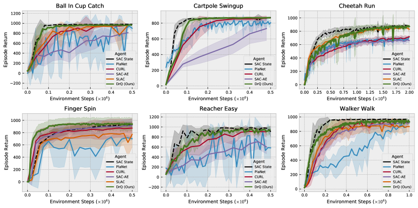
Following [27], the models are trained using different seeds; for every seed the mean episode returns are computed every environment steps, averaging over episodes. All figures plot the mean performance over the seeds, together with 1 standard deviation shading. We compare our DrQ approach to leading model-free and model-based approaches: PlaNet [24], SAC-AE [60], SLAC [38], CURL [50] and Dreamer [23]. The comparisons use the results provided by the authors of the corresponding papers.
4.1 DeepMind Control Suite Experiments
PlaNet Benchmark [24] consists of six challenging control tasks from [51] with different traits. The benchmark specifies a different action-repeat hyper-parameter for each of the six tasks111This means the number of training observations is a fraction of the environment steps (e.g. an episode of steps with action-repeat results in training observations).. Following common practice [24, 38, 60, 43], we report the performance using true environment steps, thus are invariant to the action-repeat hyper-parameter. Aside from action-repeat, all other hyper-parameters of our algorithm are fixed across the six tasks, using the values previously detailed.
Figure 3 compares DrQ [K=2,M=2] to PlaNet [24], SAC-AE [60], CURL [50], SLAC [38], and an upper bound performance provided by SAC [22] that directly learns from internal states. We use the version of SLAC that performs one gradient update per an environment step to ensure a fair comparison to other approaches. DrQ achieves state-of-the-art performance on this benchmark on all the tasks, despite being much simpler than other methods. Furthermore, since DrQ does not learn a model [24, 38] or any auxiliary tasks [50], the wall clock time also compares favorably to the other methods. In Table 1 we also compare performance given at a fixed number of environment interactions (e.g. k and k). Furthermore, in Appendix G we demonstrate that DrQ is robust to significant changes in hyper-parameter settings.
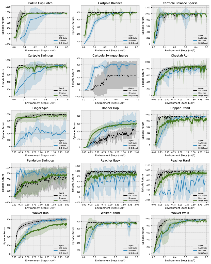
Dreamer Benchmark is a more extensive testbed that was introduced in Dreamer [23], featuring a diverse set of tasks from the DeepMind control suite. Tasks involving sparse reward were excluded (e.g. Acrobot and Quadruped) since they require modification of SAC to incorporate multi-step returns [4], which is beyond the scope of this work. We evaluate on the remaining tasks, fixing the action-repeat hyper-parameter to , as in Dreamer [23].
We compare DrQ [K=2,M=2] to Dreamer [23] and the upper-bound performance of SAC [22] from states222No other publicly reported results are available for the other methods due to the recency of the Dreamer [23] benchmark.. Again, we keep all the hyper-parameters of our algorithm fixed across all the tasks. In Figure 4, DrQ demonstrates the state-of-the-art results by collectively outperforming Dreamer [23], although Dreamer is superior on of the tasks (Walker Run, Cartpole Swingup Sparse and Pendulum Swingup). On many tasks DrQ approaches the upper-bound performance of SAC [22] trained directly on states.
4.2 Atari 100k Experiments
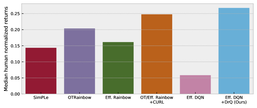
We evaluate DrQ [K=1,M=1] on the recently introduced Atari 100k [31] benchmark – a sample-constrained evaluation for discrete control algorithms. The underlying RL approach to which DrQ is applied is a DQN, combined with double Q-learning [53], n-step returns [42], and dueling critic architecture [56]. As per common practice [31, 54], we evaluate our agent for 125k environment steps at the end of training and average its performance over random seeds. Figure 5 shows the median human-normalized episode returns performance (as in [43]) of the underlying model, which we refer to as Efficient DQN, in pink. When DrQ is added there is a significant increase in performance (cyan), surpassing OTRainbow [32] and Data Efficient Rainbow [54]. DrQ is also superior to CURL [50] that uses an auxiliary loss built on top of a hybrid between OTRainbow and Efficient rainbow. DrQ combined with Efficient DQN thus achieves state-of-the-art performance, despite being significantly simpler than the other approaches. The experimental setup is detailed in Appendix C and full results can be found in Appendix D.
5 Related Work
Computer Vision Data augmentation via image transformations has been used to improve generalization since the inception of convolutional networks [5, 48, 37, 9, 8]. Following AlexNet [35], they have become a standard part of training pipelines. For object classification tasks, the transformations are selected to avoid changing the semantic category, i.e. translations, scales, color shifts, etc. Perturbed versions of input examples are used to expand the training set and no adjustment to the training algorithm is needed. While a similar set of transformations are potentially applicable to control tasks, the RL context does require modifications to be made to the underlying algorithm.
Data augmentation methods have also been used in the context of self-supervised learning. [15] use per-exemplar perturbations in a unsupervised classification framework. More recently, a several approaches [7, 25, 41, 26] have used invariance to imposed image transformations in contrastive learning schemes, producing state-of-the-art results on downstream recognition tasks. By contrast, our scheme addresses control tasks, utilizing different types of invariance.
Regularization in RL Some early attempts to learn RL function approximators used regularization of the Q [18, 58] function. Another approach is entropy regularization [62, 22, 44, 57], where causal entropy is added to the rewards, making the Q-function smoother and facilitating optimization [2]. Prior work has explored regularization of the neural network approximator in deep RL, e.g. using dropout [19] and cutout [11] techniques. See [40] for a comprehensive evaluation of different network regularization methods. In contrast, our approach directly regularizes the Q-function in a data-driven way that incorporates knowledge of task invariances, as opposed to generic priors.
Generalization between Tasks and Domains A range of datasets have been introduced with the explicit aim of improving generalization in RL through deliberate variation of the scene colors/textures/backgrounds/viewpoints. These include Robot Learning in Homes [21], Meta-World [61], the ProcGen benchmark [10]. There are also domain randomization techniques [52, 49] which synthetically apply similar variations, but assume control of the data generation procedure, in contrast to our method. Furthermore, these works address generalization between domains (e.g. synthetic-to-real or different game levels), whereas our work focuses on a single domain and task. In concurrent work, RAD [36] also demonstrates that image augmentation can improve sample efficiency and generalization of RL algorithms. However, RAD represents a specific instantiation of our algorithm when [K=1,M=1] and different image augmentations are used.
Continuous Control from Pixels There are a variety of methods addressing the sample-efficiency of RL algorithms that directly learn from pixels. The most prominent approaches for this can be classified into two groups, model-based and model-free methods. The model-based methods attempt to learn the system dynamics in order to acquire a compact latent representation of high-dimensional observations to later perform policy search [24, 38, 23]. In contrast, the model-free methods either learn the latent representation indirectly by optimizing the RL objective [4, 1] or by employing auxiliary losses that provide additional supervision [60, 50, 47, 16]. Our approach is complementary to these methods and can be combined with them to improve performance.
6 Conclusion
We have introduced a simple regularization technique that significantly improves the performance of SAC trained directly from image pixels on standard continuous control tasks. Our method is easy to implement and adds a negligible computational burden. We compared our method to state-of-the-art approaches on both DeepMind control suite, where we demonstrated that it outperforms them on the majority of tasks, and Atari 100k benchmarks, where it outperforms other methods in the median metric. Furthermore, we demonstrate the method to be robust to the choice of hyper-parameters.
7 Acknowledgements
We would like to thank Danijar Hafner, Alex Lee, and Michael Laskin for sharing performance data for the Dreamer [23] and PlaNet [24], SLAC [38], and CURL [50] baselines respectively. Furthermore, we would like to thank Roberta Raileanu for helping with the architecture experiments. Finally, we would like to thank Ankesh Anand for helping us finding an error in our evaluation script for the Atari 100k benchmark experiments.
References
- [1] Abbas Abdolmaleki, Jost Tobias Springenberg, Yuval Tassa, Remi Munos, Nicolas Heess, and Martin Riedmiller. Maximum a posteriori policy optimisation. arXiv preprint arXiv:1806.06920, 2018.
- [2] Zafarali Ahmed, Nicolas Le Roux, Mohammad Norouzi, and Dale Schuurmans. Understanding the impact of entropy on policy optimization. arXiv preprint arXiv:1811.11214, 2018.
- [3] Jimmy Lei Ba, Jamie Ryan Kiros, and Geoffrey E. Hinton. Layer normalization. arXiv e-prints, 2016.
- [4] Gabriel Barth-Maron, Matthew W. Hoffman, David Budden, Will Dabney, Dan Horgan, Dhruva TB, Alistair Muldal, Nicolas Heess, and Timothy Lillicrap. Distributional policy gradients. In International Conference on Learning Representations, 2018.
- [5] S. Becker and G. E. Hinton. Self-organizing neural network that discovers surfaces in random-dot stereograms. Nature, 1992.
- [6] Richard Bellman. A markovian decision process. Indiana Univ. Math. J., 1957.
- [7] Ting Chen, Simon Kornblith, Mohammad Norouzi, and Geoffrey Hinton. A simple framework for contrastive learning of visual representations. arXiv preprint arXiv:2002.05709, 2020.
- [8] Dan Ciregan, Ueli Meier, and Jurgen Schmidhuber. Multi-column deep neural networks for image classification. In 2012 IEEE conference on computer vision and pattern recognition, pages 3642–3649, 2012.
- [9] Dan C Ciresan, Ueli Meier, Jonathan Masci, Luca M Gambardella, and Jurgen Schmidhuber. High-performance neural networks for visual object classification. arXiv preprint arXiv:1102.0183, 2011.
- [10] Karl Cobbe, Christopher Hesse, Jacob Hilton, and John Schulman. Leveraging procedural generation to benchmark reinforcement learning. arXiv:1912.01588, 2019.
- [11] Karl Cobbe, Oleg Klimov, Chris Hesse, Taehoon Kim, and John Schulman. Quantifying generalization in reinforcement learning. arXiv preprint arXiv:1812.02341, 2018.
- [12] Ronan Collobert, Jason Weston, Leon Bottou, Michael Karlen, Koray Kavukcuoglu, and Pavel Kuksa. Natural language processing (almost) from scratch. Journal of machine learning research, 2011.
- [13] Jacob Devlin, Ming-Wei Chang, Kenton Lee, and Kristina Toutanova. Bert: Pre-training of deep bidirectional transformers for language understanding. arXiv preprint arXiv:1810.04805, 2018.
- [14] Terrance DeVries and Graham W Taylor. Improved regularization of convolutional neural networks with cutout. arXiv preprint arXiv:1708.04552, 2017.
- [15] Alexey Dosovitskiy, Philipp Fischer, Jost Tobias Springenberg, Martin Riedmiller, and Thomas Brox. Discriminative unsupervised feature learning with exemplar convolutional neural networks. TPAMI, 2016.
- [16] Debidatta Dwibedi, Jonathan Tompson, Corey Lynch, and Pierre Sermanet. Learning actionable representations from visual observations. CoRR, 2018.
- [17] Lasse Espeholt, Hubert Soyer, Remi Munos, Karen Simonyan, Volodymir Mnih, Tom Ward, Yotam Doron, Vlad Firoiu, Tim Harley, Iain Dunning, et al. Impala: Scalable distributed deep-rl with importance weighted actor-learner architectures. arXiv preprint arXiv:1802.01561, 2018.
- [18] A. Farahmand, M. Ghavamzadeh, C. Szepesvari, and S. Manor. Regularized policy iteration. In NIPS, 2008.
- [19] Jesse Farebrother, Marlos C. Machado, and Michael Bowling. Generalization and regularization in dqn. arXiv abs/1810.00123, 2018.
- [20] Scott Fujimoto, Herke van Hoof, and David Meger. Addressing function approximation error in actor-critic methods. In Proceedings of the 35th International Conference on Machine Learning, ICML 2018, Stockholmsmassan, Stockholm, Sweden, July 10-15, 2018, 2018.
- [21] Abhinav Gupta, Adithyavairavan Murali, Dhiraj Prakashchand Gandhi, and Lerrel Pinto. Robot learning in homes: Improving generalization and reducing dataset bias. In Advances in Neural Information Processing Systems, 2018.
- [22] Tuomas Haarnoja, Aurick Zhou, Kristian Hartikainen, George Tucker, Sehoon Ha, Jie Tan, Vikash Kumar, Henry Zhu, Abhishek Gupta, Pieter Abbeel, et al. Soft actor-critic algorithms and applications. arXiv preprint arXiv:1812.05905, 2018.
- [23] Danijar Hafner, Timothy Lillicrap, Jimmy Ba, and Mohammad Norouzi. Dream to control: Learning behaviors by latent imagination. arXiv preprint arXiv:1912.01603, 2019.
- [24] Danijar Hafner, Timothy Lillicrap, Ian Fischer, Ruben Villegas, David Ha, Honglak Lee, and James Davidson. Learning latent dynamics for planning from pixels. arXiv preprint arXiv:1811.04551, 2018.
- [25] Kaiming He, Haoqi Fan, Yuxin Wu, Saining Xie, and Ross Girshick. Momentum contrast for unsupervised visual representation learning. arXiv preprint arXiv:1911.05722, 2019.
- [26] Olivier J. Hénaff, Aravind Srinivas, Jeffrey De Fauw, Ali Razavi, Carl Doersch, S. M. Ali Eslami, and Aäron van den Oord. Data-efficient image recognition with contrastive predictive coding. CoRR, 2019.
- [27] Peter Henderson, Riashat Islam, Philip Bachman, Joelle Pineau, Doina Precup, and David Meger. Deep reinforcement learning that matters. Thirty-Second AAAI Conference On Artificial Intelligence (AAAI), 2018.
- [28] Geoffrey E Hinton, Nitish Srivastava, Alex Krizhevsky, Ilya Sutskever, and Ruslan R Salakhutdinov. Improving neural networks by preventing co-adaptation of feature detectors. arXiv preprint arXiv:1207.0580, 2012.
- [29] Max Jaderberg, Volodymyr Mnih, Wojciech Czarnecki, Tom Schaul, Joel Z. Leibo, David Silver, and Koray Kavukcuoglu. Reinforcement learning with unsupervised auxiliary tasks. International Conference on Learning Representations, 2017.
- [30] Leslie Pack Kaelbling, Michael L Littman, and Anthony R Cassandra. Planning and acting in partially observable stochastic domains. Artificial intelligence, 1998.
- [31] Lukasz Kaiser, Mohammad Babaeizadeh, Piotr Milos, Blazej Osinski, Roy H. Campbell, Konrad Czechowski, Dumitru Erhan, Chelsea Finn, Piotr Kozakowski, Sergey Levine, Ryan Sepassi, George Tucker, and Henryk Michalewski. Model-based reinforcement learning for atari. arXiv preprint arXiv:1903.00374, 2019.
- [32] Kacper Piotr Kielak. Do recent advancements in model-based deep reinforcement learning really improve data efficiency? openreview, 2020.
- [33] Diederik P Kingma and Jimmy Ba. Adam: A method for stochastic optimization. arXiv preprint arXiv:1412.6980, 2014.
- [34] Durk P Kingma, Shakir Mohamed, Danilo Jimenez Rezende, and Max Welling. Semi-supervised learning with deep generative models. In Advances in neural information processing systems, pages 3581–3589, 2014.
- [35] Alex Krizhevsky, Ilya Sutskever, and Geoffrey E Hinton. Imagenet classification with deep convolutional neural networks. In Advances in neural information processing systems, 2012.
- [36] Michael Laskin, Kimin Lee, Adam Stooke, Lerrel Pinto, Pieter Abbeel, and Aravind Srinivas. Reinforcement learning with augmented data. arXiv preprint arXiv:2004.14990, 2020.
- [37] Yann LeCun, Bernhard Boser, John S Denker, Donnie Henderson, Richard E Howard, Wayne Hubbard, and Lawrence D Jackel. Backpropagation applied to handwritten zip code recognition. Neural computation, 1989.
- [38] A. X. Lee, A. Nagabandi, P. Abbeel, and S. Levine. Stochastic latent actor-critic: Deep reinforcement learning with a latent variable model. arXiv e-prints, 2019.
- [39] Timothy P. Lillicrap, Jonathan J. Hunt, Alexander Pritzel, Nicolas Heess, Tom Erez, Yuval Tassa, David Silver, and Daan Wierstra. Continuous control with deep reinforcement learning. CoRR, 2015.
- [40] Zhuang Liu, Xuanlin Li, Bingyi Kang, and Trevor Darrell. Regularization matters in policy optimization. arXiv abs/1910.09191, 2019.
- [41] Ishan Misra and Laurens van der Maaten. Self-supervised learning of pretext-invariant representations. arXiv:1912.01991, 2019.
- [42] Volodymyr Mnih, Adria Puigdomenech Badia, Mehdi Mirza, Alex Graves, Timothy P. Lillicrap, Tim Harley, David Silver, and Koray Kavukcuoglu. Asynchronous methods for deep reinforcement learning. CoRR, 2016.
- [43] Volodymyr Mnih, Koray Kavukcuoglu, David Silver, Alex Graves, Ioannis Antonoglou, Daan Wierstra, and Martin Riedmiller. Playing atari with deep reinforcement learning. arXiv e-prints, 2013.
- [44] Ofir Nachum, Mohammad Norouzi, Kelvin Xu, and Dale Schuurmans. Bridging the gap between value and policy based reinforcement learning. In Advances in Neural Information Processing Systems, 2017.
- [45] Edgar Riba, Dmytro Mishkin, Daniel Ponsa, Ethan Rublee, and Gary Bradski. Kornia: an open source differentiable computer vision library for pytorch. In The IEEE Winter Conference on Applications of Computer Vision, pages 3674–3683, 2020.
- [46] Andrew M. Saxe, James L. McClelland, and Surya Ganguli. Exact solutions to the nonlinear dynamics of learning in deep linear neural networks. arXiv e-prints, 2013.
- [47] Pierre Sermanet, Corey Lynch, Yevgen Chebotar, Jasmine Hsu, Eric Jang, Stefan Schaal, Sergey Levine, and Google Brain. Time-contrastive networks: Self-supervised learning from video. In 2018 IEEE International Conference on Robotics and Automation (ICRA), pages 1134–1141. IEEE, 2018.
- [48] Patrice Y Simard, David Steinkraus, John C Platt, et al. Best practices for convolutional neural networks applied to visual document analysis. In Icdar, 2003.
- [49] Reda Bahi Slaoui, William R. Clements, Jakob N. Foerster, and Sébastien Toth. Robust visual domain randomization for reinforcement learning. arXiv abs/1910.10537, 2019.
- [50] Aravind Srinivas, Michael Laskin, and Pieter Abbeel. Curl: Contrastive unsupervised representations for reinforcement learning. arXiv preprint arXiv:2004.04136, 2020.
- [51] Yuval Tassa, Yotam Doron, Alistair Muldal, Tom Erez, Yazhe Li, Diego de Las Casas, David Budden, Abbas Abdolmaleki, Josh Merel, Andrew Lefrancq, et al. Deepmind control suite. arXiv preprint arXiv:1801.00690, 2018.
- [52] Josh Tobin, Rachel Fong, Alex Ray, Jonas Schneider, Wojciech Zaremba, and Pieter Abbeel. Domain randomization for transferring deep neural networks from simulation to the real world. In 2017 IEEE/RSJ international conference on intelligent robots and systems (IROS), 2017.
- [53] Hado van Hasselt, Arthur Guez, and David Silver. Deep reinforcement learning with double q-learning. arXiv e-prints, 2015.
- [54] Hado van Hasselt, Matteo Hessel, and John Aslanides. When to use parametric models in reinforcement learning? arXiv preprint arXiv:1906.05243, 2019.
- [55] Hado P van Hasselt, Matteo Hessel, and John Aslanides. When to use parametric models in reinforcement learning? In Advances in Neural Information Processing Systems, 2019.
- [56] Ziyu Wang, Tom Schaul, Matteo Hessel, Hado Van Hasselt, Marc Lanctot, and Nando De Freitas. Dueling network architectures for deep reinforcement learning. arXiv preprint arXiv:1511.06581, 2015.
- [57] Ronald J Williams and Jing Peng. Function optimization using connectionist reinforcement learning algorithms. Connection Science, 1991.
- [58] Xinyan Yan, Krzysztof Choromanski, Byron Boots, and Vikas Sindhwani. Manifold regularization for kernelized lstd. arXiv abs/1710.05387, 2017.
- [59] Denis Yarats and Ilya Kostrikov. Soft actor-critic (sac) implementation in pytorch. https://github.com/denisyarats/pytorch_sac, 2020.
- [60] Denis Yarats, Amy Zhang, Ilya Kostrikov, Brandon Amos, Joelle Pineau, and Rob Fergus. Improving sample efficiency in model-free reinforcement learning from images. arXiv preprint arXiv:1910.01741, 2019.
- [61] Tianhe Yu, Deirdre Quillen, Zhanpeng He, Ryan Julian, Karol Hausman, Chelsea Finn, and Sergey Levine. Meta-world: A benchmark and evaluation for multi-task and meta reinforcement learning. arXiv preprint arXiv:1910.10897, 2019.
- [62] Brian D. Ziebart, Andrew Maas, J. Andrew Bagnell, and Anind K. Dey. Maximum entropy inverse reinforcement learning. In Proceedings of the 23rd National Conference on Artificial Intelligence - Volume 3, 2008.
Appendix
Appendix A Extended Background
Reinforcement Learning from Images
We formulate image-based control as an infinite-horizon partially observable Markov decision process (POMDP) [6, 30]. An POMDP can be described as the tuple , where is the high-dimensional observation space (image pixels), is the action space, the transition dynamics capture the probability distribution over the next observation given the history of previous observations and current action , is the reward function that maps the current observation and action to a reward , and is a discount factor. Per common practice [43], throughout the paper the POMDP is converted into an MDP [6] by stacking several consecutive image observations into a state . For simplicity we redefine the transition dynamics and the reward function . We then aim to find a policy that maximizes the cumulative discounted return .
Soft Actor-Critic
The Soft Actor-Critic (SAC) [22] learns a state-action value function , a stochastic policy and a temperature to find an optimal policy for an MDP by optimizing a -discounted maximum-entropy objective [62]. is used generically to denote the parameters updated through training in each part of the model. The actor policy is a parametric -Gaussian that given samples , where and and are parametric mean and standard deviation.
The policy evaluation step learns the critic network by optimizing a single-step of the soft Bellman residual
where is a replay buffer of transitions, is an exponential moving average of the weights as done in [39]. SAC uses clipped double-Q learning [53, 20], which we omit from our notation for simplicity but employ in practice.
The policy improvement step then fits the actor policy network by optimizing the objective
Finally, the temperature is learned with the loss
where is the target entropy hyper-parameter that the policy tries to match, which in practice is usually set to .
Deep Q-learning
DQN [43] also learns a convolutional neural net to approximate Q-function over states and actions. The main difference is that DQN operates on discrete actions spaces, thus the policy can be directly inferred from Q-values. The parameters of DQN are updated by optimizing the squared residual error
In practice, the standard version of DQN is frequently combined with a set of tricks that improve performance and training stability, wildly known as Rainbow [53].
Appendix B The DeepMind Control Suite Experiments Setup
B.1 Actor and Critic Networks
We employ clipped double Q-learning [53, 20] for the critic, where each -function is parametrized as a 3-layer MLP with ReLU activations after each layer except of the last. The actor is also a 3-layer MLP with ReLUs that outputs mean and covariance for the diagonal Gaussian that represents the policy. The hidden dimension is set to for both the critic and actor.
B.2 Encoder Network
We employ an encoder architecture from [60]. This encoder consists of four convolutional layers with kernels and channels. The ReLU activation is applied after each conv layer. We use stride to everywhere, except of the first conv layer, which has stride . The output of the convnet is feed into a single fully-connected layer normalized by LayerNorm [3]. Finally, we apply tanh nonlinearity to the dimensional output of the fully-connected layer. We initialize the weight matrix of fully-connected and convolutional layers with the orthogonal initialization [46] and set the bias to be zero.
The actor and critic networks both have separate encoders, although we share the weights of the conv layers between them. Furthermore, only the critic optimizer is allowed to update these weights (e.g. we stop the gradients from the actor before they propagate to the shared conv layers).
B.3 Training and Evaluation Setup
Our agent first collects seed observations using a random policy. The further training observations are collected by sampling actions from the current policy. We perform one training update every time we receive a new observation. In cases where we use action repeat, the number of training observations is only a fraction of the environment steps (e.g. a steps episode at action repeat will only results into training observations). We evaluate our agent every true environment steps by computing the average episode return over evaluation episodes. During evaluation we take the mean policy action instead of sampling.
B.4 PlaNet and Dreamer Benchmarks
We consider two evaluation setups that were introduced in PlaNet [24] and Dreamer [23], both using tasks from the DeepMind control suite [51]. The PlaNet benchmark consists of six tasks of various traits. Importantly, the benchmark proposed to use a different action repeat hyper-parameter for each task, which we summarize in Table 2.
The Dreamer benchmark considers an extended set of tasks, which makes it more difficult that the PlaNet setup. Additionally, this benchmark requires to use the same set hyper-parameters for each task, including action repeat (set to ), which further increases the difficulty.
| Task name | Action repeat |
|---|---|
| Cartpole Swingup | |
| Reacher Easy | |
| Cheetah Run | |
| Finger Spin | |
| Ball In Cup Catch | |
| Walker Walk |
B.5 Pixels Preprocessing
We construct an observational input as an -stack of consecutive frames [43], where each frame is a RGB rendering of size from the th camera. We then divide each pixel by to scale it down to range.
B.6 Other Hyper Parameters
Due to computational constraints for all the continuous control ablation experiments in the main paper and appendix we use a minibatch size of , while for the main results we use minibatch of size . In Table 3 we provide a comprehensive overview of all the other hyper-parameters.
| Parameter | Setting |
| Replay buffer capacity | |
| Seed steps | |
| Ablations minibatch size | |
| Main results minibatch size | |
| Discount | |
| Optimizer | Adam |
| Learning rate | |
| Critic target update frequency | |
| Critic Q-function soft-update rate | |
| Actor update frequency | |
| Actor log stddev bounds | |
| Init temperature |
Appendix C The Atari 100k Experiments Setup
For ease of reproducibility in Table 4 we report the hyper-parameter settings used in the Atari 100k experiments. We largely reuse the hyper-parameters from OTRainbow [32], but adapt them for DQN [43]. Per common practise, we average performance of our agent over random seeds. The evaluation is done for 125k environment steps at the end of training for 100k environment steps.
| Parameter | Setting |
|---|---|
| Data augmentation | Random shifts and Intensity |
| Grey-scaling | True |
| Observation down-sampling | |
| Frames stacked | |
| Action repetitions | |
| Reward clipping | |
| Terminal on loss of life | True |
| Max frames per episode | k |
| Update | Double Q |
| Dueling | True |
| Target network: update period | |
| Discount factor | |
| Minibatch size | |
| Optimizer | Adam |
| Optimizer: learning rate | |
| Optimizer: | |
| Optimizer: | |
| Optimizer: | |
| Max gradient norm | |
| Training steps | k |
| Evaluation steps | k |
| Min replay size for sampling | |
| Memory size | Unbounded |
| Replay period every | step |
| Multi-step return length | |
| Q network: channels | |
| Q network: filter size | , , |
| Q network: stride | |
| Q network: hidden units | |
| Non-linearity | ReLU |
| Exploration | -greedy |
| -decay |
Appendix D Full Atari 100k Results
Besides reporting in Figure 5 median human-normalized episode returns over the Atari games used in [31], we also provide the mean episode return for each individual game in Table 5. Human/Random scores are taken from [54] to be consistent with the established setup.
| Game | Human | Random | SimPLe | OTRainbow | Eff. Rainbow | OT/Eff. Rainbow | Eff. DQN | Eff. DQN |
|---|---|---|---|---|---|---|---|---|
| +CURL | +DrQ (Ours) | |||||||
| Alien | 7127.7 | 227.8 | 616.9 | 824.7 | 739.9 | 1148.2 | 558.1 | 771.2 |
| Amidar | 1719.5 | 5.8 | 88.0 | 82.8 | 188.6 | 232.3 | 63.7 | 102.8 |
| Assault | 742.0 | 222.4 | 527.2 | 351.9 | 431.2 | 543.7 | 589.5 | 452.4 |
| Asterix | 8503.3 | 210.0 | 1128.3 | 628.5 | 470.8 | 524.3 | 341.9 | 603.5 |
| BankHeist | 753.1 | 14.2 | 34.2 | 182.1 | 51.0 | 193.7 | 74.0 | 168.9 |
| BattleZone | 37187.5 | 2360.0 | 5184.4 | 4060.6 | 10124.6 | 11208.0 | 4760.8 | 12954.0 |
| Boxing | 12.1 | 0.1 | 9.1 | 2.5 | 0.2 | 4.8 | -1.8 | 6.0 |
| Breakout | 30.5 | 1.7 | 16.4 | 9.8 | 1.9 | 18.2 | 7.3 | 16.1 |
| ChopperCommand | 7387.8 | 811.0 | 1246.9 | 1033.3 | 861.8 | 1198.0 | 624.4 | 780.3 |
| CrazyClimber | 35829.4 | 10780.5 | 62583.6 | 21327.8 | 16185.3 | 27805.6 | 5430.6 | 20516.5 |
| DemonAttack | 1971.0 | 152.1 | 208.1 | 711.8 | 508.0 | 834.0 | 403.5 | 1113.4 |
| Freeway | 29.6 | 0.0 | 20.3 | 25.0 | 27.9 | 27.9 | 3.7 | 9.8 |
| Frostbite | 4334.7 | 65.2 | 254.7 | 231.6 | 866.8 | 924.0 | 202.9 | 331.1 |
| Gopher | 2412.5 | 257.6 | 771.0 | 778.0 | 349.5 | 801.4 | 320.8 | 636.3 |
| Hero | 30826.4 | 1027.0 | 2656.6 | 6458.8 | 6857.0 | 6235.1 | 2200.1 | 3736.3 |
| Jamesbond | 302.8 | 29.0 | 125.3 | 112.3 | 301.6 | 400.1 | 133.2 | 236.0 |
| Kangaroo | 3035.0 | 52.0 | 323.1 | 605.4 | 779.3 | 345.3 | 448.6 | 940.6 |
| Krull | 2665.5 | 1598.0 | 4539.9 | 3277.9 | 2851.5 | 3833.6 | 2999.0 | 4018.1 |
| KungFuMaster | 22736.3 | 258.5 | 17257.2 | 5722.2 | 14346.1 | 14280.0 | 2020.9 | 9111.0 |
| MsPacman | 6951.6 | 307.3 | 1480.0 | 941.9 | 1204.1 | 1492.8 | 872.0 | 960.5 |
| Pong | 14.6 | -20.7 | 12.8 | 1.3 | -19.3 | 2.1 | -19.4 | -8.5 |
| PrivateEye | 69571.3 | 24.9 | 58.3 | 100.0 | 97.8 | 105.2 | 351.3 | -13.6 |
| Qbert | 13455.0 | 163.9 | 1288.8 | 509.3 | 1152.9 | 1225.6 | 627.5 | 854.4 |
| RoadRunner | 7845.0 | 11.5 | 5640.6 | 2696.7 | 9600.0 | 6786.7 | 1491.9 | 8895.1 |
| Seaquest | 42054.7 | 68.4 | 683.3 | 286.9 | 354.1 | 408.0 | 240.1 | 301.2 |
| UpNDown | 11693.2 | 533.4 | 3350.3 | 2847.6 | 2877.4 | 2735.2 | 2901.7 | 3180.8 |
| Median human-normalised | 1.000 | 0.000 | 0.144 | 0.204 | 0.161 | 0.248 | 0.058 | 0.268 |
| episode returns |
Appendix E Image Augmentations Ablation
Following [7], we evaluate popular image augmentation techniques, namely random shifts, cutouts, vertical and horizontal flips, random rotations and imagewise intensity jittering. Below, we provide a comprehensive overview of each augmentation. Furthermore, we examine effectiveness of these techniques in Figure 6.
Random Shift
We bring our attention to random shifts that are commonly used to regularize neural networks trained on small images [5, 48, 37, 9, 8]. In our implementation of this method images of size are padded each side by pixels (by repeating boundary pixels) and then randomly cropped back to the original size.
Cutout
Horizontal/Vertical Flip
This technique simply flips an image either horizontally or vertically with probability .
Rotate
Here, an image is rotated by degrees, where is uniformly sampled from .
Intensity
Each image tensor is multiplied by a single scalar , which is computed as , where . For our experiments we use and .
Implementation
Finally, we provide Python-like implementation for the aforementioned augmentations powered by Kornia [45].
import torch
import torch.nn as nn
import kornia.augmentation as aug
random_shift = nn.Sequential(nn.ReplicationPad2d(4),aug.RandomCrop((84, 84)))
cutout = aug.RandomErasing(p=0.5)
h_flip = aug.RandomHorizontalFlip(p=0.1)
v_flip = aug.RandomVerticalFlip(p=0.1)
rotate = aug.RandomRotation(degrees=5.0)
intensity = Intensity(scale=0.05)
class Intensity(nn.Module):
def __init__(self, scale):
super().__init__()
self.scale = scale
def forward(self, x):
r = torch.randn((x.size(0), 1, 1, 1), device=x.device)
noise = 1.0 + (self.scale * r.clamp(-2.0, 2.0))
return x * noise
Appendix F K and M Hyper-parameters Ablation
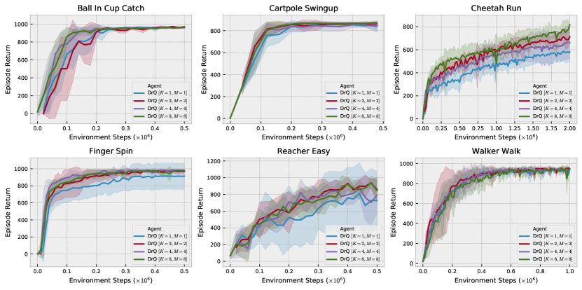
We further ablate the K,M hyper-parameters from Algorithm 1 to understand their effect on performance. In Figure 7 we observe that increase values of K,M improves the agent’s performance. We choose to use the [K=2,M=2] parametrization as it strikes a good balance between performance and computational demands.
Appendix G Robustness Investigation
To demonstrate the robustness of our approach [27], we perform a comprehensive study on the effect different hyper-parameter choices have on performance. A review of prior work [24, 23, 38, 50] shows consistent values for discount and target update rate parameters, but variability on network architectures, mini-batch sizes, learning rates. Since our method is based on SAC [22], we also check whether the initial value of the temperature is important, as it plays a crucial role in the initial phase of exploration. We omit search over network architectures since Figure 1b shows our method to be robust to the exact choice. We thus focus on three hyper-parameters: mini-batch size, learning rate, and initial temperature.
Due to computational demands, experiments are restricted to a subset of tasks from [51]: Walker Walk, Cartpole Swingup, and Finger Spin. These were selected to be diverse, requiring different behaviors including locomotion and goal reaching. A grid search is performed over mini-batch sizes , learning rates , and initial temperatures . We follow the experimental setup from Appendix B, except that only seeds are used due to the computation limitations, but since variance is low the results are representative.
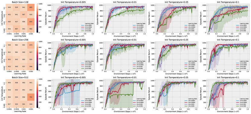
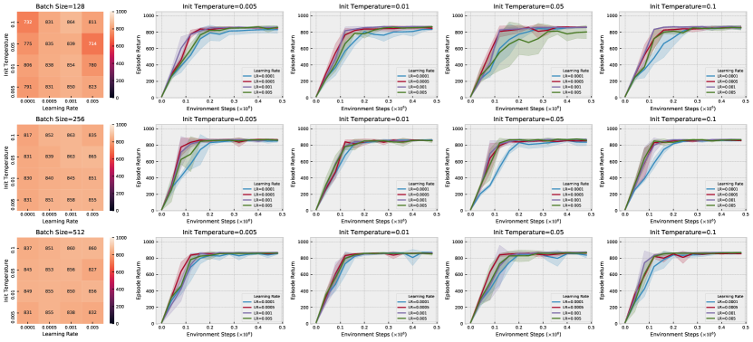
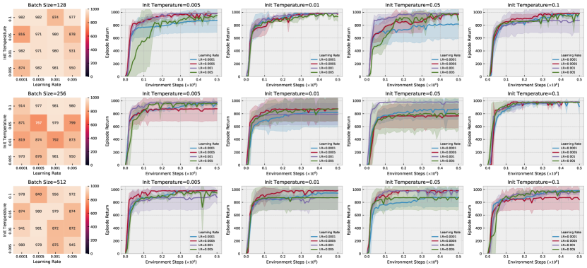
Figure 8 shows performance curves for each configuration as well as a heat map over the mean performance of the final evaluation episodes, similar to [42]. Our method demonstrates good stability and is largely invariant to the studied hyper-parameters. We emphasize that for simplicity the experiments in Section 4 use the default learning rate of Adam [33] (0.001), even though it is not always optimal.
Appendix H Improved Data-Efficient Reinforcement Learning from Pixels
Our method allows to generate many various transformations from a training observation due to the data augmentation strategy. Thus, we further investigate whether performing more training updates per an environment step can lead to even better sample-efficiency. Following [55] we compare a single update with a mini-batch of transitions with updates with different mini-batches of size samples each. Performing more updates per an environment step leads to even worse over-fitting on some tasks without data augmentation (see Figure 9a), while our method DrQ, that takes advantage of data augmentation, demonstrates improved sample-efficiency (see Figure 9b).

