ML-driven Malware that Targets AV Safety

Abstract

Ensuring the safety of autonomous vehicles (AVs) is critical for their mass deployment and public adoption. However, security attacks that violate safety constraints and cause accidents are a significant deterrent to achieving public trust in AVs, and that hinders a vendor’s ability to deploy AVs. Creating a security hazard that results in a severe safety compromise (for example, an accident) is compelling from an attacker’s perspective. In this paper, we introduce an attack model, a method to deploy the attack in the form of smart malware, and an experimental evaluation of its impact on production-grade autonomous driving software. We find that determining the time interval during which to launch the attack is critically important for causing safety hazards (such as collisions) with a high degree of success. For example, the smart malware caused $\mathbf{33\times}$ more forced emergency braking than random attacks did, and accidents in 52.6% of the driving simulations.

I Introduction

Autonomous vehicle (AV) technologies are advertised to be transformative, with the potential to bring greater convenience, improved productivity, and safer roads [1]. Ensuring the safety of AVs is critical for their mass deployment and public adoption [2, 3, 4, 5, 6, 7]. However, security attacks that violate safety constraints and cause accidents are a significant deterrent to achieving public trust in AVs, and also hinder vendors’ ability to deploy AVs. Creating a security hazard that results in a serious safety compromise (for example, an accident) is attractive from an attacker’s perspective. For example, smart malware can modify sensor data at an opportune time to interfere with the inference logic of an AV’s perception module. The intention is to miscalculate the trajectories of other vehicles and pedestrians, leading to unsafe driving decisions and consequences. Such malware can fool an AV into inferring that an in-path vehicle is moving out of the lane while in reality the vehicle is slowing down; that can lead to a serious accident.

This paper introduces i) the foregoing attack model, ii) a method to deploy the attack in the form of smart malware (RoboTack), and iii) an experimental evaluation of its impact on production-grade autonomous driving software. Specifically, the proposed attack model answers the questions of what, how, and when to attack. The key research questions addressed by RoboTack and the main contributions of this paper are:

Deciding what to attack? RoboTack modifies sensor data of the AV such that the trajectories of other vehicles and pedestrians will be miscalculated. RoboTack leverages situation awareness to select a target object for which the trajectory will be altered.

Deciding how to attack? RoboTack minimally modifies the pixels of one of the AV’s camera sensors using an adversarial machine-learning (ML) technique (described in section IV-C) to alter the trajectories of pedestrians and other vehicles, and maintains these altered trajectories for a short time interval. The change in the sensor image and the perceived trajectory is small enough to be considered as noise. Moreover, RoboTack overcomes compensation from other sensors (e.g., LIDAR) and temporal models (e.g., Kalman filters).

Deciding when to attack? RoboTack employs a shallow 3-hidden-layered neural network (NN) decision model (described in section IV-B) to identify the most opportune time with the intent of causing a safety hazard (e.g., collisions) with a high probability of success. In particular, the proposed NN models the non-linear relationship between the AV kinematics (i.e., distance, velocity, acceleration) and attack parameters (i.e., when and how long to attack). We use a feed-forward NN because neural networks can approximate complex continuous functions as shown in the universal function approximation theorem [8].

Assessment on production software. We deployed RoboTack on Apollo [9], a production-grade AV system from Baidu, to quantify the effectiveness of the proposed safety-hijacking attack by simulating ${}^{\sim}2000$ runs of experiments for five representative driving scenarios using the LGSVL simulator [10].

The key findings of this paper are as follows:

1. RoboTack is significantly more successful in creating safety hazards than random attacks (our baseline) are. Here, random attacks correspond to miscalculations of the trajectories (i.e., trajectory hijacking) of randomly chosen non-AV vehicles or pedestrians, at random times, and for random durations. This random attack condition is the most general condition for comparison, although we also show results for a much more restrictive set of experiments. RoboTack caused $\mathbf{33\times}$ more forced emergency braking than random attacks did, i.e., RoboTack caused forced emergency braking in 75.2% of the runs (640 out of 851). In comparison, random attacks caused forced emergency braking in 2.3% (3 out of 131 driving simulations).

2. Random attacks caused 0 accidents, whereas RoboTack caused accidents in 52.6% of the runs (299 out of 568).

3. RoboTack had higher a success rate in attacking pedestrians (84.1% of the runs that involved pedestrians) than in attacking vehicles (31.7% of the runs that involved vehicles).

4. Apollo’s perception system is less robust in detecting pedestrians than in detecting other vehicles. RoboTack automatically discerns that difference, and hence needs only 14 consecutive camera frames involving pedestrians to cause accidents, while needing 48 consecutive camera frames that only involve other vehicles to cause accidents.

Comparing RoboTack with adversarial learning. Past work has targeted deep neural networks (DNNs) used in the perception systems of AVs to create adversarial machine-learning-based attacks [11, 12, 13, 14] that were shown to have successful results (such as by causing misclassification and/or misdetection of a stop sign as a yield sign), and object trackers [15]. The goal of this line of research is to create adversarial objects on the road that fool the AV’s perception system. However, such attacks 1. are limited because DNNs represent only a small portion of the production autonomous driving system (ADS) [9], and 2. have low safety impact due to built-in compensation provided by temporal state-models (which provide redundancy in time) and sensor fusion (which provides redundancy in space) in ADS, which can mask the consequences of such perturbations and preserve AV safety (as shown in this paper, and by others [16]). To summarize, adversarial learning tells one only what to attack. In contrast, as we discuss in detail in section III-D, RoboTack tells one what, when, and how to attack, making it highly efficient in targeting AV safety. Moreover, previous attacks have been shown only on one camera sensor without considering i) the sensor fusion module, and ii) the AV control loop (i.e., it considers only statically captured video frames without running a real ADS). In contrast, we show our attack on an end-to-end production-grade AV system using a simulator that provides data from multiple sensors.

Figure 1: Overview of the ADS perception system and the proposed attack in RoboTack.

II Background

II-A Autonomous Driving Software

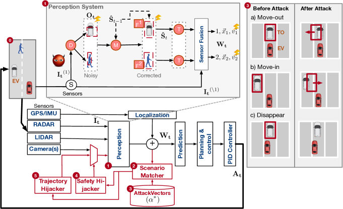
We first discuss the terminologies associated with the autonomous driving system (ADS) that are used in the remainder of the paper. fig. 1 illustrates the basic control architecture of an AV (henceforth also referred to as the Ego vehicle, EV). The EV consists of mechanical components (e.g., throttle, brake, and steering) and actuators (e.g., electric motors) that are controlled by an ADS, which represent the computational (hardware and software) components of the EV. At every instant in time, $t$, the ADS system takes input from sensors $\mathbf{I_{t}}$ (e.g., cameras, LiDAR, GPS, IMU) and infers $\mathbf{W_{t}}$, a model of the world, which consists of the positions and velocities of objects around the EV. Using $\mathbf{W_{t}}$ and the destination as input, the ADS planning, routing, and control module generates actuation commands (e.g., throttle, brake, steering angle). Those commands are smoothed out using a PID controller [17] to generate final actuation values $\mathbf{A_{t}}$ for the mechanical components of the EV. The PID controller ensures that the AV does not make any sudden changes in $\mathbf{A_{t}}$.

II-B Perception System

Definition 1.

Object tracking is defined as the process of identifying an object (e.g., vehicle, pedestrian) and estimating its state $s_{t}$ at time $t$ using a series of sensor measurements (e.g., camera frames, LIDAR pointcloud) observed over time. The state of the object is represented by the coordinates and the size of a “bounding box” (bbox) that contains the object. That estimated state at time $t$ is used to estimate the trajectory (i.e., the velocity, acceleration, and heading) for the object.

Definition 2.

Multiple object tracking (MOT) is defined as the process of estimating the state of the world denoted by $\mathbf{\hat{S}}_{t}=(\hat{s}_{t}^{1},\hat{s}_{t}^{2},...,\hat{s}_{t}^{N_{t}})$, where $N_{t}$ represents the number of objects in the world at time $t$, and $\hat{s}_{t}^{i}$ is the state of the $i$^th object.

The MOT problem is most commonly solved by the tracking-by-detection paradigm [18]. An overview of this paradigm is shown in fig. 1. Here, a sensor (or group of sensors) continuously collects the measurement data at every instant of time $t$ ($\mathbf{I}_{t}$). These sensor inputs are sent to a corresponding DNN-based object detector, such as YoloNet [19] or FasterRCNN [20] (labeled as “D” in fig. 1). Such an object detector estimates the object’s class and its bbox at every time instant. The collection of these bbox measurements for all objects is denoted by $\mathbf{O_{t}}=\{o^{1}_{t},o^{2}_{t},...,o^{M_{t}}_{t}\}$, where $o_{t}^{i}$ denotes the observations for the $i$^th object at time $t$.

An object tracker (or just tracker) tracks the changes in the position of the bboxes over successive sensor measurements. Each detected object is associated with a unique tracker, where a tracker is a Kalman filter [21] (KF) that maintains the state $s^{i}$ for the $i$^th object. Each object detected at time $t$ is associated with either an existing object tracker or a new object tracker, initialized for that object. Such association of a detected object with existing trackers (from time $t-1$) is formulated as a bipartite matching problem, which is solved using the Hungarian matching algorithm [22] (shown as “M” in the figure). “M” uses the overlap, in terms of IoU, between the detected bboxes at time $t$ (i.e., the output of “D”) and the bboxes predicted by the trackers (Kalman filter) of the existing objects to find the matching. A KF is used to maintain the temporal state model of each object (shown as “F^*” in the figure), which operates in a recursive predict-update loop: the predict step estimates the current object state according to a motion model, and the update step takes the detection results ($o^{i}_{t}$) as the measurement to update the $\hat{s}^{i}_{t}$ state. That is, the KF uses a series of noisy measurements observed over time and produces estimates of an object state that tend to be more accurate than those based on a single measurement alone. KF is used to address the following challenges:

• Sensor inputs are captured at discrete times (i.e., $t,\leavevmode\nobreak\ t+1,\dots$). Depending on the speed and acceleration, the object may have moved between those discrete time intervals. Motion models associated with KFs predict the new state of tracked objects from time-step $t-1$ to $t$.

• State-of-the-art object detectors are inherently noisy [19, 20] (i.e., bounding box estimates are approximate measurements of the ground truth), and that can corrupt the object trajectory estimation (i.e., velocity, acceleration, heading). Hence, the perception system uses KFs to compensate for the noise by using Gaussian noise models [22].

Finally, a transformation operation (shown as “T” in the figure) estimates the position, velocity, and acceleration for each detected object by using $\mathbf{\hat{S}_{t}}$. The transformed measurements are then fused with other sensor measurements (e.g., from LiDAR) to get world state $\textbf{W}_{t}$.

Figure 2: Definition of $d_{\text{stop}}$, $d_{\text{safe}}$, and $\delta$ for lateral and longitudinal movement of the car. Non-AV vehicles are labeled as target vehicles (TV).

II-C Safety Model

In this paper, we use the AV safety model provided by Jha et al. [6]. They define the instantaneous safety criteria of an AV in terms of the longitudinal (i.e., direction of the vehicle’s motion) and lateral (i.e., perpendicular to the direction of the vehicle’s motion) Cartesian distance travelled by the AV (see fig. 2). In this paper, we use only the longitudinal definition of the safety model, as our attacks are geared towards driving scenarios for which that is relevant. Below we reproduce the definitions of Jha et al.’s safety model for completeness.

Definition 3.

The stopping distance $d_{\text{stop}}$ is defined as the maximum distance the vehicle will travel before coming to a complete stop, given the maximum comfortable deceleration.

Definition 4.

The safety envelope $d_{\text{safe}}$ [23, 24] of an AV is defined as the maximum distance an AV can travel without colliding with any static or dynamic object.

In our safety model, we compute $d_{\text{safe}}$ whenever an actuation command is sent to the mechanical components of the vehicle. ADSs generally set a minimum value of $d_{\text{safe}}$ (i.e., $d_{\text{safe},\text{min}}$) to ensure that a human passenger is never uncomfortable about approaching obstacles.

Definition 5.

The safety potential $\delta$ is defined as $\delta=d_{\text{safe}}-d_{\text{stop}}$. An AV is defined to be in a safe state when $\delta>0$.

Unlike the authors of [6] who use $\delta\geq 0$ as the safe operation state, we choose $\delta\geq 4$ meters because of a limitation in the simulation environment provided by LGSVL [10] for Apollo [9] that halts simulations for distances closer than $4$ meters.

III Attack Overview & Threat Model

This section describes the attacker goals, target system, and defender capabilities.

III-A Attacker Goals

The ultimate goal of the attacker is to hijack object trajectories as perceived by the AV in order to cause a safety hazard.

To be successful, the attack must:

• Stay stealthy by disguising attacks as noise. To evade detection of his or her malicious intent, an attacker may want to disguise malicious actions as events that occur naturally during driving. In our attack, we hide the data perturbation initiated by the malware/attacker as sensor noise. As we show in section VI-A, modern object detectors naturally misclassify (i.e., identify the object class incorrectly) and misdetect (i.e., bounding boxes have zero or $<60\%$ IoU) objects for multiple time-steps (discussed in section VI-A). Taking advantage of that small error margin in hiding data perturbations, the attacker initiates the attack 1) at the most opportune time such that even if the malicious activity is detected it is too late for the defender to mitigate the attack consequences, and 2) for a short duration of time to evade detection from the intrusion-detection system (IDS) that monitors for spurious activities [25].

• Situational awareness. Hijacking of the object trajectory in itself is not sufficient to cause safety violations or hazardous driving situations. An attacker must be aware of the surrounding environment to initiate the attack at the most opportune time to cause safety hazards (e.g., collisions).

• Attack automation. An attacker can automate the process of monitoring and identifying the opportune time for an attack. That way, the adversary only needs to install the malware instead of manually executing the attack.

III-B Threat Model

In this section, we discuss the target system, the existing defenses, and the attacker’s capabilities.

Target system. The target is the perception system of an AV, specifically the object detection, tracking, and sensor fusion modules. To compensate for the noise in the outputs of the object detectors, the AV perception system uses temporal tracking and sensor fusion (i.e., fusion data from multiple sensors such as LIDAR, RADAR, and cameras). Temporal tracking and sensor fusion provide an inherent defense against most if not all existing adversarial attacks on detectors [16].

The critical vulnerable component of the perception system is a Kalman filter (KF) (see “F” in section II and fig. 1). KFs generally assume that measurement noise follows a zero-mean Gaussian distribution, which is the case for the locations and sizes of bboxes produced by the object detectors (described later in section VI-A). However, that assumption introduces a vulnerability. The KF becomes ineffective in compensating for the adversarially added noise. We show in this paper that an attacker can alter the trajectory of a perceived object by adding noise within one standard deviation of the modeled Gaussian noise.

The challenge in attacking a KF is to maintain a small attack window (i.e., the number of contiguous time epochs for which the data are perturbed). When an attacker is injecting a malicious noise pattern, the attack window must be sufficiently small (1–60 time-steps) such that the defender cannot estimate the distribution of the injected noise and hence cannot defend the system against the attack.

What can attackers do? In this paper we intentionally and explicitly skirt the problem of defining the threat model. Instead, we focus on what an attacker could do to an AV if he or she has access to the ADS source code and live camera feeds.

Gain knowledge of internal ADS system. We assume that the attacker has obtained knowledge of the internal ADS system by analyzing the architecture and source code of open-source ADSs, e.g., Apollo [9, 26]. The attacker can also gain access to the source code through a rogue employee.

Gain access to and modify live camera feed. Recently, Argus [27] showed the steps to hijack a standalone automotive-grade Ethernet camera and spoof the camera traffic. The attack follows a “man-in-the-middle” (MITM) strategy in which an adversary gains physical access to the camera sensor data and modifies them (when certain conditions are met). The hack relied on the fact that the camera traffic is transmitted using standard (i.e., IEEE 802.1 Audio Video Bridging [28]) but simple protocols, which do not use encryption because of the size of the data as well as performance and latency constraints associated with the transmission. As the camera feed is not encrypted, the attacker can reassemble packages of a video frame and decode the JFIF (JPEG File Interchange Format) payload into an image. Most importantly, since there is no hash or digital signature checks on the transmitted images, to prepare for the attack, the attacker can apply a number of filters to modify the images in-line without being noticed. The MITM attack works by using an Ethernet tap device to capture UDP packets in the Ethernet/RCA link between the camera and the ADS software. The Ethernet tap captures images and provides them as the input for attacker-controlled hardware with purpose-built accelerators, such as NVIDIA EGX, that are operating outside the domain of the ADS hardware/software.

Optionally, compromise ADS software using secret hardware implant. To further hide malware and evade detection, an attacker can install backdoors in the hardware. Injection of malicious code in hardware-software stacks has been realized in existing hardware backdoors embedded in CPUs, networking routers, and other consumer devices [29, 26]. As an AV is assembled from components supplied by hundreds of vendors through a sophisticated supply chain, it is reasonable to argue that individual components such as infotainment systems and other existing electronic component units (ECUs) could be modified to enable secret backdoors [30, 26].

What things can attackers not do? In this work, we assume that the CAN bus transmitting the control command is protected/encrypted. Therefore we cannot launch a man-in-the-middle attack to perturb the control/actuation commands sent to the mechanical components of the EV.

Defender capabilities. Again, we assume that the CAN bus transmitting the controller/actuation commands is encrypted. That assumption is acceptable because many commercial products utilize such encryption[31]. Moreover, there are well known IDSs for monitoring CAN bus activity [25, 32]. Therefore, we do not leverage CAN bus vulnerabilities as an attack vector; instead, our attack exploits vulnerabilities on the camera’s Ethernet/RCA cable link.

III-C Attack Vectors and Injected Attacks

We describe a taxonomy of attack vectors (shown in fig. 1) that the attacker can leverage to maximize impact, such as with an emergency stop or a collision. The attack vectors are as follows.

• Move_Out. In this attack, the attacker hijacks the target object (TO) trajectories to fool the EV into believing that the TO is moving out of the EV’s lane. A close variant of this attack is fooling the EV into believing that the target object is maintaining its lane, whereas in reality the target object is moving into the EV’s lane. Because of this attack, the EV will start to accelerate or maintain its speed, causing it to collide with the target object.

• Move_In. In this attack, the attacker hijacks the target object (TO) trajectories to fool the EV into believing that the TO is moving into the EV’s lane. Because of this attack, the EV will initiate emergency braking. The emergency braking maneuver is highly uncomfortable for the passengers of the EV and may lead to injuries in some cases.

• Disappear. In this attack, the attacker hijacks the target object (TO) trajectories to fool the EV into believing that the TO has disappeared. The effects of this attack will be similar to those of the Move_Out attack model.

Figure 3: Steps followed by RoboTack to mount a successful attack, i.e., collision between the EV (blue) and the target object (red). SM: Scenario matching. SH: Safety hijacking, TH: Trajectory hijacking.

III-D Attack Phases.

The attack progresses in three key phases as follows.

Phase 1. Preparing and deploying the malware. Here the attacker does the following:

1. Gains access to the ADS source code,

2. Defines the mapping between the attack vectors (see section III-C) and the world state ($\mathbf{W}_{t}$),

3. Trains the "safety hijacker" and fine-tunes the weights of "trajectory hijacker" (e.g., learns about the maximum perturbation that can be injected to evade detection) for the given ADS,

4. Gains access to the target EV camera feeds, and

5. Installs RoboTack on the target EV.

Phase 2. Monitoring the environment. Once our intelligent malware is deployed, it does the following:

1. Approximately reconstructs the world ($\mathbf{{W}}_{t}$) using the hacked camera sensor data ( in fig. 1). For simplicity, we assume that the world state estimated using sensor fusion is not significantly different from the state determined using only one camera sensor. In our implementation, we only use $\mathbf{\hat{S}}_{t}$ to carry out the attack instead of relying on data from all sensors.

2. Identifies the victim target object $i$ (i.e., one of the other vehicles or pedestrians) for which the trajectory is hijacked. The target object is the one closest to the EV. The identification is done using the safety model as defined in section II-C (line 9 of algorithm 1).

3. Invokes the “scenario matcher” (SM) module ( in fig. 1), which uses the world state ($\mathbf{W}_{t}$) to determine whether the identified object is vulnerable to one of the attack vectors (as shown in and discussed in section III-C).

4. Uses the “safety hijacker” (SH) (shown as in fig. 1) to decide when to launch the attack ($t$), and for how long ($t+K$). The SH estimates the impact of the attack by using a shallow 3-hidden-layered NN, in terms of reduced safety potential ($\delta$). The malware launches the attack only if the reduced safety potential drops below a predefined threshold (10 meters). We determine the threshold through simulation of driving scenarios that lead to emergency braking by the EV. To evade detection, the malware ensures that $K$ does not exceed a pre-defined threshold (see line 15 in algorithm 1). $K$ is obtained by characterizing the continuous misdetection of an object associated with the “object detector” in the normal (i.e., without attacks) driving scenarios executed in the simulator.

Phase 3. Triggering the attack. RoboTack:

1. Uses the “trajectory hijacker” ( in fig. 1) to corrupt the camera feed. The trajectory hijacker perturbs the camera sensor data such that i) the trajectory of the object (e.g., a school bus) is altered to match the selected attack vector (e.g., Move_Out), and ii) the trajectory of the object does not change significantly, thus evading detection.

2. Attacks the trajectory of the victim object for the next $K$ time-steps, chosen by the safety hijacker.

III-E An Example of a Real Attack

fig. 3 shows an example of a Move_Out attack. Here we show two different views: i) a simulation view, which was generated using a driving scenario simulator, and ii) an ADS view, which was rendered using the world-state visualizer.

RoboTack continuously monitors every camera frame using “scenario matching” (SM) to identify a target object for which the perceived trajectory by the EV can be hijacked. If SM does not identify any target object of interest, it skips the rest of the step and waits for the next camera frame. As shown in fig. 3 (a) and (b), at time-step $t$, SM identified an SUV (i.e., target vehicle) as a target object of interest, and returned "Move_Out" as a matched attack vector, as the SUV was already in the Ego lane. Next, RoboTack launched "safety hijacker" to determine the reduced safety potential of the attack and the number of time-steps the attack would need to be maintained. As it turns out, the "safety hijacker" determined that the reduced safety potential could cause an accident, so RoboTack launched "trajectory hijacker" to perturb the camera sensor data as shown in fig. 3 (c). Its impact on the trajectory is shown in fig. 3(d). Camera sensor data are perturbed by modifying individual pixels as shown in the white area (in the bounding box (red square) of the target object) for illustration purposes, because originally these pixels were modified in a way that was almost invisible to the human eye. Because of this attack, the EV collided with the target object as shown in fig. 3(e) and (f).

1:$\mathbf{\hat{S}_{t-1:t-2}}$ $\triangleright$ Past object states

2:$\mathbf{I_{t}^{1}}$ $\triangleright$ Camera feed

3:$attack$ $\triangleright$ Flag indicating if the attack is active

4:$K$ $\triangleright$ Number of continuous attacks

5:$i$ $\triangleright$ Index of the target object

6:$\mathbf{I_{t}^{1}}^{\prime}$ $\triangleright$ Perturbed image with adversarial patch

7:$\alpha\leftarrow\varnothing$

8:$\mathbf{O_{t}},\mathbf{\hat{S}_{t}}\leftarrow Perception(I_{t})$

9:if $attack=False$ then

10:     $i,\delta_{t}\leftarrow SafetyModel(\mathbf{\hat{S}_{t}})$ $\triangleright$ From definition 5

11:     $\vec{v}_{rel,t}^{i}\leftarrow calcVelocity({\hat{s}}_{t:t-1}^{i})$

12:     $\vec{a}_{rel,t}^{i}\leftarrow calcAcceleration({\hat{s}}_{t:t-2}^{i})$

13:     $\alpha\leftarrow ScenarioMatcher({\hat{s}_{t}^{i}})$

14:end if

15:if $\alpha\neq\varnothing$ then

16:     $attack,K\leftarrow SafetyHijacker(\vec{a}_{rel,t}^{i},\vec{v}_{rel,t}^{i},\vec{\delta}_{t},\alpha$)

17:end if

18:if $attack=True\leavevmode\nobreak\ \land\leavevmode\nobreak\ K>0$  then

19:     $\mathbf{I_{t}^{1}}^{\prime}\leftarrow TrajectoryHijacker(i,\mathbf{I_{t}^{1}},{o_{t}^{i}},{\hat{s}_{t-1}^{i}},\alpha)$

20:     $K\leftarrow K-1$

21:     if $K=0$ then

22:         $attack\leftarrow False$

23:     end if

24:end if

Algorithm 1 Attack procedure at each time-step.

IV Algorithms and Methodology

In this section, we outline the three key steps taken by the malware: 1. in the monitoring phase, selecting the candidate attack vector by using the scenario matcher (section IV-A); 2. in the monitoring phase, deciding when to attack by using the safety hijacker (section IV-B); and 3. in the trigger phase, perturbing camera sensor feeds using the trajectory hijacker. These steps are described in algorithm 1.

IV-A Scenario Matcher: Selecting the Target Trajectory

The goal of the scenario matcher is to check whether the closest object to the EV (referred to as the target object) is vulnerable to any of the candidate attack vectors (i.e., Move_Out, Move_In, and Disappear). This is a critical step for the malware, as it wants to avoid launching 1) an attack if there are no objects next to or in front of the EV; or 2) an attack when the object is actually executing the would-be bogus driving maneuver (e.g., selecting attack vector $\alpha$ = Move_Out when the target is moving out of the Ego lane anyway). The scenario-matching algorithm is intentionally designed as a rule-based system (whose rules are listed in table I) to minimize its execution time, and hence evade detection.

Note that "Scenario Matcher" can interchangeably choose between the Move_Out and Disappear attack vectors. However, in our work, we found that Disappear, which requires a large perturbation in trajectory, is better suited for attacking the pedestrians because the attack window is small. In contrast, the attack window for vehicles is large. Therefore, for vehicles, RoboTack uses Move_Out. This is described in detail in section VI.

IV-B Safety Hijacker: Deciding When to Attack

To cause a safety violation (i.e., a crash or emergency brake), the malware will optimally attack the vehicle when the attack results in $\delta\leavevmode\nobreak\ \leq\leavevmode\nobreak\ 4$ meters. The malware incorporates that insight into the safety hijacker to choose the start and stop times of the attack by executing the safety hijacker at every time-step. The safety hijacker at time-step $t$ takes ($\vec{v}_{rel,t}^{i},\vec{a}_{rel,t}^{i}$), $\delta_{t}$, and $\alpha$ as inputs. It outputs the attack decision (i.e., attack or no-attack) and the number of time-steps $K$ for which the attack must continue to be successful (line 16 in algorithm 1).

TO trajectory	TO in EV-lane	TO not in EV-lane
Moving In	—	Move_Out/Disappear
Keep	Move_Out/Disappear	Move_In
Moving Out	Move_In	—

• TO: Target object

Table I: Scenario Matching Map

Let us assume that the malware has access to an oracle function $f_{\alpha}$ for a given attack vector $\alpha$ that predicts the future safety potential of the EV when it is subjected to the attack type $\alpha$ for $k$ continuous time-steps,

$$\delta_{t+k}=\mathit{f_{\alpha}}(\vec{v}_{rel,t}^{i},\vec{a}_{rel,t}^{i},\delta_{t},k).$$ (1)

Later in this section, we will describe a machine-learning formulation that approximates $f_{\alpha}$ using a neural network, and describe how to integrate it with the malware. The malware decides to attack only when the safety potential $\delta_{t+k}$ is less than some threshold $\gamma$. Ideally, the malware should attack when $\gamma=4$ (i.e., corresponding to the the $\delta$ for the crash).

In order to evade detection and disguise the attack as noise, the installed malware should choose the "optimal $k$," which we refer to as $K$ (i.e., the minimal number of consecutive camera sensor frame perturbations), using the information available at time-step $t$. The malware can use the oracle function $f_{\alpha}(.)$ to decide on the optimal number of time-steps ($K$) for which the attack should be active. The malware decides to attack only if $k\leq K_{max}$, where $K_{max}$ is the maximal number of time-steps during which a corruption of measurements cannot be detected. This is formalized in eq. 2.

$$K=\underset{k}{argmin}\leavevmode\nobreak\ k\cdot\left(\mathbb{I}(\delta_{t+k}\leq\gamma)=1\right)$$ (2)

Finally, the malware must take minimal time to arrive at the attack decision. However, in the current formulation, calculating $K$ can be very costly, as it is necessary to evaluate eq. 2 using $f_{\alpha}$ (which is an NN) for all $k\leq K_{max}$. We accelerate the evaluation of $K$ by leveraging the fact that for our scenarios (section V-C), $f_{\alpha}$ is non-increasing with increasing $k$ when $\vec{a}_{{rel}_{t}}\leq 0$. Hence, we can do a binary search between $k\in[0,K_{max}]$ to find $K$ in $O(\log{}K_{max})$ steps.

Estimating $\mathit{f_{\alpha}}$ using an NN. We approximate the oracle function $f_{\alpha}$ using a feed-forward NN. We use an NN to approximate $f_{\alpha}$ to model the uncertainty in the ADS due to use of non-deterministic algorithms. Hence, the malware uses a uniquely trained NN for each attack vector. The input to the NN is a vector $[\delta_{t},\vec{v}_{rel_{t}},\vec{a}_{rel_{t}},k]$. The model predicts $\delta_{t+k}$ after $k$ consecutive frames, given the input. Intuitively, the NN learns the behavior of the ADS (e.g., conditions for emergency braking) and kinematics under the chosen attack vector, and it infers the safety potential ${\delta}_{t+k}$ to the targeted object from the input. We train the NN using a cost function ($\mathcal{L}$) that minimizes the average $L2$ distance between the predicted ${\delta}_{{t+k}}$ and the ground-truth ${\delta^{G}_{{t+k}}}$ for the training dataset $\mathcal{{D}}_{train}$.

$$\mathcal{L}=\frac{1}{|\mathcal{{D}}_{train}|}\sum_{i\in\mathcal{{D}}_{train}}\|{\delta^{G,i}_{t+k}}-{\delta}^{i}_{{t+k}}\|^{2}_{2}$$ (3)

We use a fully connected NN with 3 hidden layers ($100,100,50$ neurons), the ReLU activation function, and dropout layers with a dropout rate of $0.1$ to estimate $\mathit{f_{\alpha}}$. The specific architecture of the NN was chosen to reduce the computational time for the inference with sufficient learning capacity for high accuracy. The NN predicts the safety potential after the attack within 1m and 5m for pedestrian and vehicles, respectively.

The NN was trained with a dataset $\mathcal{{D}}$ collected from a set of driving simulations ran on Baidu’s Apollo ADS. To collect training data, we ran several simulations, where each simulation had a predefined $\delta_{inject}$ and a $k$, i.e., an attack started as soon as the $\delta_{t}=\delta_{inject}$, and continued for $k$ consecutive time-steps. The dataset characterized the ADS’s responses to attacks. The network was trained using the Adam optimizer with a 60%-40% split of the dataset between the training and the validation.

IV-C Hijacking Trajectory: Perturbing Camera Sensor Feeds

In this section, we describe the mechanism through which the malware can perturb the camera sensor feeds to successfully mount the attack (i.e., execute one of the attack vectors) once it has decided to attack the EV. The malware achieves that objective using a trajectory hijacker.

The attack vectors used in this paper require that the malware perturb the camera sensor data (by changing pixels) in such a way that the bounding box (${\hat{s}_{t}^{i}}$) estimated by the multiple-object tracker (used in the perception module) at time $t$ moves in a given direction (left or right) by $\omega_{t}$.

The objective of moving the bounding box ${\hat{s}_{t}^{i}}$ in a given direction (left or right) can be formulated as an optimization problem. To solve it, we modify the model provided by Jia et al.[15] to evade attack detection. We find the translation vector $\omega_{t}$ at time $t$ that maximizes the cost $\mathbf{M}$ of Hungarian matching (recall $\mathbf{M}$ from fig. 1) between the detected bounding box, ${o_{t}^{i}}$, and the existing tracker state $\hat{s}_{t-1}^{i}$ (i.e., pushing the ${o_{t}^{i}}$ away from $\hat{s}_{t-1}^{i}$) such that the following conditions hold:

• Threshold $\mathbf{M}\leq\lambda$ ensures that ${o_{t}^{i}}$ must still be associated with its original tracker state ${\hat{s}_{t-1}^{i}}$, i.e., $\mathbf{M}\leq\lambda$. $\lambda$ can be found experimentally for a given perception system and depends on Kalman parameters. This condition is relaxed when the selected attack $\alpha=\text{"Disappear."}$

• $\omega_{t}\in[\mu-\sigma,\mu+\sigma]$ is within the Kalman noise parameters ($\mu,\sigma$) of the selected candidate object. This condition ensures that the perturbation is within the noise.

• Threshold $IoU({o}_{t}^{i}+\omega_{t},\leavevmode\nobreak\ patch)\geq\gamma$ ensures that the adversarial patch $patch$ should intersect with the detected bounding box, ${o_{t}^{i}}$, to restrict the search space of the patch. This condition can be removed when the attacker has access to the ADS, and can directly perturb $o_{t}^{i}$.

$$\underset{\omega_{t}}{max}\leavevmode\nobreak\ \mathbf{M}\leavevmode\nobreak\ ({o_{t}^{i}}+\omega_{t}, \leavevmode\nobreak\ {\hat{s}_{t-1}^{i}})$$ (4)

$$\textit{s.t.}\leavevmode\nobreak\ \mathbf{M} \leq\lambda,$$

$$\leavevmode\nobreak\ IoU({o}_{t}^{i}+\omega_{t},\leavevmode\nobreak\ patch) \geq\gamma,$$

$$\omega_{t} \in[\mu-\sigma,\mu+\sigma]$$

Finally, the malware should stop maximizing the distance between the ${o_{t}^{i}}$ and ${\hat{s}_{t-1}^{i}}$ when the object tracker has moved laterally by $\Omega$ (i.e., the difference between the observed lateral distance and the estimated lateral distance) since the attack start time $t-K^{\prime}$.

In our experiments, we found $K^{\prime}$ to be generally around 4–20 frames, whereas $K$ (i.e., total attack time determined by safety hijacker) was found to be generally 10–65 frames. Since $K^{\prime}$ is small, the chances of detection are significantly lower.

Perturbing Camera Sensor Data. Here the goal of the perturbation is to shift the position of the object detected by the object detector (e.g., YOLOv3). To achieve that objective, we formulate the problem of generating perturbed camera sensor data using Eq. (2) in [15]. We omit the details because of lack of space.

IV-D Implementation

We implemented RoboTack using Python and C++. Moreover, we used fault injection-based methods to implement the attack steps of RoboTack. The proposed malware has a small footprint, i.e., less than 500 lines of Python/C++ code, and 4% additional GPU utilization with negligible CPU utilization in comparison to the autonomous driving stack. This makes it difficult to detect an attack using methods that monitor the usage of system resources.

V Experimental Setup

V-A AI Platform

In this work, we use Apollo [9] as an AI agent for driving the AV. Apollo is built by Baidu and is openly available on GitHub [33]. However, we use LGSVL’s version of Apollo 5.0 [34], as it provides features to support integration of the LGSVL simulator [10] with Apollo. Apollo uses multiple sensors: a Global Positioning System (GPS), Inertial measurement units (IMU), radar, LiDAR, and multiple cameras. Our setup used two cameras (fitted at the top and front of the vehicle) and one LiDAR for perception.

V-B Simulation Platform

We used the LGSVL simulator [10] that uses Unity [35], a gaming engine  [36], to simulate driving scenarios. Note that a driving scenario is characterized by the number of actors (i.e., objects) in the world, their initial trajectories (i.e., position, velocity, acceleration, and heading), and their waypoints (i.e., their route from source to destination). In our setup, LGSVL simulated the virtual environment and posted virtual sensor data to the ADS for consumption. The sensors included a LiDAR, a front-mounted main camera, a top-mounted telescope camera, IMU, and GPS. The measurements for different sensors were posted at different frequencies [37]. In our experiments, the cameras produced data at 15 Hz (of size 1920x1080), GPS at 12.5 Hz, and LiDAR is rotating at 10 Hz and producing $360^{\circ}$ measurements per rotation. At the time of this writing, LGSVL does not provide integration of continental radar for Apollo. In addition, LGSVL provides Python APIs for creating driving scenarios, which we leveraged to develop the driving scenarios described next.

V-C Driving Scenarios

Here we describe the driving scenarios, shown in fig. 4, that were used in our experiments. All our driving scenarios were generated using LGSVL on "Borregeas Avenue" (located in Sunnyvale, California, USA), which has a speed limit of 50 kph. Unless otherwise specified, in all the cases EV was cruising at 45 kph.

Figure 4: Driving scenarios. EV: Ego Vehicle. TV: Target Vehicle. NPC: Other Vehicles with no interaction with EV.

In driving scenario 1 or "DS-1," the Ego vehicle (EV) followed a target vehicle (TV) in the Ego lane at a constant speed (25 kph), as shown in Figure 4. The TV started 60 meters ahead of the EV. In the golden (i.e., non-attacked) run, the EV would accelerate to 40 kph and come closer to the TV at the beginning, and then gradually decelerate to 25 kph to match the speed of the TV. Thereafter, the EV maintained a longitudinal distance of 20 meters behind the TV for the rest of the scenario. We used this scenario to evaluate the Disappear and Move_Out attack vectors on a vehicle.

In driving scenario 2 or "DS-2," a pedestrian illegally crossed the street as shown in Figure 4. In the golden run, the EV braked to avoid collision and stopped more than 10 meters away from the pedestrian, if possible. The EV started traveling again when the pedestrian moved off the road. We used this scenario to evaluate the Disappear and Move_Out attack vectors on a pedestrian.

In driving scenario 3 or "DS-3," a target vehicle was parked on the side of the street in the parking lane. In the golden run, the EV maintained its trajectory (lane keeping). We used this scenario to evaluate the Move_In attack vector on a vehicle.

In driving scenario 4 or "DS-4," a pedestrian walked longitudinally towards the EV in the parking lane (next to the EV lane) for 5 meters then stood still for the rest of the scenario. In the golden run, EV recognized the pedestrian, at which point it reduced its speed to 35 kph. However, once it ensured that the pedestrian was safe (by evaluating its trajectory), it resumed its original speed. We use this scenario to evaluate the Move_In attack vector on a pedestrian.

In driving scenario 5 or "DS-5," there are multiple vehicles with random waypoints and trajectories, as shown in Figure 4. Throughout the scenario, the EV was set to follow a target vehicle just as in "DS-1," with multiple non-AV vehicles traveling on the other lane of the road as well as in front or behind (not shown). Apart from the target vehicle, the vehicles traveled at random speeds and starting from random positions in their lanes. We used this scenario as the baseline scenario for a random attack to evaluate the effectiveness of our attack end-to-end.

V-D Hardware Platform

The production version of the Apollo ADS is supported on the Nuvo-6108GC [38], which consists of Intel Xeon CPUs and NVIDIA GPUs. In this work, we deployed Apollo on an x86 workstation with a Xeon CPU, ECC memory, and two NVIDIA Titan Xp GPUs.

VI Evaluation & Discussion

VI-A Characterizing Perception System on Pretrained YOLOv3 in Simulation

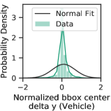
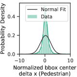
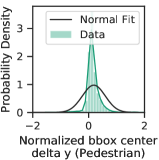
We characterize the performance of YOLOv3 (used in the Apollo perception system) in detecting objects on the road, while the AV is driving, to measure 1. the distribution of successive frames from an AV camera feed in which a vehicle or a pedestrian is continuously undetected, and 2. the distribution of error in the center positions of the predicted bounding boxes compared to the ground-truth bounding boxes. We characterize those quantities to show that an attack mounted by RoboTack and the natural noise associated with the detector are from the same distribution. In particular, we show that the continuous misdetection caused by RoboTack is within the 99th percentile of the continuous characterized misdetection distribution of the YOLOv3 detector; see Figure 5. That is important because if our attack fails, the object will reappear and be flagged by the IDS as an attack attempt. Similarly, we characterize the error in the predicted bounding box to ensure that our injected noise is within the estimated Gaussian distribution parameters shown in Figure 5. RoboTack changes the position at time-step $t$ by at max $\mu-\sigma\leq\omega\leq\mu+\sigma$ of the Gaussian distribution. For this characterization, we generated a sequence of images and labels (consisting of object bounding boxes and their classes) by manually driving the vehicle on the San Francisco map for 10 minutes in simulation.

Continuous misdetections. fig. 5 (a) and (b) show the distribution of the number of frames in which pedestrians and vehicles were continuously misdetected. Here we consider an object as misdetected if the IoU between the predicted and ground-truth bounding boxes is less than $60\%$. The data follow an exponential distribution.

(a) Exp(loc = 1, $\lambda$ = 0.717)
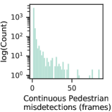
99th perc: 31.0

(b) Exp(loc = 1, $\lambda$ = 0.327)
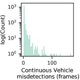
99th perc: 59.4

(c) Normal($\mu$ = 0.023, $\sigma$ = 0.464)
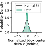
99th perc: 1.145

(d) Normal($\mu$ = 0.094, $\sigma$ = 0.586)
99th perc: 1.775

(e) Normal($\mu$ = 0.254, $\sigma$ = 2.010)
99th perc: 5.235

(f) Normal($\mu$ = 0.186, $\sigma$ = 0.409)
99th perc: 1.868

Figure 5: YOLOv3 object detection characterization on driving video generated using LGSVL. (a–b) show continuous misdetections with IoU=60%. (c–f) show the distribution of normalized errors in the bounding box center predictions along the x and y coordinates of the image for vehicles and pedestrians.

Bounding box prediction error. To characterize the noise in the position of the bounding boxes predicted by YOLOv3, we computed the difference between the center of the predicted bounding box and the ground-truth bounding box and normalized it by the size of the ground-truth bounding box.

Only predicted bounding boxes that overlap with the ground-truth boxes are considered. fig. 5(c), (d), (e), and (f) show the distribution of normalized errors for the x (horizontal) and y (vertical) coordinates in the image of the bounding box centers for pedestrians and vehicles. The coordinates of the centers of the YOLOv3-predicted bounding boxes follow a Gaussian noise model.

ID	$K$	# runs	# EB (%)	# crashes (%)
DS-1-Disappear-R	48	101	54 (53.5%)	32 (31.7%)
DS-2-Disappear-R	14	144	136 (94.4%)	119 (82.6%)
DS-1-Move_Out-R	65	185	69 (37.3%)	32 (17.3%)
DS-2-Move_Out-R	32	138	135 (97.8%)	116 (84.1%)
DS-3-Move_In-R	48	148	140 (94.6%)	—
DS-4-Move_In-R	24	135	106 (78.5%)	—
DS-5-Baseline-Random	K*	131	3 (2.3%)	0

Table II: Smart malware attack summary compared with random (in bold). EB: Emergency Braking. R: Robotack. In our experiments, the AV tried emergency braking in all runs that resulted in accidents. K* means K was randomly picked between 15 and 85 for each run of the experiment.

VI-B Quantifying Baseline Attack Success

In the baseline attack (Baseline-Random), we altered the object trajectory by (i) randomly choosing an object (i.e., a vehicle or a pedestrian) for which the trajectory will be changed, (ii) randomly choosing the attack vector for a simulation run, (iii) randomly initiating the attack at time-step $t$ of the driving scenario, and (iv) continuing the attack for (a randomly chosen) $K$ time-steps. In other words, Baseline-Random) attack neither used scenario matcher nor used safety hijacker to mount the attack on the AV. However, it mimics trajectory hijacker to modify the trajectory of the vehicle. We used 131 experimental runs of DS-5 in which the AV was randomly driving around the city to characterize the success of the baseline attack. Across all 131 experimental runs (see "DS-5-Baseline-Random," table II), the AV performed emergency braking (EB) in only 3 runs (2.3%) and crashed 0 times.

Here we also compare RoboTack with attacks where both scenario matcher and trajectory hijacker are used (labeled as "R w/o SH" in fig. 6). However, these attacks do not use safety hijacker (SH). Hence, in these attacks, we randomly initiated the attack, and continue to attack for (a randomly chosen) $K$ time-steps, where $K$ is between 15 and 85. The results of these attacks are described in detail in section VI-D.

Taken together these experiments provide a comparison with the current state-of-the-art adversarial attacks [15, 14].

VI-C Quantifying RoboTack Attack Success

In table II, ID stands for the unique identifier for experimental campaigns, which is a concatenation of "driving scenario id" and "attack vector." Here a campaign refers to a set of simulation runs executed with the same driving scenario and attack vector. We also append TH and SH to the ID to inform the reader that both trajectory-hijacking and safety-hijacking were enabled in these attacks. Other fields are $K$ (median number of continuous perturbations), # runs (number of experimental runs), # EB (number of runs that led to AV emergency braking), and # crashes (number of runs that led to AV accidents). For each <driving scenario, attack vector> pair, we ran 150 to 200 experiments, depending on the total simulation time; however, some of our experimental runs were invalid due to a crash of the simulator or the ADS. Those experiments were discarded, and only valid experiments were used for the calculations.

Across all scenarios and all attacks, we found that RoboTack was significantly more successful in creating safety hazards than random attacks were. RoboTack caused $\mathbf{33\times}$ more forced emergency brakings compared to random attacks, i.e., RoboTack caused forced emergency braking in 75.2% of the runs (640 out of 851); in comparison, random attacks caused forced emergency braking in 2.3% (3 out of 131 driving simulations). Similarly, random attacks caused 0 accidents, whereas RoboTack caused accidents in 52.6% of the runs (299 out of 568, excluding Move_In attacks).

Across all our experiments, RoboTack had a higher success rate in attacking pedestrians (84.1% of the runs that involved pedestrians) than in attacking vehicles (31.7% of the runs that involved vehicles).

Safety hazards with pedestrians. We observed that RoboTack was highly effective in creating safety hazards in driving scenarios DS-2 and DS-4, which involve pedestrians. Here we observe that in DS-2 with Move_Out attacks, the EV collided with the pedestrian in 84.1% of the runs. Also, those attacks led to EV emergency braking in 97.8% of the runs. In DS-2 with Disappear attacks, the EV collided with the pedestrian in 82.6% of the runs and led to emergency braking in 94.4% of the runs. Finally, in DS-4 with Move_In attacks, we did not see any accidents with a pedestrian as there was no real pedestrian in the EV lane; however, the Move_In attacks led to emergency braking in 78.5% of the runs. Note that emergency braking can be life-threatening and injurious to passengers of the EV, so it is a valid safety hazard. Interestingly, our malware needed to modify only 14 camera frames for DS-2 with Disappear attacks and 24 frames for DS-4 with Move_In attacks to achieve such a high success rate in creating safety hazards.

Safety hazards with vehicles. We observed that RoboTack was less successful in creating hazards involving vehicles (DS-1 and DS-3) than in creating hazards involving pedestrians. The reason is that LiDAR-based object detection fails to register pedestrians at a higher longitudinal distance, while recognizing vehicles at the same distance. Although the pedestrian is recognized in the camera, the sensor fusion delays the object registration in the EV world model because of disagreement between the LiDAR and camera detections. For the same reason, RoboTack needs to perturb significantly more camera frames contiguously in the case of vehicles than in the case of pedestrians. However, our injections were still within the bounds of the observed noise in object detectors for vehicles. Overall, Move_Out attacks in DS-1 caused emergency braking and accidents in 37.3% and 17.3% of the runs, respectively, whereas for the same driving scenario, Disappear attacks caused emergency braking and accidents in 53.5% and 31.7% of the runs, respectively. RoboTack was able to cause emergency braking in 94.6% of the runs by using Move_In attacks in the DS-3 driving scenario.

VI-D Safety Hijacker & Impact on Safety Potential

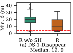
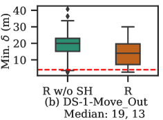
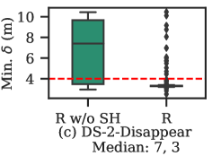
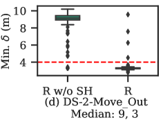
Here we characterize the impact of attacks mounted by RoboTack on the safety potential of the EV with and without the safety hijacker (SH). Our results indicate that the timing of the attack chosen by the SH is critical for causing safety hazards with a high probability of success. In particular, with SH, the number of successful attacks, i.e., forced emergency brakings and crashes, when the vehicle trajectories are hijacked, were up to $\mathbf{5.1\times}$ and $\mathbf{7.2\times}$ higher respectively, than the number of attacks induced at random times using only trajectory hijacking. Attacks that hijacked pedestrian trajectories were $\mathbf{14.8\times}$ and $\mathbf{24\times}$ more successful, respectively. fig. 6 shows the boxplot of the minimum safety potential of the EV measured from the start time of the attack to the end of the driving scenario. Recall that we label as an "accident" any driving scenario that experiences a safety potential of less than 4 meters from the start of the attack to the end of the attack. We determine the presence of forced emergency braking by directly reading the values from the Apollo ADS. In fig. 6, "R w/o SH" stands for "Robotack without SH", and "R" alone stands for the proposed "Robotack" consisting of scenario matcher, trajectory hijacker, and safety hijacker. Thus, the boxplot labeled "R w/o SH" indicates that RoboTack launched a trajectory-hijacking-attack on the EV without SH (random timing), whereas "R" indicates that RoboTack used the safety hijacker’s decided timing to launch a trajectory-hijacking-attack. We omit figures for the Move_In attack vector because in those scenarios the attacks did not reduce the $\delta$ but caused emergency braking only. The improvements of "R" on attack success-rate over "R w/o SH" are as follows.

DS-1-Disappear. RoboTack caused $7.2\times$ more crashes (31.7% vs. 4.4%). In addition, we observed that RoboTack caused $4.6\times$ more emergency braking (53.5% vs. 11.6%).

DS-1-Move_Out. RoboTack caused $6.2\times$ more crashes (17.3% vs. 2.8%). In addition, we observed that RoboTack caused $5.1\times$ more emergency braking (37.3% vs. 7.3%).

DS-2-Disappear. RoboTack caused $7.9\times$ more crashes (82.6% vs. 10.4%). In addition, we observed that RoboTack caused $2.4\times$ more emergency braking (94.4% vs. 39.4%).

DS-2-Move_Out. RoboTack caused $24\times$ more crashes (84.1% vs. 3.5%). In addition, we observed that RoboTack caused $14.8\times$ more emergency braking (97.8% vs. 6.6%).

DS-3-Move_In. RoboTack caused $1.9\times$ more emergency brakings (94.6% vs. 50%). A comparison of the number of crashes would not apply, as there was no real obstacle to crash.

DS-4-Move_In. RoboTack caused $1.6\times$ more emergency braking (78.5% vs 48.1%). A comparison of the number of crashes would not apply, as there was no real obstacle to crash.

Summary. In 1702 experiments (851 "R w/o SH", 851 "R") across all combinations of scenarios and attack vectors, RoboTack (R) resulted in 640 EBs (75.2%) over 851 "R" experiments. In comparison, RoboTack without SH (R w/o SH) resulted in only 230 EBs (27.0%) over 851 "R w/o SH" experiments. RoboTack (R) resulted in 299 crashes (52.6%) over 568 "R" experiments excluding DS-3 and DS-4 with Move_In attacks, while RoboTack without SH (R w/o SH) results in only 29 (5.1%) crashes over the 568 "R w/o SH" experiments excluding DS-3 and DS-4 with Move_In attacks.

Figure 6: Impact of attacks. $\delta$: Safety potential. ‘R’: Robotack. ‘R w/o SH’: Robotack without safety hijacker. Dashed red line: Safety potential $\delta=4$ meters.

Figure 7: Time-steps $K^{\prime}$ required to move object in/out by $\Omega$ (a) on vehicle, (b) on pedestrian.

VI-E Evading Attack Detection

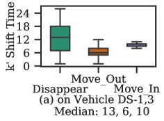
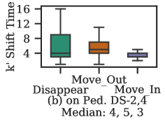
Recall that the trajectory hijacker actively perturbs the estimated trajectory for only $K^{\prime}\ll K$ time-steps to shift the object position laterally at most by $\Omega$, and it maintains the trajectory of the object for the next $K-K^{\prime}$ time-steps, where $K$ is the total number of time-steps for which the attack must be active from start to end. Note that RoboTack perturbs images for all $K$ time-steps. However, RoboTack modifies the image to change the trajectory for only $K^{\prime}$ time-steps, whereas for $K-K^{\prime}$ time-steps, it maintains the faked trajectory.

fig. 7(a) and (b) characterize $K^{\prime}$ for different scenarios and attack vectors. We observed that Move_Out and Move_In scenarios required a smaller $K^{\prime}$ in order to change the object position to the desired location than the Disappear attack vector did. Furthermore, changing of a pedestrian’s location required smaller $K^{\prime}$ than changing of a vehicle’s location.

In those $K^{\prime}$ time-steps, the disparity between between the Kalman filter’s and the object detector’s output is not flagged as evidence of an attack because it is within one standard deviation of the characterized mean during normal situation.

VI-F Characterizing Safety Hijacker Performance

Here we characterize the performance of our neural network and its impact on the malware’s ability to cause a safety hazard. For lack of space, we discuss results only for Move_Out.

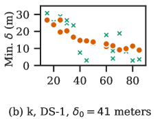
fig. 8(b) shows a plot of the predicted value of the safety potential (using the NN) and the ground-truth value of the safety potential after the attack, as obtained from our experiments. We observe that the predicted value is close to the ground-truth value of the safety potential after the attack. On average, across all driving scenarios, NN’s prediction of the safety potential after the attack was within 5m and 1.5m of the ground-truth values for vehicles and pedestrians, respectively.

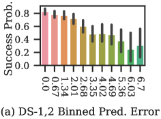
fig. 8(a) shows a plot of the probability of success (i.e., of the malware’s ability to cause a safety hazard) on the y-axis with increasing NN prediction error probability on the x-axis. We find that the success probability goes down as the prediction error of the safety potential (using NN) increases. However, as stated earlier, our NN’s prediction errors are generally small.

VII Related Work

Security attacks. AVs are notoriously easy to hack into due to i) easy physical and software access, ii) the large attack vectors available to the adversary because of the complexity and heterogeneity of the software and hardware, and iii) the lack of robust methods for attack detection. Hence, the insecurity of autonomous vehicles poses one of the biggest threats to their safety and thus to their successful deployment on the road.

Gaining access to AVs. Hackers can gain access to the ADS by hacking existing software and hardware vulnerabilities. For example, research [29, 26] has shown that an adversary can gain access to the ADS and launch cyber attacks by hacking vehicle-to-vehicle (V2V) and vehicle-to-infrastructure (V2I) communication channels [39], over-the-air software update mechanisms used by manufacturers [40], electronic component units (ECUs) [26], infotainment systems [30], and CAN buses [41]. Another way of hacking an ADS is to use hardware-based malware, which can be implanted during the supply chain of AVs or simply by gaining physical access to the vehicle [26]. In this work, we show an attack approach that can masquerade as noise or faults and that can be implanted as malware in either software or hardware.

Adversarial machine learning and sensor attacks in AVs. A comparison with the current state-of-the-art adversarial ML-based attacks is provided in section I.

Figure 8: (a) NN binned prediction error for DS-1, DS-2 Move_Out attack. (b) DS-1 Move_Out attack, NN safety potential prediction. $\times$: ground-truth. $\bullet$: predicted. $k$: $\#$ of attacks. $\delta_{0}$: starting safety potential.

Our attack. We find that none of the above work mentioned attacks geared toward i) evading detection by an IDS or ii) explicitly targeting the safety of the vehicles. In contrast, RoboTack is the first attack approach that has been demonstrated on production ADS software with multiple sensors (GPS, IMU, cameras, LiDAR) to achieve both objectives by attacking only one sensor (the camera).

VIII Conclusion & Future Work

In this work, we present RoboTack, smart malware that strategically attacks autonomous vehicle perception systems to put the safety of people and property at risk. The goal of our research is to highlight the need to develop more secure AV systems by showing that the adversary can be highly efficient in targeting AV safety (e.g., cause catastrophic accidents with high probability) by answering the question of how, when and what to attack. We believe that the broader implications of our research are: (i) Knowledge gathered from this type of study can be used to identify flaws in the current ADS architecture (e.g., vulnerability in Kalman filters to adversarial noise) which can be used to drive future enhancements. (ii) Guide the development of countermeasures. (iii) Looking forward we believe these kinds of attacks can be fully automated and deployed as a new generation of malware.

The design of countermeasures is the subject of our future work. Existing literature has shown a large number of adversarial attacks on these models (e.g., object detection models and Kalman filters). Therefore, we are investigating a broader solution that can dynamically and adaptively tune the parameters of the perception system (i.e., parameters used in object detection, Hungarian matching algorithm and Kalman filters) to reduce their sensitivity to noise and thus, mitigate most of these adversarial attacks.

References

- [1] M. Gerla, E. K. Lee, G. Pau, and U. Lee, “Internet of Vehicles: From Intelligent Grid to Autonomous Cars and Vehicular Clouds,” in Proceedings of 2014 IEEE World Forum on Internet of Things (WF-IoT), Mar 2014, pp. 241–246.
- [2] S. Jha, S. S. Banerjee, J. Cyriac, Z. T. Kalbarczyk, and R. K. Iyer, “AVFI: Fault Injection for Autonomous Vehicles,” in Proceedings of 2018 48th Annual IEEE/IFIP International Conference on Dependable Systems and Networks Workshops (DSN-W), pp. 55–56.
- [3] S. S. Banerjee, S. Jha, J. Cyriac, Z. T. Kalbarczyk, and R. K. Iyer, “Hands off the wheel in autonomous vehicles?: A systems perspective on over a million miles of field data,” in Proceedings of 2018 48th Annual IEEE/IFIP International Conference on Dependable Systems and Networks (DSN). IEEE, 2018.
- [4] S. Jha, T. Tsai, S. Hari, M. Sullivan, Z. Kalbarczyk, S. W. Keckler, and R. K. Iyer, “Kayotee: A Fault Injection-based System to Assess the Safety and Reliability of Autonomous Vehicles to Faults and Errors,” in Third IEEE International Workshop on Automotive Reliability & Test. IEEE, 2018.
- [5] C. Hutchison, M. Zizyte, P. E. Lanigan, D. Guttendorf, M. Wagner, C. Le Goues, and P. Koopman, “Robustness testing of autonomy software,” in 2018 IEEE/ACM 40th International Conference on Software Engineering: Software Engineering in Practice Track (ICSE-SEIP). IEEE, 2018, pp. 276–285.
- [6] S. Jha, S. Banerjee, T. Tsai, S. K. S. Hari, M. B. Sullivan, Z. T. Kalbarczyk, S. W. Keckler, and R. K. Iyer, “ML-Based Fault Injection for Autonomous Vehicles: A Case for Bayesian Fault Injection ,” in Proceedings of 2019 49th Annual IEEE/IFIP International Conference on Dependable Systems and Networks (DSN), June 2019, pp. 112–124.
- [7] P. Koopman, U. Ferrell, F. Fratrik, and M. Wagner, “A safety standard approach for fully autonomous vehicles,” in International Conference on Computer Safety, Reliability, and Security. Springer, 2019, pp. 326–332.
- [8] B. C. Csáji et al., “Approximation with artificial neural networks,” Faculty of Sciences, Etvs Lornd University, Hungary, vol. 24, no. 48, p. 7, 2001.
- [9] Baidu, “Apollo Open Platform,” http://apollo.auto.
- [10] LG Electronics, “LGSVL Simulator,” https://www.lgsvlsimulator.com/, 2018.
- [11] Y. Cao, C. Xiao, D. Yang, J. Fang, R. Yang, M. Liu, and B. Li, “Adversarial Objects Against LiDAR-Based Autonomous Driving Systems,” arXiv preprint arXiv:1907.05418, 2019.
- [12] A. Boloor, K. Garimella, X. He, C. Gill, Y. Vorobeychik, and X. Zhang, “Attacking Vision-based Perception in End-to-End Autonomous Driving Models,” arXiv preprint arXiv:1910.01907, 2019.
- [13] K. Eykholt, I. Evtimov, E. Fernandes, B. Li, A. Rahmati, C. Xiao, A. Prakash, T. Kohno, and D. Song, “Robust Physical-World Attacks on Deep Learning Models,” arXiv preprint arXiv:1707.08945, 2017.
- [14] J. Lu, H. Sibai, and E. Fabry, “Adversarial Examples that Fool Detectors,” arXiv preprint arXiv:1712.02494, 2017.
- [15] Y. Jia, Y. Lu, J. Shen, Q. A. Chen, Z. Zhong, and T. Wei, “Fooling Detection Alone is Not Enough: First Adversarial Attack Against Multiple Object Tracking,” 2019.
- [16] J. Lu, H. Sibai, E. Fabry, and D. Forsyth, “No Need to Worry About Adversarial Examples in Object Detection in Autonomous Vehicles,” arXiv preprint arXiv:1707.03501, 2017.
- [17] K. J. Åström and T. Hägglund, PID Controllers: Theory, Design, and Tuning vol. 2. Instrument Society of America Research Triangle Park, NC, 1995.
- [18] W. Luo, X. Zhao, and T. Kim, “Multiple Object Tracking: A Review,” CoRR, abs/1409.7618, 2014. [Online]. Available: http://arxiv.org/abs/1409.7618
- [19] J. Redmon and A. Farhadi, “YOLOv3: An Incremental Improvement,” arXiv preprint arXiv:1804.02767, 2018.
- [20] S. Ren, K. He, R. Girshick, and J. Sun, “Faster R-CNN: Towards Real-Time Object Detection with Region Proposal Networks ,” in Proceedings of Advances in Neural Information Processing Systems, 2015, pp. 91–99.
- [21] G. Welch, G. Bishop et al., An Introduction to the Kalman Filter. Los Angeles, CA, 1995.
- [22] C. Huang, B. Wu, and R. Nevatia, “Robust Object Tracking by Hierarchical Association of Detection Responses,” in Proceedings of European Conference on Computer Vision. Springer, 2008, pp. 788–801.
- [23] S. M. Erlien, “Shared Vehicle Control Using Safe Driving Envelopes for Obstacle Avoidance and Stability,” Ph.D. dissertation, Stanford University, 2015.
- [24] J. Suh, B. Kim, and K. Yi, “Design and Evaluation of a Driving Mode Decision Algorithm for Automated Driving Vehicle on a Motorway,” IFAC-PapersOnLine, vol. 49, no. 11, pp. 115–120, 2016.
- [25] K.-T. Cho and K. G. Shin, “Fingerprinting Electronic Control Units for Vehicle Intrusion Detection,” in Proceedings of 25th USENIX Security Symposium, 2016, pp. 911–927.
- [26] K. Koscher, A. Czeskis, F. Roesner, S. Patel, T. Kohno, S. Checkoway, D. McCoy, B. Kantor, D. Anderson, H. Shacham et al., “Experimental Security Analysis of a Modern Automobile,” in Proceedings of 2010 IEEE Symposium on Security and Privacy. IEEE, 2010, pp. 447–462.
- [27] D. Rezvani, “Hacking Automotive Ethernet Cameras,” Publisher: https://argus-sec.com/hacking-automotive-ethernet-cameras/, 2018.
- [28] “IEEE 802.1: 802.1ba - Audio Video Bridging (AVB) Systems,” Publisher: http://www.ieee802.org/1/pages/802.1ba.html, (Accessed on 12/12/2019).
- [29] Z. Winkelman, M. Buenaventura, J. M. Anderson, N. M. Beyene, P. Katkar, and G. C. Baumann, “When Autonomous Vehicles Are Hacked, Who Is Liable?” RAND Corporation, Tech. Rep., 2019.
- [30] T. Lin and L. Chen, “Common Attacks Against Car Infotainment systems,” https://events19.linuxfoundation.org/wp-content/uploads/2018/07/ALS19-Common-Attacks-Against-Car-Infotainment-Systems.pdf, 2019.
- [31] O. Pfeiffer, “Implementing Scalable CAN Security with CANcrypt,” Embedded Systems Academy, 2017.
- [32] K. Manandhar, X. Cao, F. Hu, and Y. Liu, “Detection of Faults and Attacks Including False data Injection Attack in Smart Grid Using Kalman Filter,” IEEE Transactions on Control of Network Systems, vol. 1, no. 4, pp. 370–379, 2014.
- [33] Baidu, “Apollo 5.0,” https://github.com/ApolloAuto/apollo.
- [34] LG Electronics, “Modified Apollo 5.0,” https://github.com/lgsvl/apollo-5.0.
- [35] “Unity Engine,” http://unity.com.
- [36] J. Gregory, Game engine architecture. AK Peters/CRC Press, 2017.
- [37] “The config file specifying these sensor parameters can be accessed at,” https://www.lgsvlsimulator.com/docs/apollo5-0-json-example/.
- [38] NEOUSYS, “Nuvo-6108GC GPU Computing Platform | NVIDIA RTX 2080-GTX 1080TI-TITANX,” https://www.neousys-tech.com/en/product/application/gpu-computing/nuvo-6108gc-gpu-computing.
- [39] I. A. Sumra, I. Ahmad, H. Hasbullah et al., “Classes of attacks in VANET,” in Proceedings of 2011 Saudi International Electronics, Communications and Photonics Conference (SIECPC). IEEE, 2011, pp. 1–5.
- [40] A. Sampath, H. Dai, H. Zheng, and B. Y. Zhao, “Multi-channel Jamming Attacks using Cognitive Radios,” in Proceedings of 2007 16th International Conference on Computer Communications and Networks. IEEE, 2007, pp. 352–357.
- [41] E. Yağdereli, C. Gemci, and A. Z. Aktaş, “A Study on Cyber-Security of Autonomous and Unmanned Vehicles,” The Journal of Defense Modeling and Simulation, vol. 12, no. 4, pp. 369–381, 2015.