CoReNet: Coherent 3D scene reconstruction from a single RGB image

Abstract

Advances in deep learning techniques have allowed recent work to reconstruct the shape of a single object given only one RBG image as input. Building on common encoder-decoder architectures for this task, we propose three extensions: (1) ray-traced skip connections that propagate local 2D information to the output 3D volume in a physically correct manner; (2) a hybrid 3D volume representation that enables building translation equivariant models, while at the same time encoding fine object details without an excessive memory footprint; (3) a reconstruction loss tailored to capture overall object geometry. Furthermore, we adapt our model to address the harder task of reconstructing multiple objects from a single image. We reconstruct all objects jointly in one pass, producing a coherent reconstruction, where all objects live in a single consistent 3D coordinate frame relative to the camera and they do not intersect in 3D space. We also handle occlusions and resolve them by hallucinating the missing object parts in the 3D volume. We validate the impact of our contributions experimentally both on synthetic data from ShapeNet as well as real images from Pix3D. Our method improves over the state-of-the-art single-object methods on both datasets. Finally, we evaluate performance quantitatively on multiple object reconstruction with synthetic scenes assembled from ShapeNet objects.

1 Introduction

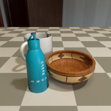
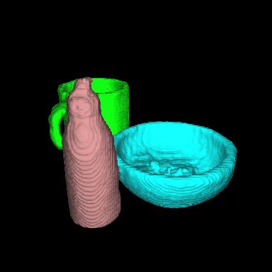
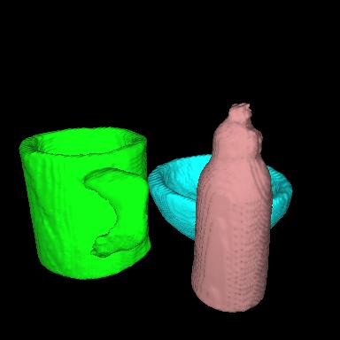
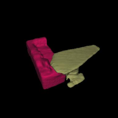
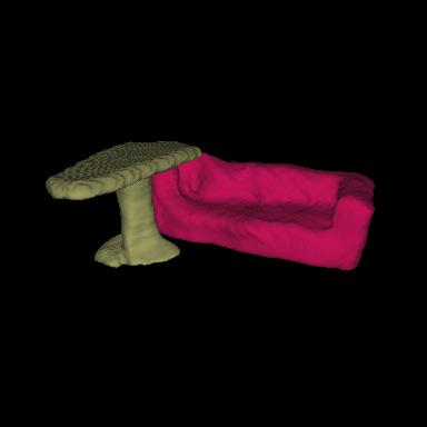
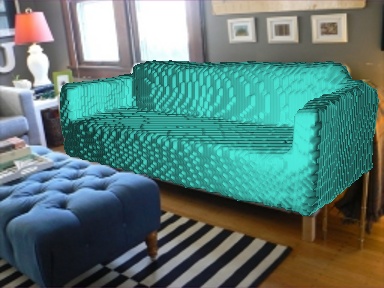
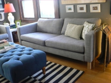
3D reconstruction is key to genuine scene understanding, going beyond 2D analysis. Despite its importance, this task is exceptionally hard, especially in its most general setting: from one RGB image as input. Advances in deep learning techniques have allowed recent work [25, 6, 47, 33, 35, 30, 45, 7, 10, 48] to reconstruct the shape of a single object in an image.

Figure 1: 3D reconstructions from a single RGB image, produced by our model. Left: Coherent reconstruction of multiple objects in a synthetic scene (shown from a view matching the input image, and another view). We reconstruct all objects in their correct spatial arrangement in a common coordinate frame, enforce space exclusion, and hallucinate occluded parts. Right: Reconstructing an object in a real-world scene. The top image shows the reconstruction overlaid on the RGB input. The bottom row shows the input next to two other views of the reconstruction.

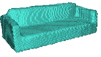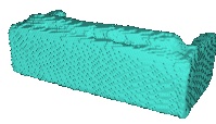In this paper, we first propose several improvements for the task of reconstructing a single object. As in [10, 50], we build a neural network model which takes a RGB input image, encodes it and then decodes it into a reconstruction of the full volume of the scene. We then extract object meshes in a second stage. We extend this simple model with three technical contributions: (1) Ray-traced skip connections as a way to propagate local 2D information to the output 3D volume in a physically correct manner (sec. 3.3). They lead to sharp reconstruction details because visible object parts can draw information directly from the image; (2) A hybrid 3D volume representation that is both regular and implicit (sec. 3.1). It enables building translation equivariant 3D models using standard convolutional blocks, while at the same time encoding fine object details without an excessive memory footprint. Translation equivariance is important for our task, since objects can appear anywhere in space; (3) A reconstruction training loss tailored to capture overall object geometry, based on a generalization of the intersection-over-union metric (IoU) (sec. 3.4). Note that our model reconstructs objects at the pose (translation, rotation, scale) seen from the camera, as opposed to a canonical pose in many previous works [7, 10, 25, 50].

We validate the impact of our contributions experimentally on synthetic data from ShapeNet [4] (sec. 4.1) as well as real images from Pix3D [42] (sec 4.2). The experiments demonstrate that (1) our proposed ray-traced skip connections and IoU loss improve reconstruction performance considerably; (2) our proposed hybrid volume representation enables to reconstruct at resolutions higher than the one used during training; (3) our method improves over the state-of-the-art single-object 3D reconstruction methods on both ShapeNet and Pix3D datasets.

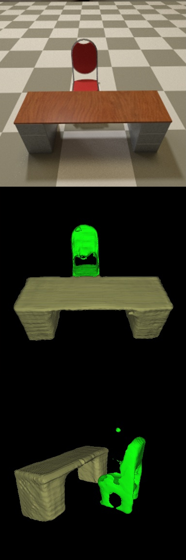
In the second part of this paper, we address the harder task of reconstructing scenes consisting of spatial arrangements of multiple objects. In addition to the shape of individual objects at their depicted pose, we also predict the semantic class of each object. We focus on coherent reconstruction in this scenario, where we want to (1) reconstruct all objects and the camera at their correct relative pose in a single consistent 3D coordinate frame, (2) detect occlusions and resolve them fully, hallucinating missing parts (e.g. a chair behind a table), and (3) ensure that each point in the output 3D space is occupied by at most one object (space exclusion constraint). We achieve this through a relatively simple modification of our single-object pipeline. We predict a probability distribution over semantic classes at each point in the output 3D space and we make the final mesh extraction step aware of this.

The technical contributions mentioned above for the single-object case are even more relevant for reconstructing scenes containing multiple objects. Ray-traced skip connections allow the model to propagate occlusion boundaries and object contact points detected on the 2D image into 3D, and to also understand the depth relations among objects locally. The IoU loss teaches our model to output compact object reconstructions that do not overlap in 3D space. The hybrid volume representation provides a fine discretization resolution, which can compensate for the smaller fraction of the scene volume allocated to each object in comparison to the single object case.

We experimentally study our method’s performance on multiple object reconstruction with synthetic scenes assembled from ShapeNet objects (sec. 4.3). We validate again the impact of our technical contributions, and study the effect of the degree of object occlusion, distance to the camera, number of objects in the scene, and their semantic classes. We observe that ray-traced skip connections and the IoU loss bring larger improvements than in the single object case. We show that our model can handle multiple object scenes well, losing only a fraction of its performance compared to the single object case.

Finally, we study the effect of image realism on reconstruction performance both in the single-object (sec. 4.1) and multi-object (sec. 4.3) cases. We render our images with either (1) local illumination against uniform background like most previous works [25, 47, 33, 45, 7, 10] or (2) a physically-based engine [32], adding global illumination effects, such as shadows and reflections, non-trivial background, and complex lighting from an environment map and finite extent light sources. We publicly release these images, our models, and scene layouts [1].

2 Related work

Single object reconstruction.

In the last few years there has been a surge of methods for reconstructing the 3D shape of one object from a single RGB image. Many of them [7, 10, 48, 50, 51] employ voxel grids in their internal representation, as they can be handled naturally by convolutional neural networks. Some works have tried to go beyond voxels: (1) by using a differentiable voxels-to-mesh operation [21]; (2) by producing multiple depth-maps and/or silhouettes from fixed viewpoints that can be subsequently fused [38, 35, 33, 52]; (3) by operating on point clouds [8, 24], cuboidal primitives [45, 30], and even directly on meshes [47, 5]. A recent class of methods [31, 25, 6] use a continuous volume representation through implicit functions. The model receives a query 3D point as part of its input and returns the occupancy at that point.

We build on principles from these works and design a new type of hybrid representation that is both regular like voxels and continuous like implicit functions (sec. 3.1). We also address more complex reconstruction tasks: we reconstruct objects in the pose as depicted in the image and we also tackle scenes with multiple objects, predicting the semantic class of each object. Finally, we experiment with different levels of rendering realism.

Multi-object reconstruction.

IM2CAD [15] places multiple CAD models from a database in their appropriate position in the scene depicted in the input image. It only reconstructs the pose of the objects and copies over their whole CAD models, without trying to reconstruct their particular 3D shapes as they appear in the input image. 3D-RCNN [18] learns a per-class linear shape basis from a training dataset of 3D models. It then uses a render-and-compare approach to fit the coefficients of this basis to objects detected in the test image. This method only outputs 3D shapes that lie on a simple linear subspace spanning the training samples. Instead our model can output arbitrary shapes, and the mapping between image appearance and shape is more complex as it is modeled by a deep neural network. Tulsiani et. al. [44] first detects object proposals [53] and then reconstructs a pose and a voxel grid for each, based on local features for the proposal and a global image descriptor. Mesh-RCNN [9] extends Mask-RCNN [13] to predict a 3D mesh for each detected object in an image. It tries to predict the objects positions in the image plane correctly, but it cannot resolve the fundamental scale/depth ambiguity along the Z-axis.

All four methods [15, 18, 44, 9] first detect objects in the 2D image, and then reconstruct their 3D shapes independently. Instead, we reconstruct all objects jointly and without relying on a detection stage. This allows us to enforce space exclusion constraints and thus produce a globally coherent reconstruction.

The concurrent work [29] predicts the 3D pose of all objects jointly (after 2D object detection). Yet, it still reconstructs their 3D shape independently, and so the reconstructions might overlap in 3D space. Moreover, in contrast to [29, 44, 15, 18] our method is simpler as it sidesteps the need to explicitly predict per-object poses, and instead directly outputs a joint coherent reconstruction.

Importantly, none of these works [15, 18, 9, 29] offers true quantitative evaluation of 3D shape reconstruction on multiple object scenes. One of the main reasons for this is the lack of datasets with complete and correct ground truth data. One exception is [44] by evaluating on SunCG [39], which is now banned. In contrast, we evaluate our method fully, including the 3D shape of multiple objects in the same image. To enable this, we create two new datasets of scenes assembled from pairs and triplets of ShapeNet objects, and we report performance with a full scene evaluation metric (sec. 4.3).

Finally, several works tackle multiple object reconstruction from an RGB-D image [28, 40], exploiting the extra information that depth sensors provides.

Neural scene representations.

Recent works [34, 36, 26, 27, 37, 23] on neural scene representations and neural rendering extract latent representations of the scene geometry from images and share similar insights to ours. In particular, [16, 46] use unprojection, a technique to accumulate latent scene information from multiple views, related to our ray-traced skip connections. Others [34, 37] can also reconstruct (single-object) geometry from one RGB image.

3 Proposed approach

Figure 2: Left: 2D slice of the output grid (yellow points) and a decoder layer grid (blue points). The output grid is offset by $\bar{o}$ from the origin. The decoder grid, which has $k$ times lower resolution, by $k\bar{o}$. Right: Side-cut of our model’s architecture. Ray-traced skip connections (red) propagate data from the encoder to the decoder, $\bar{o}$ is appended to the channels of select decoder layers (green).

For simplicity and compactness of exposition, we present directly our full method, which can reconstruct multiple objects in the same image. Our reconstruction pipeline takes a single RGB image as input and outputs a set of meshes – one for each object in the scene. It is trained to jointly predict the object shapes, their pose relative to the camera, and their class label.

At the core of our pipeline is a neural network model that receives a single RGB image and a set of volume query points as input and outputs a probability distribution over $C$ possible classes at each of these points. One of the classes is void (i.e. empty space), while the rest are object classes, such as chair and table. Predicting normalized distributions creates competition between the classes and forces the model to learn about space exclusion. For single object models, we use two classes (foreground and void, $C=2$).

To create a mesh representation, we first reconstruct a fine discretization of the output volume (sec. 3.5). We query the model repeatedly, at different locations in 3D space, and we integrate the obtained outputs. We then apply marching cubes [20] over the discretization, in a way that enforces the space exclusion constraint. We jitter the query points randomly during training. For single object models, we treat all meshes as parts of one single output object.

3.1 3D volume representation

We want our model to reconstruct the large 3D scene volume at a fine spatial resolution, so we can capture geometric details of individual objects, but without an excessive memory footprint. We also want it to be translation equivariant: if the model sees e.g. chairs only in one corner of the scene during training, it should still be able to reconstruct chairs elsewhere. This is especially important in a multi-object scenario, where objects can appear anywhere in space.

A recent class of models [25, 6, 31] address our first requirement through an implicit volume representation. They input a compact code, describing the volume contents, and a query point. They output the occupancy of the volume at that point. These models can be used for reconstruction by conditioning on a code extracted from an image, but are not translation equivariant by design.

Models based on a voxel grid representation [7, 10] are convolutional in nature, and so address our translation equivariance requirement, but require excessive memory to represent large scenes at fine resolutions (cubic in the number of voxels per dimension).

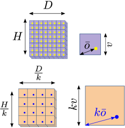
We address both requirements with a new hybrid volume representation and a model architecture based on it. Our model produces a multinomial distribution over the $C$ possible classes on a regular grid of points. The structure of the grid is fixed (i.e. fixed resolution $W{\mkern-2.0mu\times\mkern-2.0mu}H{\mkern-2.0mu\times\mkern-2.0mu}D$ and distance between points $v$), but we allow the grid to be placed at an arbitrary spatial offset $\bar{o}$, smaller than $v$ (fig. 2). The offset value is an input to our model, which then enables fine-resolution reconstruction (see below).

This representation combines the best of voxel grids and implicit volumes. The regular grid structure allows to build a fully convolutional model that is translation equivariant by design, using only standard 3D convolution building blocks. The variable grid offset allows to reconstruct regular samplings of the output volume at any desired resolution (multiple of the model grid’s resolution), while keeping the model memory footprint constant. To do this, we call our model repeatedly with different appropriately chosen grid offsets during inference (sec. 3.5) and integrate the results into a single, consistent, high-resolution output. We sample the full output volume with random grid offsets $\bar{o}$ during training.

3.2 Core model architecture

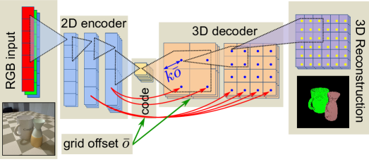
We construct our model on top of an encoder-decoder skeleton (fig. 2). A custom decoder transforms the output of a standard ResNet-50 [14] encoder into a $W{\mkern-2.0mu\times\mkern-2.0mu}H{\mkern-2.0mu\times\mkern-2.0mu}D{\mkern-2.0mu\times\mkern-2.0mu}C$ output tensor – a probability distribution over the $C$ possible classes for each point in the output grid. The decoder operations alternate between upscaling, using transposed 3D convolutions with stride larger than 1, and data mixing while preserving resolution, using 3D convolutions with stride 1.

We condition the decoder on the grid offset $\bar{o}$. We further create ray-traced skip connections that propagate information from the encoder to the decoder layers in a physically accurate manner in sec. 3.3. We inject $\bar{o}$ and the ray-traced skip connections before select data mixing operations.

3.3 Ray traced skip connections

Figure 3: Pixels in the 2D encoder embed local image information, which ray-traced skip connections propagate to all 3D decoder grid points in the corresponding frustum.

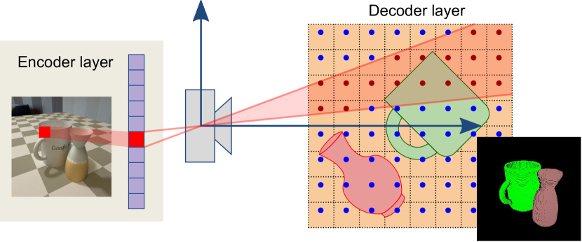
So far we relied purely on the encoder to learn how to reverse the physical process that converts a 3D scene into a 2D image. This process is well understood however [12, 32] and many of its elements have been formalized mathematically. We propose to inject knowledge about it into the model, by connecting each pixel in the input image to its corresponding frustum in the output volume (fig. 3).

We assume for now that the camera parameters are known. We can compute the 2D projection on the image plane of any point in the 3D output volume and we use this to build ray-traced skip connections. We choose a source 2D encoder layer and a target 3D decoder layer. We treat the $W_{e}{\mkern-2.0mu\times\mkern-2.0mu}H_{e}{\mkern-2.0mu\times\mkern-2.0mu}C_{e}$ encoder layer as a $W_{e}{\mkern-2.0mu\times\mkern-2.0mu}H_{e}$ image with $C_{e}$ channels, taken by our camera. We treat the $W_{d}{\mkern-2.0mu\times\mkern-2.0mu}H_{d}{\mkern-2.0mu\times\mkern-2.0mu}D_{d}{\mkern-2.0mu\times\mkern-2.0mu}C_{d}$ decoder layer as a $W_{d}{\mkern-2.0mu\times\mkern-2.0mu}H_{d}{\mkern-2.0mu\times\mkern-2.0mu}D_{d}$ grid of points. We project the decoder points onto the encoder image, then sample it at the resulting 2D coordinates, and finally carry the sampled data over to the 3D decoder. This creates skip connections in the form of rays that start at the camera image plane, pass through the camera pinhole and end at the decoder grid point (fig. 3). We connect several of the decoder layers to the encoder in this manner, reducing the channel count beforehand to $0.75\cdot C_{d}$ by using $1{\mkern-2.0mu\times\mkern-2.0mu}1$ convolutions.

Decoder grid offset.

An important detail is how to choose the parameters of the decoder layer’s grid. The resolution is determined by the layer itself (i.e. $W_{d}{\mkern-2.0mu\times\mkern-2.0mu}H_{d}{\mkern-2.0mu\times\mkern-2.0mu}D_{d}$). It has $k$ times lower resolution than the output grid (by design). We choose $v_{d}=kv$ for distance between the grid points and $\bar{o_{d}}=k\bar{o}$ for grid offset (fig. 2). This makes the decoder grid occupy the same space as the final output grid and respond to changes in the offset $\bar{o}$ in a similar way. In turn, this aids implicit volume reconstruction in sec. 3.5 with an additional parallax effect.

Obtaining camera parameters.

Ray-traced skip connections rely on known camera parameters. In practice, the intrinsic parameters are often known. For individual images, they can be deduced from the associated metadata (e.g. EXIF in JPEGs). For 3D datasets such as Pix3D [42] and Matterport3D [3] they are usually provided. When not available, we can assume default intrinsic parameters, leading to still plausible 3D reconstructions (e.g. correct relative proportions but wrong global object scale). The extrinsic parameters in contrast are usually unknown. We compensate for this by reconstructing relative to the camera rather than in world space, resulting in an identity extrinsic camera matrix.

3.4 IoU training loss

The output space of our model is a multinomial distribution over the $C$ possible classes (including void), for each point in 3D space. This is analog to multi-class recognition in 2D computer vision and hence we could borrow the categorical cross-entropy loss common in those works [14, 13]. In our case, most space in the output volume in empty, which leads to most predicted points having the void label. Moreover, as only one object can occupy a given point in space, then all but one of the $C$ values at a point will be $0$. This leads to even more sparsity. A better loss, designed to deal with extreme class imbalance, is the focal loss [22].

Both categorical cross-entropy and the focal loss treat points as a batch of independent examples and average the individual losses. They are not well suited for 3D reconstruction, as we care more about overall object geometry, not independent points. The 3D IoU metric is better suited to capture this, which inspired us to create a new IoU loss, specifically aiming to minimize it. Similar losses have been successfully applied to 2D image segmentation problems [41, 2].

We generalize IoU, with support for continuous values and multiple classes: $$\textit{IoU}_{\textit{g}}(g,p)=\frac{\sum\limits_{i\in G}{\sum\limits_{c=1}^{C-1}{\min(g_{ic},p_{ic})\cdot\mu(g_{ic})}}}{\sum\limits_{i\in G}{\sum\limits_{c=1}^{C-1}{\max(g_{ic},p_{ic})\cdot\mu(g_{ic})}}},\ \ \mu(g_{ic})=\begin{cases}1&,\textrm{if }g_{ic}=1\\ \frac{1}{C-1}&,\textrm{if }g_{ic}=0\end{cases}$$ (1) where $i$ loops over the points in the grid, $c$ – over the $C-1$ non-void classes, $g_{ic}\in\{0,1\}$ is the one-hot encoding of the ground truth label, indicating whether point $i$ belongs to class $c$, and $p_{ic}\in[0,1]$ is the predicted probability. $\mu(g_{ic})$ balances for the sparsity due to multiple classes, as $C-1$ values in the ground truth one-hot encoding will be 0.

With two classes (i.e. $C=2$) and binary values for $p$ and $g$, ${\textit{IoU}_{\textit{g}}}$ is equivalent to the intersection-over-union measure. The $\max$ operator acts like logical and, $\min$ like logical or, and $\mu(g_{ic})$ is always one. In the case where there is a single object class to be reconstructed we use $1-{\textit{IoU}_{\textit{g}}}$ as a loss (sec. 4.1). With multiple objects, we combine ${\textit{IoU}_{\textit{g}}}$ with categorical cross entropy into a product (sec. 4.3)

3.5 Mesh reconstruction

Our end-goal is to extract a set of meshes that represent the surface of the objects in the scene. To do this, we first reconstruct an arbitrary fine discretization of the volume, with a resolution that is an integer multiple $n$ of the model’s output resolution. We call the model $n^{3}$ times, each time with a different offset $\bar{o}\in\left\{\frac{0+0.5}{n}v,\frac{1+0.5}{n}v,...,\frac{n-1+0.5}{n}v\right\}^{3}$ and we interleave the obtained grid values. The result is a $nW{\mkern-2.0mu\times\mkern-2.0mu}nH{\mkern-2.0mu\times\mkern-2.0mu}nD{\mkern-2.0mu\times\mkern-2.0mu}C$ discretization of the volume.

We then extract meshes. We break the discretization into $C$ slices of shape $nW{\mkern-2.0mu\times\mkern-2.0mu}nH{\mkern-2.0mu\times\mkern-2.0mu}nD$, one for each class. We run marching cubes [20] with threshold $0.5$ on each slice independently and we output meshes, except for the slice corresponding to the void class. The $0.5$ threshold enforces space exclusion, since at most one value in a probability distribution can be be larger than $0.5$.

4 Experiments

Figure 4: Single object experiments (sec. 4.1). Left: Scenes reconstructed by $h_{7}$, shown from two different viewpoints. Our model handles thin structures and hallucinates invisible back-facing object parts. Right: Scenes reconstructed by $y_{1}$. Despite the low resolution of $y_{1}$ ($32^{3}$, second row), we reconstruct high-quality meshes (first row) by sampling $y_{1}$ with $4^{3}$ grid offsets (see sec. 3).

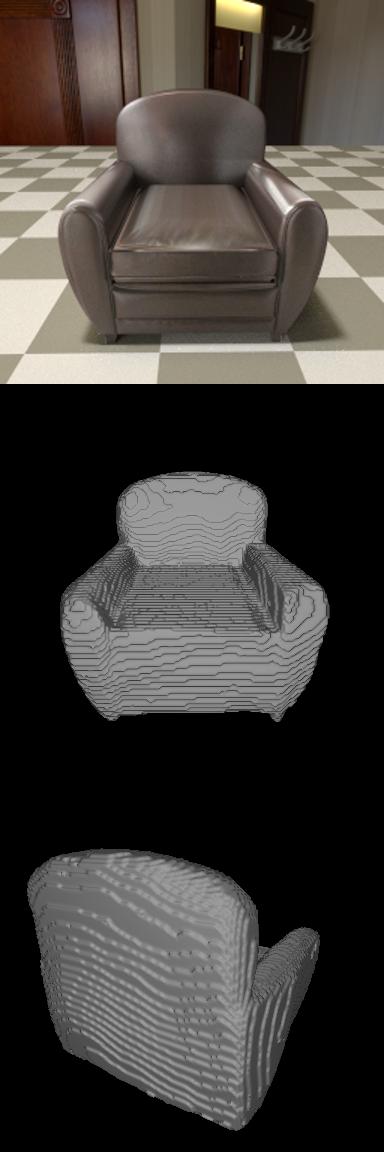
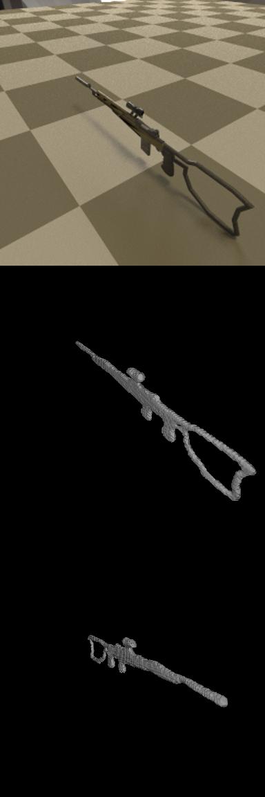
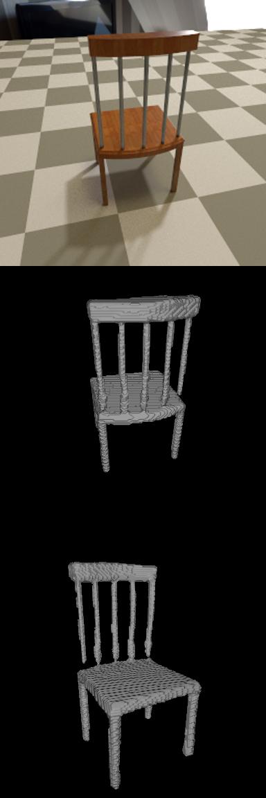
We first present experiments on single object reconstruction on synthetic images from ShapeNet [4] (sec. 4.1) and on real images from Pix3D [42] (sec. 4.2). Then we evaluate performance on multiple object reconstruction in sec. 4.3.

4.1 Single object reconstruction on ShapeNet

Dataset.

We use ShapeNet [4], following the setting of [7]. We consider the same 13 classes, train on 80% of the object instances and test on 20% (the official ShapeNet-trainval and ShapeNet-test splits). We normalize and center each object in the unit cube and render it from 24 random viewpoints, with two levels of photorealism (see inset figure on the right): low realism, using local illumination on a uniform background, with no secondary effects such as shadows and reflections; and high realism, with full global illumination using PBRT’s renderer [32], against an environment map background, and with a ground plane. The low realism setting is equivalent to what was used in previous works [25, 47, 7].

Default settings.

Unless specified otherwise, we train and evaluate at the same grid resolution ($128^{3}$), and we use the same camera parameters in all scenes. We evaluate intersection-over-union as a volumetric metric, reporting mean over the classes (mIoU) as well as the global mean over all object instances. We also evaluate the predicted meshes with the F@1%-score [43] as a surface metric. As commonly done [31, 25, 6], we pre-process the ground-truth meshes to make them watertight and to remove hidden and duplicate surfaces. We sample all meshes uniformly with 100K points, then compute F-score for each class, and finally report the average over classes.

Reconstruction performance.

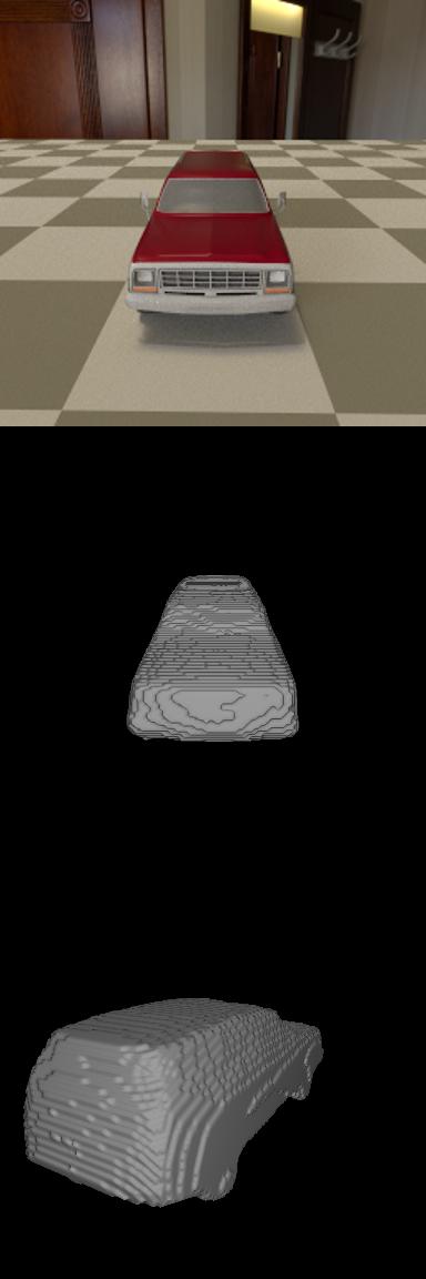
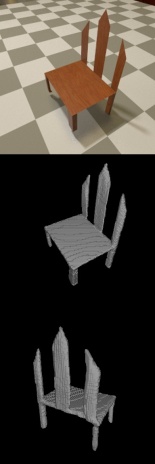
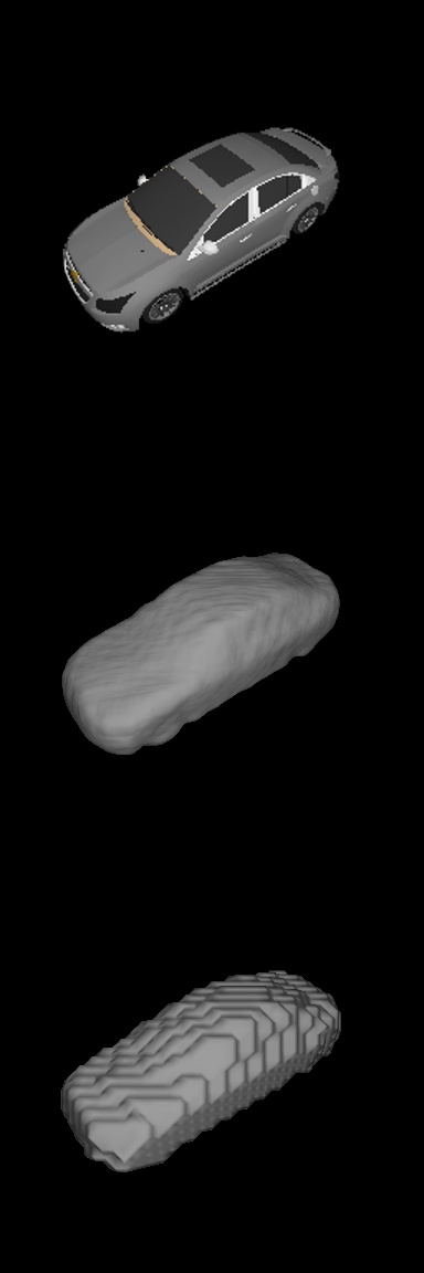
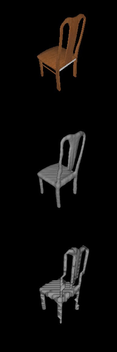
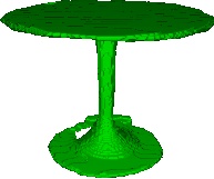
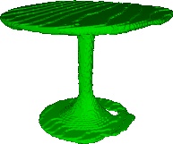
We report the effect of hyper parameters on performance in table 1(a) and show example reconstructions in fig. 4. Ray-traced skip connections improve mIoU by about $5\%$ and F@1% by 10%, in conjunction with any loss. Our IoU loss performs best, followed by focal and categorical cross entropy (Xent). Somewhat surprisingly, results are slightly better on images with high realism, even though they are visually more complex. Shadows and reflections might be providing additional reconstruction cues in this case. Our best model for low realism images is $h_{5}$ and for high realism it is $h_{7}$.

	skip		rea-	IoU
id	conn.	loss	lism	mean	glob.	F@1%
$h_{1}$	No	focal	low	50.8	52.0	45.0
$h_{2}$	No	IoU	low	53.0	53.9	47.8
$h_{3}$	Yes	Xent	low	54.1	55.2	52.9
$h_{4}$	Yes	focal	low	56.6	57.5	54.4
$h_{5}$	Yes	IoU	low	57.9	58.7	57.5
$h_{6}$	Yes	Focal	high	58.1	58.4	57.3
$h_{7}$	Yes	IoU	high	59.1	59.3	59.5

		skip		rea-	IoU
id	data	conn.	loss	lism	mean	glob.
$m_{1}$	pairs	no	focal	high	34.9	46.4
$m_{2}$	pairs	no	IoU	high	33.1	43.4
$m_{3}$	pairs	yes	focal	low	40.4	49.7
$m_{4}$	pairs	yes	IoU	low	41.8	50.6
$m_{5}$	pairs	yes	Xent	high	30.0	43.5
$m_{6}$	pairs	yes	focal	high	42.7	52.4
$m_{7}$	pairs	yes	IoU	high	43.1	52.7
$m_{8}$	tripl.	yes	focal	high	43.0	49.1
$m_{9}$	tripl.	yes	IoU	high	43.9	49.8
$m_{10}$	single	yes	focal	high	43.4	53.9
$m_{11}$	single	yes	IoU	high	46.9	56.4

Table 1: Reconstruction performance in % for (a) our single object experiments on the left, and (b) our multiple object experiments on the right.

Comparison to state-of-the-art.

We compare our models to state-of-the art single object reconstruction methods [25, 50, 7, 47]. We start with an exact comparison to ONN [25]. For this we use the open source implementation provided by the authors to train and test their model on our low-realism images train and test sets. We then use our evaluation procedure on their output predictions. As table 2 shows, ONN achieves $52.6\%$ mIoU on our data with our evaluation (and 51.5% with ONN’s evaluation procedure). This number is expectedly lower than the $57.1\%$ reported in [25] as we ask ONN to reconstruct each shape at the pose depicted in the input image, instead of the canonical pose. From ONN’s perspective, the training set contains 24 times more different shapes, one for each rendered view of an object. Our best model for low-realism renderings $h_{5}$ outperforms ONN on every class and achieves $57.9\%$ mIoU. ONN’s performance is comparable to $h_{2}$, our best model that, like ONN, does not use skip connections.

model	mIoU	airplane	bench	cabinet	car	chair	display	lamp	loudspeaker	rifle	sofa	table	telephone	vessel
$ONN^{*}$	52.6	45.8	45.1	43.8	54.0	58.5	55.4	39.5	57.0	48.0	68.0	50.7	68.3	49.9
$h_{2}$	53.0	46.9	44.3	44.7	56.4	57.4	53.8	35.9	58.1	53.4	67.2	49.7	70.9	49.9
$h_{5}$	57.9	53.0	50.8	50.9	57.3	63.0	57.2	42.1	60.8	64.6	70.6	55.5	73.1	54.0
3D-R2N2	49.3	42.6	37.3	66.7	66.1	43.9	44.0	28.1	61.1	37.5	62.6	42.0	61.1	48.2
Pix2Mesh	48.0	42.0	32.3	66.4	55.2	39.6	49.0	32.3	59.9	40.2	61.3	39.5	66.1	39.7
ONN	57.1	57.1	48.5	73.3	73.7	50.1	47.1	37.1	64.7	47.4	68.0	50.6	72.0	53.0

Table 2: Comparison to state of the art. The first three rows compare ONN [25] to our models $h_{2}$ and $h_{5}$, all trained on our data. The next three rows are taken from [25] and report performance of 3D-R2N2 [7], Pix2Mesh [47], and ONN [25] on their data.

We then compare to 3D-R2N2 [7], Pix2Mesh [47], and again ONN [25], using their mIoU as reported by [25] (table 2). Our model $h_{5}$ clearly outperforms 3D-R2N2 (+$8.6\%$) and Pix2Mesh (+$9.9\%$). It also reaches a slightly better mIoU than ONN (+$0.8\%$), while reconstructing in the appropriate pose for each input image, as opposed to a fixed canonical pose. We also compare on the Chamfer Distance surface metric, implemented exactly as in [25]. We obtain $0.15$, which is better than 3D-R2N2 (0.278), Pix2Mesh (0.216), and ONN (0.215), all compared with the same metric (as reported by [25]).

Finally, we compare to Pix2Vox [50] and its extension Pix2Vox++ [51] (concurrent work to ours). For a fair comparison we evaluate our $h_{5}$ model on a $32^{3}$ grid of points, matching the $32^{3}$ voxel grid output by [50, 51]. We compare directly to the mIoU they report. Our model $h_{5}$ achieves 68.9% mIoU in this case, $+2.8\%$ higher than Pix2Vox (66.1% for their best Pix2Vox-A model) and $+1.9\%$ higher than Pix2Vox++ (67.0% for their best Pix2Vox++/A model).

Reconstructing at high resolutions.

Our model can perform reconstruction at a higher resolution than the one used during training (sec. 3.1). We study this here by reconstructing at $2\times$ and $4\times$ higher resolution. We train one model ($y_{1}$) using a $32^{3}$ grid and one ($y_{2}$) using a $64^{3}$ grid, with ray-traced skip connections, images with low realism, and focal loss. We then reconstruct a $128^{3}$ discretization from each model, by running inference multiple times at different grid offsets (64 and 8 times, respectively, sec. 3.5). At test time, we always measure performance on the $128^{3}$ reconstruction, regardless of training resolution.

Fig. 4 shows example reconstructions. We compare performance to $h_{4}$ from table 1, which was trained with same settings but at native grid resolution $128^{3}$. Our first model (trained on $32^{3}$ and producing $128^{3}$) achieves $53.1\%$ mIoU. The second model (trained on $64^{3}$ and producing $128^{3}$) gets to $56.1\%$, comparable to $h_{4}$ ($56.6\%$). This demonstrates that we can reconstruct at substantially higher resolution than the one used during training.

4.2 Single object reconstruction on Pix3D

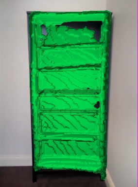
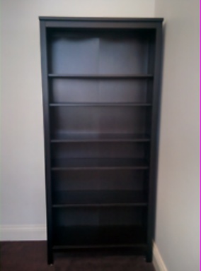
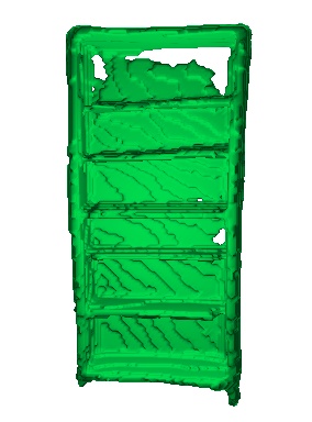
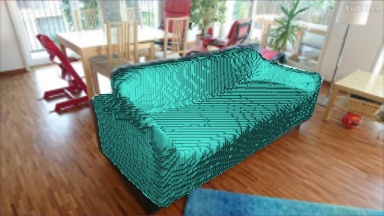
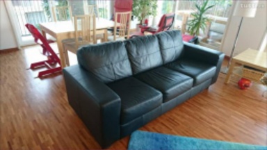
We evaluate the performance of our method on real images using the Pix3D dataset [42], which contains 10069 images annotated with 395 unique 3D models from 9 classes (bed, bookcase, chair, desk, misc, sofa, table, tool, wardrobe). Most of the images are of indoor scenes, with complex backgrounds, occlusion, shadows, and specular highlights.

The images often contain multiple objects, but Pix3D provides annotations for exactly one of them per image. To deal with this discrepancy, we use a single object reconstruction pipeline. At test time, our method looks at the whole image, but we only reconstruct the volume inside the 3D box of the object annotated in the ground-truth. This is similar to how other methods deal with this discrepancy at test time.

Figure 5: Qualitative results on Pix3D. For each example, the large image shows our reconstruction overlaid on the RGB input. The smaller images show the RGB input, and our reconstruction viewed from two additional viewpoints.

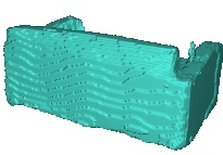
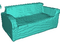Generalization across domains (ShapeNet to Pix3D).

We first perform experiments in the same settings as previous works [7, 42, 50], which train on synthetic images of ShapeNet objects. As they do, we focus on chairs. We train on the high-realism synthetic images from sec. 4.1. For each image we crop out the chair and paste it over a random background from OpenImages [19, 17], a random background from SunDB [49], and a white background. We start from a model pre-trained on ShapeNet ($h_{7}$, sec. 4.1) and continue training on this data.

We evaluate on the 2894 Pix3D images with chairs that are neither occluded nor truncated. We predict occupancy on a $32^{3}$ discretization of 3D space. This is the exact same setting used in [7, 42, 50, 51]. Our model achieves 29.7% IoU, which is higher than Pix2Vox [50] ($28.8\%$, for their best Pix2Vox-A model), the Pix3D method [42] ($28.2\%$, for their best ‘with pose’ model), 3D-R2N2 [7] ($13.6\%$, as reported in [42]), and the concurrent work Pix2Vox++ [51] ($29.2\%$ for their best Pix2Vox++/A model).

This setting is motivated by the fact that most real-world images do not come with annotations for the ground-truth 3D shape of the objects in them. Therefore, it represents the common scenario of training from synthetic data with available 3D supervision.

Fine tuning on real data from Pix3D.

We now consider the case where we do have access to a small set of real-world images with ground-truth 3D shapes for training. For this we use the $S_{1}$ and $S_{2}$ train/test splits of Pix3D defined in [9]. There are no images in common between the test and train splits in both $S_{1}$ and $S_{2}$. Furthermore, in $S_{2}$ also the set of object instances is disjoint between train and test splits. In $S_{1}$ instead, some objects are allowed to be in both the splits, albeit with a different pose and against a different background.

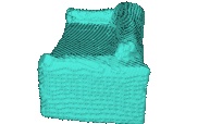
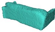
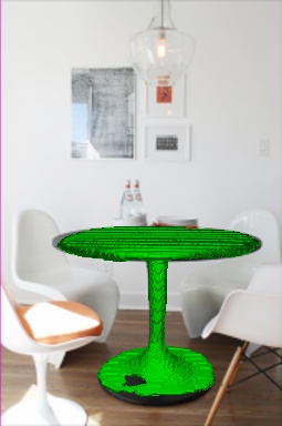
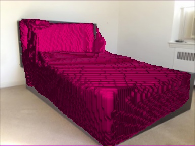
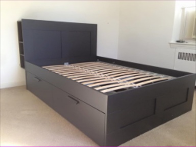
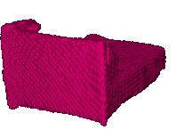
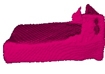
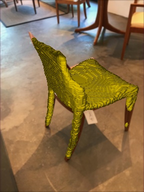
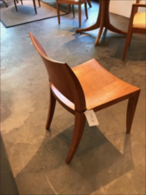
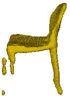
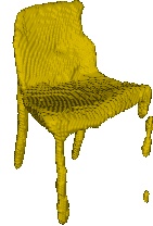
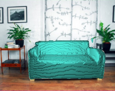
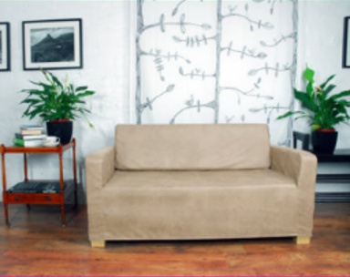
We train two models, one for $S_{1}$ and one for $S_{2}$. In both cases, we start from a model pre-trained on ShapeNet ($h_{7}$) and we then continue training on the respective Pix3D train set. On average over all 9 object classes, we achieve $33.3\%$ mIoU on the test set of $S_{1}$, and $23.6\%$ on the test set of $S_{2}$, when evaluating at $128^{3}$ discretization of 3D space (fig. 5).

As a reference, we compare to a model trained only on ShapeNet. As above, we start from $h_{7}$ and we augment with real-world backgrounds. We evaluate performance on all 9 object classes on the test splits of $S_{1}$ and $S_{2}$. This leads to $20.9\%$ mIoU for S1 and $20.0\%$ for $S_{2}$. This confirms that fine-tuning on real-world data from Pix3D performs better than training purely on synthetic data.

Figure 6: Pairs and triplets reconstructed by $m_{7}$ and $m_{9}$, shown from the camera and from one additional viewpoint. Our model hallucinates the occluded parts and reconstructs all objects in their correct spatial arrangement, in a common coordinate frame.

4.3 Multiple object reconstruction

Datasets and settings.

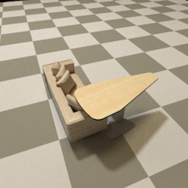
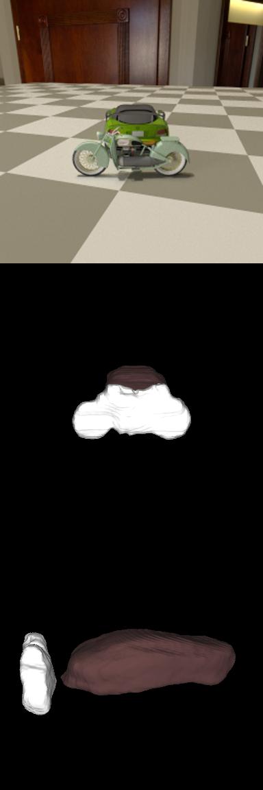
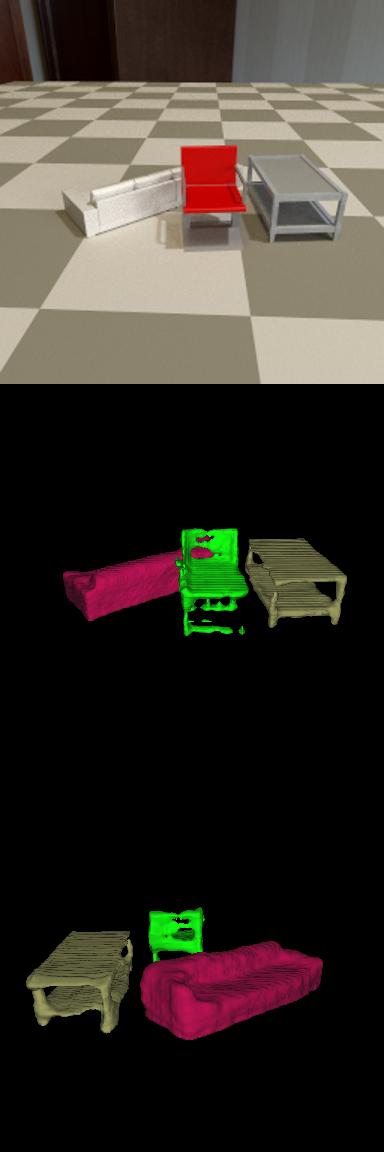
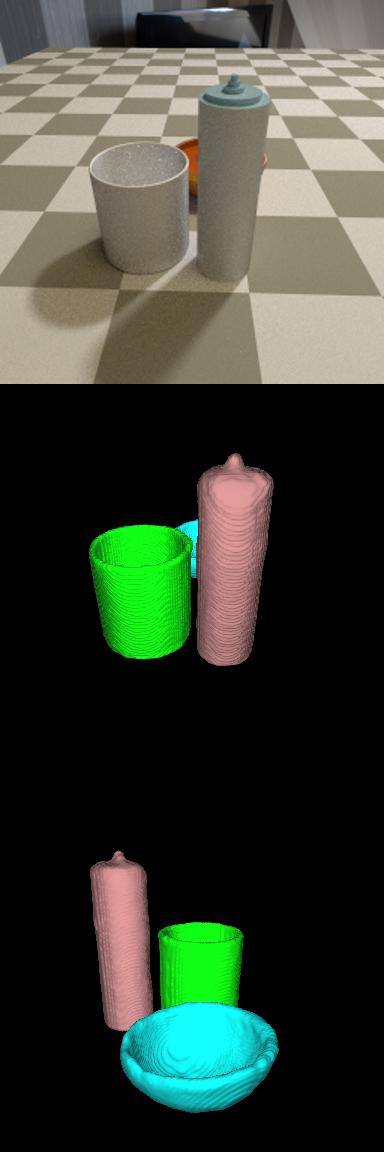
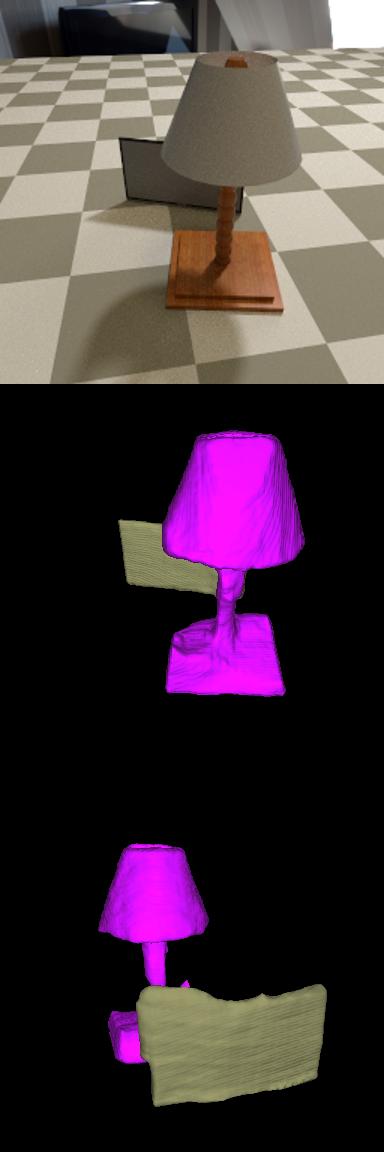
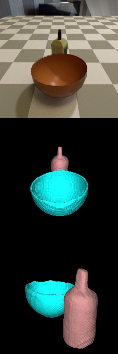
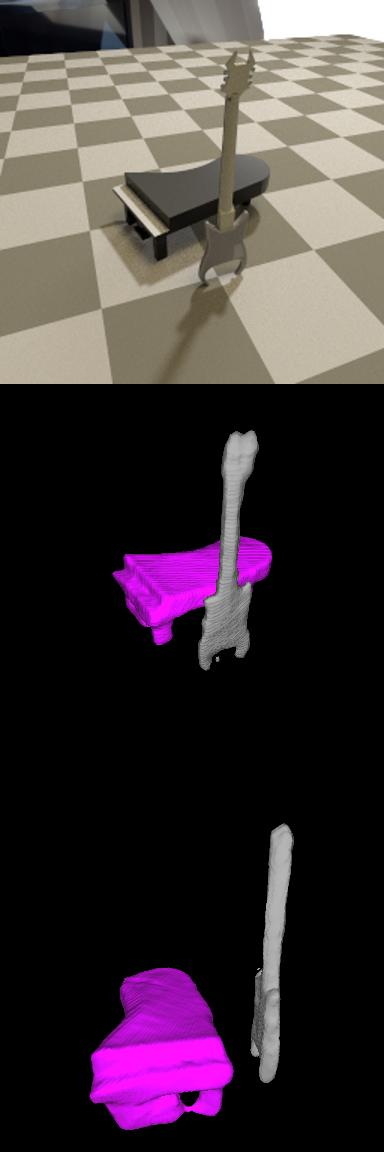
We construct two datasets by assembling objects from ShapeNet. The first is ShapeNet-pairs, with several pairs of object classes: bed-pillow, bottle-bowl, bottle-mug, chair-table, display-lamp, guitar-piano, motorcycle-car. The second is ShapeNet-triplets, with bottle-bowl-mug and chair-sofa-table. We randomly sample the object instances participating in each combination from ShapeNet, respecting its official trainval and test splits. For each image we generate, we random sample two/three object instances, place them at random locations on the ground plane, with random scale and rotation, making sure they do not overlap in 3D, and render the scene from a random camera viewpoint (yaw and pitch). We construct the same number of scenes for every pair/triplet for training and testing. Note how the objects’ scales and rotations, as well as the camera viewpoints, vary between the train and test splits and between images within a split (but their overall distribution is the same). Like the single-object case, the object instances are disjoint in the training and test splits. In total, for pairs we generate 365’600 images on trainval and 91’200 on test; for triplets we make 91’400 on trainval and 22’000 on test.

We perform experiments varying the use of ray-traced skip connections, the image realism, and the loss. Besides categorical cross entropy (Xent) and focal loss, we also combine Xent and ${\textit{IoU}_{\textit{g}}}$ (1) into a product. The IoU part pushes the model to reconstruct full shapes, while Xent pushes it to learn the correct class for each 3D point. We train on the train and val splits together, and test on the test split, always with grid resolution $128^{3}$.

Reconstruction performance.

Table 1(b) summarizes our results, including also multi-class reconstruction of images showing a single ShapeNet object for reference (bottom row, marked ‘single’). We show example reconstructions in fig. 6. On ShapeNet-pairs, using ray-traced skip connections improves mIoU substantially (by $8-10\%$), in conjunction with any loss function. The improvement is twice as large than in the single object case (table 1), confirming that ray-traced skip connections indeed help more for multiple objects. They allow the model to propagate occlusion boundaries and object contact points detected on the 2D image into 3D, and also to understand the depth relations among objects locally. When using skip connections, our IoU loss performs best, followed closely by the focal loss. The cross-entropy loss underperforms in comparison ($-13\%$ mIoU). As with the single-object case, results are slightly better on higher image realism.

Importantly, we note that performance for pairs/triplets is only mildly lower than for the easier single-object scenario. To investigate why, we compare the single-object models $m_{11}$ and $h_{7}$ from table 1. They differ in the number of classes they handle (14 for $m_{11}$, 2 for $h_{7}$) but have otherwise identical settings. While the difference in their mean IoUs is $12\%$ ($46.9\%$ vs. $59.1\%$), their global IoUs are close ($56.4\%$ vs. $59.3\%$). Hence, our model is still good at reconstructing the overall shapes of objects, but makes some mistakes in assigning the right class.

Finally, we note that reconstruction is slightly better overall for triplets rather than for pairs. This is due to the different classes involved. On pairs composed of the same classes appearing in the triplets, results are better for pairs.

In conclusion, these results confirm that we are able to perform 3D reconstruction in the harder multiple object scenario.

Figure 7: mIoU vs. object occlusion and depth.

Occlusion and distance.

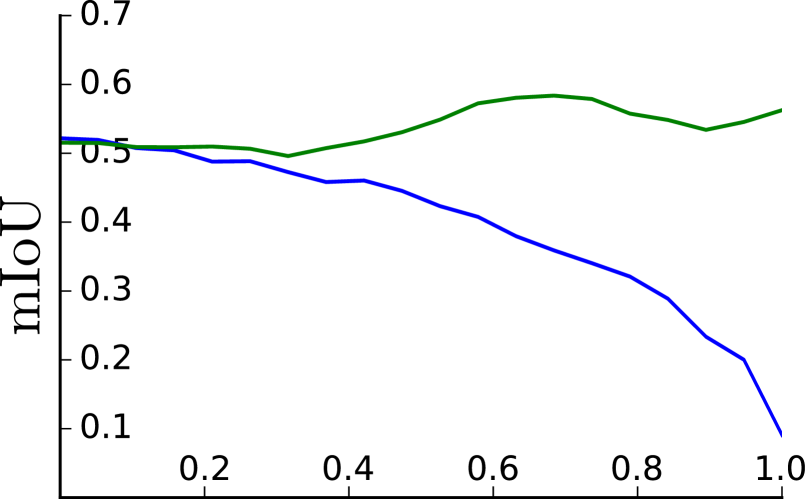
In fig. 7, we break down the performance (mIoU) of $m_{7}$ by the degree of object occlusion (blue), and also by the object depth for unoccluded objects (i.e. distance to the camera, green). The performance gracefully degrades as occlusion increases, showing that our model can handle it well. Interestingly, the performance remains steady with increasing depth, which correlates to object size in the image. This shows that our model reconstructs far-away objects about as well as nearby ones.

Generalizations.

In the suppl. material we explore even more challenging scenarios, where the number of objects varies between training and test images, and where the test set contains combintations of classes not seen during training.

5 Conclusions

We made three contributions to methods for reconstructing the shape of a single object given one RBG image as input: (1) ray-traced skip connections that propagate local 2D information to the output 3D volume in a physically correct manner; (2) a hybrid 3D volume representation that enables building translation equivariant models, while at the same time producing fine object details with limited memory; (3) a reconstruction loss tailored to capture overall object geometry. We then adapted our model to reconstruct multiple objects. By doing so jointly in a single pass, we produce a coherent reconstruction with all objects in one consistent 3D coordinate frame, and without intersecting in 3D space. Finally, we validated the impact of our contributions on synthetic data from ShapeNet as well as real images from Pix3D, including a full quantitative evaluation of 3D shape reconstruction of multiple objects in the same image.

References

- [1] https://github.com/google-research/corenet
- [2] Berman, M., Triki, A.R., Blaschko, M.B.: The lovász-softmax loss: A tractable surrogate for the optimization of the intersection-over-union measure in neural networks. In: CVPR (2018)
- [3] Chang, A.X., Dai, A., Funkhouser, T.A., Halber, M., Nießner, M., Savva, M., Song, S., Zeng, A., Zhang, Y.: Matterport3d: Learning from RGB-D data in indoor environments. In: 2017 International Conference on 3D Vision (2017)
- [4] Chang, A.X., Funkhouser, T.A., Guibas, L.J., Hanrahan, P., Huang, Q., Li, Z., Savarese, S., Savva, M., Song, S., Su, H., Xiao, J., Yi, L., Yu, F.: Shapenet: An information-rich 3d model repository. CoRR abs/1512.03012 (2015), http://arxiv.org/abs/1512.03012
- [5] Chen, Z., Tagliasacchi, A., Zhang, H.: Bsp-net: Generating compact meshes via binary space partitioning. In: CVPR (2020)
- [6] Chen, Z., Zhang, H.: Learning implicit fields for generative shape modeling. In: CVPR (2019)
- [7] Choy, C.B., Xu, D., Gwak, J., Chen, K., Savarese, S.: 3d-r2n2: A unified approach for single and multi-view 3d object reconstruction. In: ECCV (2016)
- [8] Fan, H., Su, H., Guibas, L.J.: A point set generation network for 3d object reconstruction from a single image. In: CVPR (2017)
- [9] Georgia Gkioxari, Jitendra Malik, J.J.: Mesh r-cnn. ICCV (2019)
- [10] Girdhar, R., Fouhey, D.F., Rodriguez, M., Gupta, A.: Learning a predictable and generative vector representation for objects. In: ECCV (2016)
- [11] Groueix, T., Fisher, M., Kim, V.G., Russell, B.C., Aubry, M.: A papier-mâché approach to learning 3d surface generation. In: CVPR (2018)
- [12] Hartley, R.I., Zisserman, A.: Multiple View Geometry in Computer Vision. Cambridge University Press, ISBN: 0521623049 (2000)
- [13] He, K., Gkioxari, G., Dollár, P., Girshick, R.B.: Mask R-CNN. In: ICCV (2017)
- [14] He, K., Zhang, X., Ren, S., Sun, J.: Deep residual learning for image recognition. In: CVPR (2016)
- [15] Izadinia, H., Shan, Q., Seitz, S.M.: IM2CAD. In: CVPR. pp. 2422–2431 (2017)
- [16] Kar, A., Häne, C., Malik, J.: Learning a multi-view stereo machine. In: NIPS (2017)
- [17] Krasin, I., Duerig, T., Alldrin, N., Ferrari, V., Abu-El-Haija, S., Kuznetsova, A., Rom, H., Uijlings, J., Popov, S., Kamali, S., Malloci, M., Pont-Tuset, J., Veit, A., Belongie, S., Gomes, V., Gupta, A., Sun, C., Chechik, G., Cai, D., Feng, Z., Narayanan, D., Murphy, K.: OpenImages: A public dataset for large-scale multi-label and multi-class image classification. Dataset available from https://g.co/dataset/openimages (2017)
- [18] Kundu, A., Li, Y., Rehg, J.M.: 3d-rcnn: Instance-level 3d object reconstruction via render-and-compare. In: CVPR (June 2018)
- [19] Kuznetsova, A., Rom, H., Alldrin, N., Uijlings, J., Krasin, I., Pont-Tuset, J., Kamali, S., Popov, S., Malloci, M., Duerig, T., Ferrari, V.: The Open Images Dataset V4: Unified image classification, object detection, and visual relationship detection at scale. arXiv preprint arXiv:1811.00982 (2018)
- [20] Lewiner, T., Lopes, H., Vieira, A.W., Tavares, G.: Efficient implementation of marching cubes’ cases with topological guarantees. J. Graphics, GPU, & Game Tools 8(2), 1–15 (2003)
- [21] Liao, Y., Donné, S., Geiger, A.: Deep marching cubes: Learning explicit surface representations. In: CVPR (2018)
- [22] Lin, T., Goyal, P., Girshick, R.B., He, K., Dollár, P.: Focal loss for dense object detection. In: ICCV (2017)
- [23] Lombardi, S., Simon, T., Saragih, J., Schwartz, G., Lehrmann, A., Sheikh, Y.: Neural volumes: Learning dynamic renderable volumes from images. ACM Transactions on Graphics 38(4), 65:1–65:14 (2019)
- [24] Mandikal, P., L., N.K., Agarwal, M., Radhakrishnan, V.B.: 3d-lmnet: Latent embedding matching for accurate and diverse 3d point cloud reconstruction from a single image. In: BMVC (2018)
- [25] Mescheder, L.M., Oechsle, M., Niemeyer, M., Nowozin, S., Geiger, A.: Occupancy networks: Learning 3d reconstruction in function space. In: CVPR (2019)
- [26] Nguyen-Phuoc, T., Li, C., Balaban, S., Yang, Y.: Rendernet: A deep convolutional network for differentiable rendering from 3d shapes. In: NIPS (2018)
- [27] Nguyen-Phuoc, T., Li, C., Theis, L., Richardt, C., Yang, Y.L.: Hologan: Unsupervised learning of 3d representations from natural images. In: ICCV (2019)
- [28] Nicastro, A., Clark, R., Leutenegger, S.: X-section: Cross-section prediction for enhanced RGB-D fusion. In: ICCV (2019)
- [29] Nie, Y., Han, X., Guo, S., Zheng, Y., Chang, J., Zhang, J.J.: Total3dunderstanding: Joint layout, object pose and mesh reconstruction for indoor scenes from a single image. In: IEEE/CVF Conference on Computer Vision and Pattern Recognition (CVPR) (June 2020)
- [30] Niu, C., Li, J., Xu, K.: Im2struct: Recovering 3d shape structure from a single RGB image. In: CVPR (2018)
- [31] Park, J.J., Florence, P., Straub, J., Newcombe, R.A., Lovegrove, S.: Deepsdf: Learning continuous signed distance functions for shape representation. In: CVPR (2019)
- [32] Pharr, M., Jakob, W., Humphreys, G.: Physically Based Rendering: From Theory to Implementation. Morgan Kaufmann Publishers Inc., San Francisco, CA, USA, 3rd edn. (2016)
- [33] Richter, S.R., Roth, S.: Matryoshka networks: Predicting 3d geometry via nested shape layers. In: CVPR (2018)
- [34] Saito, S., Huang, Z., Natsume, R., Morishima, S., Kanazawa, A., Li, H.: Pifu: Pixel-aligned implicit function for high-resolution clothed human digitization. In: ICCV (2019)
- [35] Shin, D., Fowlkes, C.C., Hoiem, D.: Pixels, voxels, and views: A study of shape representations for single view 3d object shape prediction. In: CVPR (2018)
- [36] Sitzmann, V., Thies, J., Heide, F., Niessner, M., Wetzstein, G., Zollhofer, M.: Deepvoxels: Learning persistent 3d feature embeddings. In: CVPR (2019)
- [37] Sitzmann, V., Zollhöfer, M., Wetzstein, G.: Scene representation networks: Continuous 3d-structure-aware neural scene representations. In: NIPS (2019)
- [38] Soltani, A.A., Huang, H., Wu, J., Kulkarni, T.D., Tenenbaum, J.B.: Synthesizing 3d shapes via modeling multi-view depth maps and silhouettes with deep generative networks. In: CVPR (2017)
- [39] Song, S., Yu, F., Zeng, A., Chang, A.X., Savva, M., Funkhouser, T.: Semantic scene completion from a single depth image. CVPR (2017)
- [40] Song, S., Yu, F., Zeng, A., Chang, A.X., Savva, M., Funkhouser, T.A.: Semantic scene completion from a single depth image. In: CVPR (2017)
- [41] Sudre, C.H., Li, W., Vercauteren, T., Ourselin, S., Cardoso, M.J.: Generalised dice overlap as a deep learning loss function for highly unbalanced segmentations. In: Deep Learning in Medical Image Analysis and Multimodal Learning for Clinical Decision Support (2017)
- [42] Sun, X., Wu, J., Zhang, X., Zhang, Z., Zhang, C., Xue, T., Tenenbaum, J.B., Freeman, W.T.: Pix3d: Dataset and methods for single-image 3d shape modeling. In: IEEE Conference on Computer Vision and Pattern Recognition (CVPR) (2018)
- [43] Tatarchenko, M., Richter, S.R., Ranftl, R., Li, Z., Koltun, V., Brox, T.: What do single-view 3d reconstruction networks learn? In: CVPR (2019)
- [44] Tulsiani, S., Gupta, S., Fouhey, D.F., Efros, A.A., Malik, J.: Factoring shape, pose, and layout from the 2d image of a 3d scene. In: CVPR (2018)
- [45] Tulsiani, S., Su, H., Guibas, L.J., Efros, A.A., Malik, J.: Learning shape abstractions by assembling volumetric primitives. In: CVPR (2017)
- [46] Tung, H.F., Cheng, R., Fragkiadaki, K.: Learning spatial common sense with geometry-aware recurrent networks. In: CVPR (2019)
- [47] Wang, N., Zhang, Y., Li, Z., Fu, Y., Liu, W., Jiang, Y.: Pixel2mesh: Generating 3d mesh models from single RGB images. In: ECCV (2018)
- [48] Wu, J., Zhang, C., Xue, T., Freeman, W.T., Tenenbaum, J.B.: Learning a probabilistic latent space of object shapes via 3D generative-adversarial modeling. In: NIPS (2016)
- [49] Xiao, J., Hays, J., Ehinger, K., Oliva, A., Torralba, A.: Sun database: Large-scale scene recognition from abbey to zoo. In: CVPR. pp. 3485–3492 (06 2010)
- [50] Xie, H., Yao, H., Sun, X., Zhou, S., Zhang, S.: Pix2vox: Context-aware 3d reconstruction from single and multi-view images. In: ICCV (2019)
- [51] Xie, H., Yao, H., Zhang, S., Zhou, S., Sun, W.: Pix2vox++: Multi-scale context-aware 3d object reconstruction from single and multiple images. IJCV (2020)
- [52] Yao, Y., Schertler, N., Rosales, E., Rhodin, H., Sigal, L., Sheffer, A.: Front2back: Single view 3d shape reconstruction via front to back prediction. In: CVPR (2020)
- [53] Zitnick, C.L., Dollár, P.: Edge boxes: Locating object proposals from edges. In: ECCV (2014)