task [3.8em] \contentslabel2.3em \contentspage
Representation Ensembling for Synergistic Lifelong Learning with Quasilinear Complexity
Abstract
In lifelong learning, data are used to improve performance not only on the current task, but also on previously encountered, and as yet unencountered tasks. While typical transfer learning algorithms can improve performance on future tasks, their performance on prior tasks degrades upon learning new tasks (called forgetting). Many recent approaches for continual or lifelong learning have attempted to maintain performance on old tasks given new tasks. But striving to avoid forgetting sets the goal unnecessarily low. The goal of lifelong learning should be to use data to improve performance on both future tasks (forward transfer) and past tasks (backward transfer). Our key insight is that we can ensemble representations that were learned independently on disparate tasks to enable both forward and backward transfer, with algorithms that run in quasilinear time. Our algorithms demonstrate both forward and backward transfer in a variety of simulated and benchmark data scenarios, including tabular, vision (CIFAR-100, 5-dataset, Split Mini-Imagenet, and Food1k), and audition (spoken digit), including adversarial tasks, in contrast to various reference algorithms, which typically failed to transfer either forward or backward, or both.
1 Introduction
Learning is a process by which an intelligent system improves performance on a given task by leveraging data [1]. In classical machine learning, the system is often optimized for a single task [2, 3]. While it is relatively easy to simultaneously optimize for multiple tasks (multi-task learning) [4], it has proven much more difficult to sequentially optimize for multiple tasks [5, 6]. Specifically, classical machine learning systems, and natural extensions thereof, exhibit “catastrophic forgetting” when trained sequentially, meaning their performance on the prior tasks drops precipitously upon training on new tasks [7, 8]. However, learning could be lifelong, with agents continually building on past knowledge and experiences, improving on many tasks given data associated with any task. For example, in humans, learning a second language often improves performance in an individual’s native language [9].
In the past 30 years, a number of sequential task learning algorithms have attempted to overcome catastrophic forgetting. These approaches naturally fall into one of two camps. In one, the algorithm has fixed resources, and so must reallocate resources (essentially compressing representations) in order to incorporate new knowledge [10, 11, 12, 13, 14]. For efficient compression of the representation, the model weights can be regularized by using information extracted from old tasks or by directly replaying the old task data. Biologically, this corresponds to adulthood, where brains have a nearly fixed or decreasing number of cells and synapses. In the other, the algorithm adds (or builds) resources as new data arrive (essentially ensembling representations) [15, 16, 17]. Biologically, this corresponds to development, where brains grow by adding cells, synapses, etc. A close resemblance to this resource growing approach can be found in Sodhani et al. [18], where the model adaptively expands when the capacity of the model saturates.
Approaches from both camps demonstrate some degree of continual (or lifelong) learning [19]. In particular, they can sometimes learn new tasks while not catastrophically forgetting old tasks (see Appendix A for a detailed discussion on the relevant algorithms). However, as we will show, many reference lifelong learning algorithms are unable to transfer knowledge forward (to future unseen tasks) and most of them do not transfer backward (to previously seen tasks). With high enough sample sizes, some of them are able to transfer forward or backward, but transfer is more important in low sample size regimes [20, 17]. This inability to effectively transfer in low-sample size regimes has been identified as one of the key obstacles limiting the capabilities of artificial intelligence [21, 22]. We focus primarily on the (arguably simpler) resource growing camp in which each new task is learned with additional representational capacity.
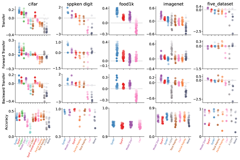
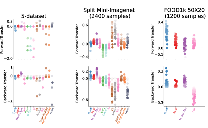
In this paper, We propose two lifelong learning algorithms, one based on ensembling decision forests (Syngeristic Forests, SynF), and another based on ensembling deep networks (Synergistic Networks, SynN). We explore our proposed algorithm as compared to a number of reference algorithms on an extensive suite of numerical experiments that span simulations, vision datasets including CIFAR-100, 5-dataset, Split Mini-Imagenet, and Food1k, as well as the spoken digit dataset. Figure 1 illustrates that our algorithms outperform all the reference algorithms in terms of forward, backward, and overall transfer in most of the cases. Ablation studies indicate the degree to which the amount of representation or storage capacity and replaying old task data impact performance of our algorithms. All our code and experiments are open source to facilitate reproducibility.
2 Mathematical Framework
2.1 The lifelong learning objective
Consider a lifelong learning environment with tasks, . We consider task aware lifelong learning, i.e., the tasks are known during both training and testing time. For simplicity, we consider that any task has the same input space, i.e., they have valued inputs with valued class labels. We assume the tasks arrive sequentially, but the data samples, within each task are batched and sampled identically and independently () from some fixed distribution. Here each sample within is the realization of random variable pair, and is the realization of distributed as the joint distribution . A learner trains on and chooses a hypothesis by minimizing a particular risk, where and are the algorithm and hypothesis space, respectively. In supervised learning settings, one can consider the following risk for a particular task :
| (1) |
where is a given loss function associated with the task and . Note that the data may contain data that is relevant to any number of tasks (potentially all the tasks) in the environment. One may take expectation with respect to for averaging out the randomness in the risk due to and consider the generalization error for the task as:
| (2) |
In the above equation, the learner will have access to a total of datasets after tasks, , instead of only. 111More generally, we may have datasets, where and each dataset may be associated with the target distributions of multiple tasks. For simplicity, we do not consider such scenarios further at this time. The goal is to find a learner that chooses a hypothesis such the generalization error over all the tasks after observing all the data is minimized, that is:
| (3) |
Note that can operate under any task , i.e., .
2.2 Lifelong learning evaluation criteria
Others have previously introduced criteria to evaluate transfer, including forward and backward transfer [23, 24, 25, 26]. Pearl [27] introduced the transfer benefit ratio, which builds directly off relative efficiency from classical statistics [28]. We define three notions of transfer building on relative efficiency.
Definition 1 (Transfer).
Overall transfer of algorithm for a given Task is:
| (4) |
We say that an algorithm has transferred to task from all the tasks up to if and only if .
Forward transfer quantifies how much performance a learner transfers forward to future tasks, given prior tasks.
Definition 2 (Forward Transfer).
The forward transfer of for task is :
| (5) |
We say an algorithm (positively) forward transfers for task if and only if .
Backwards transfer quantifies how much a learner transfers backward to previously observed tasks, in light of new tasks.
Definition 3 (Backward Transfer).
The backward transfer of for Task is:
| (6) |
We say an algorithm (positively) backward transfers to Task from all the tasks if and only if
.
Note that can be decomposed into and :
| (7) | ||||
| (8) |
Another paper, Veniat et al. [26], concomitantly introduced transfer and forgetting (backward transfer). Their statistics are the same as ours, except they do not use a . We opted for a to address numerical stability issues in comparing small numbers. Because log is a monotonic function, the order of ranking algorithms is preserved (Appendix Figure 1 shows a version of Figure 1 but using Veniat’s statistics, which is nearly visually identical). By virtue of introducing here, we can identify the inherent trade-off between forward and backward transfer, for a fixed amount of total transfer. Apart from the above statistics, we also report accuracy per task.
Definition 4 (Accuracy).
The accuracy of on task is after observing total datasets is:
| (9) |
3 Representation ensembling algorithms

Shannon proposed that a learner can be decomposed into three components: an encoder, a channel, and a decoder [29, 30]: . Figure 2 shows these three components as the building blocks of different learning schemas. The encoder, , maps an -valued input into an internal representation space [31, 32]. The channel maps the transformed data into a posterior distribution (or, more generally, a score). Finally, a decoder , produces a predicted label.
A canonical example of a single learner depicted in Figure 2A is a decision tree. Importantly, one can subsample the training data to learn different components of the tree [33, 34, 35]. For example, one can use a portion of data to learn the tree structure (which is the encoder). Then, by pushing the remaining data (sometimes called the ‘out-of-bag’ data) through the tree, one can learn posteriors in each leaf node (which are the channel). The channel thus gives scores for each data point denoting the probability of that data point belonging to a specific class. Using separate sets of data to learn the encoder and the channel results in less bias in the estimated posterior in the channels as in ‘honest trees’ [33, 34, 35]. Finally, the decoder provides the predicted class label using over the posteriors from the channel.
One can generalize the above decomposition by allowing for multiple encoders, as shown in Figure 2B. Given different encoders, one can attach a single channel to each encoder, yielding different channels. Doing so requires generalizing the definition of a decoder so that it would operate on multiple channels. Such a decoder ensembles the decisions, because here each channel provides the final output based on the encoder. This is the learning paradigm behind bagging [36] and boosting [37]; indeed, decision forests are a canonical example of a decision function operating on an ensemble of outputs [38].
Although the task specific structure in Figure 2B can provide useful decision on the corresponding task, they cannot, in general, provide meaningful decisions on other tasks, because those tasks might have completely different class labels. Therefore, in the multi-head structure (Figure 2C) a single encoder is used to learn a joint representation from all the tasks, and a separate channel is learned for each task to get the score or class conditional posteriors for each task, which is followed by each task specific decider [10, 13, 11].
Modular approaches, such as ProgNN and LMC (Figure 2D), have both multiple encoders and decoders. Connections from past to future encoders enables forward transfer. However, they freeze backward transfer.
Our approach also uses multiple encoders and decoders (Figure 2E). Unlike modular approaches, we allow connections across encoders to other channels, including both forwards and backwards. The result is that the channels ensemble representations (learned by the encoders), rather than decisions (learned by the channels). In our algorithms, we push all the data through each encoder, and each channel learns and ensembles across all encoders. When each encoder has learned complementary representations, the channels can leverage that information to improve over single task performance. This approach has applications, particularly in few-shot [39] and multiple task scenarios, including lifelong learning.
3.1 Our representation ensembling algorithms
We have developed two different representation ensembling algorithms based on bagging which are trained on different tasks. We draw analogy from the synergy of multiple independent representations on a particular task and call our algorithm ‘synergistic’. In both algorithms, as data from a new task arrives, the algorithm first builds a new independent encoder. Then, it builds the channel for this new task by pushing the new task data through all existing encoders. Thus the channel integrates information across all existing encoders using the new task data, thereby enabling forward transfer. At the same time, if it stores old task data (or can generate such data), it can push that data through the new encoders to update the channels from the old tasks, thereby enabling backward transfer. In either case, new test data are passed through all existing encoders and corresponding channels to make a prediction (see Appendix C for detailed description of this approach).
3.1.1 Synergistic Networks
A Synergistic Network (SynN) ensembles deep networks. For each task, the encoder in SynN is the “backbone” of a deep network (DN). Thus, each maps an element of to an element of , where is the number of neurons in the ultimate layer of the DN. The channels are learned via -Nearest Neighbors (-NN) [40] over the dimensional representations of . Recall that a -NN, with chosen such that as the number of samples goes to infinity, also goes to infinity, while , is a universally consistent classifier [40]. We use , which satisfies these conditions. The decoder outputs the argmax to produce a single prediction.
3.1.2 Synergistic Forests
Synergistic Forests (SynF) ensemble decision trees or forests. For each task, the encoder of SynF is the representation learned by a decision forest [41, 38]. The leaf nodes of each decision forest partition the input space into polytopes [33]. The channel then learns the class-conditional posteriors by populating the polytopes with out-of-task samples, as in “honest trees” [33, 34, 35]. Each channel outputs the posteriors averaged across the collection of forests learned over different tasks. The decoder outputs the argmax to produce a single prediction.
Note that the amount of additional representation capacity added per task by SynF is a function of the amount and complexity of the data for a new task. Contrast this with SynN and other deep net based modular or representation ensembling approaches, which a priori choose how much additional representation to add, prior to seeing all the new task data. So, SynF has capacity, space complexity, and time complexity scale with the complexity and sample size of each task. In contrast, ProgNN, SynN (and others like it) have a fixed capacity for each task, even if the tasks have very different sample sizes and complexities.
4 A computational taxonomy of lifelong learners
The space complexity of the learner refers to the amount of memory space needed to store the learner [42]. We also study the representation capacity of these algorithms. Capacity is defined as the size of the subset of hypotheses that is achievable by the learning algorithm [43].
We use the soft-O notation to quantify complexity [44]. Letting be the sample size and be the number of tasks, we write that the capacity, space or time complexity of a lifelong learning algorithm is when is bounded above asymptotically by a function of and up to a constant factor and polylogarithmic terms. For simplifying the calculation, we make the following assumptions:
-
1.
Each task has the same number of training samples.
-
2.
Capacity grows linearly with the number of trainable parameters in the model.
-
3.
The number of epochs is fixed for each task, independent of sample size.
-
4.
For the algorithms with dynamically expanding capacity, we assume the worst case scenario where an equal amount of capacity is added to the hypothesis with an additional task.
| Parametric | Capacity | Space | Time | Examples | ||
| () | () | () | ||||
| parametric | O-EWC, SI, LwF | |||||
| parametric | EWC | |||||
| parametric | Total Replay | |||||
| semi-parametric | ProgNN | |||||
| semi-parametric | DF-CNN | |||||
| semi-parametric | SynN, Model Zoo, DER, LMC | |||||
| non-parametric | SynF, IBP-WF | |||||
Assumption enables us to write time complexity as a function of the sample size. Table 1 summarizes the capacity, space and time complexity of several reference algorithms, as well as our SynN and SynF. For space and time complexity, the table shows results as a function of and , as well as the common scenario where sample size per task is fixed and therefore proportional to the number of tasks, . For detailed calculation of time complexity see Appendix E.
Parametric lifelong learning methods have a representational capacity which is invariant to sample size and task number. Although the space complexity of some of these algorithms grow (because the number of the constraints grows stored by the algorithms grows, or they continue to store more data), their capacity is fixed. Thus, given a sufficiently large number of tasks, in general, eventually all parametric methods will catastrophically forget. EWC [10], Online EWC [13], SI [11], and LwF [12] are all examples of parametric lifelong learning algorithms.
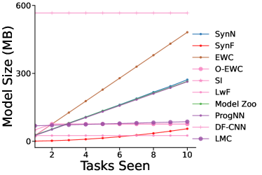
Semi-parametric algorithms’ representational capacity grows slower than sample size. For example, if is increasing slower than (e.g., ), then algorithms whose capacity is proportional to are semi-parametric. ProgNN [16] is semi-parametric, nonetheless, its space complexity due to the lateral connections. Moreover, the time complexity for ProgNN also scales quadratically with when . Thus, an algorithm that literally stores all the data it has ever seen, and retrains a fixed size network on all those data with the arrival of each new task, would have smaller space complexity and the same time complexity as ProgNN. For comparison, we implement such an algorithm and refer to it as Total Replay. DF-CNN [17] improves upon ProgNN by introducing a “knowledge base” with lateral connections to each new column, thereby avoiding all pairwise connections. Because these semi-parametric methods have a fixed representational capacity per task, they will either lack the representation capacity to perform well given sufficiently complex tasks, and/or will waste resources for very simple tasks. SynN and SynF eliminate the lateral connections between columns of the network, thereby reducing space complexity down to . Moreover, as shown in Figure 3, memory consumed by new channels is negligible compared to that of memory required for storing the encoders. Note that the time required for updating channels is negligible in comparison with the time required for training a new encoder.
Non-parametric algorithms’ representational capacity grows linearly with sample size. SynF is a non-parametric lifelong learning algorithm with its capacity, space and time complexity all , meaning that its representational capacity naturally increases with the complexity of each task. Apart from SynF, Indian Buffet Process for Weight Factors (IBP-WF) [45] proposed the only other non-parametric lifelong learning algorithm to our knowledge.
5 Providing intuition of synergistic learning through simulations
5.1 Forward and backward transfer in a simple environment
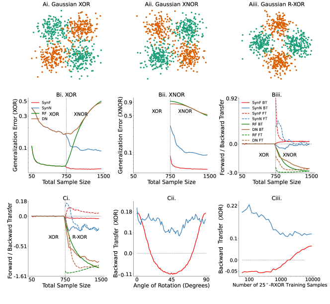
Consider a very simple two-task environment: Gaussian XOR and Gaussian Exclusive NOR (XNOR) (Figure 4A, see Appendix F for details). The two tasks share the exact same discriminant boundaries: the coordinate axes. Thus, transferring from one task to the other merely requires learning a bit flip of the class labels. We sample a total 750 samples from XOR, followed by another 750 samples from XNOR.
SynF and random forests (RF) achieve the same generalization error on XOR when training with XOR data (Figure 4Bi). But because RF does not account for a change in task, when XNOR data appear, RF performance on XOR deteriorates (it catastrophically forgets). In contrast, SynF continues to improve on XOR given XNOR data, demonstrating backward transfer. Now consider the generalization error on XNOR (Figure 4Bii). Both SynF and RF are at chance levels for XNOR when only XOR data are available. When XNOR data are available, RF must unlearn everything it learned from the XOR data, and thus its performance on XNOR starts out nearly maximally inaccurate, and quickly improves. On the other hand, because SynF can leverage the encoder learned using the XOR data, upon getting any XNOR data, it immediately performs quite well, and then continues to improve with further XNOR data, demonstrating forward transfer (Figure 4Biii). SynF demonstrates positive forward and backward transfer for all sample sizes, whereas RF fails to demonstrate forward or backward transfer, and eventually catastrophically forgets the previous tasks. Results for SynN and DN are qualitatively similar to those of SynF and RF respectively.
5.2 Forward and backward transfer for adversarial tasks
In the context of synergistic learning, we informally define a task to be adversarial with respect to task if the true joint distribution of task , without any domain adaptation, impedes performance on task . In other words, training data from task can only add noise, rather than signal, for task . An adversarial task for Gaussian XOR is Gaussian XOR rotated by (R-XOR) (Figure 4Aiii). Training on R-XOR therefore impedes the performance of SynF and SynN on XOR, and thus backward transfer becomes negative, demonstrating graceful forgetting [46] (Figure 4Ci). Because R-XOR is more difficult than XOR for SynF (because the discriminant boundaries are oblique [47]), and because the discriminant boundaries are learned imperfectly with finite data, data from XOR can actually improve performance on R-XOR, and thus forward transfer is positive. In contrast, both forward and backward transfer are negative for RF and DN.
To further investigate this relationship, we design a suite of R-XOR examples, generalizing R-XOR from only to any rotation angle between and , sampling 100 points from XOR, and another 100 from each R-XOR (Figure 4Cii). As the angle increases from to , flips from positive () to negative () for SynF. A similar trend is also visible for SynN. The -XOR is the maximally adversarial R-XOR. Thus, as the angle further increases, increases back up to at , which has an identical discriminant boundary to XOR. Moreover, when is fixed at , increases at different rates for different sample sizes of the source task (Figure 4Ciii).
Together, these experiments indicate that the amount of transfer can be a complicated function of (i) the difficulty of learning good representations for each task, (ii) the relationship between the two tasks, and (iii) the sample size of each. Appendix F further investigates this phenomenon in a multi-spiral environment.
6 Benchmark data experiments
For benchmark data, we build SynN encoders using the network architecture described in van de Ven et al. [48]. We use the same network architecture for all the benchmarking models. For the following experiments, we consider two modalities of real data: vision and language.
6.1 Reference algorithms
We compared our approaches to reference lifelong learning methods. Among them five are resource growing as well as modular approach: ProgNN [16], DF-CNN [17], LMC [49], Model Zoo[50], CoSCL [51]. Other reference algorithms are resource constrained: Elastic Weight Consolidation (EWC) [10], Online-EWC (O-EWC) [13], Synaptic Intelligence (SI) [11], Learning without Forgetting (LwF) [12], and “None”.
We also compare two variants of exact replay (Total Replay and Partial Replay) using the code provided by van de Ven et al. [48]. Both Total and Partial Replay store all the data they have ever seen, but Total Replay replays all of it upon acquiring a new task, whereas Partial Replay replays samples, randomly sampled from the entire corpus, whenever we acquire a new task with samples. Additionally, we have compared our approach with more constrained ways of replaying old task data, including Averaged Gradient Episodic Memory (A-GEM) [52], Experience Replay (ER) [53] and Task-based Accumulated Gradients (TAG) [54].
6.2 Exploring and explaining transfer capabilities via the CIFAR 10x10 dataset
The CIFAR 100 challenge [56], consists of 50,000 training and 10,000 test samples, each a 32x32 RGB image of a common object, from one of 100 possible classes, such as apples and bicycles. CIFAR 10x10 divides these data into 10 tasks, each with 10 classes [17] (see Appendix G for details).
6.2.1 Resource growing experiments
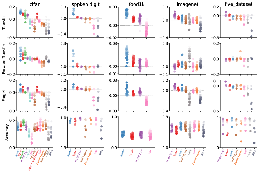
SynF, SynN, and Model Zoo demonstrate positive forward and backward transfer for every task in CIFAR 10x10, in contrast, other algorithms do not exhibit any positive backward transfer (Figure 1 first column). Moreover, they retained their accuracy while improving transfer (Figure 1, bottom row). ProgNN had a similar degree of forward transfer, but zero backward transfer, and requires quadratic space and time in sample size, unlike SynF, SynN, and Model Zoo which all require quasilinear space and time.
6.2.2 Ablation Experiments
Our proposed algorithms can improve performance on all the tasks (past and future) by both growing additional resources and replaying data from the past tasks. Below we do three ablation experiments using CIFAR 10X10 to measure the relative contribution of resource growth and replay on the performance of our proposed algorithms.
Resource constrained experiments
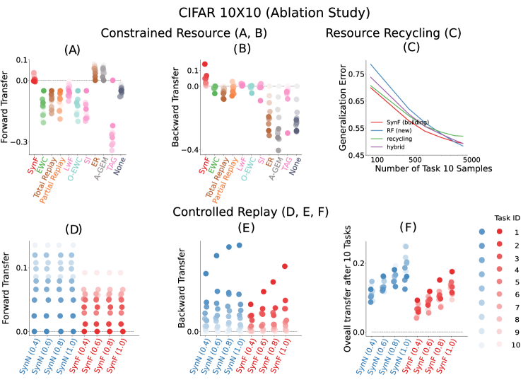
In this experiment, we devised a “resource constrained” variant of SynF experiments to observe the effect of ablating resource growth on SynF. In this constrained variant, we compare the lifelong learning algorithm to its single task variant, but ensure that they both have the same amount of resources. For example, on Task 2, we would compare SynF with 20 trees (10 trained on 500 samples from Task 1, and another 10 trained on 500 samples from Task 2) to RF with 20 trees (all trained on 500 samples Task 2). Although ablating the resource growth results in lower forward transfer compared to that of its resource growing variant (Figure 1 first column and Figure 5 top left), forward transfer remains positive after enough tasks, and backward transfer is actually invariant to this change (Figure 5, top left and center). In contrast, all of the reference algorithms that have fixed resources exhibit negative forward and backward transfer. Note that in this experiment, building the single task learners actually requires substantially more resources, specifically, trees, as compared with only trees in the prior experiments. In general, to ensure single task learners use the same amount of resources per task as our synergistic learners requires resources, where as SynF only requires .
Resource Recycling Experiments
The binary distinction we made above, algorithms either build resources or reallocate them, is a false dichotomy, and biologically unnatural. In biological learning, systems develop from building to fixed resources, as they grow from juveniles to adults. To explore this continuum of amount of resources to grow, we trained SynF on the first nine CIFAR 10x10 tasks using 50 trees per task, with 500 samples per task. For the tenth task, we could (i) select the 50 trees (out of the 450 existing trees) that perform best on task 10 (recycling), (ii) train 50 new trees, as SynF would normally do (building), (iii) build 25 and recruit 25 trees (hybrid), or (iv) ignore all prior trees (RF). SynF outperforms other approaches except when 5,000 training samples are available, but the recycling approach is nearly as good as SynF (Figure 5, top right). This result motivates future work to investigate optimal strategies for determining how to optimally leverage existing resources without growing new ones given a new task.
Controlled Replay Experiment
In this experiment, we train different versions of SynN and SynF sequentially on the tasks from CIFAR 10X10. The only difference between different versions of the algorithms is the amount of old task data replayed. In different versions of each algorithm, we replay , , and of the old task data respectively. As apparent from Figure 5 bottom, replaying old task data has no effect on forward transfer, but replaying more data improves backward transfer as the number of tasks increases.
6.2.3 Adversarial experiments
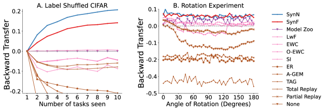
Consider the same CIFAR 10x10 experiments above, but, for Tasks 2 through 9, randomly permute the class labels within each task, rendering each of those tasks adversarial with regard to the first task (because the labels are uninformative). Figure 6A indicates that backward transfer for both SynF and SynN show positive backward transfer even with such label shuffling (the other algorithms did not demonstrate positive backward transfer). Now, consider a Rotated CIFAR experiment, which uses only data from the first task, divided into two equally sized subsets (making two tasks), where the second subset is rotated by different amounts (Figure 6, right). Backward transfer of both SynF and SynN is nearly invariant to rotation angle, whereas the other approaches are far more sensitive to rotation angle. Note that zero rotation angle corresponds to the two tasks having identical distributions. The fact that other algorithms fail to transfer even in this setting suggests that they may not ever be able to positively backwards transfer. See Appendix G.2 for additional experiment using CIFAR 10X10.
6.3 Further investigating transfer in additional datasets with more classes, tasks, and/or samples
6.3.1 Spoken Digit
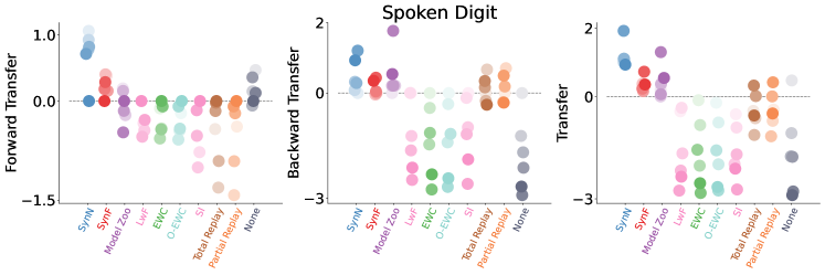
In this experiment, we used the Spoken Digit dataset [57]. As shown in Figure 1 second column, both SynF and SynN show positive backward and forward transfer between the spoken digit tasks, in contrast to other methods, some of which show only forward transfer, others show only backward transfer, with none showing both, and some showing neither. See Appendix G.3 for details of the experiment.
6.3.2 FOOD1k 50X20 Dataset
In this experiment, we use Food1k which is a large scale vision dataset consisting of food categories from Food2k [58]. FOOD1k 50X20 splits these data into tasks with classes each. For each class, we randomly sampled samples per class for training the models and used rest of the data for testing purpose. Because on the CIFAR experiments Model Zoo performs the best among the reference resource growing models, and LwF is the best performing resource constrained algorithm, we only use them as the reference models for the large scale experiment to avoid heavy computational cost. As shown in Figure 1 third column, SynN performs the best among all the algorithms on this large dataset.
6.3.3 Split Mini-Imagenet
In this experiment, we have used the Mini-Imagenet dataset [54]. The dataset was split into tasks with classes each. Each task has training samples and testing samples. As shown in Figure 1 fourth column, we get positive forward and backward transfer for both SynN and SynF. However, although samples per task is lower compared to that of 5-dataset, it is still quite high. Hence, Model Zoo outperforms all the algorithms in this experiment.
6.3.4 5-dataset
In this experiment, we have used 5-dataset [54]. It consists of tasks from five different datasets: CIFAR-10 [56], MNIST, SVHN [59], notMNIST [60], Fashion-MNIST [61]. All the monochromatic images were converted to RGB format, and then resized to . As shown in Appendix Table 4, training samples per task in -dataset is relatively higher than that of low data regime typically considered in lifelong learning setting. However, as shown in Figure 1 fifth column, SynN and SynF show less forgetting than most of the reference algorithms. On the other hand, Model Zoo shows comparatively better performance in relatively high task data size setup. Recall that SynN and SynF are based on bagging, and Model Zoo is based on boosting. It is well known that boosting often outperforms bagging when sample sizes are large 222Wyner et al. [62] shows that both bagging and boosting asymptotically converge to the Bayes optimal solution. However, for finite sample size and similar model complexity, we empirically find bagging approach to lifelong learning performs better than that of boosting when the training sample size is low whereas boosting performs better on large training sample size (See Figure 1). This is consistent with similar results in single task learning [63, 64, 25]. In lifelong learning, we are often primarily concerned with situations in which we have a small number of samples per task.
7 Discussion
We introduced quasilinear representation ensembling as an approach to synergistic lifelong learning. Two specific algorithms, SynF and SynN, achieve both forward and backward transfer, by leveraging resources (encoders) learned for other tasks without undue computational burdens. In this paper, we have mainly focused on task-aware setting, because it is simpler. Future work will extend our approach to more challenging task-unaware settings. Ablation experiments with CIFAR 10x10 shows that Forest-based representation ensembling approaches can easily add new resources when appropriate. This work therefore motivates additional research on deep learning to enable dynamically adding resources when appropriate, and resuse the older representations like the moduler methods [65, 66, 26, 49].
Acknowledgements
The authors thank the support of the NSF-Simons Research Collaborations on the Mathematical and Scientific Foundations of Deep Learning (NSF grant 2031985). We also thank Raman Arora, Dinesh Jayaraman, Rene Vidal, Jeremias Sulam, Guillermo Sapiro, and Michael Powell for helpful discussions. This work is graciously supported by the Defense Advanced Research Projects Agency (DARPA) Lifelong Learning Machines program through contracts FA8650-18-2-7834 and HR0011-18-2-0025. Research was partially supported by funding from Microsoft Research and the Kavli Neuroscience Discovery Institute.
References
- Mitchell [1999] Tom M Mitchell. Machine learning and data mining. Communications of the ACM, 42(11):30–36, 1999.
- Vapnik and Chervonenkis [1971] V Vapnik and A Chervonenkis. On the Uniform Convergence of Relative Frequencies of Events to Their Probabilities. Theory Probab. Appl., 16(2):264–280, January 1971.
- Valiant [1984] L G Valiant. A Theory of the Learnable. Commun. ACM, 27(11):1134–1142, November 1984. URL http://doi.acm.org/10.1145/1968.1972.
- Caruana [1997] Rich Caruana. Multitask learning. Machine learning, 28(1):41–75, 1997.
- Thrun [1996] Sebastian Thrun. Is learning the n-th thing any easier than learning the first? In Advances in neural information processing systems, pages 640–646, 1996.
- Thrun and Pratt [2012] Sebastian Thrun and Lorien Pratt. Learning to Learn. Springer Science & Business Media, December 2012. URL https://market.android.com/details?id=book-X_jpBwAAQBAJ.
- McCloskey and Cohen [1989] Michael McCloskey and Neal J Cohen. Catastrophic interference in connectionist networks: The sequential learning problem. In Psychology of learning and motivation, volume 24, pages 109–165. Elsevier, 1989.
- McClelland et al. [1995] James L McClelland, Bruce L McNaughton, and Randall C O’Reilly. Why there are complementary learning systems in the hippocampus and neocortex: insights from the successes and failures of connectionist models of learning and memory. Psychological review, 102(3):419, 1995.
- Zhao et al. [2016] Jing Zhao, Blanca Quiroz, L Quentin Dixon, and R Malatesha Joshi. Comparing Bilingual to Monolingual Learners on English Spelling: A Meta-analytic Review. Dyslexia, 22(3):193–213, August 2016.
- Kirkpatrick et al. [2017] James Kirkpatrick, Razvan Pascanu, Neil Rabinowitz, Joel Veness, Guillaume Desjardins, Andrei A Rusu, Kieran Milan, John Quan, Tiago Ramalho, Agnieszka Grabska-Barwinska, Demis Hassabis, Claudia Clopath, Dharshan Kumaran, and Raia Hadsell. Overcoming catastrophic forgetting in neural networks. Proceedings of the national academy of sciences, 114(13):3521–3526, 2017.
- Zenke et al. [2017] Friedemann Zenke, Ben Poole, and Surya Ganguli. Continual learning through synaptic intelligence. In Proceedings of the 34th International Conference on Machine Learning-Volume 70, pages 3987–3995. JMLR. org, 2017.
- Li and Hoiem [2017] Zhizhong Li and Derek Hoiem. Learning without forgetting. IEEE transactions on pattern analysis and machine intelligence, 40(12):2935–2947, 2017.
- Schwarz et al. [2018] Jonathan Schwarz, Jelena Luketina, Wojciech M Czarnecki, Agnieszka Grabska-Barwinska, Yee Whye Teh, Razvan Pascanu, and Raia Hadsell. Progress & compress: A scalable framework for continual learning. arXiv preprint arXiv:1805.06370, 2018.
- Finn et al. [2019] Chelsea Finn, Aravind Rajeswaran, Sham Kakade, and Sergey Levine. Online meta-learning. In Kamalika Chaudhuri and Ruslan Salakhutdinov, editors, International Conference on Machine Learning, volume 97 of Proceedings of Machine Learning Research, pages 1920–1930, Long Beach, California, USA, 06 2019. PMLR. URL http://proceedings.mlr.press/v97/finn19a.html.
- Ruvolo and Eaton [2013] Paul Ruvolo and Eric Eaton. ELLA: An Efficient Lifelong Learning Algorithm. In International Conference on Machine Learning, volume 28, pages 507–515, February 2013. URL http://proceedings.mlr.press/v28/ruvolo13.html.
- Rusu et al. [2016] Andrei A Rusu, Neil C Rabinowitz, Guillaume Desjardins, Hubert Soyer, James Kirkpatrick, Koray Kavukcuoglu, Razvan Pascanu, and Raia Hadsell. Progressive neural networks. arXiv preprint arXiv:1606.04671, 2016.
- Lee et al. [2019] Seungwon Lee, James Stokes, and Eric Eaton. Learning shared knowledge for deep lifelong learning using deconvolutional networks. In Proceedings of the 28th International Joint Conference on Artificial Intelligence, pages 2837–2844, 2019.
- Sodhani et al. [2020] Shagun Sodhani, Sarath Chandar, and Yoshua Bengio. Toward training recurrent neural networks for lifelong learning. Neural computation, 32(1):1–35, 2020.
- Parisi et al. [2019] German I Parisi, Ronald Kemker, Jose L Part, Christopher Kanan, and Stefan Wermter. Continual lifelong learning with neural networks: A review. Neural Networks, 2019.
- Chen and Liu [2016] Zhiyuan Chen and Bing Liu. Lifelong Machine Learning. Synthesis Lectures on Artificial Intelligence and Machine Learning, 10(3):1–145, November 2016. URL https://doi.org/10.2200/S00737ED1V01Y201610AIM033.
- Pearl [2019] Judea Pearl. The seven tools of causal inference, with reflections on machine learning. Commun. ACM, February 2019.
- Marcus and Davis [2019] Gary Marcus and Ernest Davis. Rebooting AI: Building Artificial Intelligence We Can Trust. Pantheon, September 2019.
- Lopez-Paz and Ranzato [2017] David Lopez-Paz and Marc’Aurelio Ranzato. Gradient episodic memory for continual learning. In NIPS, 2017.
- Benavides-Prado et al. [2018] Diana Benavides-Prado, Yun Sing Koh, and Patricia Riddle. Measuring Cumulative Gain of Knowledgeable Lifelong Learners. In NeurIPS Continual Learning Workshop, pages 1–8, 2018.
- Díaz-Rodríguez et al. [2018] Natalia Díaz-Rodríguez, Vincenzo Lomonaco, David Filliat, and Davide Maltoni. Don’t forget, there is more than forgetting: new metrics for continual learning. arXiv preprint arXiv:1810.13166, 2018.
- Veniat et al. [2020] Tom Veniat, Ludovic Denoyer, and Marc’Aurelio Ranzato. Efficient continual learning with modular networks and task-driven priors. arXiv preprint arXiv:2012.12631, 2020.
- Judea [2018] Pearl Judea. What is gained from past learning. Journal of Causal Inference, 6(1), 2018.
- Bickel and Doksum [2015] Peter J Bickel and Kjell A Doksum. Mathematical statistics: basic ideas and selected topics, volumes I-II package. Chapman and Hall/CRC, 2015.
- Cover and Thomas [2012] Thomas M Cover and Joy A Thomas. Elements of Information Theory. John Wiley & Sons, New York, November 2012.
- Cho et al. [2014] Kyunghyun Cho, B van Merrienboer, Caglar Gulcehre, F Bougares, H Schwenk, and Yoshua Bengio. Learning phrase representations using rnn encoder-decoder for statistical machine translation. In Conference on Empirical Methods in Natural Language Processing (EMNLP 2014), 2014.
- Vaswani et al. [2017] Ashish Vaswani, Noam Shazeer, Niki Parmar, Jakob Uszkoreit, Llion Jones, Aidan N Gomez, Ł Ukasz Kaiser, and Illia Polosukhin. Attention is All you Need. In I Guyon, U V Luxburg, S Bengio, H Wallach, R Fergus, S Vishwanathan, and R Garnett, editors, Advances in Neural Information Processing Systems 30, pages 5998–6008. Curran Associates, Inc., 2017.
- Devlin et al. [2018] Jacob Devlin, Ming-Wei Chang, Kenton Lee, and Kristina Toutanova. BERT: pre-training of deep bidirectional transformers for language understanding. CoRR, abs/1810.04805, 2018. URL http://arxiv.org/abs/1810.04805.
- Breiman et al. [1984] Leo Breiman, Jerome Friedman, Charles J Stone, and Richard A Olshen. Classification and regression trees. CRC press, 1984.
- Denil et al. [2014] M. Denil, D. Matheson, and N. De Freitas. Narrowing the gap: Random forests in theory and in practice. In Eric P. Xing and Tony Jebara, editors, Proceedings of the 31st International Conference on Machine Learning, volume 32 of Proceedings of Machine Learning Research, pages 665–673, 6 2014.
- Athey et al. [2019] S. Athey, J. Tibshirani, and S. Wager. Generalized random forests. Annals of Statistics, 47(2):1148–1178, 2019.
- Breiman [1996] Leo Breiman. Bagging predictors. Mach. Learn., 24(2):123–140, August 1996.
- Freund [1995] Y Freund. Boosting a Weak Learning Algorithm by Majority. Inform. and Comput., 121(2):256–285, September 1995.
- Breiman [2001] Leo Breiman. Random forests. Machine learning, 45(1):5–32, 2001.
- Dvornik et al. [2020] Nikita Dvornik, Cordelia Schmid, and Julien Mairal. Selecting relevant features from a multi-domain representation for few-shot classification. In Computer Vision–ECCV 2020: 16th European Conference, Glasgow, UK, August 23–28, 2020, Proceedings, Part X 16, pages 769–786. Springer, 2020.
- Stone [1977] Charles J Stone. Consistent Nonparametric Regression. Ann. Stat., 5(4):595–620, July 1977.
- Amit and Geman [1997] Yali Amit and Donald Geman. Shape Quantization and Recognition with Randomized Trees. Neural Comput., 9(7):1545–1588, October 1997.
- Kuo and Zuo [2003] Way Kuo and Ming J Zuo. Optimal reliability modeling: principles and applications. John Wiley & Sons, 2003.
- Zhang et al. [2021] Chiyuan Zhang, Samy Bengio, Moritz Hardt, Benjamin Recht, and Oriol Vinyals. Understanding deep learning (still) requires rethinking generalization. Communications of the ACM, 64(3):107–115, 2021.
- van Rooij et al. [2019] Iris van Rooij, Mark Blokpoel, Johan Kwisthout, and Todd Wareham. Cognition and Intractability: A Guide to Classical and Parameterized Complexity Analysis. Cambridge University Press, April 2019.
- Mehta et al. [2021] Nikhil Mehta, Kevin Liang, Vinay Kumar Verma, and Lawrence Carin. Continual learning using a bayesian nonparametric dictionary of weight factors. In International Conference on Artificial Intelligence and Statistics, pages 100–108. PMLR, 2021.
- Aljundi et al. [2018] Rahaf Aljundi, Francesca Babiloni, Mohamed Elhoseiny, Marcus Rohrbach, and Tinne Tuytelaars. Memory aware synapses: Learning what (not) to forget. In Vittorio Ferrari, Martial Hebert, Cristian Sminchisescu, and Yair Weiss, editors, Computer Vision – ECCV 2018, pages 144–161, Cham, 2018. Springer International Publishing.
- Tomita et al. [2020] Tyler M Tomita, James Browne, Cencheng Shen, Jaewon Chung, Jesse L Patsolic, Benjamin Falk, Jason Yim, Carey E Priebe, Randal Burns, Mauro Maggioni, and Joshua T Vogelstein. Sparse Projection Oblique Randomer Forests. J. Mach. Learn. Res., 2020.
- van de Ven et al. [2020] Gido M van de Ven, Hava T Siegelmann, and Andreas S Tolias. Brain-inspired replay for continual learning with artificial neural networks. Nature communications, 11:4069, 2020.
- Ostapenko et al. [2021] Oleksiy Ostapenko, Pau Rodriguez, Massimo Caccia, and Laurent Charlin. Continual learning via local module composition. Advances in Neural Information Processing Systems, 34:30298–30312, 2021.
- Ramesh and Chaudhari [2021] Rahul Ramesh and Pratik Chaudhari. Model zoo: A growing brain that learns continually. In International Conference on Learning Representations, 2021.
- Wang et al. [2022] Liyuan Wang, Xingxing Zhang, Qian Li, Jun Zhu, and Yi Zhong. Coscl: Cooperation of small continual learners is stronger than a big one. In European Conference on Computer Vision, pages 254–271. Springer, 2022.
- Chaudhry et al. [2018] Arslan Chaudhry, Marc’Aurelio Ranzato, Marcus Rohrbach, and Mohamed Elhoseiny. Efficient lifelong learning with a-gem. arXiv preprint arXiv:1812.00420, 2018.
- Chaudhry et al. [2019] Arslan Chaudhry, Marcus Rohrbach, Mohamed Elhoseiny, Thalaiyasingam Ajanthan, Puneet K Dokania, Philip HS Torr, and Marc’Aurelio Ranzato. On tiny episodic memories in continual learning. arXiv preprint arXiv:1902.10486, 2019.
- Malviya et al. [2021] Pranshu Malviya, Sarath Chandar, and Balaraman Ravindran. Tag: Task-based accumulated gradients for lifelong learning. arXiv preprint arXiv:2105.05155, 2021.
- van de Ven and Tolias [2019] Gido M. van de Ven and Andreas S. Tolias. Three scenarios for continual learning. CoRR, abs/1904.07734, 2019. URL http://arxiv.org/abs/1904.07734.
- Krizhevsky [2012] Alex Krizhevsky. Learning multiple layers of features from tiny images. University of Toronto, 05 2012.
- Jackson et al. [2018] Zohar Jackson, César Souza, Jason Flaks, Yuxin Pan, Hereman Nicolas, and Adhish Thite. Jakobovski/free-spoken-digit-dataset: v1. 0.8. Zenodo, August, 2018.
- Min et al. [2021] Weiqing Min, Zhiling Wang, Yuxin Liu, Mengjiang Luo, Liping Kang, Xiaoming Wei, Xiaolin Wei, and Shuqiang Jiang. Large scale visual food recognition. CoRR, abs/2103.16107, 2021.
- Netzer et al. [2011] Yuval Netzer, Tao Wang, Adam Coates, Alessandro Bissacco, Bo Wu, and Andrew Y Ng. Reading digits in natural images with unsupervised feature learning. 2011.
- Bulatov [2011] Yaroslav Bulatov. http://yaroslavvb.blogspot.com/2011/09/notmnist-dataset.html. 2011.
- Xiao et al. [2017] Han Xiao, Kashif Rasul, and Roland Vollgraf. Fashion-mnist: a novel image dataset for benchmarking machine learning algorithms. arXiv preprint arXiv:1708.07747, 2017.
- Wyner et al. [2017] Abraham J Wyner, Matthew Olson, Justin Bleich, and David Mease. Explaining the success of adaboost and random forests as interpolating classifiers. The Journal of Machine Learning Research, 18(1):1558–1590, 2017.
- Caruana and Niculescu-Mizil [2006] Rich Caruana and Alexandru Niculescu-Mizil. An Empirical Comparison of Supervised Learning Algorithms. In Proceedings of the 23rd International Conference on Machine Learning, ICML ’06, pages 161–168, New York, NY, USA, 2006. ACM.
- Caruana et al. [2004] Rich Caruana, Alexandru Niculescu-Mizil, Geoff Crew, and Alex Ksikes. Ensemble selection from libraries of models. In Proceedings of the twenty-first international conference on Machine learning, page 18, 2004.
- Yoon et al. [2017] Jaehong Yoon, Eunho Yang, Jeongtae Lee, and Sung Ju Hwang. Lifelong Learning with Dynamically Expandable Networks. International Conference on Learning Representations, August 2017.
- Mallya and Lazebnik [2018] Arun Mallya and Svetlana Lazebnik. Packnet: Adding multiple tasks to a single network by iterative pruning. In Proceedings of the IEEE conference on Computer Vision and Pattern Recognition, pages 7765–7773, 2018.
- Chen and Guestrin [2016] Tianqi Chen and Carlos Guestrin. XGBoost: A Scalable Tree Boosting System. In Proceedings of the 22nd ACM SIGKDD International Conference on Knowledge Discovery and Data Mining, KDD ’16, pages 785–794, New York, NY, USA, August 2016. Association for Computing Machinery.
- Qiu et al. [2014] Xueheng Qiu, Le Zhang, Ye Ren, Ponnuthurai N Suganthan, and Gehan Amaratunga. Ensemble deep learning for regression and time series forecasting. In 2014 IEEE symposium on computational intelligence in ensemble learning (CIEL), pages 1–6. IEEE, 2014.
- Potes et al. [2016] Cristhian Potes, Saman Parvaneh, Asif Rahman, and Bryan Conroy. Ensemble of feature-based and deep learning-based classifiers for detection of abnormal heart sounds. In 2016 computing in cardiology conference (CinC), pages 621–624. IEEE, 2016.
- Wang et al. [2003] Haixun Wang, Wei Fan, Philip S Yu, and Jiawei Han. Mining concept-drifting data streams using ensemble classifiers. In Proceedings of the ninth ACM SIGKDD international conference on Knowledge discovery and data mining, pages 226–235, 2003.
- Dai et al. [2007] Wenyuan Dai, Qiang Yang, Gui-Rong Xue, and Yong Yu. Boosting for transfer learning.(2007), 193–200. In Proceedings of the 24th international conference on Machine learning, 2007.
- Polikar et al. [2001] Robi Polikar, Lalita Upda, Satish S Upda, and Vasant Honavar. Learn++: An incremental learning algorithm for supervised neural networks. IEEE transactions on systems, man, and cybernetics, part C (applications and reviews), 31(4):497–508, 2001.
- van de Ven et al. [2022] Gido M van de Ven, Tinne Tuytelaars, and Andreas S Tolias. Three types of incremental learning. Nature Machine Intelligence, pages 1–13, 2022.
- Yan et al. [2021] Shipeng Yan, Jiangwei Xie, and Xuming He. Der: Dynamically expandable representation for class incremental learning. In Proceedings of the IEEE/CVF Conference on Computer Vision and Pattern Recognition, pages 3014–3023, 2021.
- Robins [1995] Anthony Robins. Catastrophic forgetting, rehearsal and pseudorehearsal. Connection Science, 7(2):123–146, 1995.
- Shin et al. [2017] Hanul Shin, Jung Kwon Lee, Jaehong Kim, and Jiwon Kim. Continual learning with deep generative replay. In Advances in Neural Information Processing Systems, pages 2990–2999, 2017.
- Caruana et al. [2008] Rich Caruana, Nikos Karampatziakis, and Ainur Yessenalina. An empirical evaluation of supervised learning in high dimensions. In Proceedings of the 25th international conference on Machine learning, pages 96–103, New York, New York, USA, July 2008. ACM.
- Fernández-Delgado et al. [2014] Manuel Fernández-Delgado, Eva Cernadas, Senén Barro, and Dinani Amorim. Do we need hundreds of classifiers to solve real world classification problems. J. Mach. Learn. Res., 15(1):3133–3181, 2014.
- Mehta et al. [2019] Ronak Mehta, Richard Guo, Cencheng Shen, and Joshua Vogelstein. Estimating information-theoretic quantities with random forests. arXiv preprint arXiv:1907.00325, 2019.
Appendix A Literature review
Prior work illustrates that ensembling learners can yield huge advantages in a wide range of applications. For example, in classical machine learning, ensembling trees leads to state-of-the-art random forest [38] and gradient boosting tree algorithms [67]. Similarly, ensembling networks shows promising results in various real-world applications [68, 69]. Wang et al. [70] used weighted ensemble of learners in a streaming setting with distribution shift. TrAdaBoost [71] boosts ensemble of learners to enable transfer learning. In continual learning scenarios, many algorithms have been built on these ideas by ensembling dependent representations. For example, Learn++ [72] boosts ensembles of weak learners learned over different data sequences in class incremental lifelong learning settings [73]. Model Zoo [50] uses the same boosting approach in task incremental lifelong learning scenarios.
Another group of algorithms, ProgNN [16] and DF-CNN [17] learn a new “column” of nodes and edges with each new task, and ensembles the columns for inference (such approaches are commonly called ‘modular’ now). The primary difference between ProgNN and DF-CNN is that ProgNN has forward connections to the current column from all the past columns. This creates the possibility of forward transfer while freezing backward transfer. However, the forward connections in ProgNN render it computationally inefficient for a large number of tasks. DF-CNN gets around this problem by learning a common knowledge base and thereby, creating the possibility of backward transfer.
Recently, many other modular approaches have been proposed in the literature that improve on ProgNN’s capacity growth. These methods consider the capacity for each task being composed of modules that can be shared across tasks and grown as necessary. For example, PackNet [66] starts with a fixed capacity network and trains for additional tasks by freeing up portion of the network capacity using iterative pruning. Veniat et al. [26] trains additional modules with each new task, and the old modules are only used selectively. Ostapenko et al. [49] improved the memory efficiency of the modular methods by adding new modules according to the complexity of the new tasks. Mehta et al. [45] proposed non-parametric factorization of the layer weights that promotes sharing of the weights between tasks. However, all of modular methods described above lack backward transfer because the old modules are not updated with the new tasks. Dynamically Expandable Representation (DER) [74] proposed an improvement over the modular approaches where the model capacity is dynamically expanded and the model is fine-tuned by replaying a portion of the old task data along with the new task data. This approach achieves backward transfer between tasks as reported by the authors in the experiments.
Another strategy for building lifelong learning machines is to use total or partial replay [48, 75, 76]. Replay approaches keep the old data and replay them when faced with new tasks to mitigate catastrophic forgetting. However, as we will illustrate, previously proposed replay algorithms do not demonstrate positive backward transfer in our experiments, though they often do not forget as much as other approaches.
Our approach builds directly on previously proposed modular and replay approaches with one key distinction: in our approach, representations are learned independently. Empirically, for low sample sizes random forests (which learn independent trees) typically outperform gradient boosted trees (which learn dependent trees) [64, 77, 78]. Because our approach of representation ensembling is similar to that of random forest, we expect learning independent representations to outperform learning dependent representations in these scenarios as well. This phenomenon is empirically shown in the main text Figure 1. Independent representations also have computational advantages, as doing so merely requires quasilinear time and space, and can be learned in parallel.
Appendix B Evaluation Criteria
Appendix C Representation Ensembling Algorithms
In this paper, we have proposed two representation ensembling algorithms, Synergistic Forests (SynF) and Synergistic Networks (SynN). The two algorithms differ in their details of how to update encoders and channels, but abstracting a level up they are both special cases of the same procedure. Let SynX refer to any possible synergistic algorithm. Algorithms 1, 2, 3, and 4 provide pseudocode for adding encoders, updating channels, and making predictions for any SynX algorithm. Whenever the learner gets access to a new task data, we use Algorithm 1 to train a new encoder for the corresponding task. We split the data into two portions — one set is used to learn the encoder and the other portion is called the held out or out-of-bag (OOB) data which is returned by Algorithm 1 to be used by Algorithm 2 to learn the channel for the corresponding task. Note that we push the OOB data through the in-task encoder and the whole dataset through the cross-task encoders to update the channel, i.e, learn the posteriors according to the new encoder. Then we use Algorithm 3 to replay the old task data through the new encoder and update their corresponding channels. Finally, while predicting for a test sample, we use Algorithm 4. Given the task identity, we use the corresponding channel to get the average estimated posterior and predict the class label as the of the estimated posteriors.
| Hyperparameters | Value |
|---|---|
| n_estimators ( training samples per task) | |
| n_estimators ( training samples per task) | |
| max_depth | |
| max_samples (OOB split) | |
| min_samples_leaf |
| Hyperparameters | Value |
|---|---|
| n_estimators | |
| max_depth | |
| max_samples (OOB split) | |
| min_samples_leaf |
| Hyperparameters | Value |
|---|---|
| optimizer | Adam |
| learning rate | |
| max_samples (OOB split) | |
| K (KNN channel) |
Appendix D Reference Algorithm Implementation Details
The same network architecture was used for all compared deep learning methods. Following van de Ven et al. [48], the ‘base network architecture’ consisted of five convolutional layers followed by two-fully connected layers each containing 2000 nodes with ReLU non-linearities and a softmax output layer. The convolutional layers had , , , and channels, they used batch-norm and a ReLU non-linearity, they had a 3x3 kernel, a padding of 1 and a stride of 2 (except the first layer, which had a stride of 1). This architecture was used with a multi-headed output layer (i.e., a different output layer for each task) for all algorithms using a fixed-size network. For ProgNN and DF-CNN the same architecture was used for each column introduced for each new task, and in our SynN this architecture was used for the transformers (see above). In these implementations, ProgNN and DF-CNN have the same architecture for each column introduced for each task. Among the reference algorithms, EWC, O-EWC, LwF, SI, Total Replay and Partial Replay results were produced using the repository https://github.com/GMvandeVen/progressive-learning-pytorch. For ProgNN and DF-CNN we used the code provided in https://github.com/Lifelong-ML/DF-CNN. For all other reference algorithms, we modified the code provided by the authors to match the deep net architecture as mentioned above and used the default hyperparameters provided in the code.
Appendix E Training Time Complexity Analysis
Consider a lifelong learning environment with tasks each with samples, i.e., total training samples, . For all the algorithm with time complexity , the training time grows linearly with more training samples. We discuss all other algorithms with non-linear time complexity below.
E.1 EWC
Consider the time required to train the weights for each task in EWC is and each task adds additional time from the regularization term. Here, and are both constants. Therefore, time required to learn all the tasks can be written as:
| (10) |
E.2 Total Replay
Consider the time to train the model on samples is . Therefore, time required to learn all the tasks can be written as:
| (11) |
E.3 ProgNN
Consider the time required to train each column in ProgNN is and each lateral connection can be learned with time . Therefore, time required to learn all the tasks can be written as:
| (12) |
Appendix F Simulated Results
In each simulation, we constructed an environment with two tasks. For each, we sample 750 times from the first task, followed by 750 times from the second task. These 1,500 samples comprise the training data. We sample another 1,000 hold out samples to evaluate the algorithms. We fit a random forest (RF) (technically, an uncertainty forest which is an honest forest with a finite-sample correction [79]) and a SynF. For SynN, we have used a deep network (DN) architecture with two hidden layers each having nodes. Similarly, for SynN experiments we did repetitions and reported the results after smoothing it using moving average with a window size of . For the SynF experiments we used repetitions and reported the mean of these repetitions. We repeat this process 30 times to obtain errorbars. Error bars in all cases were negligible.
F.1 Gaussian XOR
Gaussian XOR is two class classification problem with equal class priors. Conditioned on being in class 0, a sample is drawn from a mixture of two Gaussians with means , and variances proportional to the identity matrix. Conditioned on being in class 1, a sample is drawn from a mixture of two Gaussians with means , and variances proportional to the identity matrix. Gaussian XNOR is the same distribution as Gaussian XOR with the class labels flipped. Rotated XOR (R-XOR) rotates XOR by degrees.
F.2 Spirals
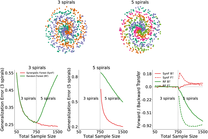
A description of the distributions for the two tasks is as follows: let be the number of classes and multinomial. Conditioned on , each feature vector is parameterized by two variables, the radius and an angle . For each sample, is sampled uniformly in . Conditioned on a particular class, the angles are evenly spaced between and where controls the number of turns in the spiral. To inject noise along the spiral, we add Gaussian noise to the evenly spaced angles . The observed feature vector is then . In Figure 2 we set , , and .
Consider an environment with a three spiral and five spiral task (Figure 2). In this environment, axis-aligned splits are inefficient, because the optimal partitions are better approximated by irregular polytopes than by the orthotopes provided by axis-aligned splits. The three spiral data helps the five spiral performance because the optimal partitioning for these two tasks is relatively similar to one another, as indicated by positive forward transfer. This is despite the fact that the five spiral task requires more fine partitioning than the three spiral task. Because SynF grows relatively deep trees, it over-partitions space, thereby rendering tasks with more coarse optimal decision boundaries useful for tasks with more fine optimal decision boundaries. The five spiral data also improves the three spiral performance.
Appendix G Real Data Extended Results
FOOD1k and Mini-Imagenet datasets were obtained from https://www.kaggle.com/datasets/whitemoon/miniimagenet and https://github.com/pranshu28/TAG, respectively.
| Experiment | Dataset | Training samples | Testing samples | Dimension |
|---|---|---|---|---|
| CIFAR 10X10 | CIFAR 100 | |||
| 5-dataset | CIFAR-10 | (resized) | ||
| MNIST | ||||
| SVHN | ||||
| notMNSIT | ||||
| Fashion-MNIST | ||||
| Split Mini-Imagenet | Mini-Imagenet | |||
| FOOD1k 50X20 | Food1k | (resized) | ||
| Spoken Digit | Spoken Digit | (processed and resized) |
| Algorithms | |
|---|---|
| SynN | |
| SynF | |
| Model Zoo | |
| ProgNN | |
| LMC | |
| CoSCL | |
| DF-CNN | |
| EWC | |
| Total Replay | |
| Partial Replay | |
| SynF(resource constrained) | |
| LwF | |
| O-EWC | |
| SI | |
| ER | |
| A-GEM | |
| TAG | |
| None |
| Algorithms | |
|---|---|
| SynN | |
| SynF | |
| Model Zoo | |
| EWC | |
| Total Replay | |
| Partial Replay | |
| LwF | |
| O-EWC | |
| SI | |
| ER | |
| A-GEM | |
| TAG | |
| None |
| Algorithms | |
|---|---|
| SynN | |
| SynF | |
| Model Zoo | |
| EWC | |
| Total Replay | |
| Partial Replay | |
| LwF | |
| O-EWC | |
| SI | |
| ER | |
| A-GEM | |
| TAG | |
| None |
| Algorithms | |
|---|---|
| SynN | |
| SynF | |
| Model Zoo | |
| LwF |
| Hyperparameters | Value |
|---|---|
| n_estimators ( training samples per task) | |
| max_depth | |
| max_samples (OOB split) | |
| min_samples_leaf |
G.1 CIFAR 10x10
| Task # | Image Classes |
|---|---|
| 1 | apple, aquarium fish, baby, bear, beaver, bed, bee, beetle, bicycle, bottle |
| 2 | bowl, boy, bridge, bus, butterfly, camel, can, castle, caterpillar |
| 3 | chair, chimpanzee, clock, cloud, cockroach, couch, crab, crocodile, cup, dinosaur |
| 4 | dolphin, elephant, flatfish, forest, fox, girl, hamster, house, kangaroo, keyboard |
| 5 | lamp, lawn mower, leopard, lion, lizard, lobster, man, maple tree, motor cycle, mountain |
| 6 | mouse, mushroom, oak tree, orange, orchid, otter, palm tree, pear, pickup truck, pine tree |
| 7 | plain, plate, poppy, porcupine, possum, rabbit, raccoon, ray, road, rocket |
| 8 | rose, sea, seal, shark, shrew, skunk, skyscraper, snail, snke, spider |
| 9 | squirrel, streetcar, sunflower, sweet pepper, table, tank, telephone, television, tiger, tractor |
| 10 | train, trout, tulip, turtle, wardrobe, whale, willow tree, wolf, woman, worm |
G.2 CIFAR 10x10 Repeated Classes
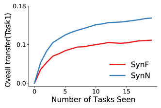
We also considered the setting where each task is defined by a random sampling of 10 out of 100 classes with replacement. This environment is designed to demonstrate the effect of tasks with shared subtasks, which is a common property of real world lifelong learning tasks. Supplementary Figure 3 shows transfer of SynF and SynN on Task 1.
Supplementary Table 10 shows the image classes associated with each task number.
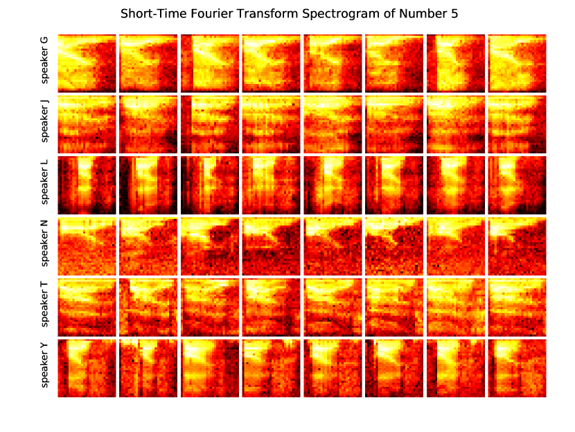
G.3 Spoken Digit experiment
In this experiment, we used the Spoken Digit dataset provided in https://github.com/Jakobovski/free-spoken-digit-dataset. The dataset contains audio recordings from six different speakers with recordings for each digit per speaker ( recordings in total). The experiment was set up with six tasks where each task contains recordings from only one speaker. For each recording, a spectrogram was extracted using Hanning windows of duration ms with an overlap of ms between the adjacent windows. The spectrograms were resized down to . The extracted spectrograms from eight random recordings of ‘’ for six speakers are shown in Figure 5. For each Monte Carlo repetition of the experiment, spectrograms extracted for each task were randomly divided into train and test set. The experiment is summarized in Figure 6. Note that we could not run the experiment on other reference algorithms using the code provided by their authors.
