Towards causal generative scene models
via competition of experts
Abstract
Learning how to model complex scenes in a modular way with recombinable components is a pre-requisite for higher-order reasoning and acting in the physical world. However, current generative models lack the ability to capture the inherently compositional and layered nature of visual scenes. While recent work has made progress towards unsupervised learning of object-based scene representations, most models still maintain a global representation space (i.e., objects are not explicitly separated), and cannot generate scenes with novel object arrangement and depth ordering. Here, we present an alternative approach which uses an inductive bias encouraging modularity by training an ensemble of generative models (experts). During training, experts compete for explaining parts of a scene, and thus specialise on different object classes, with objects being identified as parts that re-occur across multiple scenes. Our model allows for controllable sampling of individual objects and recombination of experts in physically plausible ways. In contrast to other methods, depth layering and occlusion are handled correctly, moving this approach closer to a causal generative scene model. Experiments on simple toy data qualitatively demonstrate the conceptual advantages of the proposed approach.
1 Introduction
Proposed in the early days of computer vision Grenander (1976); Horn (1977), analysis-by-synthesis is an approach to the problem of visual scene understanding. The idea is conceptually elegant and appealing: build a system that is able to synthesize complex scenes (e.g., by rendering), and then understand analysis (inference) as the inverse of this process that decomposes new scenes into their constituent components. The main challenges in this approach are the need for generative models of objects (and their composition into scenes) and the need to perform tractable inference given new inputs, including the task to decompose scenes into objects in the first place. In this work, we aim to learn such as system in an unsupervised way from observations of scenes alone.
A

B


C

While models such as vaes (Kingma & Welling, 2014; Rezende et al., 2014) and gans (Goodfellow et al., 2014) constitute significant progress in generative modelling, these models still lack the ability to capture the compositional nature of reality: they typically generate entire images or scenes at once, i.e., with a single pass through a large feedforward network. While this approach works well for objects such as centred faces—and progress has been impressive on those tasks Karras et al. (2019a; b)—generating natural scenes containing several objects in non-trivial constellations gets increasingly difficult within this framework due to the combinatorial number of compositions that need to be represented and reasoned about (Bau et al., 2019).
Image formation entangles different components in highly non-linear ways, such as occlusion. Due to the difficulty of choosing the correct model and the complexity of inference, the task to generate complex scenes containing compositions of objects still lacks success stories. More training data certainly helps, and progress on generating visually impressive scenes has been substantial Radford et al. (2015), but we hypothesize that a satisfactory and robust solution that is not optimized to a relatively well constrained IID (independent and identically distributed) data scenario will require that our models correctly incorporate the (causal) generative nature of natural scenes.
Here, we take some first small steps towards addressing the aforementioned limitations by proposing econ, a more physically-plausible generative scene model with explicitly compositional structure. Our approach is based on two main ideas. The first is to consider scenes as layered compositions of (partially) depth-ordered objects. The second is to represent object classes separately using an ensemble of generative models, or experts.
Our generative scene model consists of a sequential process which places independent objects in the scene, operating from the back to the front, so that objects occurring closer to the viewer can occlude those further away. During inference, this process is reversed: at each step, experts compete for explaining part of the remaining scene, and only the winning expert is further trained on the explained part (Parascandolo et al., 2018). This competition ideally drives each expert to specialise on representing and generating instances from one, or a few related, object classes or concepts, and the notion of “objects” should automatically emerge as contiguous regions that appear in a stable way across a range of training images. By decomposing scenes in the reverse order of generation, occluded objects can be inpainted within the already explained regions so that experts can learn to generate full, unoccluded objects which can be recombined in novel ways.
Learning a modular scene representation via object-specific experts has several benefits. First, each expert only needs to solve the simpler subtask of representing and generating instances from a single object class—something which current generative models have been shown to be capable of—while the composition process is treated separately. Secondly, expert models are useful in their own right as they can be dropped or added, reused and repurposed for other tasks on an individual level.
We highlight the following contributions.
- •
-
•
In section 4, we present econ, a compositional scene model, which, for a single expert, can be seen as extension of monet (Burgess et al., 2019) into a proper generative model (section 5.1).
-
•
We introduce modular object representations through separate generators and propose a competition mechanism and objective to drive experts to specialise in section 5.2.
-
•
In experiments on synthetic data in section 6 we show qualitatively that econ is able to decompose simple scenes into objects, represent these separately, and recombine them in a layer-wise fashion into novel, coherent scenes with arbitrary numbers and depth-orderings of objects.
-
•
We critically discuss our assumptions and propose extensions for future work in section 7.
2 The layer-based model of visual scenes
To reflect the fact that 2D images are the result of projections of richer 3D scenes, we assume that data are generated from the well-known dead leaves model,111the name derives from the analogy of leaves falling onto a canvas, covering whatever is beneath them, i.e., in a layer-wise fashion, see Figure 2(a) for an illustration. Starting with an empty canvas , an image is sequentially generated in steps. At each step we sample an object from one of different classes and place it on the canvas as follows,
| for | ||||
| object class | ||||
| object properties | ||||
| shape | ||||
| appearance | ||||
| place on canvas |
where represents the object class drawn at step ; is an abstract representation of the object’s properties; is a binary image determining shape; is a full (unmasked) image containing the object; and denotes element-wise multiplication. The corresponding graphical model is shown in Figure 2(b).222W.l.o.g., we assume that the background corresponds to with , see Figure 2(a).
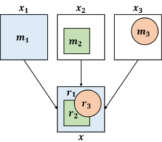
This sequential generation process captures the loss of depth information when projecting from 3D to 2D and is a natural way of handling occlusion phenomena. Consequently, sampling from this model is straightforward. We therefore consider it a more truthful approach to modelling visual scenes than, e.g., spatial mixture models, in line with Le Roux et al. (2011).
On the other hand, inferring the objects composing a given image is challenging. We will distinguish between shapes and regions in the following sense. The unoccluded object shapes , top row in Figure 2(a), remain hidden and only appear in via their corresponding, partially occluded segmentation regions , see the final composition in the bottom row of Figure 2(a) for an illustration. In particular, a region is always subset of the corresponding shape pixels .
In addition to the separate treatment of shapes and regions , we also introduce a scope variable to help write the above model in a convenient form. Following Burgess et al. (2019), is defined recursively as
| (1) |
The scope at time contains those parts of the image, which have been completely generated after steps and will not be occluded in the subsequent steps.
With , the regions can be compactly defined as
| (2) |
Using these, we can express the final composition as
| (3) |
While (3) may look like a normal spatial mixture model, it is worth noting the following important point: even though the shapes are drawn independently, the resulting segmentation regions become (temporally) dependent due to the layer-wise generation process, i.e., the visible part of object depends on all objects subsequently placed on the canvas. This seems very intuitive and is evident from the fact that the RHS of (2) is a function of .
3 Related work
Clustering & spatial mixture models
One line of work (Greff et al., 2016; 2017; Van Steenkiste et al., 2018) approaches the perceptual grouping task of decomposing scenes into components by viewing separate regions as clusters. A scene is modelled with a spatial mixture model, parametrised by deep neural networks, in which learning is performed with a procedure akin to expectation maximisation (EM; Dempster et al., 1977). The recent iodine model of Greff et al. (2019) instead uses a refinement network (Marino et al., 2018) to perform iterative amortised variational inference over independent scene components which are separately decoded and then combined via a softmax to form the scene. While iodine is able to decompose a given scene, it cannot generate coherent samples of new scenes because dependencies between regions due to layering are not explicitly captured in its generative model.
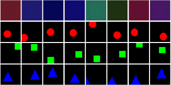
This shortcoming of iodine has also been pointed out by Engelcke et al. (2019) and addressed in their genesis model, which explicitly models dependencies between regions via an autoregressive prior over . While this does enable sampling of coherent scenes which look similar to training data, genesis still assumes an additive, rather than layered, model of scene composition. As a consequence, the resulting entangled component samples contain holes and partially occluded objects and cannot be easily layered and recombined as shown in Figure 1 (e.g., to generate samples with exactly two circles and one triangle).
Sequential models
Our work is closely related to sequential or recurrent approaches to image decomposition and generation (Mnih et al., 2014; Gregor et al., 2015; Eslami et al., 2016; Kosiorek et al., 2018; Yuan et al., 2019). In particular, we build on the recent monet model for scene decomposition of Burgess et al. (2019). monet combines a recurrent attention network with a VAE which encodes and reconstructs the input within the selected attention regions while unconstrained to inpaint occluded parts outside .
We extend this approach in two main directions. Firstly, we turn monet into a proper generative model333in its original form, it is a conditional model which does not admit a canonical way of sampling new scenes which respects the layer-wise generation of scenes described in section 2. Secondly, we explicitly model the discrete variable (object class) with an ensemble of class-specific VAEs (the experts)—as opposed to within a single large encoder-decoder architecture as in iodine, genesis or monet. Such specialisation allows to control object constellations in new, but scene-consistent ways.
Competition of experts
To achieve specialisation on different object classes in our model, we build on ideas from previous work using competitive training of experts (Jacobs & Jordan, 1991). More recently, these ideas have been successfully applied to tasks such as lifelong learning (Aljundi et al., 2017), learning independent causal mechanisms (Parascandolo et al., 2018), training mixtures of generative models (Locatello et al., 2018), as well as to dynamical systems via sparsely-interacting recurrent independent mechanisms (Goyal et al., 2019).
Probabilistic RBM models
The work of Le Roux et al. (2011) and Heess (2012) introduced probabilistic scene models that also reason about occlusion. Le Roux et al. (2011) combine restricted Boltzmann machines (rbms) to generate masks and shape separately for every object in the scenes into a masked rbm (m-rbm) model. Two variants are explored: one that respects a depth ordering and object occlusions, derived from similar arguments as we have put forward in the introduction; and a second model which uses a softmax combination akin to the spatial mixture models used in iodine and genesis, although the authors argue it makes little sense from a modelling perspective. Inference is implemented as blocked Gibbs sampling with contrastive divergence as a learning objective. Inference over depth ordering is done exhaustively, that is, considering every permutation—as opposed to greedily using competition as in this work. Shortcomings of the model are mainly the limited expressiveness of rbms (complexity and extent), as well as the cost of inference. Our work can be understood as an extension of the m-rbm formulation using VAEs in combination with attention, or segmentation, models.
| o X[6, m, l] X[1, m, c] X[1, m, c] X[1, m, c] X[1, m, c] X[1, m, c] | monet | iodine | genesis | m-rbm | econ |
|---|---|---|---|---|---|
| decompose scenes into objects and reconstruct | ✓ | ✓ | ✓ | ✓ | ✓ |
| generate coherent scenes like training data | ✗ | ✗ | ✓ | ✓ | ✓ |
| controllably recombine objects in novel ways | ✗ | ✗ | ✗ | ✓ | ✓ |
| efficient (amortised) inference | ✓ | ✓ | ✓ | ✗ | ✓ |
Vision as inverse graphics & probabilistic programs
Another way to programmatically introduce information about scene composition is through analysis-by-synthesis, see Bever & Poeppel (2010) for an overview. In this approach, the synthesis (i.e., generative) model is fully specified, e.g., through a graphics renderer, and inference becomes the inverse task, which poses a challenging optimisation problem. Probabilistic programming is often advocated as a means to automatically compile this inference task; for instance, picture has been proposed by Kulkarni et al. (2015), and combinations with deep learning have been explored by Wu et al. (2017). This approach is sometimes also understood as an instance of Approximate Bayesian Computation (ABC; Dempster et al., 1977) or likelihood-free inference. While conceptually appealing, these methods require a detailed specification of the scene generation process—something that we aim to learn in an unsupervised way. Furthermore, gains achieved by a more accurate scene generation process are generally paid for by complicated inference, and most methods thus rely on variations of MCMC sampling schemes (Jampani et al., 2015; Wu et al., 2017).
Supervised approaches
There is a body of work on augmenting generative models with ground-truth segmentation and other supervisory information. Turkoglu et al. (2019) proposed a layer based model to add objects onto a background, Ashual & Wolf (2019) proposed a scene-generation method allowing for fine grained user control, Karras et al. (2019a; b) have achieved impressive image generation results by exclusively training on a single class of objects. The key difference of these approaches to our work is that we exclusively focus on unsupervised approaches.
4 Ensemble of competing object nets (econ)
We now introduce econ (for Ensemble of Competing Object Networks), a causal generative scene model which explicitly captures the compositional nature of visual scenes. On a high level, the proposed architecture is an ensemble of generative models, or experts, designed after the layer-based scene model described in section 2. During training, experts compete to sequentially explain a given scene via attention over image regions, thereby specialising on different object classes. We perform variational inference (Jordan et al., 1999), amortised within the popular VAE framework (Kingma & Welling, 2014; Rezende et al., 2014), and use competition to greedily maximise a lower bound to the conditional likelihood w.r.t. object identity.
4.1 Generative model
We adopt the generative model described in section 2, parametrise it by , and assume that it factorises over the graphical model in Figure 2(b) (i.e., assuming that objects at different time steps are drawn independently of each other). We model with a categorical distribution,444though we will generally condition on , see section 5 for details, and place a unit-variance isotropic Gaussian prior over ,
Next, we parametrise and using decoders with respective parameters .555 is a hyperparameter (– 1 object classes and background) which has to be chosen domain dependently. These compute object means and mask probabilities which determine pixel-wise distributions over and via
| (4) | ||||
| (5) |
where and is a constant variance.
We note at this point that, while other handlings of the discrete variable are possible, we deliberately opt for separate decoders: (i) as an inductive bias encouraging modularity; and (ii) to be able to controllably sample individual objects and recombine them in novel ways.
Finally, we need to specify a distribution over . Due to its layer-wise generation, this is tricky and most easily done in terms of the visible regions . From (3), (5), and linearity of Gaussians it follows that, pixel-wise,
| (6) |
Similarly, one can show from (1), (2), and (4) that depends on only via , and that
| (7) |
for ; see Appendix A for detailed derivations.
The class-conditional joint distribution then factorises as,
| (8) |
Conditioning on is motivated by our inference procedure, see section 5. Moreover, we express in terms of the segmentation regions as only these are visible in the final composition which makes is easier to specify a distribution over . Note, however, that while we will perform inference over regions , we will learn to generate full shapes which are consistent with the inferred when composed layer-wise as captured in (7), thus respecting the physical data-generating process.
4.2 Approximate posterior
Since exact inference is intractable in our model, we approximate the posterior over and with the following variational distribution parametrised by and ,
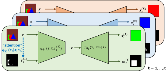
As for the generative distribution, we model dependence on using modules with separate parameters , …, . These inference modules consist of two parts.
Attention nets compute region probabilities and amortise inference over regions via
| (9) |
Encoders compute means and log-variances which parametrise distributions over via
We refer to the collection of , , and for a given as an expert as it implements all computations (generation and inference) for a specific object class—see Figure 3 for an illustration.
5 Inference
Due to the assumed sequential generative process, the natural order of inference is the reverse (), i.e., foreground objects should be explained first and the background last. This is also captured by the dependence of on via the scope in .
Such entanglement of scene components across composition steps makes inference over the entire scene intractable. We therefore choose the following greedy approach. At each inference step , we consider explanations from all possible object-classes —as provided by our ensemble of experts via attending, encoding and reconstructing different parts of the current scene—and then choose the best fitting one. This offers an intuitive foreground to background decomposition of an image as foreground objects should be easier to reconstruct.
Concretely, we first lower bound the marginal likelihood conditioned on , , and then use a competition mechanism between experts to determine the best . We now describe this inference procedure in more detail.
5.1 Objective: class-conditional ELBO
First, we lower bound the class-conditional model evidence using the approximate posterior as follows (see Appendix A for a detailed derivation):
Next, we use the reparametrization trick of Kingma & Welling (2014) to replace expectations w.r.t. by a Monte Carlo estimate using a single sample drawn as:
Finally, we approximate expectations w.r.t. in and using the Bernoulli means . We opt for directly using a continuous approximation and against sampling discrete ’s (e.g., using continuous relaxations to the Bernoulli distribution (Maddison et al., 2017; Jang et al., 2017)) as our generative model does not require the ability to directly sample regions. (Instead, we sample ’s and decode them into unoccluded shapes which can be combined layer-wise to form scenes.)
With these approximations, we obtain the estimates
| (10) | ||||
| (11) | ||||
| (12) |
which we combine to form the learning objective
| (13) |
where are hyperparameters. Note that for , (13) still approximates a valid lower bound.
Generative model extension of monet as a special case
For (i.e., ignoring different object classes for the moment), our derived objective (13) is similar to that used by Burgess et al. (2019). However, we note the following crucial difference in (12): in our model, reconstructed attention regions are multiplied by in the term of the KL, see (7). This implies that the generated shapes are constrained to match the attention region only within the current scope , so that—unlike in monet—the decoder is not penalised for generating entire unoccluded object shapes, allowing inpainting also on the level of masks. With just a single expert, our model can thus be understood as a generative model extension of monet.
5.2 Competition mechanism
For , i.e., when explicitly modelling object classes with separate experts, the objective (13) cannot be optimised directly because it is conditioned on the object identities . To address this issue, we use the following competition mechanism between experts.
At each inference step , we apply all experts to the current input and declare that expert the winner which yields the best competition objective (see below).666Applying all experts can be easily parallelised. We then use the winning expert to reconstruct the selected scene component using
where is encoded from the region attended by the winning expert . We then compute the contribution to (13) from step assuming fixed , and use it to update the winning expert with a gradient step. Finally, we update the scope using the winning expert,
| (14) |
to allow for inpainting within the explained region in the following inference (decomposition) steps.777To ensure that the entire scene is explained in steps, we use the final scope as attention region for all experts in the last inference step , as also done in genesis and monet.
This competition process can be seen as a greedy approximation to maximising (13) w.r.t. . While considering all possible object combinations would require steps, our competition procedure is linear in the number of object classes and runs in steps. By choosing an expert at each step , we approximate the expectation w.r.t. —which entangles the different composition steps and makes inference intractable—using and the updates in (14).
Competition objective
While model parameters are updated using the learning objective (13) derived from the ELBO, the choice of competition objective is ours. Since we use competition to drive specialisation of experts on different object classes and to greedily infer , (i.e., the identity of the current foreground object), the competition objective should reflect such differences between object classes. Object classes can differ in many ways (shape, color, size, etc) and to different extents, so the choice of competition objective is data-dependent and may be informed by prior knowledge.
For instance, in the setting depicted in Figure 1 where both color and shape are class-specific, we found that using a combination of and worked well. However, on the same data with randomised color (as used in the experiments in section 6) it did not: due to the greedy optimisation procedure, the expert which is initially best at reconstructing a particular color continues to win the competition for explaining regions of that color and thus receives gradient updates to reinforce this specialisation; such undesired specialisation corresponds to a local minimum in the optimisation landscape and can be very hard for the model to escape.
We thus found that relying solely on as the competition objective (i.e., the reconstruction of the attention region) helps to direct specialisation towards objects categories. In this case, experts are chosen based on how well they can model shape, and only those experts which can easily reconstruct (the shape of) a selected region within the current scope will do well at any given step, meaning that the selected region corresponds to a foreground object.
Moreover, we found that using a stochastic, rather than deterministic form of competition, (i.e., experts win the competition with the probabilities proportional to their competition objectives at a given step) helped specialisation. In particular, such approach helps prevent the collapse of the experts in the initial stages of training.
Formally, the probability of expert winning the competition is
with and being the terms in (13) at step for an expert . The hyper-parameter controls the relative influence of the appearance and shape reconstruction objectives to make the data-dependent assumptions about the competition mechanism as discussed above.
6 Experimental results
To explore econ’s ability to decompose and generate new scenes, we conduct experiments on synthetic data consisting of colored 2D objects or sprites (triangles, squares and circles) in different occlusion arrangements. We refer to Appendix C for a detailed account of the used data set, model architecture, choice of hyperparameters, and experimental setting. Further experiments can be found in Appendix B.
econ decomposes scenes and inpaints occluded objects
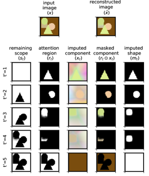
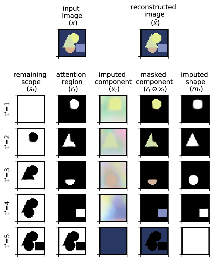
Fig. 4 shows an example of how econ decomposes a scene with four objects. At each inference step, the winning expert segments a region (second col.) within the unexplained part of the image (first col.), and reconstructs the selected object within the attended region (fourth col.). A distinctive feature of our model is that, despite occlusion, the full shape (rightmost col.) of every object is imputed (e.g., at step ). This ability to infer complete shapes is a consequence of the assumed layer-wise generative model which manifests itself in our objective via the unconstrained shape reconstruction term (12).
econ generalizes to novel scenes
Fig. 4 also illustrates that that the model is capable of decomposing scenes containing multiple objects of the same category, as well as multiple objects of the same color in separate steps. It does so for a scene with four objects, despite being trained on scenes containing only three objects, one from each class.

Single expert as generative extension of monet
We also investigate training a single expert which we claim to be akin to a generative extension of monet. When trained on the data from Fig. 1 with ground truth masks provided, the expert learns to inpaint occluded shapes and objects as can be seen from the samples in Fig. 5. However, all object classes are represented in a shared latent space so that different classes cannot be sampled controllably.


Multiple experts specialise on different object classes
Fig. 1B shows samples from each of the four experts trained on a dataset with uniquely colored objects (Fig. 1A). The samples from each expert contain either the same object in different spatial positions or differently coloured background, indicating that the experts specialised on the different object classes composing these scenes.
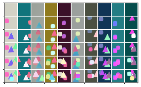
Fig. 6 shows the same plot for a model trained on scenes consisting of randomly colored objects. This setting is considerably more challenging because experts have to specialise purely based on shape while also representing color variations. Yet, experts specialise on different object classes: samples in Fig. 6 are either randomly colored background or objects from mostly one class with different colours and spatial positions, indicating that the econ is capable of representing the scenes as compositions of distinct objects in an unsupervised way.
Controlled and layered generation of new scenes
The specialisation of experts allows us to controllably generate new scenes with specific properties. To do so, we follow the sequential generation procedure described in section 2 by sampling from one of the experts at each time step. The number of generation steps , as well as the choices of experts allow to control the total number and categories of objects in the generated scene.
Fig. 1C shows samples generated using the experts in Fig. 1B. In Fig. 7 we show another example where more and more randomly colored objects are sequentially added. Even though the generated scenes are quite simple, we believe this result is important as the ability to generate scenes in a controlled way is a distinctive feature of our model, which current generative scene models lack.
7 Discussion
Model assumptions
While econ aims at modelling scene composition in a faithful way, we make a number of assumptions for the sake of tractable inference, which need to be revisited when moving to more general environments. We assume a known (maximum) number of object classes which may be restrictive for realistic settings, and choosing too small may force each expert to represent multiple object classes. Other assumptions are that the pixel values are modelled as normally distributed, even though they are discrete in the range , and that pixels are conditionally independent given shapes and objects.
Shared vs. object-specific representations
Recent work on unsupervised representation learning (Bengio et al., 2013) has largely focused on disentangling factors of variation within a single shared representation space, e.g., by training a large encoder-decoder architecture with different forms of regularization (Higgins et al., ; Kim & Mnih, 2018; Chen et al., 2018; Locatello et al., 2019). This is motivated by the observation that certain (continuous) attributes such as position, size, orientation or color are general concepts which transcend object-class boundaries. However, the range of values of these attributes, as well as other (discrete) properties such as shape, can strongly depend on object class. In this work, we investigate the other extreme of this spectrum by learning entirely object-specific representations. Exploring the more plausible middle ground combining both shared and object-specific representations is an attractive direction for further research.
Extensions and future work
The goal of decomposing visual scenes into their constituents in an unsupervised manner from images alone will likely remain a long standing goal of visual representation learning. We have presented a model that recombines earlier ideas on layered scene compositions, with more recent models of larger representational power, and unsupervised attention models. The focus of this work is to establish physically plausible compositional models for an easy class of images and to propose a model that naturally captures object-specific specialization.
With econ and other models as starting point, a number of extensions are possible. One direction of future work deals with incorporating additional information about scenes. Here, we consider static, semantically-free images. Optical flow and depth information can be cues to an attention process, facilitating segmentation and specialization. First results in the direction of video data have been shown by Xu et al. (2019). Natural images typically carry semantic meaning and objects are not ordered in arbitrary configurations. Capturing dependencies between objects (e.g., using an auto-regressive prior over depth ordering as in genesis), albeit challenging, could help disambiguate between scene components. Another direction of future work is to relax the unsupervised assumption, e.g., by exploring a semi-supervised approach, which might help improve stability.
On the modelling side, extensions to recurrent architectures and iterative refinement as in iodine appear promising. Our model entirely separates experts from each other but, depending on object similarity, one can also include shared representations which will help transfer already learned knowledge to new experts in a continual learning scenario.
8 Conclusion
While the scenes studied here and in the recent works of Burgess et al. (2019); Greff et al. (2019); Engelcke et al. (2019) are still in stark contrast to the impressive results that holistic generative models are able to achieve, we believe it is the right time to revisit the unsupervised scene composition problem. Our goal is to build re-combineable systems, where different components can be used for new scene inference tasks. In the spirit of the analysis-by-synthesis approach, this requires the ability to re-create physically plausible visual scenes. Disentangling the scene formation process from the objects is one crucial component thereof, and the vast number of object types will require the ability of unsupervised learning from visual input alone.
Acknowledgements
The authors would like to thank Alex Smola, Anirudh Goyal, Muhammad Waleed Gondal, Chris Russel, Adrian Weller, Neil Lawrence, and the Empirical Inference “deep learning & causality” team at the MPI for Intelligent Systems for helpful discussions and feedback.
M.B. and B.S. acknowledge support from the German Science Foundation (DFG) through the CRC 1233 “Robust Vision” project number 276693517, the German Federal Ministry of Education and Research (BMBF) through the Tübingen AI Center (FKZ: 01IS18039A), and the DFG Cluster of Excellence “Machine Learning – New Perspectives for Science” EXC 2064/1, project number 390727645.
References
- Aljundi et al. (2017) Rahaf Aljundi, Punarjay Chakravarty, and Tinne Tuytelaars. Expert gate: Lifelong learning with a network of experts. In Proceedings of the IEEE Conference on Computer Vision and Pattern Recognition, pp. 3366–3375, 2017.
- Ashual & Wolf (2019) Oron Ashual and Lior Wolf. Specifying object attributes and relations in interactive scene generation. In Proceedings of the IEEE International Conference on Computer Vision, pp. 4561–4569, 2019.
- Bau et al. (2019) David Bau, Jun-Yan Zhu, Jonas Wulff, William Peebles, Hendrik Strobelt, Bolei Zhou, and Antonio Torralba. Seeing what a gan cannot generate. In Proceedings of the IEEE International Conference on Computer Vision, pp. 4502–4511, 2019.
- Bengio et al. (2013) Yoshua Bengio, Aaron Courville, and Pascal Vincent. Representation learning: A review and new perspectives. IEEE transactions on pattern analysis and machine intelligence, 35(8):1798–1828, 2013.
- Bever & Poeppel (2010) Thomas G. Bever and David Poeppel. Analysis by synthesis: A (re-)emerging program of research for language and vision. Biolinguistics, 4(2):174–200, 2010.
- Burgess et al. (2019) Christopher P Burgess, Loic Matthey, Nicholas Watters, Rishabh Kabra, Irina Higgins, Matt Botvinick, and Alexander Lerchner. Monet: Unsupervised scene decomposition and representation. arXiv preprint arXiv:1901.11390, 2019.
- Chen et al. (2018) Tian Qi Chen, Xuechen Li, Roger B Grosse, and David K Duvenaud. Isolating sources of disentanglement in variational autoencoders. In Advances in Neural Information Processing Systems, pp. 2610–2620, 2018.
- Dempster et al. (1977) Arthur P Dempster, Nan M Laird, and Donald B Rubin. Maximum likelihood from incomplete data via the em algorithm. Journal of the Royal Statistical Society: Series B (Methodological), 39(1):1–22, 1977.
- Engelcke et al. (2019) Martin Engelcke, Adam R Kosiorek, Oiwi Parker Jones, and Ingmar Posner. Genesis: Generative scene inference and sampling with object-centric latent representations. arXiv preprint arXiv:1907.13052, 2019.
- Eslami et al. (2016) SM Ali Eslami, Nicolas Heess, Theophane Weber, Yuval Tassa, David Szepesvari, Geoffrey E Hinton, et al. Attend, infer, repeat: Fast scene understanding with generative models. In Advances in Neural Information Processing Systems, pp. 3225–3233, 2016.
- Goodfellow et al. (2014) Ian Goodfellow, Jean Pouget-Abadie, Mehdi Mirza, Bing Xu, David Warde-Farley, Sherjil Ozair, Aaron Courville, and Yoshua Bengio. Generative adversarial nets. In Advances in neural information processing systems, pp. 2672–2680, 2014.
- Goyal et al. (2019) Anirudh Goyal, Alex Lamb, Jordan Hoffmann, Shagun Sodhani, Sergey Levine, Yoshua Bengio, and Bernhard Schölkopf. Recurrent independent mechanisms. arXiv preprint arXiv:1909.10893, 2019.
- Greff et al. (2016) Klaus Greff, Antti Rasmus, Mathias Berglund, Tele Hao, Harri Valpola, and Jürgen Schmidhuber. Tagger: Deep unsupervised perceptual grouping. In Advances in Neural Information Processing Systems, pp. 4484–4492, 2016.
- Greff et al. (2017) Klaus Greff, Sjoerd Van Steenkiste, and Jürgen Schmidhuber. Neural expectation maximization. In Advances in Neural Information Processing Systems, pp. 6691–6701, 2017.
- Greff et al. (2019) Klaus Greff, Raphaël Lopez Kaufman, Rishabh Kabra, Nick Watters, Christopher Burgess, Daniel Zoran, Loic Matthey, Matthew Botvinick, and Alexander Lerchner. Multi-object representation learning with iterative variational inference. In International Conference on Machine Learning, pp. 2424–2433, 2019.
- Gregor et al. (2015) Karol Gregor, Ivo Danihelka, Alex Graves, Danilo Rezende, and Daan Wierstra. Draw: A recurrent neural network for image generation. In International Conference on Machine Learning, pp. 1462–1471, 2015.
- Grenander (1976) Ulf Grenander. Pattern synthesis – lectures in pattern theory. 1976.
- Heess (2012) Nicolas Manfred Otto Heess. Learning generative models of mid-level structure in natural images. PhD thesis, 2012.
- (19) Irina Higgins, Loic Matthey, Arka Pal, Christopher Burgess, Xavier Glorot, Matthew Botvinick, Shakir Mohamed, and Alexander Lerchner. beta-vae: Learning basic visual concepts with a constrained variational framework.
- Horn (1977) Berthold K. P. Horn. Understanding image intensities. Artifical Intelligence, 8:201–231, 1977.
- Jacobs & Jordan (1991) Robert A Jacobs and Michael I Jordan. A competitive modular connectionist architecture. In Advances in neural information processing systems, pp. 767–773, 1991.
- Jampani et al. (2015) Varun Jampani, Sebastian Nowozin, Matthew Loper, and Peter V. Gehler. The informed sampler: A discriminative approach to bayesian inference in generative computer vision models. Computer Vision and Image Understanding, 136:32 – 44, 2015. ISSN 1077-3142.
- Jang et al. (2017) Eric Jang, Shixiang Gu, and Ben Poole. Categorical reparametrization with gumbel-softmax. In International Conference on Learning Representations (ICLR 2017). OpenReview. net, 2017.
- Jordan et al. (1999) Michael I Jordan, Zoubin Ghahramani, Tommi S Jaakkola, and Lawrence K Saul. An introduction to variational methods for graphical models. Machine learning, 37(2):183–233, 1999.
- Karras et al. (2019a) Tero Karras, Samuli Laine, and Timo Aila. A style-based generator architecture for generative adversarial networks. In Proceedings of the IEEE Conference on Computer Vision and Pattern Recognition, pp. 4401–4410, 2019a.
- Karras et al. (2019b) Tero Karras, Samuli Laine, Miika Aittala, Janne Hellsten, Jaakko Lehtinen, and Timo Aila. Analyzing and improving the image quality of stylegan. arXiv preprint arXiv:1912.04958, 2019b.
- Kim & Mnih (2018) Hyunjik Kim and Andriy Mnih. Disentangling by factorising. arXiv preprint arXiv:1802.05983, 2018.
- Kingma & Ba (2014) Diederik P Kingma and Jimmy Ba. Adam: A method for stochastic optimization. arXiv preprint arXiv:1412.6980, 2014.
- Kingma & Welling (2014) Diederik P. Kingma and Max Welling. Auto-encoding variational bayes. In 2nd International Conference on Learning Representations, ICLR 2014, Banff, AB, Canada, April 14-16, 2014, Conference Track Proceedings, 2014.
- Kosiorek et al. (2018) Adam Kosiorek, Hyunjik Kim, Yee Whye Teh, and Ingmar Posner. Sequential attend, infer, repeat: Generative modelling of moving objects. In Advances in Neural Information Processing Systems, pp. 8606–8616, 2018.
- Kulkarni et al. (2015) T. D. Kulkarni, P. Kohli, J. B. Tenenbaum, and V. Mansinghka. Picture: A probabilistic programming language for scene perception. In IEEE Conference on Computer Vision and Pattern Recognition (CVPR), pp. 4390–4399, June 2015. doi: 10.1109/CVPR.2015.7299068.
- Le Roux et al. (2011) Nicolas Le Roux, Nicolas Heess, Jamie Shotton, and John Winn. Learning a generative model of images by factoring appearance and shape. Neural Computation, 23(3):593–650, 2011.
- Locatello et al. (2018) Francesco Locatello, Damien Vincent, Ilya Tolstikhin, Gunnar Rätsch, Sylvain Gelly, and Bernhard Schölkopf. Competitive training of mixtures of independent deep generative models. arXiv preprint arXiv:1804.11130, 2018.
- Locatello et al. (2019) Francesco Locatello, Stefan Bauer, Mario Lucic, Gunnar Raetsch, Sylvain Gelly, Bernhard Schölkopf, and Olivier Bachem. Challenging common assumptions in the unsupervised learning of disentangled representations. In International Conference on Machine Learning, pp. 4114–4124, 2019.
- Maddison et al. (2017) C Maddison, A Mnih, and Y Teh. The concrete distribution: A continuous relaxation of discrete random variables. International Conference on Learning Representations, 2017.
- Marino et al. (2018) Joe Marino, Yisong Yue, and Stephan Mandt. Iterative amortized inference. In International Conference on Machine Learning, pp. 3403–3412, 2018.
- Mnih et al. (2014) Volodymyr Mnih, Nicolas Heess, Alex Graves, et al. Recurrent models of visual attention. In Advances in neural information processing systems, pp. 2204–2212, 2014.
- Parascandolo et al. (2018) Giambattista Parascandolo, Niki Kilbertus, Mateo Rojas-Carulla, and Bernhard Schölkopf. Learning independent causal mechanisms. In International Conference on Machine Learning, pp. 4036–4044, 2018.
- Paszke et al. (2019) Adam Paszke, Sam Gross, Francisco Massa, Adam Lerer, James Bradbury, Gregory Chanan, Trevor Killeen, Zeming Lin, Natalia Gimelshein, Luca Antiga, Alban Desmaison, Andreas Kopf, Edward Yang, Zachary DeVito, Martin Raison, Alykhan Tejani, Sasank Chilamkurthy, Benoit Steiner, Lu Fang, Junjie Bai, and Soumith Chintala. Pytorch: An imperative style, high-performance deep learning library. In H. Wallach, H. Larochelle, A. Beygelzimer, F. dÁlché Buc, E. Fox, and R. Garnett (eds.), Advances in Neural Information Processing Systems 32, pp. 8024–8035. 2019.
- Radford et al. (2015) Alec Radford, Luke Metz, and Soumith Chintala. Unsupervised representation learning with deep convolutional generative adversarial networks. arXiv preprint arXiv:1511.06434, 2015.
- Rezende et al. (2014) Danilo Jimenez Rezende, Shakir Mohamed, and Daan Wierstra. Stochastic backpropagation and approximate inference in deep generative models. In International Conference on Machine Learning, pp. 1278–1286, 2014.
- Ronneberger et al. (2015) Olaf Ronneberger, Philipp Fischer, and Thomas Brox. U-net: Convolutional networks for biomedical image segmentation. In Nassir Navab, Joachim Hornegger, William M. Wells, and Alejandro F. Frangi (eds.), Medical Image Computing and Computer-Assisted Intervention – MICCAI 2015, pp. 234–241, Cham, 2015. Springer International Publishing. ISBN 978-3-319-24574-4.
- Turkoglu et al. (2019) Mehmet Ozgur Turkoglu, William Thong, Luuk Spreeuwers, and Berkay Kicanaoglu. A layer-based sequential framework for scene generation with gans. In Proceedings of the AAAI Conference on Artificial Intelligence, volume 33, pp. 8901–8908, 2019.
- Van Steenkiste et al. (2018) Sjoerd Van Steenkiste, Michael Chang, Klaus Greff, and Jürgen Schmidhuber. Relational neural expectation maximization: Unsupervised discovery of objects and their interactions. arXiv preprint arXiv:1802.10353, 2018.
- Wu et al. (2017) Jiajun Wu, Joshua B Tenenbaum, and Pushmeet Kohli. Neural scene de-rendering. In Proceedings of the IEEE Conference on Computer Vision and Pattern Recognition, pp. 699–707, 2017.
- Xu et al. (2019) Zhenjia Xu, Zhijian Liu, Chen Sun, Kevin Murphy, William T Freeman, Joshua B Tenenbaum, and Jiajun Wu. Unsupervised discovery of parts, structure, and dynamics. arXiv preprint arXiv:1903.05136, 2019.
- Yuan et al. (2019) Jinyang Yuan, Bin Li, and Xiangyang Xue. Generative modeling of infinite occluded objects for compositional scene representation. In International Conference on Machine Learning, pp. 7222–7231, 2019.
Appendix A Derivations
A.1 Derivation of ELBO
We now provide a detailed derivation of the evidence lower bound (ELBO) used in the main paper. For ease of notation we use vector notation and omit explicitly summing over pixel- and latent dimensions (as done in the implementation).
We start by writing as an expectation w.r.t. using importance sampling as follows:
Applying the concave function and using Jensen’s inequality we obtain
| (A.1) |
Using the chain rule of probability and properties of , we can rearrange the integrand on the RHS of (A.1) as
| (A.2) |
We will consider the three terms in (A.2) separately and define their expectations w.r.t. the approximate posterior as
Next, we use our modelling assumptions stated in the paper to simplify these terms, starting with .
Using the assumed factorisation of the approximate posterior, in particular , as well as the fact that , splitting the expectation into two parts, and using linearity of the expectation operator, we find that can be written as follows:
Next, we consider . Using a similar argument as for , we find that
Finally, we consider . Substituting the Gaussian likelihood for , ignoring constants which do not depend on any learnable parameters, and using the fact that is binary and , we obtain
where denotes the pixel-wise L2-norm between two RGB vectors. (Recall that , , and are defined as quantities in , , and , respectively, and that summation over these dimensions yields the desired scalar objective.)
We observe that , , and can all be written as sums over the composition steps.
We thus define:
Finally, it then follows that
A.2 Derivation of generative region distribution
We now derive the distribution in (7). We will use the fact that , and that can be written as , as well as the conditional independencies implied by our model, see Figure 2(b). Considering the pixel-wise distribution and marginalising over , we obtain:
Since is binary, this fully determines its distribution.
Appendix B Additional experimental results
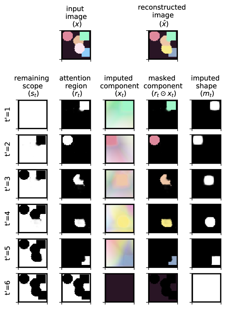
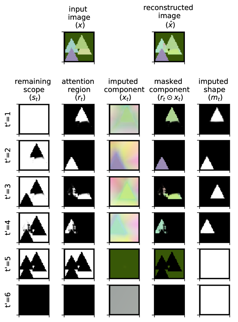
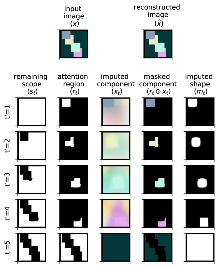
Figure 8 shows four additional examples of econ decomposing scenes consisting of multiple randomly coloured shapes. The model was trained on the data from Fig. 6, but is able to decompose scenes with five objects (a), multiple occluding objects from the same class (b, c), and objects of similar color to the background (d). Moreover, (b) suggests that additional timesteps () are simply ignored if they are not needed.
Appendix C Experimental details
C.1 Datasets
Synthetic dataset: uniquely colored objects
The dataset consists of images of circles, squares and triangles on a randomly and uniformly colored background, such that there is a unique correspondence between object color and class identites (red circles, green squares, blue triangles). The background color is randomly chosen to be an RGB value with each channel being a random integer between 0 and 127, while the RGB values of the object colors are (255,0,0), (0,255,0), (0,0,255) for circles, squares and triangles respectively. The spatial positions of the objects are randomly chosen such that each of the objects entirely fits into an image without crossing the image boundary.
The models shown in Fig. 1 and 5 have been trained on a version of such dataset containing images with exactly three objects per image (one of each class) in random depth orders (Fig. 1, top row). The training and validation splits include \num50000 and 100 such images respectively.
Synthetic dataset: randomly colored objects
This dataset is the same as the one described above with the difference that the objects (circles, squares and triangles) are randomly colored with the corresponding RGB values being random integers between 128 and 255.
The models shown in Fig. 4, 6 and 8 have been trained on a version of such dataset containing images with exactly three objects per image (one of each class) in random depth orders (Fig. 6, top row). The training and validation splits include 50000 and 100 such images respectively.
C.2 Architecture details
Each expert in our model consists of attention network computing the segmentation regions as a function of the input image and the scope at a given time step, and a VAE reconstructing the image appearance within the segmentation region and inpainting the unoccluded shape of object. Below we describe the details of architectures we used for each of the expert networks.
C.2.1 Expert VAEs
Encoder
The VAE encoder consists of multiple blocks, each of which is composed of convolutional layer, ReLU non-linearity, and max pooling. The output of the final block is flattened and transformed into a latent space vector by means of two fully connected layers. The output of the first fully-connected layer has 4 times the number of latent dimensions activations, which are passed through the ReLU activation, and finally linearly mapped to the latent vector by a second fully-connected layer.
Decoder
Following Burgess et al. (2019), we use spatial a broadcast decoder. First, the latent vector is repeated on a spatial grid of the size of an input image, resulting in a 3D tensor with spatial dimensions being that of an input, and as many feature maps as there are dimensions in the latent space. Second, we concatenate the two coordinate grids (for and coordinates) to this tensor. Next, this tensor is processed by a decoding network consisting of as many blocks as the encoder, with each block including a convolutional layer and ReLU non-linearity. Finally, we apply a convolutional layer with sigmoid activation to the output of the decoding network resulting in an output of 4 channel (RGB + shape reconstruction).
C.2.2 Attention network
We use the same attention network architecture as in Burgess et al. (2019) and the implementation provided by Engelcke et al. (2019). It consists of U-Net (Ronneberger et al., 2015) with 4 down and up blocks consisting of a convolutional layer, instance normalisation, ReLU activation and down- or up-sampling by a factor of two. The numbers of channels of the block outputs in the down part (the up part is symmetric) of the network are: 4 - 32 - 64 - 64 - 64.
C.3 Training details
We implemented the model in PyTorch (Paszke et al., 2019). We use the batch size of 32, Adam optimiser (Kingma & Ba, 2014), and initial learning rate of . We compute the validation loss every 100 iterations, and if the validation loss doesn’t improve for 5 consecutive evaluations, we decrease the learning rate by a factor of . We stop the training after 5 learning rate decrease step.
C.4 Cross-validation
Synthetic dataset: uniquely colored objects
The results in Fig. 1 were obtained by cross-validating 512 randomly sampled architectures with the following ranges of parameters:
| Parameter | Range |
|---|---|
| Latent dimension | 2 to 3 |
| Number of layers in encoder and decoder | 2 to 4 |
| Number of features per layer in encoder and decoder | 4 to 32 |
| (KL term weight in (12)) | 0.5 to 2 |
| (shape reconstruction weight in (12)) | 0.1 to 10 |
| Number of experts | 4 (three objects + background) |
| Number of time steps | 4 (three objects + background) |
The best performing model in terms of the validation loss (which is shown in Fig. 1) has the latent dimension of 2, 4 layers in encoder and decoder, 32 features per layer, and .
The results in Fig. 5 were obtained using the same model as above but with one expert.
Synthetic dataset: randomly colored objects
The results in Figs. 4, 6, and 7 were obtained by cross-validating 512 randomly sampled architectures with the following ranges of parameters:
| Parameter | Range |
|---|---|
| Latent dimension | 4 to 5 |
| Number of layers in encoder and decoder | 3 to 4 |
| Number of features per layer in encoder and decoder | 16 to 32 |
| (KL term weight in (12)) | 1 |
| (shape reconstruction weight in (12)) | 0.5 to 5 |
| Number of experts | 4 (three objects + background) |
| Number of time steps | 4 (three objects + background) |
The best performing model in terms of the validation loss (which is shown in Fig. 1) has the latent dimension of 5, 3 layers in encoder and decoder, 32 features per layer, and .