Supplementary Material

Appendix A Mapping parameters from Model U to Model C

In the following we show that for any given parameter set $(\lambda_{A},\lambda_{B},k_{AB},k_{BA})$ in Model U, there exists a set of parameters $(\lambda_{AA},\lambda_{AB},\lambda_{BB})$ in Model C for which the asymptotic behaviour ($t\rightarrow\infty$) of the means $\langle N_{A}\rangle$, $\langle N_{B}\rangle$ is identical in both models. Following equation (LABEL:mABY), the asymptotic behaviour (($\beta t\gg 1$)) of mean populations in Model U is given by

$$\langle N_{A}\rangle(t) =\frac{1}{2}\left[\left(1+\frac{\gamma}{2\beta}\right)N_{A0}+\frac{k_{BA}}{\beta}N_{B0}\right]e^{(\alpha+\beta)t},$$ (1)

$$\langle N_{B}\rangle(t) =\frac{1}{2}\left[\left(1-\frac{\gamma}{2\beta}\right)N_{B0}+\frac{k_{AB}}{\beta}N_{A0}\right]e^{(\alpha+\beta)t},$$ (2)

where $\alpha$, $\beta$, $\gamma$ are constants depending on Model U parameters and given by equation (LABEL:mABY). By comparing equations (2) to the mean populations in Model C, given by

$$\langle N_{A}\rangle(t) =N_{A}(0)e^{(\lambda_{AA}-\lambda_{BB})t},$$ (3)

$$\langle N_{B}\rangle(t) =N_{B}(0)+N_{A}(0)\frac{2\lambda_{BB}+\lambda_{AB}}{\lambda_{AA}-\lambda_{BB}}\left(e^{(\lambda_{AA}-\lambda_{BB})t}-1\right),$$ (4)

it can be shown that mean population in Model C can be mapped to the ones of Model U by setting

$$\lambda_{AA} =\alpha+\beta+\frac{f(\bi{\lambda})-m}{2},$$ (5)

$$\lambda_{BB} =\frac{f(\bi{\lambda})-m}{2},$$ (6)

$$\lambda_{AB} =m,$$ (7)

where $m$ is a free parameter which can be chosen within the interval $0<m<f(\bi{\lambda})$ and $f(\bi{\lambda})$ is a function depending on Model U parameters:

$$f(\bi{\lambda}) =\frac{\alpha+\beta}{2}\left[\frac{k_{AB}}{2\beta}+\frac{\beta-\gamma/2}{k_{BA}}\left(1-\frac{\gamma}{2\beta}\right)\right].$$ (8)

Appendix B Properties of the probability generating function

Given a two-variable probability distribution $p_{i,j}(t)$ we define the corresponding probability generating function as

$$G(z_{A},z_{B},t):=\sum_{i,j=0}^{\infty}p_{i,j}(t)(z_{A})^{i}(z_{B})^{j}.$$ (9)

This allows any desired moment of $N_{A}(t)$ and $N_{B}(t)$ to be obtained by differentiation:

$$\langle(N_{A})^{k}(N_{B})^{l}\rangle(t)=\sum_{i,j=0}^{\infty}i^{k}j^{l}p_{i,j}(t)=\left(z_{A}\frac{\partial}{\partial z_{A}}\right)^{k}\left(z_{B}\frac{\partial}{\partial z_{B}}\right)^{l}G(z_{A},z_{B},t)\Bigr{|}_{\boldsymbol{z}=1}.$$ (10)

To obtain the governing equation for the probability generating function, we multiply both sides of the master equation by $z_{A}^{N_{A}}z_{B}^{N_{B}}$ and sum over all $N_{A}\geq 0$ and $N_{B}\geq 0$. The initial condition $p_{i,j}(0)=\delta_{i,N_{A0}}\delta_{j,N_{B0}}$ translates to an initial condition on $G(z_{A},z_{B},t)$ of $G(z_{A},z_{B},0)=z_{A}^{N_{A0}}z_{B}^{N_{B0}}$.

Similarly, we can calculate the PMF from the generating function by

$$p_{k,l}(t) =Pr\left[N_{A}(t)=k,N_{B}(t)=l\right]$$ (11)

$$=\sum_{i,j=0}^{\infty}p_{i,j}(t)\delta_{i,k}\delta_{j,l}=\frac{1}{k!\cdot l!}G^{(k,l)}(0,0,t),$$

where $G^{(k,l)}:=(\partial_{z_{A}})^{k}(\partial_{z_{B}})^{l}G(z_{A},z_{B},t)$ denotes the partial derivative of the PGF [1]. Later when deriving the approximate expressions of the mean populations $\langle\mathbf{\Phi}\rangle(t)$ for the extended Model C, we used the following expression for the transition matrix $\mathbf{M}$:

Similarly, the transition matrix $\mathbf{M}$ for the extended Model U is defined as:

Appendix C Scaling of the COV

C.1 Combined data of trajectory ensemble

In the following, we will consider data from several trajectories (ensemble) and determine how the COV scales with an ensemble size $n$. This might be useful for experimental design: for example consider a system from which data was measured and used for parameter inference. The scaling behavior of the COV allows one to estimate how many additional measurements are required to double the accuracy of the parameter inference. The posterior distribution $p(\theta_{\nu}|\xi_{1},\ldots,\xi_{n})$ given complete-data of several trajectories ${\xi_{1},\ldots,\xi_{n}}$ is:

$$p(\theta_{\nu}|\xi_{1},\ldots,\xi_{n})\propto L(\theta_{\nu}|\xi_{1})\cdot\ldots\cdot L(\theta_{\nu}|\xi_{n})\cdot q(\theta_{k})$$

$$\Rightarrow \theta_{\nu}|\xi_{1},\ldots,\xi_{n}\sim Ga\left(a_{\nu}+\sum_{i=1}^{n}r_{\nu,i},b_{\nu}+\sum_{i=1}^{n}\int_{0}^{T}N_{\nu,i}(t)dt\right),$$ (14)

where $r_{\nu,i}$ and $N_{\nu,i}$ are reaction numbers and populations in trajectory $i$. Assuming that all trajectories ${\xi_{1},\ldots,\xi_{n}}$ are sampled from the same system, $r_{\nu,i}$ should be on average the same for all trajectories: $\langle r_{\nu,i}\rangle=\langle r_{\nu}\rangle$. The COV is therefore:

$$\langle c_{v}\rangle(\theta_{\nu}|\xi_{1},\ldots,\xi_{n}) = \left\langle\frac{1}{\sqrt{a_{\nu}+\sum_{i=1}^{n}r_{\nu,i}}}\right\rangle$$ (15)

$$\approx \left[a_{\nu}+\sum_{i=1}^{n}\langle r_{\nu,i}\rangle\right]^{-1/2}\approx\left[n\cdot\langle r_{\nu}\rangle\right]^{-1/2}.$$

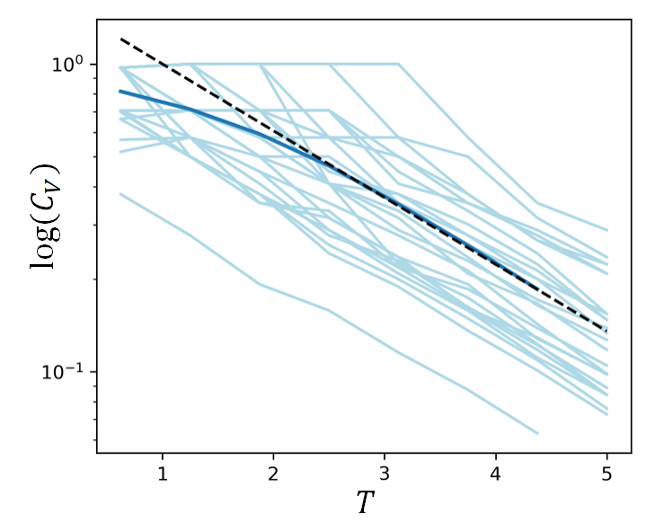
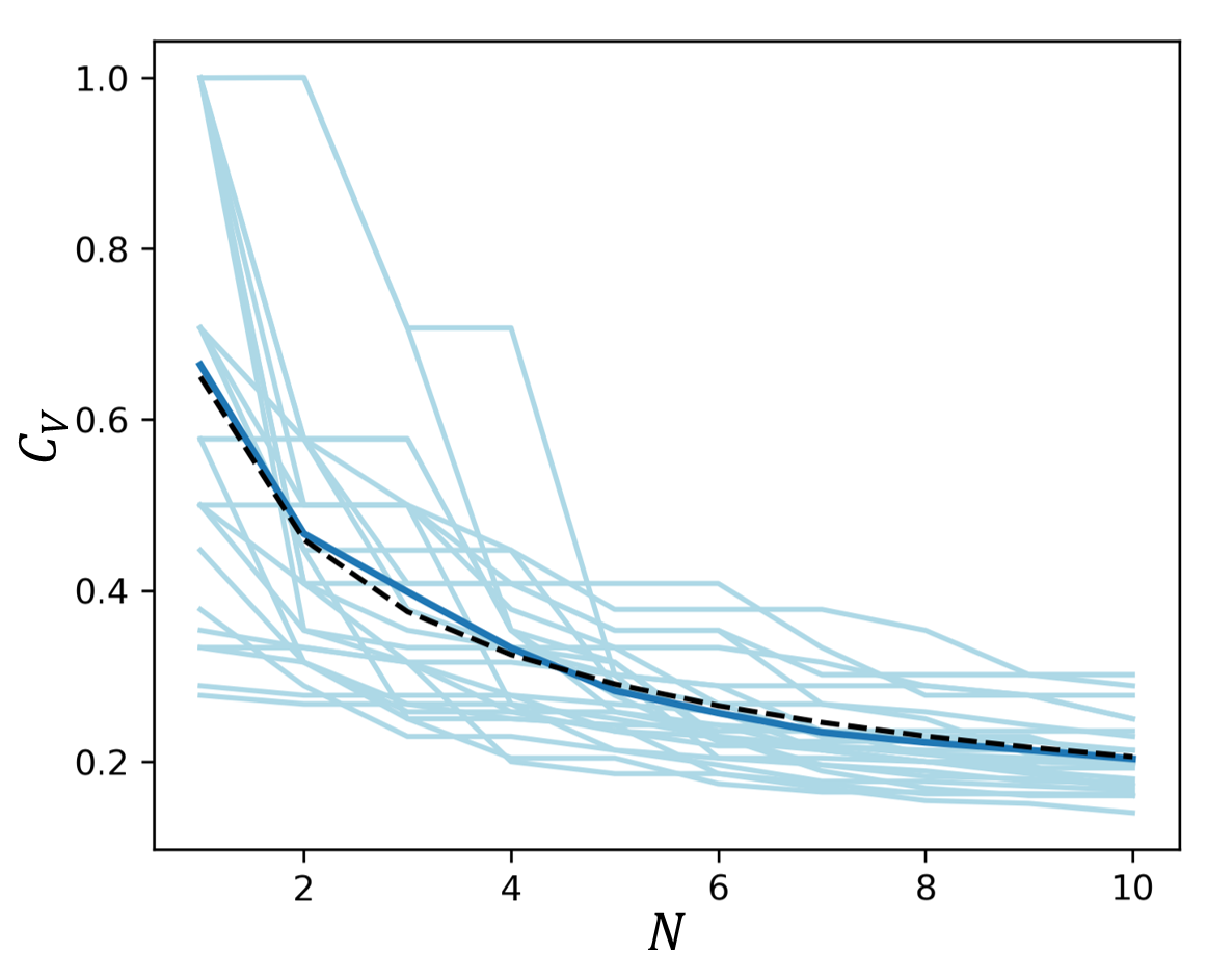
Since we do not know the full distribution of $r_{\nu}$ as a function of reaction constants $\boldsymbol{{\theta}}$ and $T$, we approximate the mean of the function in line 1 by the function of the mean in line 2 (mean-field approximation). This approximation works well as long as the function approximately scales linear with $\sum_{i}r_{\nu,i}$ in the range in which $p(\sum_{i}r_{\nu,i})\gg 0$. If we assume $\sum_{i}r_{\nu,i}$ is sufficiently large and the spread of $p(\sum_{i}r_{\nu,i})\gg 0$ is not too large, this mean-field approximation should work sufficiently well. We also used $n\langle r_{\nu}\rangle\gg a_{\nu}$ in line 3, since we are interested in the asymptotic behaviour $n\rightarrow\infty$. The scaling of $\langle c_{v}\rangle$ with ensemble size $n$ is shown in Figure 1b for rate constant $\theta_{1}$ of Model C. The proposed $n^{-1/2}$ scaling coincides with the ensemble mean of $c_{v}$ surprisingly well, despite the mean-field approximation.

C.2 Varying observation period T

We are now interested how the COV $c_{v}$ scales with observation period $T$. For a single trajectory, $\langle c_{v}\rangle\approx\langle r_{k}\rangle^{-1/2}$ (see 15), where we assumed $\langle r_{\nu}\rangle\gg a_{\nu}$ since we are interested in the asymptotic behaviour $T\rightarrow\infty$. We therefore need to derive an expression for the mean number of observed reactions $\langle r_{\nu}\rangle$. We have defined reaction events as a Poisson process with transition rate $h_{\nu}$. The transition rates $h_{\nu}\propto N_{\nu}$ depend on the current population $N_{\nu}$, which change with every occurred reaction. To make some progress, we may approximate this process by replacing the current population $N_{\nu}$ with its mean value $\langle N_{\nu}\rangle(t)$. The resulting process is a Poisson process with time dependent transition rate $h^{*}_{\nu}=\theta_{\nu}\cdot\langle N_{\nu}\rangle(t)$, also called Inhomogenous Poisson Process. In this case, the total number of reactions $r_{k}$ is Poisson distributed [2]:

$$p(r_{\nu})\approx\frac{(\Lambda)^{r_{\nu}}}{{r_{\nu}!}}e^{-\Lambda}\quad\text{with}\Lambda:=\int_{0}^{T}h^{*}_{\nu}(t)dt=\theta_{\nu}\int_{0}^{T}\langle N_{\nu}\rangle(t)dt,$$ (16)

with mean $\langle r_{\nu}\rangle=\Lambda$. The mean COV for an ensemble of $n$ trajectories is therefore:

$$\langle c_{v}\rangle(\theta_{\nu}|\xi_{1},\ldots,\xi_{n})\approx\frac{1}{\sqrt{n\theta_{\nu}\int_{0}^{T}\langle N_{\nu}\rangle(t)dt}},$$ (17)

where the mean COV of $\theta_{\nu}$ depends explicitly on the rate constant itself (additionally, $\langle N_{\nu}\rangle$ may also depend on $\theta_{\nu}$). This result can be useful for experimental design again: a rough estimate for the magnitude of $\theta_{k}$ might be obtained from either prior knowledge or from a posteriors of quick trail runs. Equation (17) then allows us to estimate how long a full experiment should run in order to get parameter posteriors of desired precision.

C.3 Parameter estimation in Models C and U

As derived in equation (LABEL:mABX), the mean number of cells in state A in Model C,

$$\langle N_{A}\rangle(t)=N_{A0}e^{t\Delta\lambda},$$ (18)

either grows or decays over time, depending on the sign of $\Delta\lambda$. Combining equation (18) and (17), the asymptotic behaviour for $T\Delta\lambda\gg 1$ is given by:

$$\langle c_{v}\rangle(\theta_{k}|\xi_{1},\ldots,\xi_{n})\propto\left\{\begin{array}[]{ll}\frac{\exp\left(-T\Delta\lambda/2\right)}{\sqrt{N_{A0}n}}&\Delta\lambda>0,\\[10.0pt] \frac{1}{\sqrt{N_{A0}n}}&\Delta\lambda<0.\end{array}\right.$$ (21)

The posterior precision therefore does not increase with observation time $T$ if $\Delta\lambda<0$. This makes sense, since A-type cells will always die out for $\lambda_{BB}>\lambda_{AA}$ (see equation (LABEL:pext1)). The scaling of $\langle c_{v}\rangle$ with observation time $T$ is shown in Figure 1a for rate constant $\theta_{1}$ of Model C. The proposed exponential scaling $e^{-\Delta\lambda\cdot T/2}$ coincides well with the ensemble mean of $c_{v}$ for large observation times $T$. For small times $T$, both the mean-field approximation (15) and $T\Delta\lambda\gg 1$ break down.

(a)

(b)

Figure 1: Dependence of coefficient of variation of rate constant $\theta_{1}$ on observation time $T$ and ensemble size $N$. Trajectories were generated from Model C using parameters $(\theta_{1},\theta_{2},\theta_{3})=(1,1,0)$. (a) Dependence of $c_{v}$ on observation time $T$. Solid light-blue and dark blue lines show a set of trajectories and their mean, $\langle c_{v}\rangle$, respectively. The dashed black line shows the asymptotic expression given in equation (21). (b) Dependence of $c_{v}$ on ensemble size $N$. Solid light-blue and dark blue lines show a set of trajectories and their mean, $\langle c_{v}\rangle$, respectively. The dashed black line shows an $N^{-1/2}$ scaling.

We derived the following asymptotic behaviour of the means $\langle N_{A}\rangle$ for Model U:

$$\langle N_{A}\rangle(t),\langle N_{B}\rangle(t)\propto e^{(\alpha+\beta)t},$$ (22)

where $\alpha$ and $\beta$ are functions of rate constants $\boldsymbol{{\theta}}$ (see LABEL:mABY2). Since $\alpha+\beta\geq 0$, the mean populations always grow exponentially. Combining equations (22) and (17), the asymptotic behaviour for $(\alpha+\beta)T\gg 1$ is given by

$$\langle c_{v}\rangle(\theta_{k}|\xi_{1},\ldots,\xi_{n})\propto\frac{\exp\left(-(\alpha+\beta)T/2\right)}{n}.$$ (23)

Appendix D Sampling of trajectories with fixed endpoints

For sampling trajectories with fixed end points, we approximate the true stochastic process of Models C and U by an inhomogeneous Poisson process with time-dependent transition rates $h_{\nu}^{*}(t)$.

D.1 Proposing valid reaction numbers

This section closely follows the derivation presented in [3]. Let $\bi{r}$ be the vector whose entries $r_{\nu}$ are the number of $\nu$-type reactions occurring between two time points $t_{0}$ and $t_{1}$ with population snapshots $\bi{N}_{0}$ and $\bi{N}_{1}$, receptively. The stoichiometric matrix $\mathcal{S}_{l,k}$ denotes the change of population $l$ caused by reaction $k$. The reaction vector $\bi{r}$ therefore needs to fulfil the following equation:

$$\bi{N}_{1}=\bi{N}_{0}+\mathcal{S}\bi{r}\quad\Rightarrow\quad\mathcal{S}\bi{r}=\bi{N}_{1}-\bi{N}_{0}.$$ (24)

We assume that the stoichiometric matrix $\mathcal{S}$ is of full rank, since otherwise we can simplify the model by reducing the number of model dimensions. Then, we can partition the matrix $\mathcal{S}=(\tilde{\mathcal{S}},\mathcal{S}^{{}^{\prime}})$ where $\tilde{\mathcal{S}}$ is an invertible matrix. In the same way, we partition the reaction vector $\bi{r}=(\bi{\tilde{r}},\bi{r^{{}^{\prime}}})$, which yields:

$$\mathcal{S}\bi{r} = (\tilde{\mathcal{S}},\mathcal{S}^{{}^{\prime}})\left({\begin{array}[]{*{20}c}\bi{\tilde{r}}\\ \bi{r^{{}^{\prime}}}\end{array}}\right)=\tilde{\mathcal{S}}\bi{\tilde{r}}+\mathcal{S}^{{}^{\prime}}\bi{r^{{}^{\prime}}}=\bi{N}_{1}-\bi{N}_{0}$$ (27)

$$\Rightarrow\qquad\bi{\tilde{r}} = \tilde{\mathcal{S}}^{-1}\left[\bi{N}_{1}-\bi{N}_{0}-\mathcal{S}^{{}^{\prime}}\bi{r^{{}^{\prime}}}\right].$$ (28)

A good strategy for proposing valid reaction numbers $\bi{r}$ is therefore the following: Starting from a valid solution $\bi{r}$, we first randomly perturb reaction numbers corresponding to $\bi{r}^{{}^{\prime}}$ in an arbitrary way, and then calculate the residual elements $\bi{\tilde{r}}$ accordingly to (28). Since solutions of equation (28) are not necessarily always positive, we have to make sure that all elements of $\bi{r}$ are non-negative, otherwise we reject the proposal immediately.

D.2 Sampling reaction times

Given a reaction vector $\bi{r}$ with $r_{k}$ being the numbers of type-$k$ reactions, we sample the corresponding $r_{k}$ reaction times $0\leq\tau_{j}\leq\Delta t$ from an an inhomogeneous Poisson process with transition rate $h_{k}^{*}(t)$ [4].

Since populations $\bi{N}(0)$, $\bi{N}(\Delta t)$ are known at the end points of the trajectory, so are the transition rates $h_{k}^{*}=\theta_{k}\cdot N_{k}$. The question is now: how should the transition rates $h_{k}^{*}(t)$ vary between these values to accurately approximate the true process? Because we know that mean populations $\langle N_{k}\rangle(t)$ are either constant, exponentially growing or decaying, a natural choice for $h_{k}^{*}(t)$, $0\leq t\leq\Delta t$ would be an exponential function:

$$h_{k}^{*}(t)=\theta_{k}\cdot N_{k}(0)\left(\frac{N_{k}(T)}{N_{k}(0)}\right)^{t/\Delta t}.$$ (29)

D.3 Setting up the acceptance ratio

The Poisson approximation step is taken into account by selecting an appropriate Metropolis-Hastings acceptance probability, ensuring that the MCMC output is actually drawn from the correct posterior (see Metropolis-Hastings-Green Algorithm in [5]). To construct the acceptance probability, we require the complete-data likelihood of trajectories $\xi$ in the inhomogeneous Poisson model $L_{A}(\xi|\boldsymbol{\theta})$. For arbitrary transition rates $h_{k}^{*}(t)$, the complete-data likelihood of $n$ reaction events in range $[0,\Delta t]$ is given by

$$L_{P}(\xi|\boldsymbol{\theta})=\left[\prod_{i=1}^{n}h_{\nu_{i}}^{*}(t_{i})\right]e^{-\Lambda_{0}(\Delta t)}\quad\text{with}\quad\Lambda_{0}(\Delta t):=\int_{0}^{\Delta t}h^{*}_{0}(t)dt,$$ (30)

where $h^{*}_{0}=\sum_{\nu}h^{*}_{\nu}$ is the combined transition rate and $\nu_{i}$ is the type of the $i$-th reaction. Plugging in the exponential transition rate (29) yields:

$$L_{P}(\xi|\boldsymbol{\theta})=\left[\prod_{i=1}^{n}\theta_{\nu_{i}}N_{\nu_{i}}(0)\left(\frac{N_{\nu_{i}}(T)}{N_{\nu_{i}}(0)}\right)^{t_{i}/\Delta t}\right]e^{-\Lambda_{0}(\Delta t)}$$

$$\text{with}\quad\Lambda_{0}(\Delta t)=\Delta t\sum_{k}\theta_{k}\frac{\Delta N_{k}}{\Delta\log(N_{k})},$$ (31)

where $\Delta N_{k}=N_{k}(\Delta t)-N_{k}(0)$ and $\Delta\log(N_{k})=\log(N_{k}(\Delta t))-\log(N_{k}(0))$. We are now ready to construct the Metropolis-Hastings step for updating trajectories $\xi$ with fixed endpoints on interval $[0,\Delta t]$. First we propose a new set of valid reaction numbers $\bi{r^{\star}}$ from a proposal distribution $f(\bi{r^{\star}}|\bi{r})$. We chose to update $\bi{r^{\star}}=\bi{r}+\zeta$ by adding to each element a random integer $\zeta$ drawn from a symmetric Skellam distribution [6] with variance $2\omega$. The tuning parameter $\omega$ was chosen such that the proposals $\bi{r^{\star}}$ are accepted on average with a probability of $\approx 30\%$. Then, conditional on $\bi{r^{\star}}$, we will sample a trajectory (reaction times $\tau^{\star}_{j}$) from the approximate Poisson process with exponential transition rates (29). The trajectory $\xi^{\star}:=\{\bi{r^{\star}},\tau^{\star}_{i}\}$ is then accepted with probability $\text{min}(1,A)$ with

$$A=\left[\frac{L_{\rm CD}(\xi^{\star}|\boldsymbol{{\theta}})}{L_{P}(\xi^{\star}|\boldsymbol{\theta})}\frac{q(\bi{r^{\star}})}{f(\bi{r^{\star}}|\bi{r})}\right]\left/\left[\frac{L_{\rm CD}(\xi|\boldsymbol{{\theta}})}{L_{P}(\xi|\boldsymbol{\theta})}\frac{q(\bi{r})}{f(\bi{r}|\bi{r^{\star}})}\right]\right.,$$ (32)

where $L_{\rm CD}$ is the complete-data likelihood of the true model (see (LABEL:LCD)) and $q(\bi{r})=\prod_{\nu}q_{\nu}(r_{\nu})$ is the probability that $\bi{r}$ reactions were observed in the inhomogeneous Poisson model. The terms $q_{\nu}$ are the PMF of the Poisson distribution:

$$q_{\nu}(r_{\nu})=\frac{\Lambda_{\nu}(\Delta t)^{r_{\nu}}}{r_{\nu}!}e^{-\Lambda_{\nu}(\Delta t)}\quad\text{with}\quad\Lambda_{\nu}(\Delta t)=\Delta t\cdot\theta_{\nu}\frac{\Delta N_{\nu}}{\Delta\log(N_{\nu})}.$$ (33)

Note that the the acceptance probability (32) depends on the current parameter vector $\boldsymbol{\theta}$, which is drawn at every iteration of the MCMC. The overall structure of this algorithm was originally motivated by [3] and modified by us to fitS Model c AND u. It is an application of the general Metropolis-Hastings-Green Algorithm as described in [5].

Appendix E Bayes factor calculation using population snapshots

E.1 The harmonic mean identity

For a given model $M$, some data $y$ and a parameter $\theta$, we have from Bayes’ theorem that

$$\frac{p(\boldsymbol{\theta}|M)}{p(\boldsymbol{\xi}|M)}=\frac{p(\boldsymbol{\theta}|\boldsymbol{\xi},M)}{p(\boldsymbol{\xi}|\boldsymbol{\theta},M)}\;.$$ (34)

Integrating both sides over $\boldsymbol{\theta}$ gives us the identity

$$\frac{1}{p(\boldsymbol{\xi}|M)}=\mathbb{E}\left[\left.\frac{1}{p(\boldsymbol{\xi}|\boldsymbol{\theta},M)}\right|\boldsymbol{\xi},M\right].$$ (35)

This is useful because the average is taken over the posterior distribution of the parameters $\boldsymbol{\theta}$, conditioned on a particular set of observations $\boldsymbol{\xi}$. This is exactly what the MCMC algorithm generates, and hence we can estimate the marginal likelihood $p\left(\{\boldsymbol{N}(t_{i})\}|M\right)$ as

$$\hat{p}(\{\boldsymbol{N}(t_{i})\}|M)=\left[\frac{1}{B}\sum_{m=1}^{B}\frac{1}{L_{SS}(\{\boldsymbol{N}(t_{i})\}|\boldsymbol{\theta}^{m})}\right]^{-1}\;,$$ (36)

where $\boldsymbol{\theta}^{m}$ is the $m^{\rm th}$ sample of the parameter vector obtained from the MCMC algorithm. Unfortunately, the snapshot likelihood $L_{SS}(\{\boldsymbol{N}(t_{i})\}|\boldsymbol{\theta}^{m})$ needs to be evaluated by a Monte Carlo (MC) estimate for each parameter vector $\boldsymbol{\theta}^{m}$ separately by:

$$\hat{L}_{SS}(\{\boldsymbol{N}(t_{i})\}|\boldsymbol{\theta}^{m})=\frac{1}{B^{{}^{\prime}}}\sum_{k=1}^{B^{{}^{\prime}}}\delta(\{\boldsymbol{N}(t_{i})-\boldsymbol{N}^{sim}_{k}(t_{i})\}),$$ (37)

where $\boldsymbol{N}^{sim}_{k}(t_{i})$ is a simulated trajectory from the respective model with parameters $\boldsymbol{\theta}^{m}$. The delta function $\delta(\cdot)$ equals one if simulated and observed populations coincide at snapshot times. This resulting in a computationally intense MC within MCMC algorithm, which is however still less computationally intensive than the other presented methods (thermodynamic integration, product space search).

E.2 Thermodynamic integration

Thermodynamic integration is another method to estimate marginal likelihoods of models. It is based on the fact that the logarithm of the marginal likelihood can be represented by the following integral [7]:

$$\log p(\boldsymbol{\xi})=\int_{0}^{1}\mathbb{E}_{\boldsymbol{\theta}|\boldsymbol{\xi},t}\left[\log p(\boldsymbol{\xi}|\boldsymbol{\theta})\right]dt,$$ (38)

with $\boldsymbol{\xi}$ being general data, $p(\boldsymbol{\theta})$ the parameter prior, $p(\boldsymbol{\xi}|\boldsymbol{\theta})$ the likelihood and $p(\boldsymbol{\xi})$ the marginal likelihood. The distribution used to evaluate the mean $E_{\boldsymbol{\theta}|\boldsymbol{\xi},t}[\cdot]$ is called power-posterior $p_{t}(\boldsymbol{\theta}|\boldsymbol{\xi})$ with temperature $t\in[0,1]$, defined as [8]:

$$p_{t}(\boldsymbol{\theta}|\boldsymbol{\xi}):=\frac{p(\boldsymbol{\xi}|\boldsymbol{\theta})^{t}q(\boldsymbol{\theta})}{\int p(\boldsymbol{\xi}|\boldsymbol{\theta})^{t}q(\boldsymbol{\theta})d\boldsymbol{\theta}}.$$ (39)

The power-posterior can be interpreted as an intermediate distribution between prior and posterior, since $p_{t=0}(\boldsymbol{\theta}|\boldsymbol{\xi})=p(\boldsymbol{\theta})$ and $p_{t=1}(\boldsymbol{\theta}|\boldsymbol{\xi})=p(\boldsymbol{\theta}|\boldsymbol{\xi})$. For derivations and evaluation techniques of the integral (38), see [7].

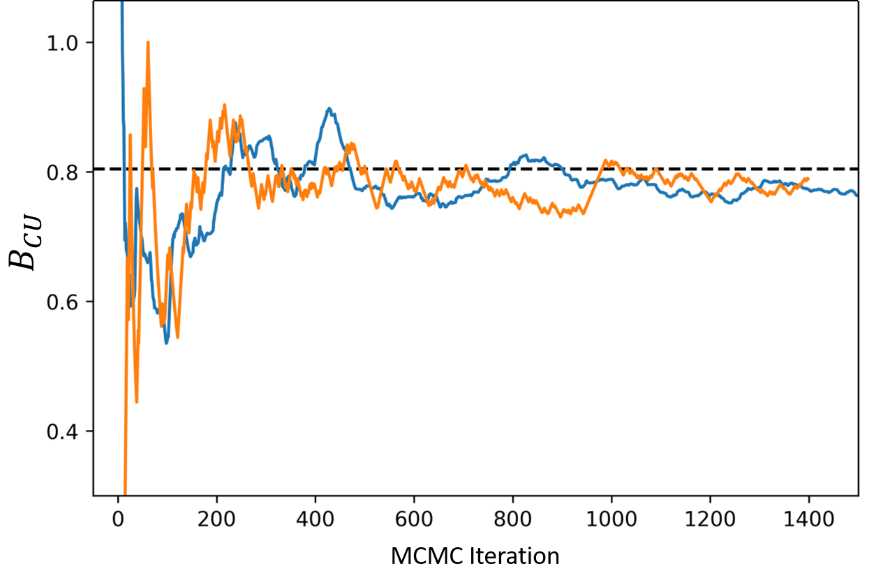
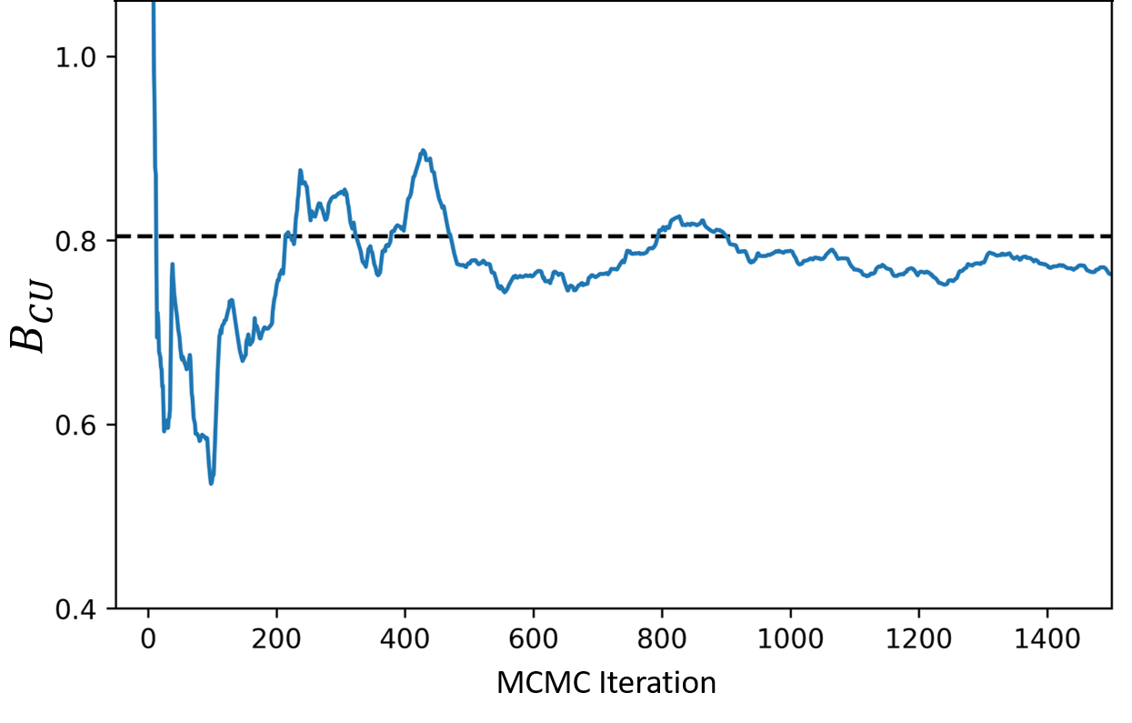
The Bayes factor calculation via thermodynamic integration is usually very accurate. On the other hand, it is computationally even more intensive than the harmonic mean identity and also more complicated to implement. We therefore try to avoid thermodynamic integration if other methods provide equally good estimates. As an example, Figure 2 compares the Bayes factors obtained via the harmonic mean estimator (36) and via thermodynamic integration given two population snapshots. The harmonic mean estimator converges quite fast and provides equally good Bayes factor estimates than the method of thermodynamic integration.

Figure 2: Calculation of Bayes factor $B_{CU}$ using the harmonic mean identity (solid blue line) and thermodynamic integration (dashed black line) given two snapshots $\bi{N}(0)=(3,3)$, $\bi{N}(1)=(8,8)$ and flat priors $\theta_{\nu}\mathrel{\stackrel{{\scriptstyle\makebox[0.0pt]{\mbox{\tiny iid}}}}{{\sim}}}\mathcal{U}[0,3]$ for Models C and U. The harmonic mean estimate (36) converges after only $B\approx 300$ MCMC iterations, although the convergence speed strongly depends on the snapshot data and on the sample size of the MC-step for estimating the snapshot-likelihood $L_{SS}(\{\bi{N}(t_{i})\}|\boldsymbol{\theta})$. We use thermodynamic integration only to estimate convergence speed, since this calculation is much more intensive than the harmonic mean identity.

E.3 Product space search

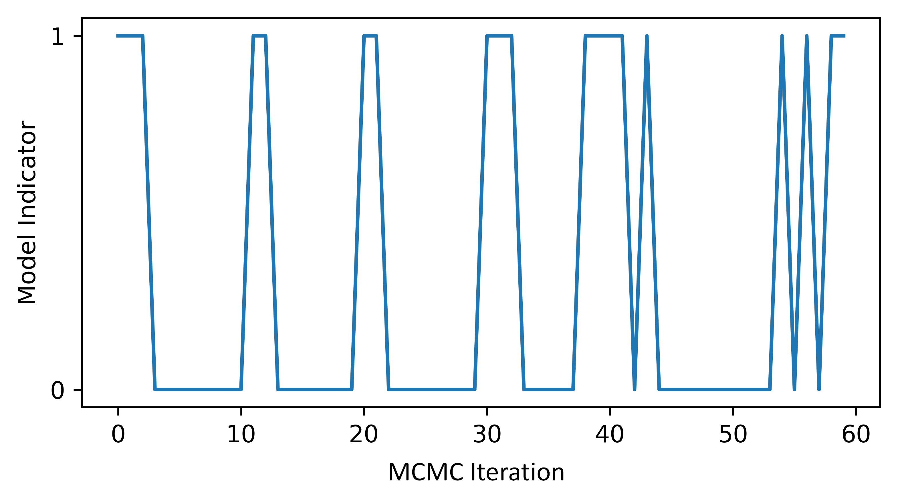
Another popular method to obtain Bayes factors is the product space search [9]. Whereas the harmonic mean identity and thermodynamic integration are used to estimate the marginal likelihoods of Models C and U, the product space search estimates $B_{CU}$ directly. This method involves an MCMC algorithm not only exploring the parameter space of a single model, but jumping between competing models. In general, jumps between a whole set of competing models $\{M_{j}\}$ are allowed, but we will allow the algorithm to switch only between Models C and U. At the start of each iteration, we either stay in the current model or jump to the other model with a certain probability. In the end, the Bayes factor $B_{CU}\approx N(M=C)/N(M=U)$ can be estimated by the ratio of times the MCMC stayed in either Model C or Model U (see Figure 3 (a)).

(a)

(b)

Figure 3: Calculation of Bayes factor $B_{CU}$ using product space search given two snapshots $\bi{N}(0)=(3,3)$, $\bi{N}(1)=(8,8)$ and flat priors $\theta_{\nu}\mathrel{\stackrel{{\scriptstyle\makebox[0.0pt]{\mbox{\tiny iid}}}}{{\sim}}}\mathcal{U}[0,3]$ for Models C and U. (a) MCMC jumping between different Model C ($0$) and U ($1$) over a range of MCMC iterations. The Bayes factor can be estimated by the ratio of times the MCMC stayed in either Model C or Model U. (b) Estimation of $B_{XY}$ using product space search (solid orange line), the harmonic mean estimator (solid blue line) and thermodynamic integration (dashed black line).

We implement the product space search following [10, “Metropolised Carlin and Chib”]. The performance of this method is compared to the harmonic mean estimator in Figure 3(b). Both methods have similar convergence speeds and variances. This is surprising, since the harmonic mean estimator has been criticised for being the “Worst Monte Carlo Method Ever” [11]. The reason being that although it is a consistent estimator, it may have infinite variance in some cases. This could not be observed in our system, where it has similar variance than more sophisticated methods such as the product space search.

(a) $\lambda_{AA}$-$\lambda_{AB}$-space

(b) $\lambda_{AB}$-$\lambda_{BB}$-space

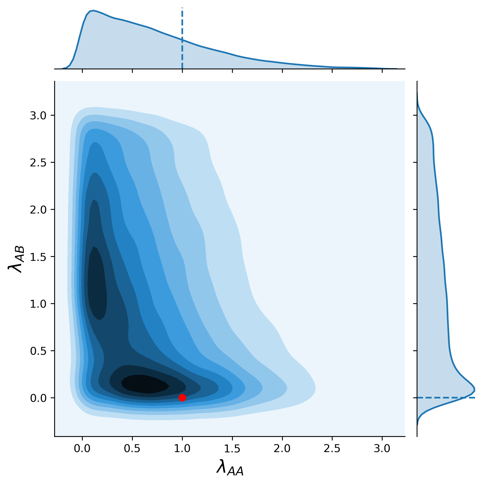
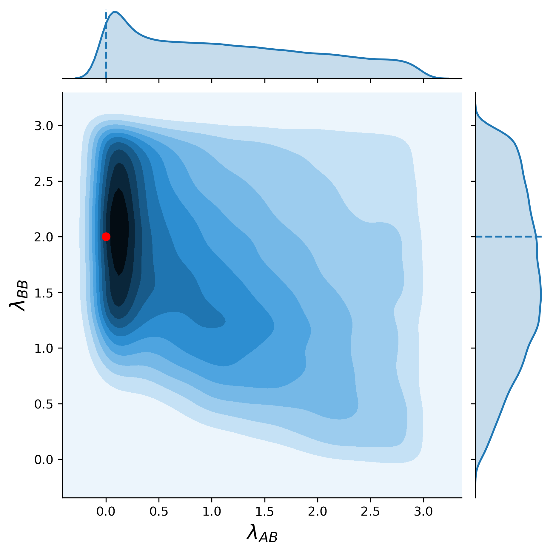
Figure 4: Posterior distribution of Model C calculated based on five independent snapshots $\{\boldsymbol{N}(t=1.0)\}$ which were sampled from a system with parameters $\boldsymbol{\theta}=(1,0,2)$ with initial conditions $\boldsymbol{N}(t=0)=(5,5)$, and uniform, independent priors $\theta_{\nu}\mathrel{\stackrel{{\scriptstyle\makebox[0.0pt]{\mbox{\tiny iid}}}}{{\sim}}}\mathcal{U}[0,3]$. The three-dimensional posterior for Model C is projected onto the two-dimensional planes with the corresponding marginal probability distributions at upper and right margins, shown as the KDE of MCMC samples. The true rate constants from which the two snapshot data were created is shown as a red dot and dashed, blue lines. The non-zero posterior density for negative rate constants is due to the KDE visualisation and does not represent actual points sampled by the MCMC. Because the population dynamics in model C are less sensitive to changes in the asymmetric division rate $\lambda_{AB}$ than to variations in $\lambda_{AA}$ and $\lambda_{BB}$, we observe a larger posterior variance along $\lambda_{AB}$.

Appendix F Supplementary figures for ABC of epiblast stem cell data

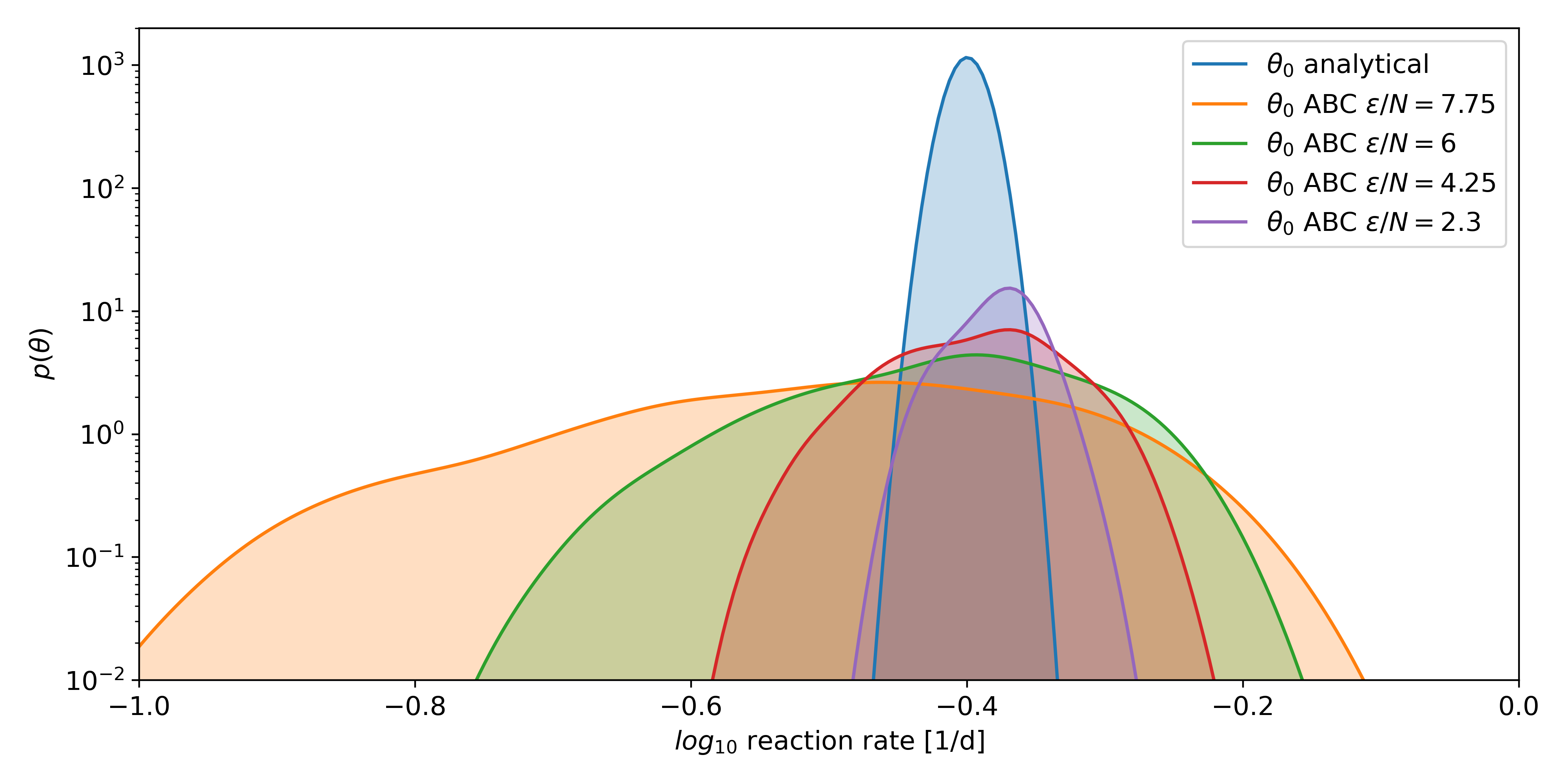
Figure 5: Comparison of SMC-ABC posterior distributions $p(\boldsymbol{\theta}|D(s(\mathcal{D}^{sim}),s(\mathcal{D}))<\epsilon)$ and the analytical posterior distribution $p(\theta_{0}|\mathcal{D})$ of model U obtained from dataset $\mathcal{D}_{\mathrm{CHIR}}$. For sufficiently small $\epsilon$, the SMC-ABC posterior deviates only slightly from the exact solution. For this specific case, the analytical posterior distribution can be calculated because the likelihood for $\theta_{0}$ in model U is known: $p(\theta_{0}|N)=e^{-\theta_{0}t}(1-e^{-\theta_{0}t})^{N-1}$, which is the probability that we observe a clone size of $N$ cells at time $t$.

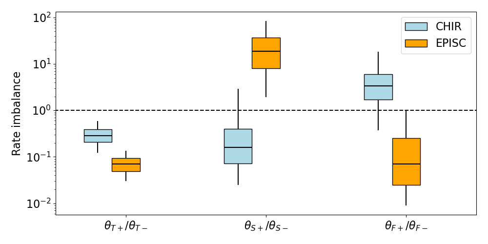
Figure 6: Median (horizontal line), 0.25/0.75 quantiles (box) and 0.05/0.95 quantiles (vertical lines) of the rate imbalance of Model U log-rates $\log_{10}(\theta_{k})$ obtained from $\mathcal{D}_{\mathrm{CHIR}}$ and $\mathcal{D}_{\mathrm{EPISC}}$.

(a) CHIR conditions

(b) EPISC conditions

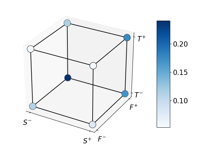
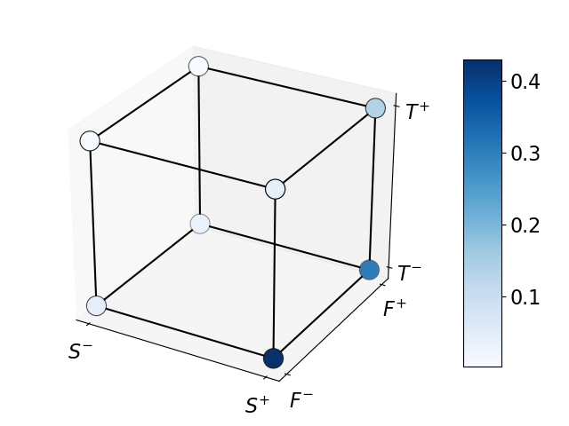
Figure 7: Complete cell state distribution of initially unsorted stem cells after $t=3d$ for different environmental conditions (CHIR/EPISC). The initial cell state distribution at $t=0d$ is assumed to be uniform. The probability of the respective marker expression is indicated by the color map.

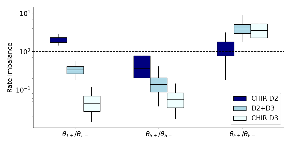
Figure 8: Median (horizontal line), 0.25/0.75 quantiles (box) and 0.05/0.95 quantiles (vertical lines) of the rate imbalance of Model U log-rates $\log_{10}(\theta_{k})$ obtained from $\mathcal{D}_{\mathrm{CHIR}}$. CHIR D2 and CHIR D3 shows inferred parameters using exclusively day 2 or day 3 data, respectively. CHIR D2+D3 was obtained by including all data points of $\mathcal{D}_{\mathrm{CHIR}}$.

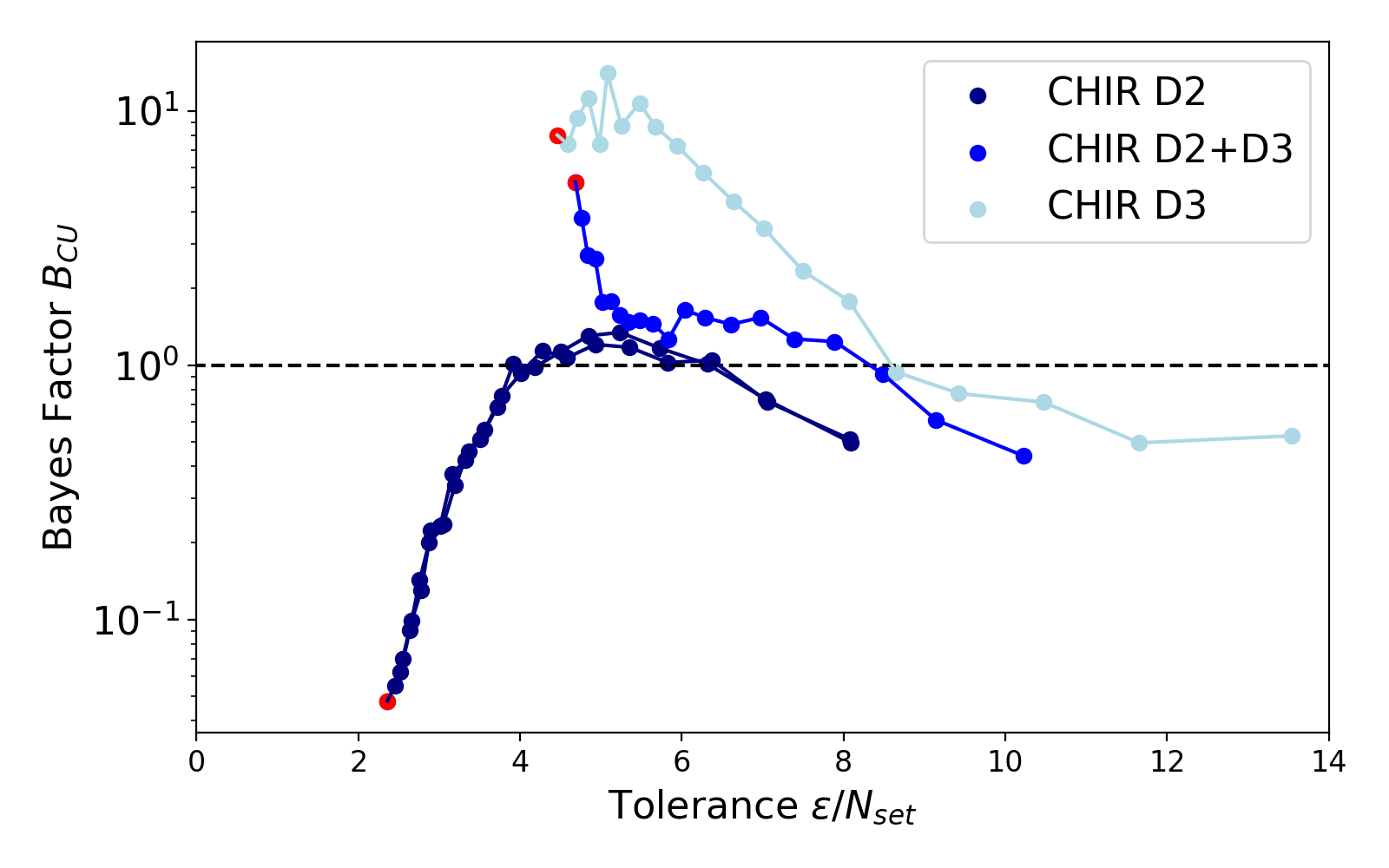
Figure 9: Bayes factors $B_{CU}$ of dataset $\mathcal{D}_{\mathrm{CHIR}}$ using either exclusively day 2 or day 3 data over a range of tolerance values $\epsilon$. Identical log-uniform priors were used for all rate constants in both models $\log_{10}(\theta_{k})\sim\mathcal{U}[-2,0])$. The x-axis was re-scaled by the number of measurement series $N_{set}$ ($N_{set}=4$ for both D2 and D3). Red dots show the minimal epsilon value to which the SMC-ABC algorithm converged after $20$ iterations. The data up to day 2 favours model C dynamics ($B_{CU}>1$) while the population data at day 3 provides evidence in favour for model U dynamics ($B_{CU}<1$).

Appendix G Rejection-ABC given experimental stem-cell data

We used the following Rejection-ABC algorithm to verify results for parameter inference and model selection (modified from [12]). The advantage of this algorithm is that it samples the entire parameter space uniformly and therefore does not risk getting stuck in local minima, unlike MCMC and SMC algorithms. Since Rejection-ABC is less efficient than SMC-ABC, calculations with this algorithm are only feasible at larger tolerance values $\epsilon$.

Algorithm 1 Rejection-ABC for model selection

1:  Set model $M^{\star}=M_{C}$ with probability $0.5$, otherwise set $M^{\star}=M_{U}$

2:  Sample parameter $\boldsymbol{\theta}^{\star}$ according to prior distribution $q(\boldsymbol{\theta}^{\star}|M^{\star})$

3:  Simulate a set of trajectories $\{\xi\}$ from $M^{\star}$ with parameters $\boldsymbol{\theta}^{\star}$ and obtain projected snapshot data $D^{sim}$

4:  If $D(s(\mathcal{D}^{sim}),s(\mathcal{D}))<\epsilon$, accept $(\boldsymbol{\theta},M^{\star})$, otherwise reject

5:  Go back to (1)

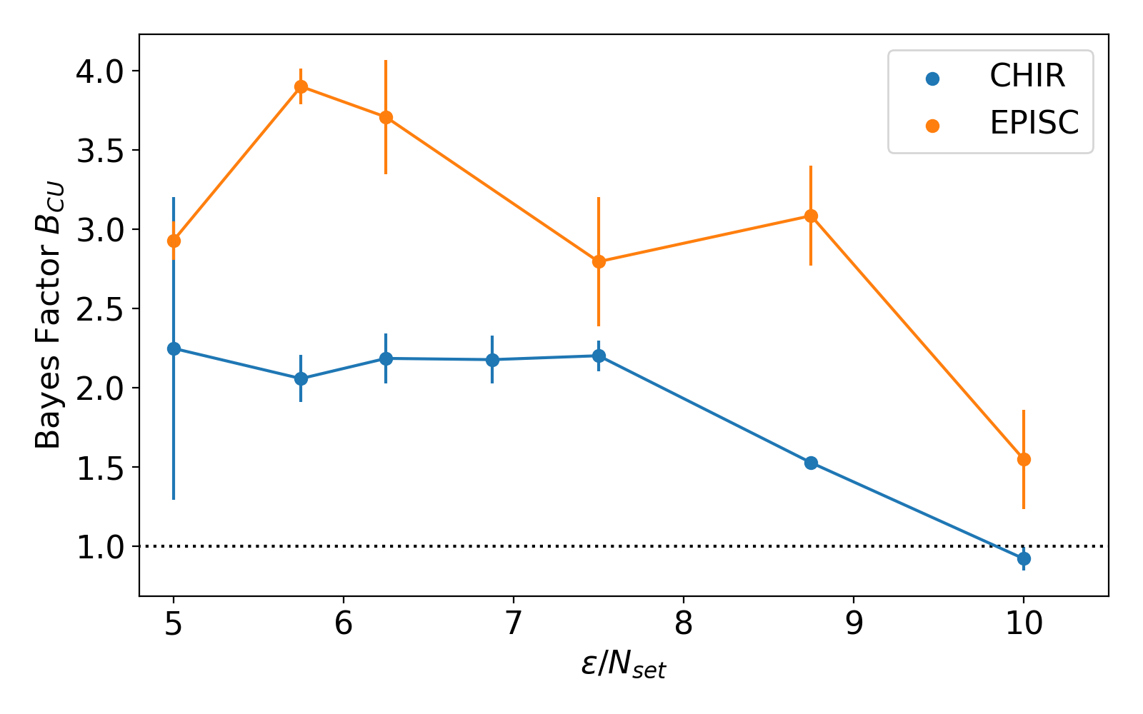
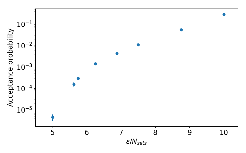
The rejection-ABC algorithm was run several times and $\epsilon$ was progressively lowered until the acceptance probability of samples reached a lower threshold of $10^{-5}$. While lowering $\epsilon$, the acceptance probability decreases faster than exponentially (see Figure 11 a). The Bayes factor $B_{CU}$ can be estimated by the ratio of the acceptance probabilities of models $M_{C}$ and $M_{U}$. This was done for both datasets $\mathcal{D}_{\mathrm{CHIR}}$ and $\mathcal{D}_{\mathrm{EPISC}}$ and the resulting Bayes factors are shown in Figure 11 b as a function of $\epsilon$. We chose identical log-uniform priors for all rate constants in both models $\log_{10}(\theta_{k})\sim\mathcal{U}[-3,1])$ (in units of per day). Note that these priors have a slightly larger domain than the ones used for SMC-ABC.

For large $\epsilon$, the resulting posterior distributions differ only slightly from the uniform priors and Model C and Model U are equally likely ($B_{CU}\approx 1$). By decreasing $\epsilon$, the posterior distributions show distinct peaks and are very different for both models. Consequently by lowering $\epsilon$, $B_{CU}$ starts to deviate from one and eventually plateaus at a finite value $B_{CU}>1$. The large uncertainty for $\epsilon/N_{set}=5$ is due to a very low acceptance probability, leading to a small sample size of accepted parameters.

Figure 10: Mean and standard deviation of Model C log-rates $\log_{10}(\theta_{k})$ calculated from posterior distributions given $\mathcal{D}_{\mathrm{CHIR}}$ using Rejection-ABC. Replacing the $L_{1}$-norm in eqn (LABEL:diff_norm) by the $L_{2}$-norm does not significantly change the shape of parameter posteriors given $\epsilon$ is small enough ($\epsilon/N_{set}=5$ used for $L_{1}$ and $\epsilon/N_{set}=3$ used for $L_{2}$).

(a) Acceptance probability as a function of tolerance $\epsilon$ for Model C and dataset $\mathcal{D}_{\mathrm{CHIR}}$.

(b) Bayes factors $B_{CU}$ of datasets $\mathcal{D}_{\mathrm{CHIR}}$ and $\mathcal{D}_{\mathrm{EPISC}}$ for a range of tolerance values $\epsilon$.

Figure 11: Acceptance probability and Bayes factors for a range of tolerance values $\epsilon$ with identical log-uniform priors for all rate constants in both models $\log_{10}(\theta_{k})\sim\mathcal{U}[-3,1])$. The x-axis was re-scaled by the number of measurement series $N_{set}$ in the respective dataset ($N_{set}=8$ in $\mathcal{D}_{\mathrm{CHIR}}$, $N_{set}=4$ in $\mathcal{D}_{\mathrm{EPISC}}$). Errorbars indicate the spread between five independent rejection-ABC runs.

References

• [1] N.L. Johnson, A.W. Kemp, and S. Kotz. Univariate discrete distributions, volume 444. John Wiley & Sons, 2005.
• [2] S.M. Ross, J.J. Kelly, R.J. Sullivan, W.J. Perry, D. Mercer, R.M. Davis, T.D. Washburn, E.V. Sager, J.B. Boyce, and V.L. Bristow. Stochastic processes, volume 2. Wiley New York, 1996.
• [3] D.J. Wilkinson. Stochastic modelling for systems biology. CRC press, 2011.
• [4] R. Pasupathy. Wiley Encyclopedia of Operations Research and Management Science, chapter Generating Nonhomogeneous Poisson Processes. John Wiley and Sons, Inc., 2011.
• [5] S. Brooks, A. Gelman, G. Jones, and X.-L. Meng. Handbook of Markov Chain Monte Carlo. CRC press, 2011.
• [6] N.L. Johnson and S. Kotz. Discrete distributions: Distributions in statistics. Houghton Mifflin, 1969.
• [7] B. Calderhead and M. Girolami. Estimating bayes factors via thermodynamic integration and population mcmc. Comput. Stat. Data Anal., 53(12):4028–4045, 2009.
• [8] N. Friel and A.N. Pettitt. Marginal likelihood estimation via power posteriors. J. Royal Stat. Soc. B, 70(3):589–607, 2008.
• [9] S. Chib. Marginal likelihood from the gibbs output. J. Am. Stat. Assoc., 90(432):1313–1321, 1995.
• [10] P. Dellaportas, J.J. Forster, and I. Ntzoufras. On Bayesian model and variable selection using MCMC. Stat. Comput., 12(1):27–36, 2002.
• [11] A.E. Raftery, M.A. Newton, J.M. Satagopan, and P.N. Krivitsky. Estimating the integrated likelihood via posterior simulation using the harmonic mean identity, volume 8 of Bayesian Statistics, pages 1–45. Oxford University Press, 2006.
• [12] T. Toni, D. Welch, N. Strelkowa, A. Ipsen, and M.P.H. Stumpf. Approximate Bayesian computation scheme for parameter inference and model selection in dynamical systems. J. R. Soc. Interface, 6(31):187–202, 2008.