Predictions of the $L_{\rm[CII]}$– SFR and [CII] Luminosity Function at the Epoch of Reionization

Abstract

We present the first predictions for the $L_{\rm[CII]}$– SFR relation and [CII] luminosity function (LF) in the Epoch of Reionization (EoR) based on cosmological hydrodynamics simulations using the simba suite plus radiative transfer calculations via sígame. The sample consists of 11,137 galaxies covering halo mass $\log$ M${}_{\rm halo}\in[9,12.4]$ $M_{\odot}$, star formation rate SFR$\in[0.01,330]$ $M_{\odot}$  yr^-1, and metallicity $\langle Z_{\rm gas}\rangle_{\rm SFR}\in[0.1,1.9]\,Z_{\odot}$. The simulated $L_{\rm[CII]}$-SFR relation is consistent with the range observed, but with a spread of $\simeq$ 0.3 dex at the high end of SFR ($>$ 100 $M_{\odot}$  yr^-1) and $\simeq$0.6 dex at the lower end, and there is tension between our predictions and the values of $L_{\rm[CII]}$ above 10^8.5 $L_{\odot}$ observed in some galaxies reported in the literature. The scatter in the $L_{\rm[CII]}$– SFR relation is mostly driven by galaxy properties, such that at a given SFR, galaxies with higher molecular mass and metallicity have higher $L_{\rm[CII]}$. The [CII] LF predicted by simba is consistent with the upper limits placed by the only existing untargeted flux-limited [CII] survey at the EoR and those predicted by semi-analytic models. We compare our results with existing models and discuss the differences responsible for the discrepant slopes in the $L_{\rm[CII]}$– SFR relation.

1. Introduction

Deep field surveys carried out with the Hubble Space Telescope have enabled the detection of galaxies out to the cosmic dawn at $z$ $\gtrsim\,$11 and provide stringent constraints on the bright end of rest-frame UV luminosity functions (LF) of galaxies during the Epoch of Reionization (e.g., Oesch et al. 2016; Song et al. 2016; Finkelstein 2016). While measuring distributions of galaxy properties, such as the LF, provides important constraints on how galaxies evolve over cosmic time, it is also useful to target individual sources at high redshift in order to conduct detailed case studies. Such studies allow us to address open questions such as properties of the interstellar medium (ISM), how metal enrichment in galaxies proceded in the early universe, how much star formation is dust-obscured or how much dust is present in these early systems, and the physical conditions under which star formation and stellar mass assembly took place. Follow-up observations with the Atacama Large (Sub-)Millimeter Array (ALMA) probing the dust continuum and line emission from ions and molecules in the dense ISM of high-redshift galaxies appear extremely promising for characterizing the star-forming gas and dust properties of early galaxies and helping to constrain the physical processes at play (see a review by Hodge & da Cunha 2020).

Owing to the relative brightness of the fine-structure line from singly ionized carbon at rest-frame 157.7 $\mu$m and accessibility of the line with ALMA at high redshift, there is currently great interest in using [CII] line emission as a tracer to study galaxies during the Epoch of Reionization (EoR). At the moment, most of these follow-up observations target some of the brightest objects samples selected at other wavelengths (e.g., Capak et al. 2015; Smit et al. 2018; Marrone et al. 2018). [CII] has been detected in a handful of normal star-forming galaxies at the EoR (e.g., Capak et al. 2015; Carniani et al. 2018a) and even resolved on kpc-scales to study the gas kinematics for a handful of sources (e.g., Jones et al. 2017; Matthee et al. 2017; Carniani et al. 2018a; Hashimoto et al. 2019). However, due to the small field of view of ALMA, it is extremely challenging and expensive to carry out flux-limited (untargeted) surveys over significant areas. The largest area untargeted survey to date that probes [CII] at $z\sim 6-8$ is the ALMA Spectroscopic Survey in the HUDF (Large Program; ASPECS), which covers 4.6 arcmin² (Walter et al. 2016; Aravena et al. 2016).

While these detections are exciting, interpretation of the [CII] line luminosity and its connection with galaxy properties remains complex and poorly understood. [CII] is the dominant coolant in the ISM in nearby star forming galaxies, and its luminosity is expected to be correlated with the star formation rate (SFR). Indeed, such a correlation is seen in local galaxies (De Looze et al. 2014; Herrera-Camus et al. 2015), but with hints that the $L_{\rm[CII]}$/SFR ratio depends on other galaxy properties such as metallicity and dust temperature (e.g. Malhotra et al. 2001; Luhman et al. 2003; Díaz-Santos et al. 2014). This is expected, as the dust content affects the degree of shielding against hard ionizing photons, as well as the amount of photoelectric heating, which affect the ionization state of the line emitting gas and the collision rate. In addition, theoretical modeling has shown that $L_{\rm[CII]}$/SFR is also expected to depend on the pressure of the ISM environment, if molecular cloud sizes depend on the ambient pressure, and on the density distribution on small scales within the ISM (Popping et al. 2019).

Another motivation for studying the physics of line emission and its connection to galaxy properties and the physics of galaxy formation is the development of multiple experiments that will carry out line intensity mapping (LIM) studies. Different LIM experiments will enable the detection of various tracers of dense and more diffuse gas in and around galaxies, including Lyman-$\alpha$, H$\alpha$, 21-cm, CO, and [CII] (see Kovetz et al. 2017 for a review). LIM promises to map the statistical signal from emission in galaxies over very large volumes (on the order of Mpc-to-Gpc-scales), with the tradeoff of not resolving individual galaxies. As such, LIM experiments also probe emission from faint galaxies. While LIM holds great promise for studying galaxy evolution and cosmology (e.g., the cosmic star formation history, evolution of the ISM and intergalactic medium (IGM), and physical processes during the EoR; Kovetz et al. 2017), the power spectra depend on the line luminosities of different galaxy populations within the volume sampled (or the intrinsic line LF). Therefore, physically motivated models that can self-consistently predict line luminosities are vital for strategizing LIM experiments and interpreting LIM data. As shown by Yue & Ferrara (2019), a shallower $L_{\rm[CII]}$  – SFR relation would imply that the [CII] LF drops quickly at the bright end and most of the IM signal comes from faint galaxies. This in turn determines the detection depth needed for [CII] LIM experiments. At the moment, most LIM forecasts for tracers such as CO and [CII] have been made using a series of empirical scaling relations (e.g., Gong et al. 2012; Uzgil et al. 2014; Keating et al. 2015; Chung et al. 2019).

Carrying out detailed and realistic predictions of the [CII] emission for a large cosmologically representative sample of galaxies is extremely challenging. The [CII] line can arise from all phases of the ISM, by being collisionally excited by either electrons, atoms or molecules. Hence, the line strength depends strongly on the density and kinematic temperature of these species. Modeling has repeatedly shown that different ISM phases are all important to consider when deriving [CII] emission for a galaxy (e.g., Olsen et al. 2017; Pallottini et al. 2019; Lupi & Bovino 2020). However, state-of-the-art cosmological simulations of volumes larger than 100 Mpc do not resolve particle masses below $\sim$ 10^6-7 $M_{\odot}$ (at $z$ = 0; e.g., Davé et al. 2019; Nelson et al. 2018), which corresponds to hydrogen densities below $n_{H}$ ¡ 100 ${\rm cm}^{-3}$ and temperatures above 10⁴ K. In particular the molecular ISM phase — with typical densities above a few hundred cm³ and and temperatures below 100 K — is not tracked in cosmological simulations but knowledge about it is critical in order to reliably simulate [CII] line emission. Currently, all large volume cosmological simulations adopt phenomenological “sub-grid” recipes to treat unresolved processes such as star formation, stellar feedback, and chemical enrichment, and these carry significant uncertainties (see review by Somerville & Davé 2015). Additionally, a second type of “sub-grid” modeling is required to describe the detailed structures of molecular gas on cloud scales, which must be input into the radiative transfer (RT) and ionization state modeling tools described in more detail below.

Previous works that have attempted to model [CII] for galaxy populations mainly fall into three categories: (i) extremely simple, empirical mappings between $L_{\rm[CII]}$ and halo mass (Visbal & Loeb 2010; Gong et al. 2012), (ii) semi-analytic models to predict galaxy properties coupled with machinery to predict the [CII] emission in post-processing (Popping et al. 2016; Lagache et al. 2018; Popping et al. 2019), or (iii) small samples of cosmological zoom-in simulations again post-processed to compute the radiative transfer and line emission (Olsen et al. 2015; Narayanan et al. 2015; Vallini et al. 2015; Olsen et al. 2017; Katz et al. 2017; Pallottini et al. 2017b, a). A few recent studies have coupled on-the-fly radiative transfer, non-equilibrium chemistry modeling, and line spectral synthesis with ultra high resolution hydrodynamic zoom-in simulations (Katz et al. 2017, 2019; Pallottini et al. 2019).

A variety of tools are brought to bear to compute the emergent line emission in the literature. A stellar population synthesis code such as Starburst99 is used to derive the amount of intrinsic radiation from stellar emission (Leitherer et al. 2014). Codes such as Skirt or Powderday are used to perform dust RT (Camps & Baes 2015; Narayanan et al. 2015), and tools such as RADMC-3D, Despotic, Lime, Cloudy, or MAPPINGS are used to compute line RT in the ISM (Allen et al. 2008; Krumholz 2014; Ferland et al. 2017). For a detailed summary and comparison of these codes, we refer interested readers to Olsen et al. (2018).

Some of the biggest differences among the aforementioned codes are the density range considered/permitted, the geometry, and the species included in the chemical network. These differences also imply different demands on computational time and memory, each with different benefits and trade-offs. The accuracy needed for a given galaxy simulation and the emission line of interest typically determine the method used. For instance, a photo-dissociation region (PDR) code such as Despotic can be used to calculate line emission from the neutral ISM; however, Despotic does not simulate line emission originating in the ionized phase of the ISM.

In addition to different methods being adopted for RT and line spectral synthesis, the type of simulation used also sets limits on the galaxy sample size obtainable and the level of realistic physics that can be adopted. SAMs are computationally inexpensive and can easily generate galaxy catalogues of statistically significant sample sizes (e.g., Popping et al. 2016; Lagache et al. 2018 and Popping et al. 2019), and thus are excellent for testing physical recipes and exploring wide ranges of parameter space, but they do not provide any detailed information on sub-galactic structure. In contrast, the highest resolution zoom-in hydrodynamical simulations can numerically resolve the ISM down to scales of $\sim$ 10 pc at high redshifts (e.g., Katz et al. 2017; Pallottini et al. 2017a, 2019), but are computationally expensive. The samples of galaxies with simulated line emission based on numerical hydrodynamical simulations are thus limited in number to 1-30 per study, and therefore also probe a limited parameter space of galaxy properties. Previous studies commonly targeted the most massive halos and/or a handful of sources with properties resembling some known properties of a given observed $z$ $\sim$ 6 galaxy. Over the years, the resolution of large volume cosmological hydrodynamics simulations has increased significantly, reaching $\gtrsim$100 pc resolution even before carrying out additional refinement using zoom-in techniques. This produces a statistically significant and unbiased sample of galaxies while reaching down to a relevant spatial scale to simulate emission emerging from the ISM (though sub-grid models are still required). Inoue et al. (2020) gave a successful demonstration of calculating CO line emission in direct post-processing of the cosmological IllustrisTNG simulation using a simulation box size of 75 Mpc.

In this work, we leverage the new simba suite of cosmological hydrodynamic simulations (Davé et al. 2019) to select a galaxy sample at $z\sim 6$ for line emission postprocessing that is unprecedented in its size (11,137 galaxies) and dynamic range (halo mass $\sim 10^{9}-10^{12}\mbox{$M_{\odot}$}$; stellar mass $\sim 10^{7}-10^{11}\mbox{$M_{\odot}$}$). The sample is drawn from a set of volumes that vary in resolution, such that the sample from each volume is representative of the population that is well resolved in the simulation. We apply and updated version of the sígame package (Olsen et al. 2017), which includes sub-resolution modeling of the ISM, radiative transfer and line spectral synthesis. We use this calculation to provide predictions of how the [CII] luminosity at this redshift is related to other galaxy and DM halo properties, and of the [CII] LF, and compare our results with available observations and with other models in the literature.

The paper is structured as follows. In §2, we describe the simba simulations, and in §3, the method used to simulate [CII] line emission. We present the results in §4 and discuss the limitations in §5. Finally, conclusions and implications of our findings are presented in §6. Throughout this paper, we adopt a concordance cosmology, with total matter, vacuum and baryonic densities in units of the critical density $\Omega_{\Lambda}$ = 0.693, $\Omega_{m}$ = 0.307, $\Omega_{b}$ = 0.048, a dimensionless Hubble parameter $h$ = 0.678, scalar spectral index of $n$ = 0.96 and power spectrum normalization of $\sigma_{8}$ = 0.823 (Planck Collaboration et al. 2016).

2. Simulation

2.1. Cosmological Hydrodynamics Simulation: simba

We use galaxies from the simba cosmological galaxy formation simulations (Davé et al. 2019) for this study. simba is a suite of gizmo-based simulations using meshless finite mass hydrodynamics, incorporating state-of-the-art feedback modules that provide very good agreement with a wide range of lower-redshift observables. The suite consists of random cubical volumes of 100, 50, and 25 $\mathrm{cMpc}\,\mathrm{h}^{-1}$ on a side, each with 1024³ dark matter particles and 1024³ gas elements. By combining the results of these simulations, we achieve unprecedented dynamic range, with the highest resolution equalling e.g. that in a study of far-infrared lines using zoom simulations presented in Olsen et al. (2017). The smoothing lengths and the initial gas mass resolutions for the 100, 50, and 25 $\mathrm{cMpc}\,\mathrm{h}^{-1}$ volumes are $\epsilon_{\rm min}$ = 0.5, 0.25, and 0.125 $h$^-1  kpc and $m_{\rm gas}$ = 1.8$\times 10^{7}$, 2.3$\times 10^{6}$, and 2.9$\times 10^{5}$ $M_{\odot}$, respectively (see Table 1 of Davé et al. 2019). These runs all use identical input physics, begin at $z$ = 249 and assume a Planck-concordant cosmology.

simba is the successor of the mufasa simulations (Davé et al. 2016), and details of the improvements in simba are provided in Davé et al. (2019). Among the various updates, key ones relevant to this work are: (i) simba uses the grackle-3.1 package to model radiative cooling and photoionization heating, updated from mufasa to apply radiative processes via isochoric substep cycling, and also computing the neutral hydrogen content accounting for self-shielding on-the-fly via the prescription in Rahmati et al. (2013); (ii) simba explicitly models the growth and feedback of supermassive black holes (SMBH) residing in galaxies, with the growth of the SMBH set by torque-limited accretion of cold gas (Anglés-Alcázar et al. 2017a) and Bondi accretion of hot gas, while black hole feedback is modeled via bipolar kinetic outflows and injection of X-ray energy; (iii) simba includes a sub-grid model to form and destroy dust within the ISM of galaxies during the simulation run, with the dust mainly produced by Type II supernovae, asymptotic giant branch stars and condensation from metals, and destroyed predominantly via sputtering (including supernova shocks) and consumption by star formation (Li et al. 2019); (iv) simba employs ejective star formation feedback like mufasa, but with scalings updated to reflect particle tracking results from the Feedback in Realistic Environment (FIRE) simulations (Anglés-Alcázar et al. 2017b), with minor modifications to better reproduce EoR galaxy properties (See Wu et al. 2019, under review for details).

simba has been compared to a wide range of observations across cosmic time, and is found to provide reasonable agreement, including for the galaxy stellar mass function (GSMF) and mass metallicity relation (Davé et al. 2019), black hole properties (Thomas et al. 2019), dust properties (Li et al. 2019), galaxy sizes and profiles (Appleby et al. 2020), and cold gas contents including CO ($J$ = 1 $\rightarrow$ 0) luminosity functions from $z=0-2$ (Davé et al. 2020). Minor disagreements with observations include an overproduction of the very highest mass galaxies at $z\lesssim 2$, too-large size for low-mass quenched galaxies at $z$ $\lesssim 1$, and an underproduction of the dust mass function at $z$ $\sim 2$. Relevant to this work where we focus on $z=6$, Wu et al., (2019, under review) examined the EoR properties of simba galaxies and found good agreement at $z=6$ with the UV luminosity function, UV slope measurements when a Calzetti (2001) dust model is assumed, and galaxy sizes down to the faintest limits. Hence simba provides a realistic platform to examine the far-infrared line properties of EoR galaxies, which is the goal of this study.

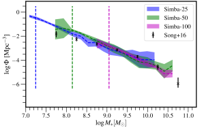
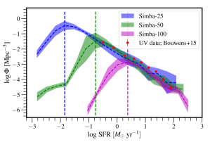
In Figure 1, we show the GSMF and SFR function at $z$  $\sim$ 6. We point out the robust numerical convergence in the GSMF and SFR function (and galaxy properties, see Davé et al. 2019 and §2.2) without refining or fine-tuning the parameters in the sub-grid models of simba between the various simulation boxes at the redshift studied in this work. Note that we do not impose any stellar mass limits in the GSMF plotted. This illustrates the exceptional convergence reached across the boxes. This is crucial as we make predictions of the [CII] LF in the luminosity range of 5.5 $<\log$ ($L_{\rm[CII]}$/$L_{\odot}$) $<$ 8.5 by combining galaxies in the $25\mathrm{cMpc}\,\mathrm{h}^{-1}$, $50\mathrm{cMpc}\,\mathrm{h}^{-1}$, and $100\mathrm{cMpc}\,\mathrm{h}^{-1}$ boxes (hereafter Simba-25, Simba-50, and Simba-100, respectively).

Figure 1.— Top: Galaxy stellar mass function for the different simulation boxes at $z$ = 6 compared to the results based on a rest-frame UV selected observational sample (black markers). Vertical dashed lines show the mass requirement applied to each of the simulation boxes (color-coded) to select only galaxies that are resolved by the simulation (see §2.1). Bottom: Same as the top panel, but for the SFR function. Vertical dashed lines show the thresholds in SFR for each box, below which the boxes become incomplete. The turnover arises from the finite mass resolution of these simulations (before applying the selection criteria; see §2.2). Observational results (corrected for dust attenuation) are plotted as red symbols. The spread marked by the shaded regions is computed from jackknife resampling eight sub-octants of the simulated volumes. Observations are from Song et al. (2016) (top) and Bouwens et al. (2015) (bottom). The simba predictions are in very good agreement with the observational estimates.

2.2. Main Sample: 11,137 Galaxies at $z$ $\simeq$ 6

Galaxies from the simulation suite are identified using a galaxy finder that adopts a 6-dimensional friends-of-friends algorithm (caesar). For the purpose of this work, we include only galaxies that have at least 64 stellar and gas particles, respectively, to ensure they are resolved in the simulation. As illustrated in Figure 1, these mass requirements correspond to $\log{(M_{\rm\star,min}/M_{\odot})}$ = 7.24 for Simba-25, $\log{(M_{\rm\star,min}/M_{\odot})}$ = 8.15 for Simba-50, and $\log{(M_{\rm\star,min}/M_{\odot})}$ = 9.05 for Simba-100. Similarly, we impose thresholds on the SFR averaged over 10 Myr based on the turnover seen in the SFR function indicating incompleteness in SFR. This corresponds to $\log\left(\textrm{SFR}/\textrm{M}_{\odot}\,\textrm{yr}^{-1}\right)>-$1.9, $-$0.8, and $0.4$ for Simba-25, -50, and -100 respectively. In addition, we only include galaxies with a molecular gas mass of at least $M_{\rm mol}$ = $f_{\rm H2}\,M_{\rm gas}$ $>$10⁵ $M_{\odot}$, as the sub-grid model has to form giant molecular clouds (GMCs) of at least 10⁴ $M_{\odot}$ each by sampling the cloud mass from a GMC mass function (see §3). After applying these criteria, we have a sample of $N_{\rm tot}$ = 11,137 galaxies for a single snapshot at $z$  = 6. The ranges of their physical properties are listed in Table 1.

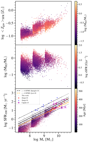
To illustrate the range of physical properties sampled by the simba galaxies, Figure 2 shows the relations between the specific SFR (sSFR), SFR-weighted metallicity ($\langle Z_{\rm gas}\rangle_{\rm SFR}$), molecular gas-to-stellar mass ratio ($M_{\rm mol}$/$M_{*}$), and the stellar mass-weighted age in our $z$ = 6 sample. The three clumps of points represent galaxies from our three simulation volumes, and generally show reasonable convergence. The weighted quantities are indicated with the $\langle...\rangle$ notation (e.g., $\langle Z_{\rm gas}\rangle_{\rm SFR}$), as defined as follows:

$$\langle x\rangle\equiv\frac{\sum_{i}\rho_{i}x_{i}}{\sum_{i}\rho_{i}}\,,$$ (1)

where $x$ is the variable and $\rho_{i}$ is the volume of each fluid element $i$. The $\Sigma_{\rm SFR}$ in this paper is defined as:

$$\Sigma_{\rm SFR}=\frac{\textrm{SFR}}{\pi R_{\rm 1/2}^{2}}$$ (2)

where $R_{\rm 1/2}$ is the half-mass radius of gas of a given galaxy. The scaling relations shown are similar to the mass-metallicity and fundamental metallicity relation (a.k.a. MZR and FMR; e.g., Maiolino et al. 2008; Mannucci et al. 2010), which are commonly used to gain insights into the interplay between star formation, gas accretion, and feedback during the evolution of a galaxy, and are shown to illustrate the range of physical properties sampled by the simba galaxies. As can be seen in the second panel, most of the simba galaxies are rich in molecular gas. The trend of decreasing $M_{\rm mol}/$$M_{*}$ with increasing $M_{*}$ arises owing to stellar feedback which preferentially suppresses the stellar mass in lower mass systems, thereby increasing $M_{\rm mol}$/$M_{*}$. The middle panel also shows how, for a given stellar mass bin, the SFR increases with the molecular gas mass fraction, as expected. That said, there are certainly jumps in $M_{\rm mol}/$$M_{*}$ fractions between the different simulations volumes indicating less than ideal convergence, although this becomes less apparent when plotting $M_{\rm mol}$ against $M_{*}$ as shown in the left panel of Fig. 12 in the Appendix. The bottom panel displays the simba galaxies on top of the “star-forming main sequence” (SFMS; e.g., Speagle et al. 2014; Iyer et al. 2018), which most of our galaxies follow at $\log M_{*}\gtrsim 9$ $M_{\odot}$— which is also the stellar mass limit of the observational data. At lower stellar mass, the sSFR of simba galaxies falls below the SFMS extrapolation. The color coding in the three panels shows that, at a given stellar mass, galaxies that are higher metallicity have lower gas contents, galaxies that have higher gas contents have higher sSFR, and galaxies that have higher sSFR have lower mean stellar age.

Galaxies of similar stellar masses and SFRs may have different sizes, surface densities, gas contents, metallicities, interstellar radiation field strengths, structural properties, and gas dynamics; all of which would produce varying [CII] luminosities (see e.g., Kaufman et al. 1999; Vallini et al. 2015; Olsen et al. 2017). As such, comparing the physical properties of observed (i.e., [CII]-detected ones in the context of this work) and simulated galaxies is pertinent to establishing the reliability of model predictions. In other words, comparing these global properties of simba galaxies with those of observed galaxies enables one to place the observed ones, given their [CII] luminosities, in a theoretical framework. It is beyond the scope of this paper to perform a detailed comparative study since the information available for observed galaxies at these redshifts (see §4.1) remains limited and inhomogeneous. For comparisons of simba galaxies with observations at lower redshifts and discussion on redshift evolution in these relations, we refer interested readers to Davé et al. (2019). At the EoR, the size-luminosity relation of simba galaxies agrees with observations (Kawamata et al. 2018; Wu et al. 2019).

Figure 2.— Scaling relations for the simba galaxy sample (circular dots). Top: $\langle Z_{\rm gas}\rangle_{\rm SFR}$ – $M_{*}$ relation, color-coded by the molecular gas mass fraction. Middle: Molecular gas-to-stellar mass ratio ($M_{\rm H2}$/$M_{*}$) – $M_{*}$ relation, color-coded by sSFR. Bottom: SFR–$M_{*}$ relation, color-coded by the mass-weighted stellar age. The SFR of the simulated galaxies are averaged over 100 Myr. Magenta squares, red crosses, and blue plus symbols correspond to observations of UV-selected star-forming galaxies at $z$ $\sim$ 6 (Capak et al. 2015; Jiang et al. 2016), with the red markers indicating older galaxies with a crude estimated age of $\gtrsim$ 100 Myr and the blue ones indicating younger galaxies with age $\lesssim$ 30 Myr. Dashed lines correspond to empirical relations for the star-forming main sequence (SFMS) and their 1$\sigma$ and 3$\sigma$ spreads at this redshift (Speagle et al. 2014; Iyer et al. 2018). The sharp cutoffs seen in the last two plots results from the mass cut imposed on each of the simulation boxes (Simba-25, Simba-50, and Simba-100) to only include galaxies that are numerically resolved (see §2.2).

Table 1Parameter space probed by our simba galaxy sample at $z$ $\sim$ 6.

Properties	Units	Ranges
$\log M_{\rm halo}$	$M_{\odot}$	[9.02 12.36]
SFR10	$M_{\odot}$  yr-1	[0.01, 708]
SFR100	$M_{\odot}$  yr-1	[0.007, 329]
$\log\Sigma_{\rm SFR}$	$M_{\odot}$  yr-1  kpc-2	[-2.60, 1.31]
$\log$ $M_{*}$	$M_{\odot}$	[7.18, 10.72]
$\log$ $M_{\rm gas}$	$M_{\odot}$	[7.27, 10.46]
$\langle Z_{\rm gas}\rangle_{\rm SFR}$	$Z_{\odot}$	[0.06, 1.86]

3. Method: Simulating Line Emission

We use an updated version of sígame (Olsen et al. 2015, 2017) to post-process the simba simulation outputs. For details of the code, we refer interested readers to Olsen et al. (2017). Here, we briefly summarize the salient points of sígame and updates made to the code as part of this work. For each gas fluid element, sígame divides the molecular gas mass (i.e., $f_{\rm H2,i}\,m_{\rm gas,i}$) into GMC by sampling the Galactic GMC mass function over the mass range of 10^4-6 $M_{\odot}$ ($dn/dM\propto M_{\rm GMC}^{-1.8}$; see e.g., the review by McKee & Ostriker 2007; Blitz et al. 2007; Kennicutt & Evans 2012). The remaining mass of the parent fluid element is assumed to be in the diffuse gas phase, and is subsequently distributed into diffuse ionized and neutral gas phases. This division is determined by the boundary at which the inner neutral region transitions to the outer ionized region of the diffuse clouds as computed from RT calculations within Cloudy. That is, the neutral gas phase corresponds to the region beyond a radius where the neutral fraction $x_{\rm HI}=n_{\rm HI}/(n_{\rm HI}+n_{\rm HII})>\,$0.5, such that it is dominated by neutral hydrogen — here $n$ is the number density. As such, sígame accounts for line emission from three distinct ISM phases. The smoothing length of the parent fluid element is adopted as the size of the diffuse gas clouds, whereas the size of each GMC is derived from a pressure-normalized mass-size relation, following

$$\frac{R_{\rm GMC}}{\rm pc}=\left(\frac{P_{\rm ext}/k_{\rm B}}{10^{4}\,{\rm cm}^{-3}\,{\rm K}}\right)^{-1/4}\left(\frac{M_{\rm GMC}}{290~{}M_{\odot}}\right)^{1/2},$$ (3)

where $k_{\rm B}$ is the Boltzmann constant and the external cloud pressure $P_{\rm ext}$ is defined assuming mid-plane hydrostatic equilibrium within the galaxy.

Each GMC radial density profile is assumed to follow a truncated logotropic profile. Both GMCs and diffuse gas phases inherit the metallicity of their parent fluid element. The FUV luminosity of each star is calculated based on its age and metallicity and is determined by interpolating over a grid of starburst99 stellar population synthesis models (Leitherer et al. 2014) (with the default Kroupa 2002 initial mass function). Each GMC is irradiated by a local FUV radiation (6–13.6 eV), where the strength of the radiation field ($G_{0}$ in Habing units; 1.6$\times 10^{-3}$ erg cm^-2 s ^-1) is determined by summing up the FUV flux from nearby stellar particles and by assuming that the flux falls off as $1/r^{2}$. In the diffuse gas phase, the FUV radiation field is determined based on the SFR surface density of the galaxy. For our sample, the SFR surface density ranges between $\simeq$ 1 – 6200 times the Milky Way.

We use the photoionzation code cloudy version 17.01 (Ferland et al. 2017) to simulate the thermo-chemistry in the three distinct ISM phases tracked by sígame by performing detailed balance calculations of the various species, taking into account physical processes such as H₂ photo processes, dust physics (grain-atom/ion charge transfer), and cosmic ray (CR) ionization. The line luminosities are then derived from the cooling rates for different line transitions. For computational purposes, lookup tables are generated for the GMC and the diffuse (neutral and ionized) gas phase, respectively. The FUV radiation field impinging on the gas phases is assumed to have the same spectral shape as in the solar neighborhood.

Cosmic rays are added, with an ionization rate equal to that of the Milky Way scaled linearly by a factor of $(G_{0,\rm gas}/G_{0,\rm MW})$. For the GMC models, the clouds are in theory completely embedded within diffuse gas, and thus H-ionizing radiation is turned off in the Cloudy models (cf. Olsen et al. 2017).

The main parameters in the GMC phase of the cloudy models considered are the $G_{\rm 0,GMC}$ of the radiation source, radius of the cloud ($R_{\rm GMC}$), and cloud density profile as a function of cloud radius ($n_{H}(R_{\rm GMC})$). Turbulent velocity is added to the GMC models according to the velocity dispersion calculated from the cloud radius and pressure, assuming clouds are virialized. For the diffuse gas phase, the main model parameters are gas density ($n_{H}$), gas kinetic temperature ($T_{k}$), diffuse cloud size, ($R_{\rm dif}$), and metallicity ($Z$).

Compared to Olsen et al. (2017), the main updates made to sígame used in this work are as follows:

• Instead of fixing the number and width of shells used by cloudy to model each GMC, we now allow cloudy to determine the optimal quantities to ensure convergence. This modification leads to more accurate calculation of the grain photoelectric heating of the gas and increases the importance of gas heating due to this mechanism in the GMC models, which is the main excitation mechanism for [CII] emission. Namely, [CII] is collisionally excited such that higher kinetic temperature leads to more molecular motions and collisions inside GMCs and photo-dissociation regions (PDRs), the main sites for [CII] emission in galaxies.

• To ensure good sampling of the parameter space for both GMCs and diffuse gas clouds, the number of cloudy models used to create look-up tables is significantly increased from 1296 to 4096 models by using 8 grid points in each parameter space dimension rather than 6 as in Olsen et al. (2017). The look-up tables are further described in §3.1.

• The dust content of the ISM is a crucial factor in setting the [CII] luminosity. As often done, we will assume here that dust scales with metallicity via the dust to metal ratio (DTM), but instead of using a solar DTM value of $\sim 0.46$ (as done in Olsen et al. (2017)), we take a DTM of 0.25 based on the mean value of our simba galaxies (see §3.1).

3.1. GMCs and Diffuse Gas Phase Properties and cloudy Model Grids

As mentioned in the previous section, the parameters passed to cloudy for GMCs and diffuse gas clouds are; $M_{\rm GMC}$, $G_{\rm 0,GMC}$, $Z$, and $P_{\rm ext}$ for the GMC models and in $n_{H}$, $T_{k}$, $R_{\rm dif}$, and $Z$ for diffuse gas models.

For the GMCs, we generate 4096 models spanning $\log(M_{\rm GMC}/M_{\odot})\in$[4.1, 4.3, 4.6, 4.8, 5.1, 5.3, 5.6, 5.8], $\log(G_{\rm 0,GMC}/G_{\rm 0,MW})\in[$0.3, 1.0, 1.6, 2.3, 3.0, 3.7, 4.3, 5.0], $\log(Z/Z_{\odot})\in[-$3, $-$2.5, $-$2.1, $-$1.6, $-$1.2, $-$0.7, $-$0.3, 0.2], and $\log(P_{\rm ext}/k_{B})\in[$4.0, 4.9, 5.7, 6.6, 7.4, 8.3, 9.1, 10.0] cm^-3 K. For the diffuse gas, we first determine the SFR surface density of all the galaxies of the sample. We then define a range of FUV grids over $(G_{\rm 0,GMC}/G_{\rm 0,MW})\in$[0.8, 7.2, 68, 650, 6200] based on the ranges of SFR surface densities found in the simulated galaxies as a hyperparameter. For each of the FUV grid, we generate 4096 models spanning $\log(n_{H}/{\rm cm}^{3})\in$[$-$5.0, $-$4.32, $-$3.66, $-$2.99, $-$2.31, $-$1.64, $-$0.97, $-$0.3], $\log(T_{k}/{\rm K})\in$[2.5, 3.0, 3.6, 4.2, 4.8, 5.4, 5.9, 6.5], $\log(R_{\rm dif}/{\rm kpc})\in$[$-$0.7, $-$0.49, $-$0.27, $-$0.06, 0.16, 0.37, 0.59, 0.8], and $\log(Z/Z_{\odot})\in[-$1.0, $-$0.83, $-$0.66, $-$0.49, $-$0.31, $-$0.14, 0.03, 0.2].

The gas kinetic temperature in the GMC phase is left as a free parameter to be determined by solving the thermal balance equation in cloudy, whereas in the diffuse gas phase, the temperature is fixed to the grid points representative of the range seen in the gas fluid elements from the simba simulation. The effect of gas heating due to the photo-excitation by the cosmic microwave background (CMB) at the EoR is included. The resulting line intensities are corrected to give the net flux above the background continuum (i.e., not the contrasting flux that observers would measure; see e.g., da Cunha et al. 2013), and include the diminution effect where the upper levels are sustained by CMB (Ferland et al. 2017).

3.2. Dust and Elemental Abundances

While simba tracks dust in the simulation, we do not create a different cloudy lookup table for each dust-to-mass (DTM) ratio found in the simulated galaxies since this becomes computationally intractable (i.e., it corresponds to a hyperparameter where each DTM ratio would have a separate set of 4096 cloudy models). Instead, we adopt a DTM ratio based on the median of simba galaxies at $z\sim 6$, corresponding to $\xi_{\rm DTM}$ = 0.25, which is defined as

$$\xi_{\rm DTM}=\frac{M_{\rm dust}}{f_{Z}~{}M_{\rm gas}+M_{\rm dust}},$$ (4)

where $M_{\rm dust}$ and $M_{\rm gas}$ are the dust mass and total gas mass in solar mass units, and $f_{Z}$ is the mass fraction of metals (i.e., $f_{Z}~{}M_{\rm gas}$ yields the mass of metals in gas-phase). The dust content of each cloud is then set to scale linearly with its metallicity through this DTM. The default set of lookup tables in Cloudy assumes a DTM of $\xi_{\rm DTM}$ = 0.46 at solar metallicity. A more commonly adopted expression for the DTM is:

$$\textrm{DTM}\equiv\frac{\textrm{DGR}}{\textrm{Z}}.$$ (5)

In the Milky Way, Z = $Z_{\odot}$ and DGR is $\sim$0.01, yielding $\log$ DTM = $-$2.

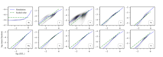
In cloudy, one can supply the total metallicity, and the abundance of each of the elements is scaled correspondingly assuming Solar composition (i.e., abundance ratios of the Sun). In order to account for abundance patterns of galaxies that differ from Solar, we use the abundance of each metal tracked in simba (i.e., He, C, N, O, Ne, Mg, Si, S, Ca, and Fe). For elements that are not tracked in the simulation, we use Solar abundance ratios. Since the mass fraction of each element tracked varies as a function of metallicity, we fit a spline curve to the running means across all gas fluid elements. This provides a function that maps a given metallicity to an abundance pattern, such that the relative elemental abundances in the cloudy input are scaled according to the metallicity of the cloud. In the Appendix we show the particle distribution and scalings found for our sample of simba galaxies. We note that some elements, like carbon and nitrogen, can be quite far from their solar abundance value, which in simba is a result of including enrichment from Type II supernovae (SNe), Type Ia SNe, and Asymptotic Giant Branch (AGB) stars, with separate yield tables for each class of star as described in Oppenheimer & Davé (2006).

4. Results and Discussion

4.1. [CII]– SFR Relation at $z$ $\simeq$ 6

Figure 3.— SFR and $L_{\rm[CII]}$ of simba galaxies at $z$  = 6 (hexbin) compared to existing observations and models at the EoR. Red lines show the running mean and standard deviations of the binned data for simba galaxies. Results from a sample of 30 (zoom-in) mufasa galaxies at $z$ $\simeq$ 6 are shown as green shaded regions (Olsen et al. 2017), whereas those from SAM-based predictions at $z$  = 6 are shown as light red shaded regions (Popping et al. 2019), and results from zoom-in AMR simulations from Pallottini et al. (2017b) and Pallottini et al. (2017a) are shown as blue stars. Fits to observations from $z$  = 0 are shown as gray and blue shaded regions (De Looze et al. 2014; Herrera-Camus et al. 2015). Square symbols show observations at $z\simeq$6 compiled from Ouchi et al. (2013); Kanekar et al. (2013); Ota et al. (2014); González-López et al. (2014); Maiolino et al. (2015); Schaerer et al. (2015); Capak et al. (2015); Willott et al. (2015); Bradač et al. (2017); Inoue et al. (2016); Pentericci et al. (2016); Knudsen et al. (2016, 2017); Decarli et al. (2017); Smit et al. (2017); Carniani et al. (2018b) and Uzgil et al. 2020, in prep.

Figure 4.— Same as Figure 3, but visualized across three panels for clarity. Top: Running mean and standard deviations of $z$ = 6 simba galaxies (red) overplotted with $z$ = 0 observations. The predicted $L_{\rm[CII]}$/SFR for galaxies with SFR $\gtrsim 1$ are 1-2 dex lower than observed galaxies in the local Universe, and the slope of the $L_{\rm[CII]}$ vs. SFR relation is shallower. Middle: simba galaxies (red line) overplotted with other $z$ = 6 models in the literature (see legend). Our model predictions are in reasonable agreement with those of other studies, especially at higher SFR, but we predict a shallower $L_{\rm[CII]}$ vs. SFR relation than other studies. Bottom: simba galaxies (red line and hexbin) overplotted with $z$ = 6 observations. The hexbins are color-coded by the density of points, see Figure 3 for colorbar. Our predictions show reasonable overlap with the locus of the heterogeneous observational samples, although we do not produce any galaxies with $L_{\rm[CII]}$ values as high as those of some of the detected galaxies at high SFR $\gtrsim 10$. See text for a discussion of possible reasons for these discrepancies.

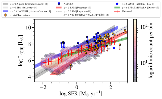
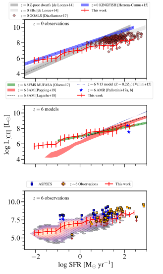
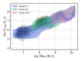
In Figure 3, we plot the simulated $L_{\rm[CII]}$ and SFR of the simba galaxies together with measurements from existing observations at $z\,\simeq$ 6, local measurements, and other model predictions at $z\,\simeq$ 6. The $L_{\rm[CII]}$-SFR relation converges across the different simulation volumes as does the $L_{\rm[CII]}$-$M_{\rm mol}$ relation as seen in the right panel Fig. 12 in the Appendix. For clarity, information shown in this figure is also plotted across three panels in Figure 4. We fit a linear model to $L_{\rm[CII]}$ and SFR in log-log space to facilitate comparison with literature work, and obtain

$$\log L_{\rm[CII]}=(6.82\pm 0.08)+(0.66\pm 0.01)\times\log{\rm SFR},$$ (6)

where $L_{\rm[CII]}$ is in units of $L_{\odot}$, and SFR is in units of $M_{\odot}$  yr^-1.

The [CII] luminosities of the simba galaxies are consistent with existing upper limits and a handful of detections from targeted observations (e.g., Ouchi et al. 2013; Kanekar et al. 2013; Ota et al. 2014; González-López et al. 2014; Maiolino et al. 2015; Schaerer et al. 2015; Capak et al. 2015; Willott et al. 2015; Inoue et al. 2016; Pentericci et al. 2016; Knudsen et al. 2016; Inoue et al. 2016; Bradač et al. 2017; Knudsen et al. 2017; Decarli et al. 2017; Smit et al. 2017; Carniani et al. 2018b). In addition, our results are in agreement with the latest upper limits placed at $z\simeq\,$6 by the ALMA large program ASPECS, which is an untargeted survey, placing an upper limit of $L_{\rm[CII]}$ $<$ 2$\times 10^{8}$ $L_{\odot}$ for galaxies with UV-derived SFR of $\sim$ 0.25–50 $M_{\odot}$  yr^-1 (Walter et al. 2016, Uzgil et al., in prep.). In particular, the ASPECS sources with upper limits on $L_{\rm[CII]}$ shown in Figure 3 with blue squares are a combination of Lyman-$\alpha$ emitters (LAEs) with spectroscopic redshifts from the MUSE survey (Inami et al. 2017), and Lyman break galaxies (LBGs) (Bouwens et al. 2015). The Lyman-$\alpha$ luminosities of the LAEs are L_Lyα = 0.7 $-$ 1.5$\times 10^{42}$ erg s^-1, with UV-based SFR $<$ 4 $M_{\odot}$  yr^-1, and stellar mass of $\log(M_{*}/M_{\odot})$ = 8.04 – 8.75 (note that only two of the six MUSE LAEs have stellar mass constraints). The LBGs have H-band magnitudes of H₁₆₀ = 27.5–30.9 mag, corresponding to a UV-based SFR of 0.25 – 48 $M_{\odot}$  yr^-1, and have stellar masses between $\log(M_{*}/M_{\odot})$ = 7.99 – 9.37. In general, the running mean in [CII] luminosity of the simba sample is lower than the average of existing detections of targeted observations at $z$ $\sim$ 6.

Our results are consistent with those based on the Serra simulation suite by Pallottini et al. (2017b) and Pallottini et al. (2017a), which is a suite of cosmological zoom-in AMR simulations that resolve the gas down to 10 pc-scales at $z\simeq$ 6. It is also in reasonably good agreement with the sample of 30 mufasa galaxies analyzed in Olsen et al. (2017), thus broadly confirming these results using a larger sample from its successor simulation (simba), while reaching comparable resolution over cosmological volumes. That said, our results yield a flatter $L_{\rm[CII]}$–SFR relation than other models at $z\,\simeq$ 6, such as those based on SAMs and semi-empirical models (Vallini et al. 2015; Lagache et al. 2018; Popping et al. 2019). We discuss the potential causes of the differences seen between our results and other models in the literature in §5.

4.2. [CII] Luminosity Function at $z$ $\simeq$ 6

Figure 5.— [CII] LF predicted at $z$ $\simeq$ 6 based on the cosmological hydrodynamics simulation simba. Shaded regions are obtained by jackknife resampling of the simulation sub-volumes. The flattening and turnover at the faintest end is due to incompleteness of haloes with $\log$ $L_{\rm[CII]}$ $\lesssim$ 6 $L_{\odot}$. Results from SAM-based models are overplotted as dashed lines (Popping et al. 2016, 2019). Our results are fully consistent with the SAM-based model predictions within the error bars and the upper limits from ASPECS (blue symbol; Uzgil et al., in prep.).

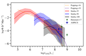
In Figure 5, we show predictions for the [CII] LF at $z$ $\simeq\,$6 based on the simulated $L_{\rm[CII]}$ of galaxies in Simba-25, Simba-50, and Simba-100. We note that previously, LF predictions were only possible in models that made more simplified assumptions to connect $L_{\rm[CII]}$ to dark matter halos. Nonetheless, our results are in agreement with those based on SAMs by Lagache et al. (2018) and Popping et al. (2019), and with constraints from the latest limits placed using data from ASPECS (Uzgil et al., in prep.; see footnote 3).

Using the Capak et al. (2015) targeted sample, Hemmati et al. (2017) report a volume density that is almost an order of magnitude higher than our results at the bright end at $\log$ $L_{\rm[CII]}$ $\gtrsim$ 8.5 $L_{\odot}$, although they are consistent within the error bars. Note that the actual uncertainties on the [CII] LF constrained by the Capak et al. (2015) sample are likely to be larger than those reported by Hemmati et al. (2017), as incompleteness and selection bias are not corrected for. As shown in Figure 3, most of the simba galaxies have $L_{\rm[CII]}$  = 10^6-8 $L_{\odot}$. Thus, it is unsurprising to see a discrepancy in the [CII] LF between the Capak et al. (2015) sample and our sample due to the lack of overlap in terms of $L_{\rm[CII]}$.

Miller et al. (2016) derive a [CII] LF using the Bolshoi-Planck dark matter only simulation catalog from Behroozi et al. (2013), the abundance matched SFR from Hayward et al. (2013), and the empirical $L_{\rm[CII]}$–SFR relations established at $z$ $\sim$ 0 by De Looze et al. (2014). Consistent with our results, Miller et al. (2016) report a [CII] LF that underpredicts the observational constraints placed by Hemmati et al. (2017) using the Capak et al. (2015) sample and that placed based on a blind search of five deep fields centered on IR-bright galaxies and quasar host galaxies at $z$ $\sim$ 6. By simulating only regions with $L_{\rm[CII]}$ matched to the central galaxies observed in the deep fields (8.7 $<\,\log$$L_{\rm[CII]}$/$L_{\odot}$ $<$ 9), Miller et al. (2016) find a good agreement between the [CII] LF and the observational constraints. On this basis, they argue that the [CII]-detected sources in the deep fields are indeed in biased overdense regions. This may partially explain the discrepancy seen between the observed and the simba based [CII] LF — since the largest simulation box of simba is 100 cMpc, and it may not contain these rare highly biased regions.

4.3. $L_{\rm[CII]}$  – M_halo Relation

Forecasts for upcoming [CII] LIM surveys have been obtained using scaling relations between [CII] luminosity and halo mass, where the latter quantity is obtained from large volume N-body simulations (e.g., Silva et al. 2015; Kovetz et al. 2017). The large cosmological volumes provided by N-body simulations are needed to make mock lightcones for LIM (e.g. Yang et al. 2020); however, most previous work in this area has made simple empirical assumptions regarding the relationship between dark matter halo properties and [CII] line luminosity. Here we study the $L_{\rm[CII]}$  – M_halo relation based on the central galaxies in our cosmological hydrodynamic simulation.

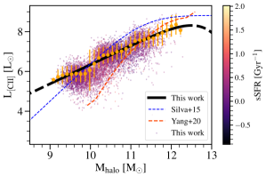
In Figure 6, simba galaxies are shown in $L_{\rm[CII]}$ versus M_halo with a fit made following the formalism of Silva et al. (2015), where SFR is expressed in terms of M_halo:

$${\rm SFR}=M_{0}\times\left(\frac{M_{\rm halo}}{M_{a}}\right)^{a}\left(1+\frac{M_{\rm halo}}{M_{b}}\right)^{b}.$$ (7)

Together with the expected linear relation between $L_{\rm[CII]}$ and SFR, the following equation relates M_halo to $L_{\rm[CII]}$:

$$\log L_{\rm[CII]}=M^{\prime}_{0}+a^{\prime}\log\left(\frac{M_{\rm halo}}{M^{\prime}_{a}}\right)+b^{\prime}\log\left(1+\frac{M_{\rm halo}}{M^{\prime}_{b}}\right),$$ (8)

where $L_{\rm[CII]}$ is in units of $L_{\odot}$, and M_halo is in units of $M_{\odot}$. With the current set of parameters adopted in the sub-grid model (see §3), the fitted parameters are $a^{\prime}$ = 0.65, $b^{\prime}$ = $-$9.85, $M^{\prime}_{0}$ = 3.62, $M^{\prime}_{a}$ = 1.50$\times 10^{7}$, and $M^{\prime}_{b}$ = 2.90$\times 10^{13}$.

The $L_{\rm[CII]}$– M_halo relation of central galaxies in simba has a scatter of $\simeq$ 0.5 dex around the fit. We also show the running mean in the same figure which follows the parametric form. In the same figure, we show a comparison with the $L_{\rm[CII]}$– M_halo relation from a SAM (Popping et al. 2019; Yang et al. 2020), which is steeper than both Silva et al. (2015) and this work; but is however, consistent within the scatter of simba galaxies.

Figure 6.— $L_{\rm[CII]}$ $-$ M_halo of simba galaxies studied in this work, color-coded by sSFR (dot symbols). The black line shows the best-fit parametric model, whereas the orange dots show the mean when the simba data is binned in 30 logarithmic intervals in M_halo (i.e., non-parametric). The blue dashed line shows the m1 model of Silva et al. (2015) at a comparable redshift. The red line shows the model from Yang et al. (2020) based on SAMs by Popping et al. (2019). Although there is qualitative agreement between the different models, the remaining discrepancies could have significant implications for predictions for upcoming line intensity mapping surveys.

5. Discussion: Discrepancies and Caveats

Table 2Quick comparison of approaches between existing models in simulating [CII] emission at $z$ $\sim$ 6.

	Vallini15	Olsen17	Pallottini17a,b	Lagache18	Popping19	This work
Simulation technique	SPH	MFM	AMR	SAM	SAM	MFM
Gas mass/cell resolution ($M_{\odot}$)	105.1	105.3	104.1	—	—	105.5-7.3
Min. gravitational softening length ($h$-1 kpc)	—	0.01	—	—	—	0.125–0.5
Stellar emission calculation	Licorice, starburst99	starburst99	starburst99	BC03	scaled by SFR volumetric density	starburst99
Line emissivity calculation	ucl_pdr	cloudy	cloudy	cloudy (PDR only)	despotic	cloudy
Number of Galaxies	1	30	2	25,000	$>$230,000	11,137

Note. — Literature models from Vallini et al. (2015); Olsen et al. (2017); Pallottini et al. (2017b, a); Lagache et al. (2018); Popping et al. (2019).

As discussed in §4, our predicted [CII] LF is consistent with that predicted from other models based on SAMs, and the simba galaxies lie in the same region of $L_{\rm[CII]}$– SFR as the galaxies studied by one of the most detailed cosmological zoom-in AMR simulations at the same redshift (Pallottini et al. 2017b, a). However, compared to other models, our model underpredicts the [CII] luminosity at the bright end (and high SFR; Figure 4) and yields a flatter $L_{\rm[CII]}$– SFR relation. This discrepancy may arise from for instance different ranges of properties for galaxies in the samples, different predicted scaling relations between galaxy properties in different galaxy evolution models, a limited number of massive halos in our simulation, and the different sub-grid treatments of physical processes in simba and in sígame compared to other approaches adopted in the literature used for comparison here (Table 2). For instance, Vallini et al. (2015) simulate the [CII] line emission by post-processing the UV radiation field of an SPH-based simulated galaxy using Licorice, and calculate the [CII] emission using a combination of an analytical model and the photo-dissociation region (PDR) code ucl_pdr (Bayet et al. 2009 and references therein; to account for contributions from PDR). While the sub-grid modeling of Popping et al. (2019) follows a similar approach as sígame, the former is based on a SAM while the latter is applied to hydrodynamical simulations. As a result, there are relatively subtle differences between the two, such as the assumption of exponential gas disks for all galaxies in the former. In addition, the former approach assumes that all GMCs in each galaxy share the same metallicity based on the global metallicity, and adopts despotic instead of cloudy in performing the thermochemistry calculation. As mentioned in §1, despotic does not account for line emission in the ionized phase while the latter does. In contrast to Popping et al. (2019), Lagache et al. (2018) use cloudy to post-process their SAM. While using cloudy is the same approach as sígame (including this work) and works by e.g., Katz et al. (2019) and Pallottini et al. (2019), Lagache et al. (2018) adopt different sub-grid approaches and assumptions compared to those made for hydrodynamical simulations. In particular, their model does not account for [CII] emission coming from regions outside of PDRs, the complexity of the multiphase ISM, and the detailed structures of molecular clouds. This illustrates the various differences between existing models which can contribute to the discrepant $L_{\rm[CII]}$– SFR slopes. Using SAMs, Popping et al. (2019) experiment with different assumptions made in the sub-grid approaches and indeed find differences in the resulting [CII] luminosity.

Lagache et al. (2018) report that after selecting galaxies with the same range of stellar mass, SFR, and gas-phase metallicities as the Mufasa sample studied by Olsen et al. (2017) — i.e., with $M_{*}\in$ (0.7–8)$\times 10^{9}$ $M_{\odot}$, SFR$\in[$3–23$]$ $M_{\odot}$  yr^-1, and $Z_{\rm gas}\in[$0.15–0.45$]$ $Z_{\odot}$ — the $L_{\rm[CII]}$– SFR relation of their SAM galaxies is flatter and more consistent with that of Olsen et al. (2017). Yet, this relation remains flatter than that obtained when applying the same set of criteria to the SAM galaxies of Popping et al. (2019) (9,653 galaxies after selection). In Figure 7, we show the $L_{\rm[CII]}$– SFR for a subset of simba galaxies selected based on these criteria (1,136 galaxies) compared to Olsen et al. (2017) and Popping et al. (2019). A relation with a flatter slope than Popping et al. (2019)’s SAM-based models persists for the simba galaxies.

Figure 7.— Region of $L_{\rm[CII]}$– SFR in log-space spanned by simba galaxies (teal line) and galaxies from Popping et al. (2019; magenta line) selected with the same range in stellar mass, SFR, and gas-phase metallicities as Olsen et al. (2017) (green shaded). A relation with a flatter slope than other models persists for the simba galaxies (see §5).

Figure 8.— Normalized distributions of stellar mass, SFR, molecular gas mass, and metallicity between the subset of galaxies from Popping et al. (2019) (blue) and this work (green) after applying the Olsen et al. (2017) selection. While distributions in SFR are comparable, the subset of galaxies from the Popping et al. (2019) sample have higher molecular gas mass and metallicity compared to the simba subset.

Figure 9.— Distributions of $L_{\rm[CII]}$ across all simba galaxies, in the first (red) and third (cyan) quartiles in molecular gas mass from different SFR bins (second through last panels). See text for the SFR covered by each bin. The top panel shows the distributions across all SFR. At a fixed SFR, galaxies with higher $M_{\rm mol}$ have higher $L_{\rm[CII]}$.

Figure 10.— Same as Figure 9 but for metallicity. At a fixed SFR, galaxies with higher $\langle Z_{\rm gas}\rangle_{\rm SFR}$ have higher $L_{\rm[CII]}$.

Figure 11.— Same as Figure 9 but for SFR surface density. Overall, galaxies with higher $\Sigma_{\rm SFR}$ have higher $L_{\rm[CII]}$, but this trend is not seen after accounting for the influence caused by different SFR.

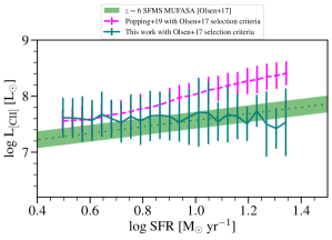
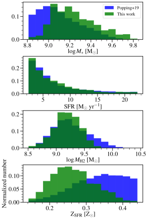
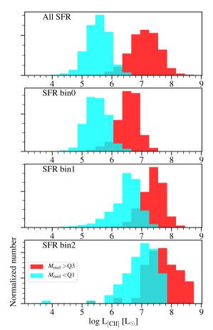
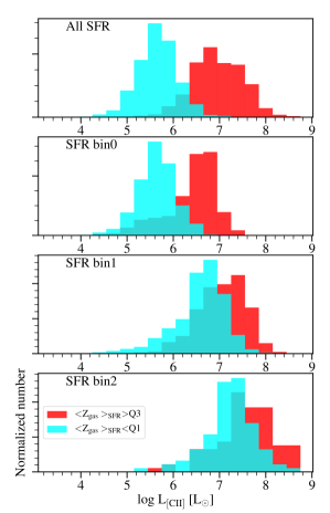
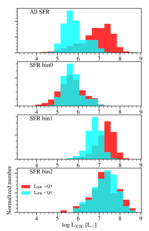
As shown and discussed in the literature (e.g., Vallini et al. 2015; Olsen et al. 2017; Lagache et al. 2018; Pallottini et al. 2019; Popping et al. 2019), a lower metallicity can result in a lower $L_{\rm[CII]}$ at given SFR. In fact, as shown in Figure 8, while the distributions in SFR between the subset of galaxies from the Popping et al. (2019) sample and this work are comparable after applying the Olsen et al. (2017) selection cut, the former are more metal rich, with higher molecular gas masses compared to the latter. The trend of decreasing molecular gas mass and metallicity with $L_{\rm[CII]}$ is also seen in Figures 9 and 10, where we show the different $L_{\rm[CII]}$ distributions when the full set of 11,137 simba galaxies are selected using the first and third quartiles in molecular gas mass and metallicity, respectively. To account for the effect of SFR in $L_{\rm[CII]}$, we bin the galaxies into three SFR bins, $\in[0.01,10.3]$, $\in[0.3,10.3]$, $\in[10.3,329]$ $M_{\odot}$  yr^-1 . At least in the lowest SFR bin, the variation seen in the [CII] luminosity is mostly driven by the lower metallicity and molecular gas mass (see also Narayanan & Krumholz 2017). Across all SFR, galaxies with lower $L_{\rm[CII]}$ correspond to those with the least molecular gas mass, metallicity, and SFR surface density (Figures 9, 10, and 11).

As mentioned in §1, models in the literature adopt different approaches and assumptions in post-processing the simulations. This could also yield different simulated line luminosities. A steeper slope, more compatible with other models in the literature, namely Vallini et al. (2015) and Popping et al. (2019), would result from adopting the local ISM abundance ratios instead of the abundance pattern tracked in simba (see §3.2 and Olsen et al. 2017). Both Vallini et al. (2015) and Popping et al. (2019) adopt a Solar abundance pattern (of relevance to this work is the C/H ratio) and scale the C/H ratio according to the gas-phase metallicity of each galaxy to determine the [CII] emissivity. That is, their models do not consider abundance patterns that differ from Solar. The resulting $L_{\rm[CII]}$ could differ significantly owing to the amount of cooling via C⁺. On the other hand, Lagache et al. (2018) accounted for abundance ratios that differ from Solar. Specifically, they scale the element abundances based on the median of their sample. Unsurprisingly, the slopes of the $L_{\rm[CII]}$– SFR relation of mufasa and simba galaxies are the most compatible to the Lagache et al. (2018) model. As mentioned by Lagache et al. (2018) and Katz et al. (2019), details in modeling the interstellar radiation field intensity, self-shielding, and the choice and implementation of stellar feedback are all effects that can cause differences between existing models (see also Pallottini et al. 2017b).

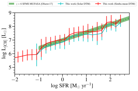
In contrast to mufasa, where dust is not tracked in the simulation, causing Olsen et al. (2017) to adopt a constant DTM ratio, simba tracks dust in the simulation; however, we do not create a different cloudy lookup table for each DTM ratio since it would become computationally intractable. The mean DTM of simba galaxies is $\xi_{\rm DTM}$ = 0.25, which yields a [CII] luminosity approximately $\lesssim$ 0.5 dex higher than for models with a DTM ratio set to the Solar value of $\xi_{\rm DTM}$ = 0.46 (see Appendix; cf. Olsen et al. 2017 who finds that $L_{\rm[CII]}$ only increased by $\sim 0.15$  dex at a given SFR when decreasing the DTM by a factor 2 from Solar DTM for their Mufasa SFMS sample). Note that in reality, the DTM ratio varies from galaxy to galaxy (and within galaxies themselves), and is correlated with the galaxy metallicity (e.g., Rémy-Ruyer et al. 2014; Popping et al. 2017; De Vis et al. 2019). Since the standard deviation of the DTM ratio of the simba sample studied here is $\sigma$ $\sim$ 0.15, we do not expect the simulated [CII] luminosity to deviate more than 0.5 dex as a result of variations in the DTM ratio.

A final important caveat is that the effect of AGN was not included in the present modeling with cloudy, although cloudy does have the capability to do so and this has been shown to be relevant at least for CO line emission at high redshift (Vallini et al. 2019), and hence likely also relevant for [CII]. The effect of AGN is an additional feature that we wish to include in the future.

6. Summary and Conclusions

In this work, we presented the first prediction of the [CII] luminosity function (LF) during the Epoch of Reionization (EoR; $z\simeq$ 6) based on large-volume cosmological hydrodynamical simulations (simba) coupled with radiative transfer and line spectral synthesis calculations. We simulate the [CII] line luminosity for a sample of 11,137 galaxies identified in the combined 25, 50, and 100 $\mathrm{cMpc}\,\mathrm{h}^{-1}$ boxes (with 2 $\times$ 1024³ particles each) at $z\simeq$ 6. The runs for the three simulation boxes have identical input physics, and produce converged GSMF and SFR functions without fine-tuning the parameters in the sub-grid models of simba. In addition, both GSMF and SFR functions are in good agreement with observations at this redshift. This is crucial as we make predictions for the [CII] LF in the luminosity range of 5.5 $<$ $\log$($L_{\rm[CII]}$/$L_{\odot}$)$<$ 8.5 by combining the boxes.

We use an updated version of sígame to post-process the simba output. Three major improvements are implemented relative to the previous version of sígame presented in Olsen et al. (2017) to produce the results presented; (i) We do not fix the number and width of shells for each GMC model, but instead allow cloudy to determine the optimal quantities to ensure convergence. This modification leads to more accurate calculation of the grain photoelectric heating of the gas and increases the importance of gas heating due to this mechanism in the GMC models — the main excitation mode for [CII] emission; (ii) The number of cloudy models used to create look-up tables is significantly increased from 1296 to 4096 models to ensure better sampling of the physical properties of the ISM, and (iii) A DTM ratio of 0.25 is adopted based on the mean value of the simba galaxy sample rather than using a solar DTM value. Finally, Olsen et al. (2017) simulated line emission for a subset of 30 zoom-in Mufasa galaxies along the SFMS, whereas with simba, we are able to expand the parameter space in M_halo, SFR, M_∗, M_gas, SFR surface density, and metallicity at comparable resolution without the need for “zooming in” on specific galaxies.

We summarize the main results of this paper in the following:

• The simulated $L_{\rm[CII]}$ is consistent with the range observed in $z$  $\sim$ 6 galaxies, with a spread of $\simeq$ 0.3 dex at the high SFR end of $>$ 100 $M_{\odot}$  yr^-1 which increases to $\simeq$0.6 dex at the lower end of the SFR. The predicted $L_{\rm[CII]}$-SFR is consistent with targeted observed samples within the uncertainties due to selection and incompleteness effects. On the other hand, our model does not produce galaxies with values of $L_{\rm[CII]}$ as high as those for some galaxies observed in targeted heterogenous samples reported in the literature, at a given SFR.

• The [CII] LF is consistent with the upper limits placed by the only existing untargeted flux-limited [CII] survey at the EoR (ASPECS) and those predicted by semi-analytic models.

• Our model yields a $L_{\rm[CII]}$– SFR relation similar to mufasa (Olsen et al. 2017) but is flatter compared to some other models in the literature. The flatter slope results from different galaxy properties sampled by different simulations, implementation and assumptions of sub-grid recipes between different simulations and the post-processing steps (see Table 2).

• At a fixed SFR, galaxies with higher molecular gas mass, metallicity, and SFR surface density have higher [CII] luminosity.

• We present the $L_{\rm[CII]}$– M_halo relation for the central galaxies in simba at $z\sim 6$. Our relation is steeper than those based on N-body simulations and SAMs; but are consistent within the scatter of $\simeq$ 0.5–0.6 dex.

The differing results presented in the literature on simulating [CII] line emission at the EoR highlights the challenges modelers face in this field. As discussed in this paper, SAMs are computationally efficient and can simulate the line emission for a statistically significant sample of galaxies, but SAMs have their limitations. They do not contain information regarding the structure of the ISM of galaxies, or the 3D distribution and morphology of galaxies, to name a few. Cosmological hydrodynamic simulations, on the other hand, can provide more detailed information on the temperature and density of the intergalactic medium and interstellar medium, the 3D structures of galaxies, and the local properties of galaxies (e.g., each gas element has a different metallicity), but are computationally demanding. In addition, large volume cosmological simulations still lack the resolution needed to resolve the multi-phase ISM in detail. Our convergence tests among different resolution simulations indicate good convergence in stellar masses and star formation rates but less than ideal convergence in the molecular gas fractions, indicating that some sub-grid models may still need refinement to improve convergence properties. Zoom-in simulations have been used to achieve higher resolution, but the computational cost limits the number of galaxies (and thus, the galaxy parameter space studied) that can be “re-simulated” with the zoom-in approach in reasonable time. Calibrating parameters based on higher resolution simulations with resolved ISM properties will be necessary to test the sub-grid models and assumptions made, for example adopting the distributions based on pc-scale hydrodynamic simulations (e.g., Tress et al. 2020), and such work is underway by sígame group members.

Deep galaxy surveys over the past decade have provided constraints on the cosmic star formation history and supermassive black hole growth history (e.g., Madau & Dickinson 2014; Wilkins et al. 2019; Hickox & Alexander 2018; Aird et al. 2019), while surveys and intensity mapping experiments planned in the next decade, with facilities such as the James Webb Space Telescope, WFIRST, Euclid, LSST, CONCERTO, HERA, SPHEREx, EXCLAIM, and TIM (see reviews by Kovetz et al. 2017; Cooray et al. 2019), will expand and sharpen our view of galaxy evolution by discovering galaxies in new ways, obtaining photometric and spectroscopic redshifts, and probing a wider parameter space in galaxy properties and large scale environment. Due to the brightness of the fine-structure line [CII] and its accessibility at high redshift, it is one of the main spectral lines that may be observed at the EoR to study the ISM properties of galaxies and to secure their spectroscopic redshifts. LIM experiments such as CONCERTO, TIME, and CCAT-p will measure the [CII] line power spectrum from galaxies at the EoR; however, the detection limits and interpretation of the observed power spectrum depend on the [CII] line luminosities of different EoR galaxy populations within the volume sampled. The fainter populations are below the current detection limit of existing facilities, but their signal can be predicted, highlighting the importance of building theoretical frameworks to simulate the [CII] line at the EoR using cosmological simulations.

Appendix A H2 gas mass

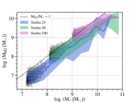
The left panel of Fig. 12 is an alternative way to show the information displayed in the middle panel of Fig. 1, by replacing the plotting method with hexbin contours and showing molecular gas mass on the y axis instead of molecular to stellar mass fraction. The median molecular gas mass is shown on top of the hexbin contours for each simulation box separately. In Fig. 1, the different simulation box sizes seem inconsistent with each other, but when looking at Fig. 12 the in-continuities largely go away, and we instead see a slightly increasing molecular gas mass fraction with stellar mass. Unfortunately we do not properly cover the stellar mass range $>10^{10}\,$$M_{\odot}$ to compare with observations showing a slight downward trend of $M_{\rm mol}/M_{*}$ fractions with stellar mass in this high mass range (Saintonge et al. 2011). The right panel of Fig. 12 shows how the [CII] luminosity per molecular gas mass corresponds to a common [CII] molecular gas mass conversion factor across the different simba volumes. The use of $L_{\rm[CII]}$ as a gas mass tracer with this data is currently being investigated in a separate paper.

Figure 12.— Left: Molecular mass against stellar mass for the entire simba galaxy sample (grey hexbin contours) and median molecular mass for each simulation box separately. Shaded areas indicate the 0.05 to 0.95 quantiles around the median values. A black dashed line indicates a 1-to-1 relation, showing how the molecular to stellar mass fraction generally increases with stellar mass for the simba simulations. Right: [CII] luminosity against molecular mass for all simba volumes with the same plotting technique. Despite the increase in molecular to stellar mass fraction, all volumes agree with a common [CII] molecular gas mass factor.

Appendix B Elemental Abundances

In cloudy, one can supply the total metallicity, where the abundance of each elements is then scaled assuming the Solar composition. We account for abundance patterns of galaxies that differ from Solar using the abundance ratio for each elements tracked in simba (i.e., He, C, N, O, Ne, Mg, Si, S, Ca, and Fe). Since the mass fraction of each element varies as a function of metallicity, we determine its running means for each element using all the gas fluid elements of the simba galaxies studied here. This yields a function that maps a given metallicity to an abundance pattern (see Figure 13), such that for a given metallicity of the clouds, the relative elemental abundances in the cloudy input are scaled to reflect the (average) abundance ratio from simba. For more details on this procedure, we refer interested readers to Olsen et al. (2017).

Figure 13.— Gray hexbins represent the mass fractions of each elements tracked in simba as function of metallicity for all gas fluid elements. A running mean is determined for each element as a function of metallicity (blue line). The green lines show the Solar abundance as a function of metallicity, after scaling by the respective factors determined in order to match the abundance ratio from simba (blue). These factors yield a mapping function that enables the cloudy input to reflect the abundance ratio of the simba galaxies that differ from Solar.

Appendix C $L_{\rm[CII]}$– SFR Relation and DTM

In Figure 14, we show the effects of adopting a different DTM ratio on the $L_{\rm[CII]}$– SFR relation, in particular, using a Solar DTM following Olsen et al. (2017) ($\xi_{\rm DTM}$ = 0.46) instead of the mean DTM ratio found in the simba sample ($\xi_{\rm DTM}$ = 0.25). Using the former ratio, the [CII] luminosity is approximately $\lesssim$ 0.5 dex lower (cf. Olsen et al. 2017 who finds that the $L_{\rm[CII]}$ is only $\sim$ 0.15 dex lower at the same SFR for their Mufasa SFMS sample).

Figure 14.— $L_{\rm[CII]}$– SFR of simba galaxies when adopting the mean DTM of the simba sample (red line) and when adopting a Solar DTM (cyan line). Adopting the lower DTM results in predicted [CII] luminosities at fixed SFR that are about 0.5 lower than those with a Solar DTM.

References

- Aird et al. (2019) Aird, J., Coil, A. L., & Georgakakis, A. 2019, MNRAS, 484, 4360, doi: 10.1093/mnras/stz125
- Allen et al. (2008) Allen, M. G., Groves, B. A., Dopita, M. A., Sutherland, R. S., & Kewley, L. J. 2008, ApJS, 178, 20, doi: 10.1086/589652
- Allende Prieto et al. (2002) Allende Prieto, C., Lambert, D. L., & Asplund, M. 2002, ApJ, 573, L137, doi: 10.1086/342095
- Anglés-Alcázar et al. (2017a) Anglés-Alcázar, D., Davé, R., Faucher-Giguère, C.-A., Özel, F., & Hopkins, P. F. 2017a, MNRAS, 464, 2840, doi: 10.1093/mnras/stw2565
- Anglés-Alcázar et al. (2017b) Anglés-Alcázar, D., Faucher-Giguère, C.-A., Kereš, D., et al. 2017b, MNRAS, 470, 4698, doi: 10.1093/mnras/stx1517
- Appleby et al. (2020) Appleby, S., Davé, R., Kraljic, K., Anglés-Alcázar, D., & Narayanan, D. 2020, MNRAS, 494, 6053, doi: 10.1093/mnras/staa1169
- Aravena et al. (2016) Aravena, M., Spilker, J. S., Bethermin, M., et al. 2016, MNRAS, 457, 4406, doi: 10.1093/mnras/stw275
- Asplund et al. (2009) Asplund, M., Grevesse, N., Sauval, A. J., & Scott, P. 2009, ARA&A, 47, 481, doi: 10.1146/annurev.astro.46.060407.145222
- Astropy Collaboration et al. (2013) Astropy Collaboration, Robitaille, T. P., Tollerud, E. J., et al. 2013, A&A, 558, A33, doi: 10.1051/0004-6361/201322068
- Bayet et al. (2009) Bayet, E., Viti, S., Williams, D. A., Rawlings, J. M. C., & Bell, T. 2009, ApJ, 696, 1466, doi: 10.1088/0004-637X/696/2/1466
- Behroozi et al. (2013) Behroozi, P. S., Wechsler, R. H., & Conroy, C. 2013, ApJ, 762, L31, doi: 10.1088/2041-8205/762/2/L31
- Blitz et al. (2007) Blitz, L., Fukui, Y., Kawamura, A., et al. 2007, Protostars and Planets V, 81
- Bouwens et al. (2015) Bouwens, R. J., Illingworth, G. D., Oesch, P. A., et al. 2015, ApJ, 803, 34, doi: 10.1088/0004-637X/803/1/34
- Bradač et al. (2017) Bradač, M., Garcia-Appadoo, D., Huang, K.-H., et al. 2017, ApJ, 836, L2, doi: 10.3847/2041-8213/836/1/L2
- Bruzual & Charlot (2003) Bruzual, G., & Charlot, S. 2003, MNRAS, 344, 1000, doi: 10.1046/j.1365-8711.2003.06897.x
- Calzetti (2001) Calzetti, D. 2001, PASP, 113, 1449, doi: 10.1086/324269
- Camps & Baes (2015) Camps, P., & Baes, M. 2015, Astronomy and Computing, 9, 20, doi: 10.1016/j.ascom.2014.10.004
- Capak et al. (2015) Capak, P. L., Carilli, C., Jones, G., et al. 2015, Nature, 522, 455, doi: 10.1038/nature14500
- Carniani et al. (2018a) Carniani, S., Maiolino, R., Amorin, R., et al. 2018a, MNRAS, 478, 1170, doi: 10.1093/mnras/sty1088
- Carniani et al. (2018b) —. 2018b, MNRAS, 478, 1170, doi: 10.1093/mnras/sty1088
- Chung et al. (2019) Chung, D. T., Viero, M. P., Church, S. E., et al. 2019, ApJ, 872, 186, doi: 10.3847/1538-4357/ab0027
- Cooray et al. (2019) Cooray, A., Aguirre, J., Ali-Haimoud, Y., et al. 2019, BAAS, 51, 48. https://arxiv.org/abs/1903.03629
- Cowie & Songaila (1986) Cowie, L. L., & Songaila, A. 1986, ARA&A, 24, 499, doi: 10.1146/annurev.aa.24.090186.002435
- da Cunha et al. (2013) da Cunha, E., Groves, B., Walter, F., et al. 2013, ApJ, 766, 13, doi: 10.1088/0004-637X/766/1/13
- Davé et al. (2019) Davé, R., Anglés-Alcázar, D., Narayanan, D., et al. 2019, MNRAS, 486, 2827, doi: 10.1093/mnras/stz937
- Davé et al. (2020) Davé, R., Crain, R. A., Stevens, A. R. H., et al. 2020, arXiv e-prints, arXiv:2002.07226. https://arxiv.org/abs/2002.07226
- Davé et al. (2016) Davé, R., Thompson, R., & Hopkins, P. F. 2016, MNRAS, 462, 3265, doi: 10.1093/mnras/stw1862
- De Looze et al. (2014) De Looze, I., Cormier, D., Lebouteiller, V., et al. 2014, A&A, 568, A62, doi: 10.1051/0004-6361/201322489
- De Vis et al. (2019) De Vis, P., Jones, A., Viaene, S., et al. 2019, A&A, 623, A5, doi: 10.1051/0004-6361/201834444
- Decarli et al. (2017) Decarli, R., Walter, F., Venemans, B. P., et al. 2017, Nature, 545, 457, doi: 10.1038/nature22358
- Díaz-Santos et al. (2014) Díaz-Santos, T., Armus, L., Charmandaris, V., et al. 2014, ApJ, 788, L17, doi: 10.1088/2041-8205/788/1/L17
- Ferland et al. (2017) Ferland, G. J., Chatzikos, M., Guzmán, F., et al. 2017, Rev. Mexicana Astron. Astrofis., 53, 385. https://arxiv.org/abs/1705.10877
- Finkelstein (2016) Finkelstein, S. L. 2016, PASA, 33, e037, doi: 10.1017/pasa.2016.26
- Gong et al. (2012) Gong, Y., Cooray, A., Silva, M., et al. 2012, ApJ, 745, 49, doi: 10.1088/0004-637X/745/1/49
- González-López et al. (2014) González-López, J., Riechers, D. A., Decarli, R., et al. 2014, ApJ, 784, 99, doi: 10.1088/0004-637X/784/2/99
- Hashimoto et al. (2019) Hashimoto, T., Inoue, A. K., Mawatari, K., et al. 2019, PASJ, 71, 71, doi: 10.1093/pasj/psz049
- Hayward et al. (2013) Hayward, C. C., Behroozi, P. S., Somerville, R. S., et al. 2013, MNRAS, 434, 2572, doi: 10.1093/mnras/stt1202
- Hemmati et al. (2017) Hemmati, S., Yan, L., Diaz-Santos, T., et al. 2017, ApJ, 834, 36, doi: 10.3847/1538-4357/834/1/36
- Herrera-Camus et al. (2015) Herrera-Camus, R., Bolatto, A. D., Wolfire, M. G., et al. 2015, ApJ, 800, 1, doi: 10.1088/0004-637X/800/1/1
- Hickox & Alexander (2018) Hickox, R. C., & Alexander, D. M. 2018, ARA&A, 56, 625, doi: 10.1146/annurev-astro-081817-051803
- Hodge & da Cunha (2020) Hodge, J. A., & da Cunha, E. 2020, arXiv e-prints, arXiv:2004.00934. https://arxiv.org/abs/2004.00934
- Hunter (2007) Hunter, J. D. 2007, Computing in Science Engineering, 9, 90, doi: 10.1109/MCSE.2007.55
- Inami et al. (2017) Inami, H., Bacon, R., Brinchmann, J., et al. 2017, A&A, 608, A2, doi: 10.1051/0004-6361/201731195
- Inoue et al. (2016) Inoue, S., Dekel, A., Mandelker, N., et al. 2016, MNRAS, 456, 2052, doi: 10.1093/mnras/stv2793
- Inoue et al. (2020) Inoue, S., Yoshida, N., & Yajima, H. 2020, arXiv e-prints, arXiv:2008.12484. https://arxiv.org/abs/2008.12484
- Iyer et al. (2018) Iyer, K., Gawiser, E., Davé, R., et al. 2018, ApJ, 866, 120, doi: 10.3847/1538-4357/aae0fa
- Jiang et al. (2016) Jiang, L., Finlator, K., Cohen, S. H., et al. 2016, ApJ, 816, 16, doi: 10.3847/0004-637X/816/1/16
- Jones et al. (2001–) Jones, E., Oliphant, T., Peterson, P., et al. 2001–, SciPy: Open source scientific tools for Python. http://www.scipy.org/
- Jones et al. (2017) Jones, G. C., Carilli, C. L., Shao, Y., et al. 2017, ApJ, 850, 180, doi: 10.3847/1538-4357/aa8df2
- Kanekar et al. (2013) Kanekar, N., Wagg, J., Chary, R. R., & Carilli, C. L. 2013, ApJ, 771, L20, doi: 10.1088/2041-8205/771/2/L20
- Katz et al. (2017) Katz, H., Kimm, T., Sijacki, D., & Haehnelt, M. G. 2017, MNRAS, 468, 4831, doi: 10.1093/mnras/stx608
- Katz et al. (2019) Katz, H., Galligan, T. P., Kimm, T., et al. 2019, MNRAS, 487, 5902, doi: 10.1093/mnras/stz1672
- Kaufman et al. (1999) Kaufman, M. J., Wolfire, M. G., Hollenbach, D. J., & Luhman, M. L. 1999, ApJ, 527, 795, doi: 10.1086/308102
- Kawamata et al. (2018) Kawamata, R., Ishigaki, M., Shimasaku, K., et al. 2018, ApJ, 855, 4, doi: 10.3847/1538-4357/aaa6cf
- Keating et al. (2015) Keating, G. K., Bower, G. C., Marrone, D. P., et al. 2015, ApJ, 814, 140, doi: 10.1088/0004-637X/814/2/140
- Kennicutt & Evans (2012) Kennicutt, R. C., & Evans, N. J. 2012, ARA&A, 50, 531, doi: 10.1146/annurev-astro-081811-125610
- Knudsen et al. (2016) Knudsen, K. K., Richard, J., Kneib, J.-P., et al. 2016, MNRAS, 462, L6, doi: 10.1093/mnrasl/slw114
- Knudsen et al. (2017) Knudsen, K. K., Watson, D., Frayer, D., et al. 2017, MNRAS, 466, 138, doi: 10.1093/mnras/stw3066
- Kovetz et al. (2017) Kovetz, E. D., Viero, M. P., Lidz, A., et al. 2017, arXiv e-prints, arXiv:1709.09066. https://arxiv.org/abs/1709.09066
- Kroupa (2002) Kroupa, P. 2002, Science, 295, 82, doi: 10.1126/science.1067524
- Krumholz (2014) Krumholz, M. R. 2014, MNRAS, 437, 1662, doi: 10.1093/mnras/stt2000
- Lagache et al. (2018) Lagache, G., Cousin, M., & Chatzikos, M. 2018, A&A, 609, A130, doi: 10.1051/0004-6361/201732019
- Leitherer et al. (2014) Leitherer, C., Ekström, S., Meynet, G., et al. 2014, ApJS, 212, 14, doi: 10.1088/0067-0049/212/1/14
- Li et al. (2019) Li, Q., Narayanan, D., & Davé, R. 2019, MNRAS, 490, 1425, doi: 10.1093/mnras/stz2684
- Luhman et al. (2003) Luhman, M. L., Satyapal, S., Fischer, J., et al. 2003, ApJ, 594, 758, doi: 10.1086/376965
- Lupi & Bovino (2020) Lupi, A., & Bovino, S. 2020, MNRAS, 492, 2818, doi: 10.1093/mnras/staa048
- Madau & Dickinson (2014) Madau, P., & Dickinson, M. 2014, ARA&A, 52, 415, doi: 10.1146/annurev-astro-081811-125615
- Maiolino et al. (2008) Maiolino, R., Nagao, T., Grazian, A., et al. 2008, A&A, 488, 463, doi: 10.1051/0004-6361:200809678
- Maiolino et al. (2015) Maiolino, R., Carniani, S., Fontana, A., et al. 2015, MNRAS, 452, 54, doi: 10.1093/mnras/stv1194
- Malhotra et al. (2001) Malhotra, S., Kaufman, M. J., Hollenbach, D., et al. 2001, ApJ, 561, 766, doi: 10.1086/323046
- Mannucci et al. (2010) Mannucci, F., Cresci, G., Maiolino, R., Marconi, A., & Gnerucci, A. 2010, MNRAS, 408, 2115, doi: 10.1111/j.1365-2966.2010.17291.x
- Marrone et al. (2018) Marrone, D. P., Spilker, J. S., Hayward, C. C., et al. 2018, Nature, 553, 51, doi: 10.1038/nature24629
- Matthee et al. (2017) Matthee, J., Sobral, D., Boone, F., et al. 2017, ApJ, 851, 145, doi: 10.3847/1538-4357/aa9931
- McKee & Ostriker (2007) McKee, C. F., & Ostriker, E. C. 2007, ARA&A, 45, 565, doi: 10.1146/annurev.astro.45.051806.110602
- Miller et al. (2016) Miller, T. B., Chapman, S. C., Hayward, C. C., et al. 2016, arXiv e-prints, arXiv:1611.08552. https://arxiv.org/abs/1611.08552
- Narayanan & Krumholz (2017) Narayanan, D., & Krumholz, M. R. 2017, MNRAS, 467, 50, doi: 10.1093/mnras/stw3218
- Narayanan et al. (2015) Narayanan, D., Turk, M., Feldmann, R., et al. 2015, Nature, 525, 496, doi: 10.1038/nature15383
- Nelson et al. (2018) Nelson, D., Pillepich, A., Springel, V., et al. 2018, MNRAS, 475, 624, doi: 10.1093/mnras/stx3040
- Oesch et al. (2016) Oesch, P. A., Brammer, G., van Dokkum, P. G., et al. 2016, ApJ, 819, 129, doi: 10.3847/0004-637X/819/2/129
- Olsen et al. (2017) Olsen, K., Greve, T. R., Narayanan, D., et al. 2017, ApJ, 846, 105, doi: 10.3847/1538-4357/aa86b4
- Olsen et al. (2015) Olsen, K. P., Greve, T. R., Narayanan, D., et al. 2015, ApJ, 814, 76, doi: 10.1088/0004-637X/814/1/76
- Olsen et al. (2018) Olsen, K. P., Pallottini, A., Wofford, A., et al. 2018, ArXiv e-prints. https://arxiv.org/abs/1808.08251
- Oppenheimer & Davé (2006) Oppenheimer, B. D., & Davé, R. 2006, MNRAS, 373, 1265, doi: 10.1111/j.1365-2966.2006.10989.x
- Ota et al. (2014) Ota, K., Walter, F., Ohta, K., et al. 2014, ApJ, 792, 34, doi: 10.1088/0004-637X/792/1/34
- Ouchi et al. (2013) Ouchi, M., Ellis, R., Ono, Y., et al. 2013, ApJ, 778, 102, doi: 10.1088/0004-637X/778/2/102
- Pallottini et al. (2017a) Pallottini, A., Ferrara, A., Bovino, S., et al. 2017a, MNRAS, 471, 4128, doi: 10.1093/mnras/stx1792
- Pallottini et al. (2017b) Pallottini, A., Ferrara, A., Gallerani, S., et al. 2017b, MNRAS, 465, 2540, doi: 10.1093/mnras/stw2847
- Pallottini et al. (2019) Pallottini, A., Ferrara, A., Decataldo, D., et al. 2019, MNRAS, 487, 1689, doi: 10.1093/mnras/stz1383
- Pentericci et al. (2016) Pentericci, L., Carniani, S., Castellano, M., et al. 2016, ApJ, 829, L11, doi: 10.3847/2041-8205/829/1/L11
- Planck Collaboration et al. (2016) Planck Collaboration, Ade, P. A. R., Aghanim, N., et al. 2016, A&A, 594, A13, doi: 10.1051/0004-6361/201525830
- Popping et al. (2019) Popping, G., Narayanan, D., Somerville, R. S., Faisst, A. L., & Krumholz, M. R. 2019, MNRAS, 482, 4906, doi: 10.1093/mnras/sty2969
- Popping et al. (2017) Popping, G., Somerville, R. S., & Galametz, M. 2017, MNRAS, 471, 3152, doi: 10.1093/mnras/stx1545
- Popping et al. (2016) Popping, G., van Kampen, E., Decarli, R., et al. 2016, MNRAS, 461, 93, doi: 10.1093/mnras/stw1323
- Rahmati et al. (2013) Rahmati, A., Pawlik, A. H., Raičević, M., & Schaye, J. 2013, MNRAS, 430, 2427, doi: 10.1093/mnras/stt066
- Rémy-Ruyer et al. (2014) Rémy-Ruyer, A., Madden, S. C., Galliano, F., et al. 2014, A&A, 563, A31, doi: 10.1051/0004-6361/201322803
- Saintonge et al. (2011) Saintonge, A., Kauffmann, G., Kramer, C., et al. 2011, MNRAS, 415, 32, doi: 10.1111/j.1365-2966.2011.18677.x
- Schaerer et al. (2015) Schaerer, D., Boone, F., Zamojski, M., et al. 2015, A&A, 574, A19, doi: 10.1051/0004-6361/201424649
- Silva et al. (2015) Silva, M., Santos, M. G., Cooray, A., & Gong, Y. 2015, ApJ, 806, 209, doi: 10.1088/0004-637X/806/2/209
- Smit et al. (2017) Smit, R., Swinbank, A. M., Massey, R., et al. 2017, MNRAS, 467, 3306, doi: 10.1093/mnras/stx245
- Smit et al. (2018) Smit, R., Bouwens, R. J., Carniani, S., et al. 2018, Nature, 553, 178, doi: 10.1038/nature24631
- Smith et al. (2009) Smith, B. D., Turk, M. J., Sigurdsson, S., O’Shea, B. W., & Norman, M. L. 2009, ApJ, 691, 441, doi: 10.1088/0004-637X/691/1/441
- Somerville & Davé (2015) Somerville, R. S., & Davé, R. 2015, ARA&A, 53, 51, doi: 10.1146/annurev-astro-082812-140951
- Song et al. (2016) Song, M., Finkelstein, S. L., Ashby, M. L. N., et al. 2016, ApJ, 825, 5, doi: 10.3847/0004-637X/825/1/5
- Speagle et al. (2014) Speagle, J. S., Steinhardt, C. L., Capak, P. L., & Silverman, J. D. 2014, ApJS, 214, 15, doi: 10.1088/0067-0049/214/2/15
- Thomas et al. (2019) Thomas, N., Davé, R., Anglés-Alcázar, D., & Jarvis, M. 2019, MNRAS, 487, 5764, doi: 10.1093/mnras/stz1703
- Tress et al. (2020) Tress, R. G., Smith, R. J., Sormani, M. C., et al. 2020, MNRAS, 492, 2973, doi: 10.1093/mnras/stz3600
- Turk et al. (2011) Turk, M. J., Smith, B. D., Oishi, J. S., et al. 2011, ApJS, 192, 9, doi: 10.1088/0067-0049/192/1/9
- Uzgil et al. (2014) Uzgil, B. D., Aguirre, J. E., Bradford, C. M., & Lidz, A. 2014, ApJ, 793, 116, doi: 10.1088/0004-637X/793/2/116
- Vallini et al. (2015) Vallini, L., Gallerani, S., Ferrara, A., Pallottini, A., & Yue, B. 2015, ApJ, 813, 36, doi: 10.1088/0004-637X/813/1/36
- Vallini et al. (2019) Vallini, L., Tielens, A. G. G. M., Pallottini, A., et al. 2019, MNRAS, 490, 4502, doi: 10.1093/mnras/stz2837
- van der Walt et al. (2011) van der Walt, S., Colbert, S. C., & Varoquaux, G. 2011, Computing in Science Engineering, 13, 22, doi: 10.1109/MCSE.2011.37
- Van Rossum & de Boer (1991) Van Rossum, G., & de Boer, J. 1991, CWI Quarterly, 4, 283
- Visbal & Loeb (2010) Visbal, E., & Loeb, A. 2010, J. Cosmology Astropart. Phys, 2010, 016, doi: 10.1088/1475-7516/2010/11/016
- Walter et al. (2016) Walter, F., Decarli, R., Aravena, M., et al. 2016, ApJ, 833, 67, doi: 10.3847/1538-4357/833/1/67
- Wilkins et al. (2019) Wilkins, S. M., Lovell, C. C., & Stanway, E. R. 2019, MNRAS, 490, 5359, doi: 10.1093/mnras/stz2894
- Willott et al. (2015) Willott, C. J., Carilli, C. L., Wagg, J., & Wang, R. 2015, ApJ, 807, 180, doi: 10.1088/0004-637X/807/2/180
- Wu et al. (2019) Wu, X., Davé, R., Tacchella, S., & Lotz, J. 2019, arXiv e-prints, arXiv:1911.06330. https://arxiv.org/abs/1911.06330
- Yang et al. (2020) Yang, S., Somerville, R. S., Pullen, A. R., et al. 2020, arXiv e-prints, arXiv:2009.11933. https://arxiv.org/abs/2009.11933
- Yue & Ferrara (2019) Yue, B., & Ferrara, A. 2019, MNRAS, 490, 1928, doi: 10.1093/mnras/stz2728