On SICA models for HIV transmission

Abstract

We revisit the SICA (Susceptible–Infectious–Chronic–AIDS) mathematical model for transmission dynamics of the human immunodeficiency virus (HIV) with varying population size in a homogeneously mixing population. We consider SICA models given by systems of ordinary differential equations and some generalizations given by systems with fractional and stochastic differential operators. Local and global stability results are proved for deterministic, fractional, and stochastic-type SICA models. Two case studies, in Cape Verde and Morocco, are investigated.

Keywords: HIV/AIDS, SICA compartmental models, Deterministic models, Fractional models, Stochastic models, Stability analysis, Lyapunov functions, Cape Verde and Morocco case studies.

1 Introduction

In this work, we make an overview on SICA compartmental models for HIV/AIDS transmission dynamics with varying population size in a homogeneously mixing population, given by a system of four equations. The SICA model divides the total human population into four mutually-exclusive compartments: susceptible individuals ($S$); HIV-infected individuals with no clinical symptoms of AIDS (the virus is living or developing in the individuals but without producing symptoms or only mild ones) but able to transmit HIV to other individuals ($I$); HIV-infected individuals under antiretroviral therapy (ART), the so called chronic stage with a viral load remaining low ($C$); and HIV-infected individuals with AIDS clinical symptoms ($A$). The total population at time $t$, denoted by $N(t)$, is given by

$$N(t)=S(t)+I(t)+C(t)+A(t).$$

The deterministic SICA model was firstly proposed as a sub-model of a TB–HIV/AIDS co-infection model and published in 2015, see [55]. After, it was generalized to fractional [58] and stochastic systems of differential equations [20] and calibrated to the HIV/AIDS epidemic situation in Cape Verde [56, 57] and Morocco [40]. One of the main goals of SICA models is to show that a simple mathematical model can help to clarify some of the essential relations between epidemiological factors and the overall pattern of the AIDS epidemic [46, 56].

The assumptions of the SICA models are now described. The susceptible population is increased by the recruitment of individuals into the population, assumed susceptible, at a rate $\Lambda$. All individuals suffer from natural death, at a constant rate $\mu$. Susceptible individuals $S$ acquire HIV infection, following effective contact with people infected with HIV, at a rate $\lambda$, given by

$$\lambda(t)=\frac{\beta}{N(t)}\left(I(t)+\eta_{C}\,C(t)+\eta_{A}A(t)\right),$$ (1)

where $\beta$ is the effective contact rate for HIV transmission. The modification parameter $\eta_{A}\geq 1$ accounts for the relative infectiousness of individuals with AIDS symptoms, in comparison to those infected with HIV with no AIDS symptoms. Individuals with AIDS symptoms are more infectious than HIV-infected individuals (pre-AIDS) because they have a higher viral load and there is a positive correlation between viral load and infectiousness [63]. On the other hand, $\eta_{C}\leq 1$ translates the partial restoration of immune function of individuals with HIV infection that use correctly ART [16].

HIV-infected individuals, with and without AIDS symptoms, have access to ART treatment. HIV-infected individuals with no AIDS symptoms, $I$, progress to the class of individuals with HIV infection under ART treatment $C$ at a rate $\phi$, and HIV-infected individuals with AIDS symptoms are treated for HIV at rate $\gamma$. An HIV-infected individual with AIDS symptoms, $A$, that starts treatment, moves to the class of HIV-infected individuals, $I$, and will move to the chronic class, $C$, only if the treatment is maintained. HIV-infected individuals with no AIDS symptoms, $I$, that do not take ART treatment, progress to the AIDS class, $A$, at rate $\rho$. Only HIV-infected individuals with AIDS symptoms $A$ suffer from an AIDS induced death, at a rate $d$. These assumptions are translated into the following mathematical model, given by a system of four ordinary differential equations:

$$\begin{cases}\dot{S}(t)=\Lambda-\beta\lambda(t)S(t)-\mu S(t),\\[5.69046pt] \dot{I}(t)=\beta\lambda(t)S(t)-(\rho+\phi+\mu)I(t)+\gamma A(t)+\omega C(t),\\[5.69046pt] \dot{C}(t)=\phi I(t)-(\omega+\mu)C(t),\\[5.69046pt] \dot{A}(t)=\rho\,I(t)-(\gamma+\mu+d)A(t).\end{cases}$$ (2)

The region

$$\Omega=\biggl{\{}\left(S,I,C,A\right)\in\mathbb{R}_{+}^{4}\,:\,N\leq\Lambda/\mu\biggr{\}}$$ (3)

is positively invariant and attracting [55]. Thus, the dynamics of the HIV model evolves in $\Omega$.

Model (2) has a disease-free equilibrium, given by

$$\Sigma_{0}=\left(S^{0},I^{0},C^{0},A^{0}\right)=\left(\frac{\Lambda}{\mu},0,0,0\right).$$ (4)

Following the approach from [60], the basic reproduction number $R_{0}$ for model (2), which represents the expected average number of new HIV infections produced by a single HIV-infected individual when in contact with a completely susceptible population, is given by

$$R_{0}=\frac{\beta\,\left(\xi_{2}\left(\xi_{1}+\rho\,\eta_{A}\right)+\eta_{C}\,\phi\,\xi_{1}\right)}{\mu\,\left(\xi_{2}\left(\rho+\xi_{1}\right)+\phi\,\xi_{1}+\rho\,d\right)+\rho\,\omega\,d}=\frac{\mathcal{N}}{\mathcal{D}},$$ (5)

where along all manuscript $\xi_{1}=\gamma+\mu+d$, $\xi_{2}=\omega+\mu$, and $\xi_{3}=\rho+\phi+\mu$, see [57].

To find conditions for the existence of an equilibrium for which HIV is endemic in the population (i.e., at least one of $I^{*}$, $C^{*}$ or $A^{*}$ is nonzero), denoted by $\Sigma_{+}=\left(S^{*},I^{*},C^{*},A^{*}\right)$, the equations in (2) are solved in terms of the force of infection at the steady-state $\lambda^{*}$, given by

$$\lambda^{*}=\frac{\beta\left(I^{*}+\eta_{C}\,C^{*}+\eta_{A}A^{*}\right)}{N^{*}}.$$ (6)

Setting the right hand side of the equations of the model to zero, and noting that $\lambda=\lambda^{*}$ at equilibrium gives

$$S^{*}=\frac{\Lambda}{\lambda^{*}+\mu}\,,\quad I^{*}=-\frac{\lambda^{*}\Lambda\xi_{1}\xi_{2}}{D}\,,\quad C^{*}=-\frac{\phi\lambda^{*}\Lambda\xi_{1}}{D}\,,\quad A^{*}=-\frac{\rho_{1}\lambda^{*}\Lambda\xi_{2}}{D}$$ (7)

with $D=-\left(\lambda^{*}+\mu\right)\left(\mu\left(\xi_{2}(\rho+\xi_{1})+\xi_{1}\phi+\rho d\right)+\rho\omega d\right)$, we use (7) in the expression for $\lambda^{*}$ in (6) to show that the nonzero (endemic) equilibrium of the model satisfies

$$\lambda^{*}=-\mu(1-R_{0}).$$

The force of infection at the steady-state $\lambda^{*}$ is positive only if $R_{0}>1$. Thus, the existence and uniqueness of the endemic equilibrium follows.

Remark 1.1.

The explicit expression of the endemic equilibrium $\Sigma_{+}$ of model (2) is given by

$$\begin{split}S^{*}&=\frac{\Lambda(\rho d\xi_{2}-\mathcal{D})}{\mu(\rho d\xi_{2}-\mathcal{N})}\,,\quad\quad I^{*}=\frac{\Lambda\xi_{1}\xi_{2}(\mathcal{D}-\mathcal{N})}{\mathcal{D}(\rho d\xi_{2}-\mathcal{N})}\,,\\ C^{*}&=\frac{\Lambda\phi\xi_{1}(\mathcal{D}-\mathcal{N})}{\mathcal{D}(\rho d\xi_{2}-\mathcal{N})}\,,\quad\quad A^{*}=\frac{\Lambda\rho\xi_{2}(\mathcal{D}-\mathcal{N})}{\mathcal{D}(\rho d\xi_{2}-\mathcal{N})}.\end{split}$$ (8)

Adding the equations of model (2), with $d=0$, gives $\dot{N}=\Lambda-\mu N$, so that $N\to\frac{\Lambda}{\mu}$ as $t\to\infty$. Thus, $\frac{\Lambda}{\mu}$ is an upper bound of $N(t)$ provided that $N(0)\leq\frac{\Lambda}{\mu}$. Further, if $N(0)>\frac{\Lambda}{\mu}$, then $N(t)$ decreases to this level. Using $N=\frac{\Lambda}{\mu}$ in the force of infection $\lambda=\frac{\beta}{N}\left(I+\eta_{C}\,C+\eta_{A}A\right)$ gives a limiting (mass action) system (see, e.g., [1]). Then, the force of infection becomes

$$\lambda=\beta_{1}\left(I+\eta_{C}\,C+\eta_{A}A\right)\,,\quad\text{where}\quad\beta_{1}=\frac{\beta\mu}{\Lambda}.$$

Therefore, we have the following model:

$$\begin{cases}\dot{S}(t)=\Lambda-\beta_{1}\left(I(t)+\eta_{C}\,C(t)+\eta_{A}A(t)\right)S(t)-\mu S(t),\\[5.69046pt] \dot{I}(t)=\beta_{1}\left(I(t)+\eta_{C}\,C(t)+\eta_{A}A(t)\right)S(t)-\xi_{3}I(t)+\gamma A(t)+\omega C(t),\\[5.69046pt] \dot{C}(t)=\phi I(t)-\xi_{2}C(t),\\[5.69046pt] \dot{A}(t)=\rho\,I(t)-\xi_{1}A(t),\end{cases}$$ (9)

where $\xi_{1}=\gamma+\mu$. Here, different mathematical models based on (2) and (9) are considered.

The paper is organized as follows. In Section 2, a general fractional SICA model is proposed and the uniform stability of the equilibrium points is given. In Section 3, a stochastic environmental noise is introduced into the SICA model (9). Existence and uniqueness of a positive global solution is proved and conditions for the extinction and persistence in mean of the disease are provided. In Section 4, the deterministic model is analyzed, proving the uniform persistence of the total population and local and global stability of the equilibrium points, through Lyapunov’s direct method and LaSalle’s invariance principle. Lyapunov functions are provided. Then, with Section 5, two case studies are analyzed, being shown that models (2) and (9), after an adequate calibration of the parameters, describe well the HIV/AIDS situation in Cape Verde and Morocco from 1987 to 2014 and 1986 to 2015, respectively. The paper ends with Section 6 of conclusion.

2 Fractional SICA model

Fractional differential equations (FDEs), also known in the literature as extraordinary differential equations, are a generalization of differential equations through the application of fractional calculus, that is, the branch of mathematical analysis that studies different possibilities of defining differentiation operators of noninteger order [3, 22, 58].

FDEs are naturally related to systems with memory, which explains their usefulness in most biological systems [49]. Indeed, FDEs have been considered in many epidemiological models [58].

In this section, we analyze the general fractional SICA model and its uniform stability, proved in [58]. We first recall some important definitions and results that are used in the proofs of the uniform asymptotic stability of the equilibrium points.

2.1 Preliminaries: fractional calculus and uniform asymptotic stability

We begin by recalling the definition of Caputo fractional derivative.

Definition 2.1 (See [8]).

Let $a>0$, $t>a$, and $\alpha,a,t\in\mathbb{R}$. The Caputo fractional derivative of order $\alpha$ of a function $f\in C^{n}$ is given by

$${}_{a}^{C}D_{t}^{\alpha}f(t)=\dfrac{1}{\Gamma(n-\alpha)}\int_{a}^{t}\dfrac{f^{(n)}(\xi)}{(t-\xi)^{\alpha+1-n}}d\xi,\qquad n-1<\alpha<n\in\mathbb{N}.$$

Let us consider the following general fractional differential equation involving the Caputo derivative:

$$_{a}^{C}D_{t}^{\alpha}x(t)=f(t,x(t)),\qquad\alpha\in(0,1),$$ (10)

subject to a given initial condition $x_{0}=x(t_{0})$.

Definition 2.2 (See, e.g., [37]).

The constant $x^{*}$ is an equilibrium point of the Caputo fractional dynamic system (10) if, and only if, $f(t,x^{*})=0$.

We recall an extension of the celebrated Lyapunov direct method for Caputo type fractional order nonlinear systems [18].

Theorem 2.3 (Uniform Asymptotic Stability [18]).

Let $x^{*}$ be an equilibrium point for the nonautonomous fractional order system (10) and $\Omega\subset\mathbb{R}^{n}$ be a domain containing $x^{*}$. Let $L:[0,\infty)\times\Omega\rightarrow\mathbb{R}$ be a continuously differentiable function such that

$$W_{1}(x)\leq L(t,x(t))\leq W_{2}(x)$$

and

$${}_{a}^{C}D_{t}^{\alpha}L(t,x(t))\leq-W_{3}(x)$$

for all $\alpha\in(0,1)$ and all $x\in\Omega$, where $W_{1}(\cdot)$, $W_{2}(\cdot)$ and $W_{3}(\cdot)$ are continuous positive definite functions on $\Omega$. Then the equilibrium point $x^{*}$ of system (10) is uniformly asymptotically stable.

A useful lemma is proved in [61], where a Volterra-type Lyapunov function is obtained for fractional-order epidemic systems.

Lemma 2.4 (See [61]).

Let $x(\cdot)$ be a continuous and differentiable function with $x(t)\in\mathbb{R_{+}}$. Then, for any time instant $t\geq t_{0}$, one has

$${}_{t_{0}}^{C}D_{t}^{\alpha}\left[x(t)-x^{*}-x^{*}\ln\dfrac{x(t)}{x^{*}}\right]\leq\left(1-\dfrac{x^{*}}{x(t)}\right)\,{{}_{t_{0}}^{C}D}_{t}^{\alpha}x(t),\qquad x^{*}\in\mathbb{R}^{+},\qquad\forall\alpha\in(0,1).$$

2.2 Fractional SICA model: local and uniform stability analysis

Let us consider the Caputo fractional order SICA epidemiological model for HIV/AIDS transmission with constant recruitment rate, mass action incidence, and variable population size, firstly proposed in [58]:

$$\begin{cases}{}_{t_{0}}^{C}D_{t}^{\alpha}S(t)=\Lambda-\beta\left(I(t)+\eta_{C}\,C(t)+\eta_{A}A(t)\right)S(t)-\mu S(t),\\[5.69046pt] {}_{t_{0}}^{C}D_{t}^{\alpha}I(t)=\beta\left(I(t)+\eta_{C}\,C(t)+\eta_{A}A(t)\right)S(t)-\xi_{3}I(t)+\omega C(t)+\gamma A(t),\\[5.69046pt] {}_{t_{0}}^{C}D_{t}^{\alpha}C(t)=\phi I(t)-\xi_{2}C(t),\\[5.69046pt] {}_{t_{0}}^{C}D_{t}^{\alpha}A(t)=\rho\,I(t)-\xi_{1}A(t).\end{cases}$$ (11)

The local asymptotic stability of the disease free equilibrium $\Sigma_{0}$ (4), comes straightforward from [45] and [2]. Stronger stability results are stated next.

Theorem 2.5 (See [58]).

Let $\alpha\in(0,1)$. The disease free equilibrium $\Sigma_{0}$ (4), of the fractional order system (11), is uniformly asymptotically stable in $\Omega$ (3), whenever (5) satisfies $R_{0}<1$.

The uniform asymptotic stability of the disease free equilibrium $\Sigma_{0}$ (4) and endemic equilibrium $\Sigma_{+}$ (8) of the fractional order system (11) are based on Theorem 2.3 and Lemma 2.4.

Theorem 2.6 (See [58]).

Let $\alpha\in(0,1)$ and (5) be such that $R_{0}>1$. Then the unique endemic equilibrium $\Sigma_{+}$ (8) of the fractional order system (11) is uniformly asymptotically stable in the interior of $\Omega$ (3).

For the numerical implementation of the fractional derivatives, the implementation of the Adams–Bashforth–Moulton scheme is carried out in [58], which is based in the Matlab code fde12 by Garrappa [21]. This code implements a predictor-corrector PECE method of Adams–Bashforth–Moulton type, as described in [19].

3 Stochastic SICA model

Here, we begin with the deterministic SICA epidemic model for HIV transmission (9). Then, following [23, 24, 25, 43, 59, 67], a stochastic environmental noise is introduced making the model biologically more realistic. Precisely, we consider the model

$$\begin{cases}dS(t)=\left[\Lambda-\beta\left(I(t)+\eta_{C}\,C(t)+\eta_{A}A(t)\right)S(t)-\mu S(t)\right]dt,\\[5.69046pt] dI(t)=\left[\beta\left(I(t)+\eta_{C}\,C(t)+\eta_{A}A(t)\right)S(t)-\xi_{3}I(t)+\gamma A(t)+\omega C(t)\right]dt,\\[5.69046pt] dC(t)=\left[\phi I(t)-\xi_{2}C(t)\right]dt,\\[5.69046pt] dA(t)=\left[\rho\,I(t)-\xi_{1}A(t)\right]dt.\end{cases}$$

Next, the fluctuations in the environment are assumed to manifest themselves in the transmission coefficient rate $\beta$, so that $\beta\rightarrow\beta+\sigma\dot{B}(t)$, where $B(t)$ is a standard Brownian motion with intensity $\sigma^{2}>0$. The stochastic model takes then the following form (see [20]):

$$\begin{cases}dS(t)=\left[\Lambda-\beta\left(I(t)+\eta_{C}\,C(t)+\eta_{A}A(t)\right)S(t)-\mu S(t)\right]dt\\ \qquad\qquad-\sigma\left(I(t)+\eta_{C}\,C(t)+\eta_{A}A(t)\right)S(t)dB(t),\\[5.69046pt] dI(t)=\left[\beta\left(I(t)+\eta_{C}\,C(t)+\eta_{A}A(t)\right)S(t)-\xi_{3}I(t)+\gamma A(t)+\omega C(t)\right]dt\\ \qquad\qquad+\sigma\left(I(t)+\eta_{C}\,C(t)+\eta_{A}A(t)\right)S(t)dB(t),\\[5.69046pt] dC(t)=\left[\phi I(t)-\xi_{2}C(t)\right]dt,\\[5.69046pt] dA(t)=\left[\rho\,I(t)-\xi_{1}A(t)\right]dt.\end{cases}$$ (12)

Let $(\Omega,\mathcal{F},\{\mathcal{F}\}_{t\geq 0},\mathcal{P})$ be a complete probability space with filtration $\{\mathcal{F}\}_{t\geq 0}$, which is right continuous and such that $\mathcal{F}$ contains all $\mathcal{P}$-null sets. The scalar Brownian motion $B(t)$ of (12) is defined on the given probability space. Moreover, denote $\mathbb{R}_{+}^{4}=\left\{(x_{1},x_{2},x_{3},x_{4})|x_{i}>0,i=\overline{1,4}\right\}$.

The existence and uniqueness of a positive global solution of model (12) is easily proved using similar arguments as the ones used in [35].

Theorem 3.1 (See [20]).

For any $t\geq 0$ and any initial value $\left(S(0),I(0),C(0),A(0)\right)\in\mathbb{R}_{+}^{4}$, there is a unique solution $\left(S(t),I(t),C(t),A(t)\right)$ to the SDE (12) and the solution remains in $\mathbb{R}_{+}^{4}$ with probability one. Moreover,

$$N(t)\to\frac{\Lambda}{\mu}\mbox{ as }t\to\infty,$$

where $N(t)=S(t)+I(t)+C(t)+A(t)$.

The next theorem provides a condition for the extinction of the disease.

Theorem 3.2 (See [20]).

Let $Y(t)=\left(S(t),I(t),C(t),A(t)\right)$ be the solution of system (12) with positive initial value. Assume that $\sigma^{2}>\frac{\beta}{2\xi_{3}}$. Then,

$$I(t),C(t),A(t)\rightarrow 0\text{ a.s. and }S(t)\to\displaystyle\frac{\Lambda}{\mu}\text{ a.s.},$$

as $t\to+\infty$.

Let us now recall the notion of persistence in mean.

Definition 3.3.

System (12) is said to be persistent in mean if $\displaystyle\lim_{t\rightarrow\infty}\frac{1}{t}\int_{0}^{t}I(s)ds>0$ a.s.

In what follows, we use the notation

$$[I(t)]:=\displaystyle\frac{1}{t}\int_{0}^{t}I(s)ds.$$

Theorem 3.4.

Let

$$K_{1}=\frac{\beta}{\mu}\left(\frac{\gamma\rho}{\xi_{1}}-\xi_{3}+\frac{\omega\phi}{\xi_{2}}\right)+\frac{\mu(\xi_{1}\xi_{2}-\mu)}{\Lambda(1+\eta_{C}+\eta_{A})}.$$ (13)

For any initial value $(S(0),I(0),C(0),A(0))\in\mathbb{R}_{+}^{4}$ such that

$$S(t)+I(t)+C(t)+A(t)=N(t)\to\frac{\Lambda}{\mu}\text{ as }t\to\infty,$$

if $K_{1}\neq 0$, $\frac{1}{K_{1}}\left(\frac{\Lambda\beta}{\mu}-\xi_{1}\xi_{2}-\frac{\sigma^{2}\Lambda^{2}}{2\mu^{2}}\right)>0$ and $\xi_{1},\xi_{2}>1$, then the solution $(S(t),I(t),C(t),A(t))$ satisfies

$$\liminf_{t\rightarrow\infty}[I(t)]\geq\frac{1}{K_{1}}\left(\frac{\Lambda\beta}{\mu}-\xi_{1}\xi_{2}-\frac{\sigma^{2}\Lambda^{2}}{2\mu^{2}}\right).$$

Proofs of Theorems 3.2 and 3.4 follow the large number theorem for martingales [24] and L’Hôpital’s rule, after applying Itô’s formula in an appropriate way. For numerical simulations that illustrate Theorems 3.2 and 3.4, see [20].

4 Deterministic SICA model

Let us first consider model (2), that we recall here:

$$\begin{cases}\dot{S}(t)=\Lambda-\beta\lambda(t)\frac{\beta}{N(t)}\left(I(t)+\eta_{C}\,C(t)+\eta_{A}A(t)\right)S(t)-\mu S(t),\\[5.69046pt] \dot{I}(t)=\beta\lambda(t)\frac{\beta}{N(t)}\left(I(t)+\eta_{C}\,C(t)+\eta_{A}A(t)\right)S(t)-\xi_{3}I(t)+\gamma A(t)+\omega C(t),\\[5.69046pt] \dot{C}(t)=\phi I(t)-\xi_{2}C(t),\\[5.69046pt] \dot{A}(t)=\rho\,I(t)-\xi_{1}A(t).\end{cases}$$

Theorem 4.1 (See [55]).

The population $N(t)$ is uniformly persistent, that is,

$$\liminf_{t\to\infty}N(t)\geq\varepsilon$$

with $\varepsilon>0$ not depending on the initial data.

The local and global stability analysis of the disease free equilibrium $\Sigma_{0}$ given by (4) and endemic equilibrium point $\Sigma_{+}$ given by (8) is derived in [55]. The local asymptotic stability of the disease-free equilibrium, $\Sigma_{0}$, follows from Theorem 2 of [60], and holds whenever $R_{0}<1$.

Lemma 4.2 (See [55]).

The disease free equilibrium $\Sigma_{0}$ is locally asymptotically stable if $R_{0}<1$, and unstable if $R_{0}>1$.

The global asymptotic stability of the disease free equilibrium $\Sigma_{0}$ is proved in [55], following [10].

Theorem 4.3 (See [55]).

The disease free equilibrium $\Sigma_{0}$ is globally asymptotically stable for $R_{0}<1$.

For the endemic equilibrium point, existence and local asymptotic stability holds whenever $R_{0}>1$.

Lemma 4.4 (See [55]).

The model (2) has a unique endemic equilibrium whenever $R_{0}>1$.

The local asymptotic stability of the endemic equilibrium $\Sigma_{+}$, can be proved using the center manifold theory [9], as described in [11, Theorem 4.1].

Theorem 4.5 (See [55]).

The endemic equilibrium $\Sigma_{+}$ is locally asymptotically stable for $R_{0}\simeq 1$.

Now, assume that the AIDS-induced death rate can be neglected, i.e., $d=0$, and consider the deterministic SICA model given by (9). The model (9) has a unique endemic equilibrium given by $\tilde{\Sigma}_{+}=\Sigma_{+}|_{d=0}$, whenever $\tilde{R}_{0}=R_{0}|_{d=0}>1$. Defining

$$\Omega_{0}=\left\{\left(S,I,C,A\right)\in\Omega\,:\,I=C=A=0\right\},$$

and considering the Lyapunov function

$$V=\left(S-S^{*}\ln(S)\right)+\left(I-I^{*}\ln(I)\right)+\frac{\omega}{\xi_{2}}\left(C-C^{*}\ln(C)\right)+\frac{\gamma}{\xi_{1}}\left(A-A^{*}\ln(A)\right)\,,$$ (14)

it follows from LaSalle’s invariance principle [36] that the endemic equilibrium $\Sigma_{+}$ is globally asymptotically stable.

Theorem 4.6 (See [57]).

The endemic equilibrium $\tilde{\Sigma}_{+}$ of model (9) is globally asymptotically stable in $\Omega\backslash\Omega_{0}$ whenever $\tilde{R}_{0}>1$.

4.1 General incidence function for $\eta_{C}=\eta_{A}=0$

In this subsection, we consider a SICA deterministic model with a general incidence function $f$, and assume that $\eta_{A}=\eta_{C}=0$. The assumption $\eta_{A}=\eta_{C}=0$ is justified by the following arguments:

• although individuals in the chronic stage, with a low viral load and under ART treatment, can still transmit HIV infection, as ART greatly reduces the risk of transmission and individuals that take ART treatment correctly are aware of their health status, one can assume that individuals in the class $C$ do not have risky behaviours for HIV transmission and do not transmit HIV virus, i.e., $\eta_{C}=0$;

• individuals with AIDS clinical symptoms, $A$, are responsible and do not have any behaviour that can transmit HIV infection or, in other cases, are too sick to have a risky behavior, i.e., $\eta_{A}=0$.

Mathematically, the assumption $\eta_{A}=\eta_{C}=0$ translates to the fact that the incidence function $f$ depends only on $S$ and $I$. Accordingly, we consider the SICA deterministic model with a general incidence function $f$ given by (see [40])

$$\begin{cases}\dot{S}(t)=\Lambda-\mu S(t)-f\left(S(t),I(t)\right)I(t),\\[5.69046pt] \dot{I}(t)=f\left(S(t),I(t)\right)I(t)-\xi_{3}I(t)+\gamma A(t)+\omega C(t),\\[5.69046pt] \dot{C}(t)=\phi I(t)-\xi_{2}C(t),\\[5.69046pt] \dot{A}(t)=\rho\,I(t)-\xi_{1}A(t),\end{cases}$$ (15)

with initial conditions

$$S(0)=S_{0}\geq 0,\ I(0)=I_{0}\geq 0,\ C(0)=C_{0}\geq 0,\ A(0)=A_{0}\geq 0.$$ (16)

As in [26, 30, 31, 32, 42], the incidence function $f(S,I)$ is assumed to be non-negative and continuously differentiable in the interior of $\mathbb{R}^{2}_{+}$. Moreover, we assume the following hypotheses ([40]):

$$f(0,I)=0,\hskip 5.69046pt\text{ for all }I\geq 0, H_{1}$$ ()

$$\frac{\partial f}{\partial S}(S,I)>0,\hskip 5.69046pt\text{ for all }S>0\ \text{ and }\ I\geq 0, H_{2}$$ ()

$$\frac{\partial f}{\partial I}(S,I)\leq 0\hskip 5.69046pt,\hskip 5.69046pt\text{ for all }\ S\geq 0\ \text{ and }\ I\geq 0. H_{3}$$ ()

The reason for adopting hypothesis ($H_{3}$) is the fact that susceptible individuals take measures to reduce contagion if the epidemics breaks out. This idea has first been explored in [7].

Theorem 4.7 (See [40]).

All solutions of (15) starting from non-negative initial conditions (16) exist for all $t>0$ and remain bounded and non-negative. Moreover,

$$N(t)\leq N(0)+\dfrac{\Lambda}{\mu}.$$

The basic reproduction number $R_{0}$ is given by

$$R_{0}=\dfrac{f(\Lambda/\mu,0)\xi_{2}\xi_{1}}{\mathcal{D}}.$$ (17)

Theorem 4.8 (See [40]).

• If $R_{0}\leq 1$, then system (15) has a unique disease-free equilibrium $\Sigma_{0}$ given by (4).

• If $R_{0}>1$, then the disease-free equilibrium $\Sigma_{0}$ given by (4) is still present and system (15) has a unique endemic equilibrium of the form $E^{*}=(S^{*},I^{*},C^{*},A^{*})$, with $S^{*}\in\bigg{(}0,\dfrac{\Lambda}{\mu}\bigg{)}$, $I^{*}>0$, $C^{*}>0$, and $A^{*}>0$.

Theorem 4.9 (See [40]).

The disease-free equilibrium $\Sigma_{0}$ given by (4) is globally asymptotically stable if $R_{0}\leq 1$.

The proof of Theorem 4.9 comes from LaSalle’s invariance principle [36], choosing the Lyapunov functional at $\Sigma_{0}$ as follows:

$$V_{1}(S,I,C,A)=S-S_{0}-\int_{S_{0}}^{S}\frac{f(S_{0},0)}{f(X,0)}dX+I+\dfrac{\omega}{\xi_{2}}C+\dfrac{\gamma}{\xi_{1}}A,$$

where $S_{0}=\dfrac{\Lambda}{\mu}$.

Assume now that function $f$ also satisfies the following condition:

$$\bigg{(}1-\dfrac{f(S,I)}{f(S,I^{*})}\bigg{)}\bigg{(}\dfrac{f(S,I^{*})}{f(S,I)}-\dfrac{I}{I^{*}}\bigg{)}\leq 0,\ \text{ for all }\ S,I>0. H_{4}$$ ()

Theorem 4.10 (See [40]).

• If $R_{0}>1$, then the disease-free equilibrium $E_{f}$ is unstable.

• If $R_{0}>1$ and ($H_{4}$) holds, then the endemic equilibrium $E^{*}$ is globally asymptotically stable.

For any arbitrary equilibrium $\overline{E}=\left(\overline{S},\overline{I},\overline{C},\overline{A}\right)$, the characteristic equation is given by

$$\begin{array}[]{ccc}\left|\begin{array}[]{cccc}-\mu-\dfrac{\partial f}{\partial S}\overline{I}-\lambda&-\dfrac{\partial f}{\partial I}\overline{I}-f(\overline{S},\overline{I})&0&0\\[8.0pt] \dfrac{\partial f}{\partial S}\overline{I}&\dfrac{\partial f}{\partial I}\overline{I}+f(\overline{S},\overline{I})-\xi_{3}-\lambda&\omega&\gamma\\[8.0pt] 0&\phi&-(\xi_{2}+\lambda)&0\\[8.0pt] 0&\rho&0&-(\xi_{1}+\lambda)\end{array}\right|&=&0.\end{array}$$

Evaluating the characteristic equation at $\Sigma_{0}$, we have

$$\lambda^{3}+a_{1}\lambda^{2}+a_{2}\lambda+a_{3}=0,$$

where

$$a_{1} = \xi_{1}+\xi_{2}+\xi_{3}-f(S_{0},0),$$

$$a_{2} = \xi_{1}\xi_{3}+\xi_{3}\xi_{2}+\xi_{2}\xi_{1}-(\xi_{2}+\xi_{1})f(S_{0},0)-\phi\omega-\rho\gamma,$$

$$a_{3} = (1-R_{0})\mathcal{D}.$$

It is clear that $a_{3}<0$ when $R_{0}>1$. Then, the disease-free equilibrium $\Sigma_{0}$ is unstable.

The global stability of the endemic equilibrium $E^{*}$ comes from LaSalle’s invariance principle [36], choosing a Lyapunov functional $V_{2}$ as follows:

$$V_{2}(S,I,C,A)=S-S^{*}-\displaystyle{\int_{S^{*}}^{S}}\frac{f(S^{*},I^{*})}{f(X,I^{*})}dX+I-I^{*}-I^{*}\ln\left(\dfrac{I}{I^{*}}\right)\\ +\dfrac{\omega}{\xi_{2}}\left(C-C^{*}-C^{*}\ln\left(\dfrac{C}{C^{*}}\right)\right)+\dfrac{\gamma}{\xi_{1}}\left(A-A^{*}-A^{*}\ln\left(\dfrac{A}{A^{*}}\right)\right).$$

Remark 4.11 (See [40]).

The incidence function $f$ can take many forms. Table 1 collects the most popular of such forms that one can find in the existing literature. For any form of $f(S,I)$ given in Table 1, it is easy to verify that $\dfrac{\partial f(S,I)}{\partial\beta}=\dfrac{f(S,I)}{\beta}$, which is important for examining the robustness of model (15) to $\beta$.

Table 1: Some special incidence functions $f(S,I)$, where $\alpha_{i}\geq 0$, $i=0,\ldots,3$ (see [40]).

Incidence functions	${f(S,I)}$	References
Bilinear	$\beta S$	[33, 34, 62]
Saturated	$\dfrac{\beta S}{1+\alpha_{1}S}$ or $\dfrac{\beta S}{1+\alpha_{2}I}$	[38, 67]
Beddington–DeAngelis	$\dfrac{\beta S}{1+\alpha_{1}S+\alpha_{2}I}$	[4, 6, 15]
Crowley–Martin	$\dfrac{\beta S}{1+\alpha_{1}S+\alpha_{2}I+\alpha_{1}\alpha_{2}SI}$	[14, 39, 68]
Specific nonlinear	$\dfrac{\beta S}{1+\alpha_{1}S+\alpha_{2}I+\alpha_{3}SI}$	[27, 28, 31, 41, 47]
Hattaf–Yousfi	$\dfrac{\beta S}{\alpha_{0}+\alpha_{1}S+\alpha_{2}I+\alpha_{3}SI}$	[29, 44]

One way to determine the robustness of model (15) to some specific parameter values, e.g. $\beta$, consists to examine the sensitivity of the basic reproduction number $R_{0}$ with respect to such parameter by the so called sensitivity index.

Definition 4.12 (See [12, 53]).

The normalized forward sensitivity index of a variable $u$, that depends differentially on a parameter $p$, is defined as

$$\Upsilon^{u}_{p}:=\dfrac{\partial u}{\partial p}\times\dfrac{p}{u}.$$ (18)

From (17) and Definition 4.12, we derive the normalized forward sensitivity index of $R_{0}$ with respect to $\beta$, using any form for the incidence function, as the ones found in Table 1, and we get the following proposition.

Proposition 4.13 (See [40]).

The normalized forward sensitivity index of $R_{0}$ with respect to $\beta$ is given by

$$\Upsilon^{R_{0}}_{\beta}=\dfrac{\partial f(S_{0},0)}{\partial\beta}\times\dfrac{\beta}{f(S_{0},0)}.$$

Remark 4.14 (See [40, 56]).

The sensitivity index of $R_{0}$ (17) of the model with respect to $\phi$, $\rho$, $\gamma$ and $\omega$ are given, respectively, by $\Upsilon^{R_{0}}_{\phi}=-\dfrac{\mu\phi\xi_{3}}{\mathcal{D}}$, $\Upsilon^{R_{0}}_{\gamma}=\dfrac{\rho\gamma(\mu+d)\xi_{2}}{\mathcal{D}\xi_{3}}$, $\Upsilon^{R_{0}}_{\rho}=-\dfrac{\rho(\mu+d)\xi_{2}}{\mathcal{D}}$ and $\Upsilon^{R_{0}}_{\omega}=\dfrac{\mu\omega\phi\xi_{3}}{\mathcal{D}\xi_{2}}$.

Remark 4.15 (See [40]).

For all incidence functions in Table 1, $\beta$ is always the most sensitive parameter and has a high impact on $R_{0}$. Indeed, $\Upsilon^{R_{0}}_{\beta}$ is independent of any parameter of system (15) with $\Upsilon^{R_{0}}_{\beta}=+1$.

5 Two HIV/AIDS case studies: Cape Verde and Morocco

Two case studies are now given, showing that models (2) and (9) describe well the HIV/AIDS situations in Cape Verde and Morocco, from 1987 to 2014 and 1986 to 2015, respectively.

5.1 Cape Verde (1987–2014)

In 2014, 409 new HIV cases were reported in Cape Verde, accumulating a total of 4,946 cases. Of this total, 1,766 developed AIDS and 1,066 have died. The municipality with more cases was Praia, followed by Santa Catarina (Santiago island) and São Vicente. Cape Verde has developed a Strategic National Plan to fight against AIDS, which includes ART treatment, monitoring of patients, prevention actions, and HIV testing. From the first diagnosis of AIDS in 1986, Cape Verde got significant progress in the fight, prevention and treatment of HIV/AIDS [52, 56].

Model (2) was calibrated to the cumulative cases of infection by HIV and AIDS in Cape Verde from 1987 to 2014. Following [57], we show that model (2) predicts well this reality. In Table 2, the cumulative cases of infection by HIV and AIDS in Cape Verde are depicted for the years 1987–2014 [52].

Table 2: Cumulative cases of infection by HIV/AIDS and total population in Cape Verde in the period 1987–2014 [52, 65].

Year	1987	1988	1989	1990	1991	1992	1993
HIV/AIDS	61	107	160	211	244	303	337
Population	323972	328861	334473	341256	349326	358473	368423
Year	1994	1995	1996	1997	1998	1999	2000
HIV/AIDS	358	395	432	471	560	660	779
Population	378763	389156	399508	409805	419884	429576	438737
Year	2001	2002	2003	2004	2005	2006	2007
HIV/AIDS	913	1064	1233	1493	1716	2015	2334
Population	447357	455396	462675	468985	474224	478265	481278
Year	2008	2009	2010	2011	2012	2013	2014
HIV/AIDS	2610	2929	3340	3739	4090	4537	4946
Population	483824	486673	490379	495159	500870	507258	513906

The values of the initial conditions (19) are based on [52, 64] (see [57]):

$$S_{0}=S(0)=323911\,,\quad I_{0}=I(0)=61\,,\quad C_{0}=C(0)=0\,,\quad A_{0}=A(0)=0.$$ (19)

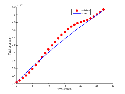
The values of the parameters $\rho=0.1$ and $\gamma=0.33$ are taken from [54] and [5], respectively. It is assumed that after one year, the HIV infected individuals $I$ that are under ART treatment have a low viral load [50] and, therefore, are transferred to class $C$. In agreement, it is taken $\phi=1$. It is well known that taking ART therapy is a long-term commitment. Following [56], it is assumed that the default treatment rate for $C$ individuals is approximately 11 years ($1/\omega$ years, to be precise). The AIDS induced death rate is assumed to be $d=1$ based on [69]. Following the World Bank data [64, 65], the natural death rate is assumed to take the value $\mu=1/69.54$. The recruitment rate $\Lambda=13045$ was estimated in order to approximate the values of the total population of Cape Verde given in Table 2. See Figure 1, were it is observable that model (2) fits well the total population of Cape Verde.

Figure 1: Model (2) fitting the total population of Cape Verde between 1987 and 2014 [52, 65]. The $l_{2}$ norm of the difference between the real total population of Cape Verde and our prediction gives an error of $1.9\%$ of individuals per year with respect to the total population of Cape Verde in 2014 (see [57]).

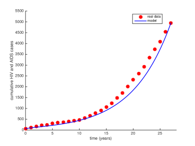
The AIDS induced death rate is assume to be $d=1$ based on [69]. Two cases are considered: $\eta_{C}=0.04$, based on a research study known as HPTN 052, where it is found that the risk of HIV transmission among heterosexual serodiscordant couples is 96% lower when the HIV-positive partner is on treatment [13]; and $\eta_{C}=0.015$, which means that HIV-infected individuals under ART treatment have a very low probability of transmitting HIV, based on [17]. For the modification parameter $\eta_{A}\geq 1$ that accounts for the relative infectiousness of individuals with AIDS symptoms, in comparison to those infected with HIV with no AIDS symptoms, we assume $\eta_{A}=1.3$ and $\eta_{A}=1.35$, based in [63]. We estimated the value of the HIV transmission rate $\beta$ for $(\eta_{C},\eta_{A})=(0.04,1.35)$ equal to $0.695$ and for $(\eta_{C},\eta_{A})=(0.015,1.3)$ equal to $0.752$, and show that model (2) predicts well the reality of Cape Verde for these parameter values: see Figure 2. All the considered parameter values are resumed in Table 3.

(a) $(\beta,\eta_{C},\eta_{A})=(0.752,0.015,1.3)$

(b) $(\beta,\eta_{C},\eta_{A})=(0.695,0.04,1.35)$

Figure 2: Model (2) fitting the data of cumulative cases of HIV and AIDS infection in Cape Verde between 1987 and 2014 [52]. The $l_{2}$ norm of the difference between the real data and the cumulative cases of infection by HIV/AIDS given by model (2) gives, in both cases, an error of $0.03\%$ of individuals per year with respect to the total population of Cape Verde in 2014 (see [57]).

Table 3: Parameter values of HIV/AIDS models (2) and (15) for Cape Verde [57] and Morocco [40].

Symbol	Description	Cape Verde	Morocco	References
$N(0)$	Initial population	$323972$	$23023935$	[64, 66]
$\Lambda$	Recruitment rate	$13045$	$2.19\,\mu$	[64, 51]
$\mu$	Natural death rate	$1/69.54$	$1/74.02$	[64, 51]
$\beta$	HIV transmission rate	$0.752$	$0.755$	[57, 40]
$\eta_{C}$	Modification parameter	$0.015$, $0.04$	$0$	[57]
$\eta_{A}$	Modification parameter	$1.3$, $1.35$	$0$	[57]
$\phi$	HIV treatment rate for $I$ individuals	$1$	$1$	[55, 50]
$\rho$	Default treatment rate for $I$ individuals	$0.1$	$0.1$	[55, 54]
$\gamma$	AIDS treatment rate	$0.33$	$0.33$	[55, 5]
$\omega$	Default treatment rate for $C$ individuals	$0.09$	$0.09$	[55]
$d$	AIDS induced death rate	$1$	$1$	[69]

For the triplets $(\beta,\eta_{C},\eta_{A})=(0.752,0.015,1.3)$ and $(\beta,\eta_{C},\eta_{A})=(0.695,0.04,1.35)$, and the other parameter values from Table 3, we have that the basic reproduction number is given by $R_{0}=4.0983$ and $R_{0}=4.5304$, respectively.

5.2 Particular case $\eta_{A}=\eta_{C}=0$, case study in Morocco (1986–2015)

In [56] and [40], it is assumed that $\eta_{A}=\eta_{C}=0$, based on the assumptions made in Subsection 4.1. Based on these two assumptions, susceptible individuals acquire HIV infection by following effective contact with individuals in the class $I$ at a rate $\lambda=\beta\frac{I}{N}$. Taking into account the data from the Ministry of Health in Morocco [48], in [40] the value of the HIV transmission rate is estimated to be $\beta=0.755$. Moreover, the following initial conditions are considered based on Moroccan data:

$$S_{0}=(N_{0}-(2+9))/N_{0},\quad\ I_{0}=2/N_{0},\quad\ C_{0}=0,\quad\ A_{0}=9/N_{0},$$ (20)

with the initial total population $N_{0}=23023935$ [66]. The values of the parameters $\rho=0.1$, $\phi=1$, $\omega=0.09$ and $d=1$ are the same as the ones used in Subsection 5.1. Following [51], the natural death and recruitment rates are assumed to take the values $\mu=1/74.02$ and $\Lambda=2.19\mu$. All the considered parameter values are summarized in Table 3.

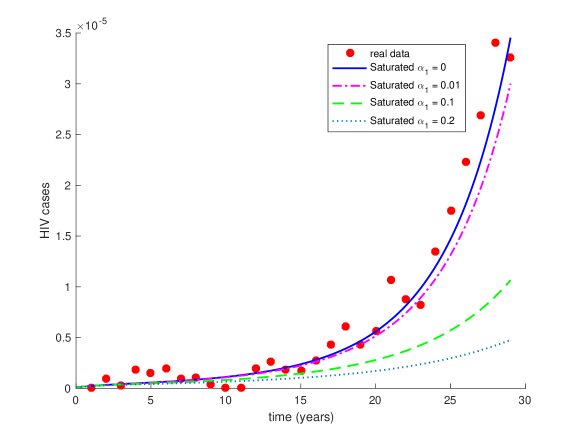
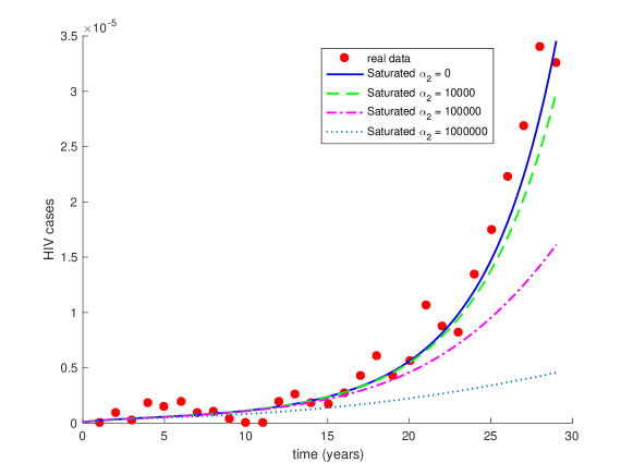
In Figure 3, we observe that model (15) fits the real data reported in [48]. The HIV cases described by model (15) are given by $I(t)+C(t)+\mu\left(I(t)+C(t)\right)$ for $t\in[0,29]$, which corresponds to the interval of time between the years of 1986 ($t=0$) and 2015 ($t=29$).

Figure 3: Model (15) fitting the data of HIV cases in Morocco between 1986 ($t=0$) and 2015 ($t=29$).

For the saturated incidence function $\dfrac{\beta S}{1+\alpha_{1}S}$ [38], see Figure 4.

Figure 4: Saturated incidence function $\dfrac{\beta S}{1+\alpha_{1}S}$ with $\alpha_{1}\in\{0,0.01,0.1,0.2\}$. Time $t=0$ corresponds to the year 1986.

For the saturated incidence function $\dfrac{\beta S}{1+\alpha_{2}I}$ [67], see Figure 5.

Figure 5: Saturated incidence function $\dfrac{\beta S}{1+\alpha_{2}I}$ with $\alpha_{2}\in\{0,10^{4},10^{5},10^{6}\}$. Time $t=0$ corresponds to the year 1986.

For the Beddington–DeAngelis incidence function $\dfrac{\beta S}{1+\alpha_{1}S+\alpha_{2}I}$ [4, 6, 15], see Figure 6.

Figure 6: Beddington–DeAngelis incidence function $\dfrac{\beta S}{1+\alpha_{1}S+\alpha_{2}I}$ with $\alpha_{1}\in\{0,0.01,0.1\}$ and $\alpha_{2}\in\{0,10^{4},10^{5},10^{6}\}$. Time $t=0$ corresponds to the year 1986, see [40].

For the specific non-linear incidence function $\dfrac{\beta S}{1+\alpha_{1}S+\alpha_{2}I+\alpha_{3}SI}$ [27, 28, 31, 41, 47], see Figure 7.

Figure 7: Specific non-linear incidence function $\dfrac{\beta S}{1+\alpha_{1}S+\alpha_{2}I+\alpha_{3}SI}$ with $\alpha_{1}\in\{0,0.1\}$, $\alpha_{2}\in\{0,10^{4},10^{5},10^{6}\}$ and $\alpha_{3}\in\{0,10^{-6},10,10^{2}\}$. Time $t=0$ corresponds to the year 1986, see [40].

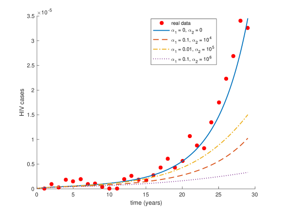
In Tables 4 and 5, the basic reproduction number $R_{0}$ is computed for each incidence function proposed in Table 1 with the parameter values from Table 3, see [40].

Table 4: Basic reproduction number for some special incidence functions, see [40].

Incidence functions	${f(S,I)}$	$R_{0}$
Bilinear	$\beta S$	$7.5340$
Saturated I	$\dfrac{\beta S}{1+\alpha_{1}S}$	$\dfrac{0.0031}{0.0009\,\alpha_{1}+0.0004}$
Saturated II	$\dfrac{\beta S}{1+\alpha_{2}I}$	$7.5340$
Beddington–DeAngelis	$\dfrac{\beta S}{1+\alpha_{1}S+\alpha_{2}I}$	$\dfrac{0.0031}{0.0009\,\alpha_{1}+0.0004}$
Crowley–Martin	$\dfrac{\beta S}{1+\alpha_{1}S+\alpha_{2}I+\alpha_{1}\alpha_{2}SI}$	$\dfrac{0.0031}{0.0009\,\alpha_{1}+0.0004}$
Specific non-linear	$\dfrac{\beta S}{1+\alpha_{1}S+\alpha_{2}I+\alpha_{3}SI}$	$\dfrac{0.0031}{0.0009\,\alpha_{1}+0.0004}$
Hattaf–Yousfi	$\dfrac{\beta S}{\alpha_{0}+\alpha_{1}S+\alpha_{2}I+\alpha_{3}SI}$	$\dfrac{0.0031}{0.0004\,\alpha_{0}+0.0009\,\alpha_{1}}$

Table 5: Basic reproduction number for different values of $\alpha_{1}$ for the incidence function Saturated I, Beddington–DeAngelis, Crowley–Martin and Specific non-linear, see [40].

$\alpha_{1}$	$0.01$	$0.1$	$0.2$
$R_{0}$	$7.3725$	$6.1804$	$5.2392$

In Table 6, we present the sensitivity index of parameters $\beta$, $\phi$, $\rho$, $\gamma$ and $\omega$, computed for the parameter values given in Table 3.

Table 6: Sensitivity index of $R_{0}$ for parameter values given in Table 3 for the bilinear incidence function $f(S,I)=\beta S$, see [40].

Parameter	Sensitivity index
$\beta$	+1
$\phi$	$-0.5947$
$\rho$	$-0.3437$
$\gamma$	$+0.0844$
$\omega$	$+0.5170$

6 Conclusion

We have treated different SICA models for HIV/AIDS transmission: deterministic and stochastic, with integer- and fractional-order derivatives. The superiority or better usefulness of one model over the others depends always on the concrete situation one is studying. For example, let us consider the case study of HIV/AIDS infection in Morocco from 1986 to 2015, and compare the deterministic model (11), both for integer-order ($\alpha=1$) and fractional-order cases ($\alpha\in(0,1)$), with the stochastic model (12). In this case, the results are shown in Figure 8.

Figure 8: Comparison of integer-order, fractional, deterministic and stochastic models, (11) and (12), with $\eta_{A}=\eta_{C}=0$.

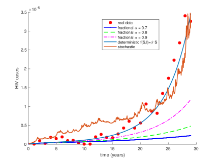
We see that, in this example, the best modeling is obtained using the deterministic model (11) with integer-order derivatives ($\alpha=1$).

All our simulations have been done using the numerical computing environment Matlab, release R2016a, on an Apple MacBook Air Core i5 1.3 GHz with 4Gb RAM. The solutions of the models were found in “real time”. For example, the total computing time needed to generate and plot the 5 solutions in Figure 8, obtained by solving deterministic, stochastic, integer-order and fractional models, was as small as 3.03 seconds.

References

- [1] F. B. Agusto, S. Lenhart, A. B. Gumel and A. Odoi, Mathematical analysis of a model for the transmission dynamics of bovine tuberculosis, Math. Meth. Appl. Sci. 34 (2011), no. 15, 1873–1887.
- [2] E. Ahmed, A.S. Elgazzar, On fractional order differential equations model for nonlocal epidemics, Physica A: Statistical Mechanics and its Applications 379 (2007), no. 2, 607–614.
- [3] R. Almeida, S. Pooseh, D. F. M. Torres, Computational methods in the fractional calculus of variations, Imperial College Press, London, 2015.
- [4] J. R. Beddington, Mutual interference between parasites or predators and its effect on searching efficiency, J. Animal Ecol 44 (1975), 331–341.
- [5] C. P. Bhunu, W. Garira and Z. Mukandavire, Modeling HIV/AIDS and tuberculosis coinfection, Bull. Math. Biol. 71 (2009), no. 7, 1745–1780.
- [6] R. S. Cantrell, C. Cosner, On the dynamics of predator-prey models with the Beddington-DeAngelis functional response, J. Math. Anal. Appl. 257 (2001), no. 1, 206–222.
- [7] V. Capasso, G. Serio, A generalization of the Kermack-McKendrick deterministic epidemic model, Math. Biosci. 42 (1978), no. 1-2, 43–61.
- [8] M. Caputo, Linear models of dissipation whose is almost frequency independent. II, Fract. Calc. Appl. Anal. 11 (2008), no. 1, 4–14.
- [9] J. Carr, Applications centre manifold theory, Springer-Verlag, New-York (1981).
- [10] C. Castillo-Chavez, Z. Feng and W. Huang, On the computation its role on global stability, Mathematical approaches for emerging and re-emerging infectious diseases. IMA, 125 (2002), 229–250.
- [11] C. Castillo-Chavez and B. Song, Dynamical models of tuberculosis and their applications, Math. Biosc. Engrg. 1 (2004), no. 2, 361–404.
- [12] N. Chitnis, J. M. Hyman and J. M. Cushing, Determining important parameters in the spread of malaria through the sensitivity analysis of a mathematical model, Bull. Math. Biol. 70 (2008), no. 5, 1272–1296.
- [13] M. S. Cohen, Y. Q. Chen, M. McCauley et al., Prevention of HIV-1 infection with early antiretroviral therapy, New England Journal of Medicine 365 (2011), no. 6, 493–505.
- [14] P. H. Crowley and E. K. Martin, Functional responses and interference within and between year classes of a dragonfly population, J. North. Am. Benth. Soc. 8 (1989), 211–221.
- [15] D. L. DeAngelis, R. A. Goldstein and R. V. O’Neill, A model for tropic interaction, Ecology 56 (1975), no. 4, 881–892.
- [16] S. G. Deeks, S. R. Lewin, D. V. Havlir, The end of AIDS: HIV infection as a chronic disease, The Lancet 382 (2013), Issue 9903, 1525–1533.
- [17] J. Del Romero, M. B. Baza, I. Río, A. Jerónimo, M. Vera, V. Hernando, C. Rodríguez and J. Castilla, Natural conception in HIV-serodiscordant couples with the infected partner in suppressive antiretroviral therapy: A prospective cohort study, Medicine (Baltimore) 95 (2016), no. 30, e4398.
- [18] H. Delavari, D. Baleanu, J. Sadati, Stability analysis of Caputo fractional-order nonlinear systems revisited, Nonlinear Dynam. 67 (2012), no. 4, 2433–2439.
- [19] K. Diethelm, A. D. Freed, The FracPECE Subroutine for the Numerical Solution of Differential Equations of Fractional Order, in Forschung und Wissenschaftliches Rechnen 1998, Gessellschaft fur Wissenschaftliche Datenverarbeitung, Heinzel, S. and Plesser, T. (1999), 57–71.
- [20] J. Djordjevic, C. J. Silva, D. F. M. Torres, A stochastic SICA epidemic model for HIV transmission, Appl. Math. Lett. 84 (2018), 168–175. arXiv:1805.01425
- [21] R. Garrappa, Predictor-corrector PECE method for fractional differential equations, MATLAB Central File Exchange (2011), File ID: 32918.
- [22] A. J. George, A. Chakrabarti, The Adomian method applied to some extraordinary differential equations, Appl. Math. Lett. 8 (1995), no. 3, 91–97.
- [23] R. Q. Grafton, T. Kompas, D. Lindenmayer, Marine reserves with ecological uncertainty, Bull. Math. Biol. 67 (2005), no. 5, 957–971.
- [24] A. Gray, D. Greenhalgh, L. Hu, A. Mao, J. Pan, A stochastic differential equation SIS epidemic model, SIAM J. Appl. Math. 71 (2011), no. 3, 876–902.
- [25] D. Greenhalgh, Y. Liang, X. Mao, Modelling the effect of telegraph noise in the SIRS epidemic model using Markovian switching, Phys. A 462 (2016), 684–704.
- [26] K. Hattaf, A. A. Lashari, Y. Louartassi and N. Yousfi, A delayed SIR epidemic model with general incidence rate, Electron. J. Qual. Theory Differ. Equ. 2013 (2013), no. 3, 9 pp.
- [27] K. Hattaf, M. Mahrouf, J. Adnani and N. Yousfi, Qualitative analysis of a stochastic epidemic model with specific functional response and temporary immunity, Phys. A 490 (2018), 591–600.
- [28] K. Hattaf and N. Yousfi, Global dynamics of a delay reaction-diffusion model for viral infection with specific functional response, Comput. Appl. Math. 34 (2015), no. 3, 807–818.
- [29] K. Hattaf and N. Yousfi, A class of delayed viral infection models with general incidence rate and adaptive immune response, Int. J. Dyn. Control 4 (2016), no. 3, 254–265.
- [30] K. Hattaf, N. Yousfi and A. Tridane, Mathematical analysis of a virus dynamics model with general incidence rate and cure rate, Nonlinear Anal. Real World Appl. 13 (2012), no. 4, 1866–1872.
- [31] K. Hattaf, N. Yousfi and A. Tridane, Stability analysis of a virus dynamics model with general incidence rate and two delays, Appl. Math. Comput. 221 (2013), 514–521.
- [32] K. Hattaf, N. Yousfi and A. Tridane, A delay virus dynamics model with general incidence rate, Differ. Equ. Dyn. Syst. 22 (2014), no. 2, 181–190.
- [33] C. Ji and D. Jiang, Threshold behaviour of a stochastic SIR model, Appl. Math. Model. 38 (2014), no. 21-22, 5067–5079.
- [34] W. O. Kermack and A. G. McKendrick, Contributions to the mathematical theory of epidemics, part I, Proc. Roy. Soc. Edinburgh A 115 (1927), 700–721.
- [35] A. Lahrouz, L. Omari, Extinction and stationary distribution of a stochastic SIRS epidemic model with non-linear incidence, Statist. Probab. Lett. 83 (2013), no. 4, 960–968.
- [36] J. P. LaSalle, The Stability of Dynamical Systems, SIAM, Philadelphia, PA, 1976.
- [37] Y. Li, Y. Chen, I. Podlubny, Mittag-Leffler stability of fractional order nonlinear dynamic systems, Automatica J. IFAC 45 (2009), no. 8, 1965–1969.
- [38] X. Liu and L. Yang, Stability analysis of an SEIQV epidemic model with saturated incidence rate, Nonlinear Anal. Real World Appl. 13 (2012), no. 6, 2671–2679.
- [39] X.-Q. Liu, S.-M. Zhong, B.-D. Tian and F.-X. Zheng, Asymptotic properties of a stochastic predator-prey model with Crowley-Martin functional response, J. Appl. Math. Comput. 43 (2013), no. 1-2, 479–490.
- [40] E. M. Lotfi, M. Mahrouf, M. Maziane, C. J. Silva, D. F. M. Torres and N. Yousfi, A minimal HIV-AIDS infection model with general incidence rate and application to Morocco data, Stat. Optim. Inf. Comput. 7 (2019), no. 2, 588–603. arXiv:1812.06965
- [41] E. M. Lotfi, M. Maziane, K. Hattaf and N. Yousfi, Partial differential equations of an epidemic model with spatial diffusion, Int. J. Partial Differ. Equ. 2014 (2014), Art. ID 186437, 6 pp.
- [42] E. M. Lotfi, M. Maziane, M. Mahrouf, K. Hattaf and N. Yousfi, Global stability of a diffused SIR epidemic model with general incidence rate and time delay, Int. J. Math. Anal. (Ruse) 10 (2016), no. 17, 807–816.
- [43] Q. Lu, Stability of SIRS system with random perturbations, Phys. A 388 (2009), no. 18, 3677–3686.
- [44] M. Mahrouf, K. Hattaf and N. Yousfi, Dynamics of a stochastic viral infection model with immune response, Math. Model. Nat. Phenom. 12 (2017), no. 5, 15–32.
- [45] D. Matignon, Stability Results For Fractional Differential Equations With Applications To Control Processing, in Computational Engineering in Systems Applications (1996), 963–968.
- [46] R. M. May, R. M. Anderson, Transmission dynamics of HIV infection, Nature 326 (1987), 137–142.
- [47] M. Maziane, E. M. Lotfi, K. Hattaf and N. Yousfi, Dynamics of a class of HIV infection models with cure of infected cells in eclipse stage, Acta Biotheoretica 63 (2015), no. 4, 363–380.
- [48] Ministry of Health, Morocco, Department of Epidemiology and Disease Control, http://www.sante.gov.ma/Pages/Accueil.aspx
- [49] K. M. Owolabi, A. Atangana, Spatiotemporal Dynamics of Fractional Predator–Prey System with Stage Structure for the Predator, Int. J. Appl. Comput. Math. 3 (2017), 903–924.
- [50] A. S. Perelson, P. Essunger, Y. Cao, M. Vesanen, A. Hurley, K. Saksela, M. Markowitz and D. D. Ho, Decay characteristics of HIV-1-infected compartments during combination therapy, Nature 387 (1997), 188–191.
- [51] Population Data, Maroc, http://www.populationdata.net/pays/maroc
- [52] República de Cabo Verde, Rapport de Progrès sur la riposte au SIDA au Cabo Verde – 2015, Comité de Coordenação do Combate a Sida, 2015.
- [53] H. S. Rodrigues, M. T. T. Monteiro and D. F. M. Torres, Sensitivity analysis in a dengue epidemiological model, Conf. Papers in Math. 2013 (2013), Art. ID 721406, 7 pp. arXiv:1307.0202
- [54] O. Sharomi, C. N. Podder, A. B. Gumel and B. Song, Mathematical analysis of the transmission dynamics of HIV/TB coinfection in the presence of treatment, Math. Biosci. Eng. 5 (2008), no. 1, 145–174.
- [55] C. J. Silva and D. F. M. Torres, A TB-HIV/AIDS coinfection model and optimal control treatment, Discrete Contin. Dyn. Syst. 35 (2015), no. 9, 4639–4663. arXiv:1501.03322
- [56] C. J. Silva and D. F. M. Torres, A SICA compartmental model in epidemiology with application to HIV/AIDS in Cape Verde, Ecological Complexity, 30 (2017) 70–75. arXiv:1612.00732
- [57] C. J. Silva and D. F. M. Torres, Modeling and optimal control of HIV/AIDS prevention through PrEP, Discrete Contin. Dyn. Syst. Ser. S 11 (2018), no. 1, 119–141. arXiv:1703.06446
- [58] C. J. Silva and D. F. M. Torres, Stability of a fractional HIV/AIDS model, Math. Comput. Simul. 164 (2019), 180–190. arXiv:1903.02534
- [59] E. Tornatore, S. M. Buccellato, On a stochastic SIR model, Applicationes Mathematicae 34 (2007), no. 4, 389–400.
- [60] P. van den Driessche and J. Watmough, Reproduction numbers and subthreshold endemic equilibria for compartmental models of disease transmission, Math. Biosc. 180 (2002), 29–48.
- [61] C. Vargas-De-León, Cruz, Volterra-type Lyapunov functions for fractional-order epidemic systems, Commun. Nonlinear Sci. Numer. Simul. 24 (2015), no. 1-3, 75–85.
- [62] J.-J. Wang, J.-Z. Zhang and Z. Jin, Analysis of an SIR model with bilinear incidence rate, Nonlinear Anal. Real World Appl. 11 (2010), no. 4, 2390–2402.
- [63] D. P. Wilson, M. G. Law, A. E. Grulich, D. A. Cooper and J. M. Kaldor, Relation between HIV viral load and infectiousness: A model-based analysis, The Lancet 372 (2008), no. 9635, 314–320.
- [64] World Bank Data, Cabo Verde, World Development Indicators, http://data.worldbank.org/country/cape-verde
- [65] World Bank Data, Population, total – Cabo Verde http://data.worldbank.org/indicator/SP.POP.TOTL?locations=CV
- [66] World Bank Data, Morocco, http://data.worldbank.org/country/morocco
- [67] Y. Zhao, D. Jiang, The threshold of a stochastic SIRS epidemic model with saturated incidence, Appl. Math. Lett. 34 (2014), 90–93.
- [68] X. Zhou and J. Cui, Global stability of the viral dynamics with Crowley-Martin functional response, Bull. Korean Math. Soc. 48 (2011), no. 3, 555–574.
- [69] M. Zwahlen and M. Egger, Progression and mortality of untreated HIV-positive individuals living in resource-limited settings: Update of literature review and evidence synthesis, Report on UNAIDS obligation no. HQ/05/422204, 2006.