Application of Progressive Hedging to Var Expansion Planning Under Uncertainty

Abstract

This paper describes the application of a Progressive Hedging (PH) algorithm to the least-cost var planning under uncertainty. The method PH is a scenario-based decomposition technique for solving stochastic programs, i.e., it decomposes a large scale stochastic problem into s deterministic subproblems and couples the decision from the s subproblems to form a solution for the original stochastic problem. The effectiveness and computational performance of the proposed methodology will be illustrated with var planning studies for the IEEE 24-bus system (5 operating scenarios), the 200-bus Bolivian system (1,152 operating scenarios) and the 1,600-bus Colombian system (180 scenarios).

1 Introduction

The fast worldwide insertion of variable renewable energy (VRE) sources such as wind and solar has brought substantial economic and environmental benefits. However, it has also created some technical challenges, for instance, the need for additional generation reserve and/or storage to manage the VRE intermittency. In many systems, VRE sources also disrupted the usual power flow patterns (around which the transmission networks were designed), creating congestions and voltage issues. The solution of these network problems may require substantial investments in new lines, FACTS devices and var sources. Due to the complexity of real networks (size, nonconvexity, discrete variables, uncertainty on load and generator production etc.), transmission planners usually apply a two-step hierarchical approach.

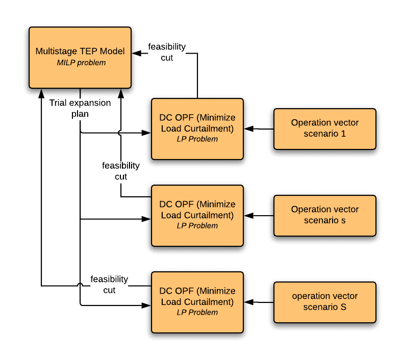
The first step determines the least-cost reinforcements of circuits and transformers that eliminate overloads for many operational scenarios (robust optimization). This planning step uses a linearized active optimal power flow (OPF) representation. Because the linearized OPF is convex, it is also possible to use Benders decomposition latorre2019stochasticrobust to handle the multiple operational scenarios (see Fig. 1).

Figure 1: First step of the planning process – circuit/transformer reinforcements (Benders decomposition). Source: latorre2019stochasticrobust

Given the active power reinforcements from the first step, the second step - which is the focus of this paper - determines the least cost var reinforcements ensuring that voltage levels remain within their limits for the same set of operational scenarios used previously vaahedi2001dynamic . This var planning step is arguably more challenging than the first step for two reasons: (i) it requires the solution of AC OPFs, which are nonlinear nonconvex optimization problems; (ii) because of nonconvexities, many decomposition techniques cannot be directly applied.

This paper describes the application of a Progressive Hedging (PH) algorithm wets1989aggregation to the least-cost var planning under uncertainty. Similarly to Benders decomposition benders1962partitioning , PH is based on the separate solutions of AC OPF granville1988integrated subproblems for each scenario. The difference is that, instead of an investment module, there is an update in the OPF objective functions. The PH has already been applied successfully to other related problems such as unit commitment ryan2013toward ; gade2016obtaining , transmission and generation planning munoz2015scalable , and a dynamic deterministic OPF ruppert2018dynamic , but to the best of our knowledge, it has not been applied yet to the stochastic var expansion problem.

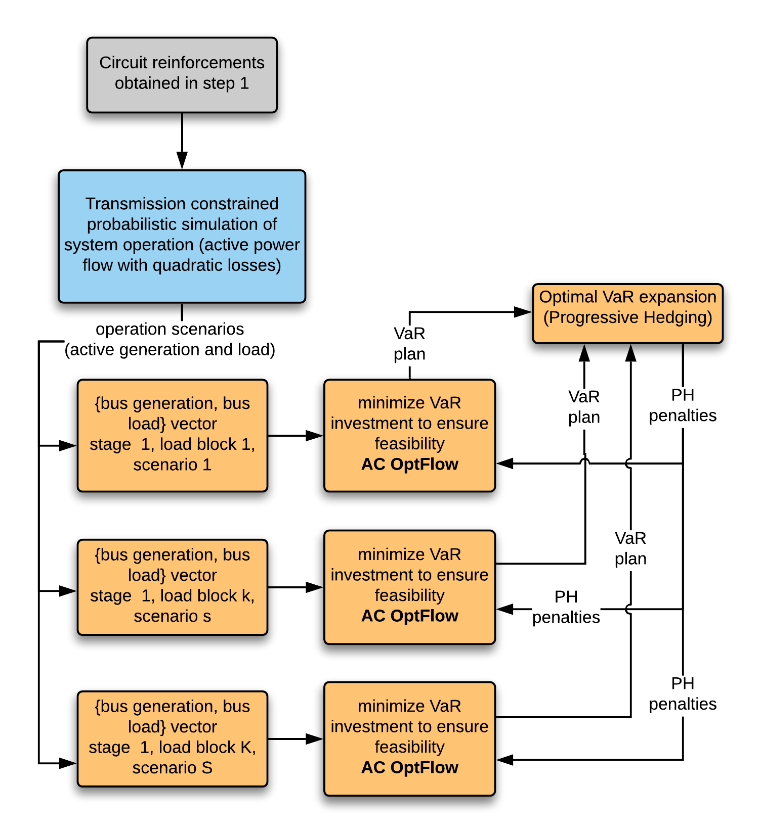
Although global optimality cannot be guaranteed in the case of nonconvex subproblems, PH has attracted our interest for the following reasons: (i) it is straightforward to implement; (ii) each subproblem is a (slightly modified) OPF, which can be solved by effective techniques such as nonlinear interior point methods granville1994optimal ; (iii) the OPF subproblems can be solved in parallel; (iv) it has recently become possible to calculate lower bounds to the optimal solution through convex relaxations; and (v) as will be illustrated in this paper, the resulting var plans are near-optimal. Fig. 2 shows the proposed PH scheme.

Figure 2: PH procedure for var planning under uncertainty.

The proposed algorithm is be detailed described in Section 2. Then we present a case study in Section 3, where the methodology is initially illustrated for the IEEE 24-bus test case, and then applied to realistic studies of the Bolivian and Colombian power systems. Finally, conclusions are drawn in Section 4.

2 Progressive Hedging Algorithm

The PH scheme is implemented in the following steps:

1. Initialize the PH linear and quadratic terms

2. Solve the modified OPF problems for scenarios $s\in 1,\dots,S$. For completeness, we highlight the non-linear OPF model:

   Objective function:

   $$\min \sum_{k}[I_{k}^{R}Q_{k,(s)}^{C,INV}+I_{k}^{C}Q_{k,(s)}^{C,INV}$$ (1)

   $$+w_{k,(s)}^{R}(Q_{k,(s)}^{R,INV}-Q_{k}^{R,AVE})+w_{k,(s)}^{C}(Q_{k,(s)}^{C,INV}-Q_{k)}^{C,AVE})$$ (2)

   $$+\rho_{k}^{R}(Q_{k,(s)}^{R,INV}-Q_{k}^{R,AVE})^{2}/2+\rho_{k}^{C}(Q_{k,(s)}^{C,INV}-Q_{k}^{C,AVE})^{2}/2]$$ (3)

   where:

   $I_{k}^{R}$ and $I_{k}^{C}$ are, respectively, the unit investment costs ($/Mvar) of reactor and capacitor banks in bus k;

   $Q_{k,(s)}^{R,INV}$ and $Q_{k,(s)}^{C,INV}$ are the investment decisions: reactor and capacitor sizes (Mvar) for each scenario s.;

   $w_{k,(s)}^{R}$ and $w_{k,(s)}^{C}$ are the weights of the linear PH terms;

   $\rho_{k}^{R}$ and $\rho_{k}^{R}$ are the weights of the quadratic PH terms.

   As seen in the equation above, the PH terms are related to the linear and quadratic differences between the var investment decisions for each scenario $s$, $Q_{k,(s)}^{R,INV}$ and $Q_{k,(s)}^{C,INV}$, and “target” investments $Q_{k)}^{R,AVE}$ and $Q_{k}^{C,AVE}$ (known values).

   Capacity limits on var injections:

   $$0\leq Q_{k,(s)}^{R,INJ}\leq Q_{k,(s)}^{R,INV}$$ (4)

   $$0\leq Q_{k,(s)}^{C,INJ}\leq Q_{k,(s)}^{C,INV}$$ (5)

   where $Q_{k,(s)}^{R,INJ}$ and $Q_{k,(s)}^{R,INJ}$ are the operational decisions. They are the decision variables to choose how much power will be injected in each bus $k$ for each scenario $s$. They are limited by how much was invested.

   AC power flow equations and constraints:

   $$P_{k,(s)}^{GEN}-P_{k,(s)}^{DEM}-\sum_{j\in\Omega_{k}}P_{k,j,(s)}^{FLW}(v_{k},v_{j},\theta_{k},\theta_{j},t_{k,j},\phi_{k,j})=0$$ (6)

   $$Q_{k,(s)}^{GEN}-Q_{k,(s)}^{DEM}-\sum_{j\in\Omega_{k}}Q_{k,j,(s)}^{FLW}(v_{k},v_{j},\theta_{k},\theta_{j},t_{k,j},\phi_{k,j})+Q_{k,(s)}^{C,INJ}-Q_{k,(s)}^{R,INJ}=0$$ (7)

   $$\sqrt{{P_{k,j,(s)}^{FLW}}^{2}+{Q_{k,j,(s)}^{FLW}}^{2}}\leq\bar{S}_{k,j}$$ (8)

   Variable bounds:

   $$\underline{Q}_{k,(s)}^{GEN} \leq Q_{k,(s)}^{GEN}\leq\bar{Q}_{k,(s)}^{GEN}$$ (9)

   $$\underline{v}_{k} \leq v_{k}\leq\bar{v}_{k}$$ (10)

   $$\underline{t}_{k} \leq t_{k}\leq\bar{t}_{k}$$ (11)

   $$\underline{\phi}_{k} \leq\phi_{k}\leq\bar{\phi}_{k}$$ (12)

   where:

   $P_{k,(s)}^{GEN}$ is the active power generation at bus $k$ (known value, taken from the probabilistic simulation of system operation for scenario $s$, see Fig. 2);

   $Q_{k,(s)}^{GEN}$, reactive power generation at k (decision variable, with limits $\underline{Q}_{k,(s)}^{GEN}$ and $\bar{Q}_{k,(s)}^{GEN}$);

   $P_{k,(s)}^{DEM}$ and $P_{k,(s)}^{DEM}$ active and reactive loads at bus k, also known values, taken from the same simulation;

   $P_{k,j,(s)}^{FLW}$ and $Q_{k,j,(s)}^{FLW}$ active and reactive power flows in circuit k-j, with limit $\bar{S}_{k,j}$;

   $\theta_{k}$ and $\theta_{j}$ voltage angles at buses $k$ and $j$;

   $t_{kj}$, tap position value for transformer $k-j$;

   $v_{k}$, voltage at bus $k$, with limits $\bar{v}_{k}$ and $\underline{v}_{k}$;

   $\phi_{kj}$ phase shifting angle in circuit $k-j$, with limits $\bar{\phi}_{kj}$ and $\underline{\phi}_{kj}$;

3. Let $\{(\tilde{q}_{k}^{rs},\tilde{q}_{k}^{cs}),k\in 1,\dots,K\}$ for $s\in 1,\dots,S$ be the optimal solutions of the modified OPF problems of step (b); carry out the following updates:

   $$Q_{k}^{R,AVE}\leftarrow\sum_{s}Pr(s)Q_{k,(s)}^{R,INV}$$ (13)

   $$Q_{k}^{C,AVE}\leftarrow\sum_{s}Pr(s)Q_{k,(s)}^{C,INV}$$ (14)

   $$w_{k,(s)}^{R}\leftarrow w_{k,(s)}^{R}+\delta_{k)}^{R}\rho_{k}^{r}(Q_{k,(s)}^{R,INV}-Q_{k}^{R,AVE})$$ (15)

   $$w_{k,(s)}^{C}\leftarrow w_{k,(s)}^{C}+\delta_{k)}^{C}\rho_{k}^{r}(Q_{k,(s)}^{C,INV}-Q_{k}^{C,AVE})$$ (16)

   where $\delta_{k)}^{R}$ and $\delta_{k)}^{C}$ are user-defined step sizes, and $Pr(s)$ is vector of the occurrenc probability of each scenario s. It is important to highlight that this step size is a contribution to this paper since the standard PH use an implicit step fixed at 1. In the present work, all scenarios were considered as equiprobable. If the probabilities of the scenarios were different, the method would work in the same way, where the difference consists of the decision variables tending to the value resulting from the weighted average with different weights.

4. In case of convergence, stop; otherwise go to (b).

2.1 Penalty Values Calculations

The PH performance is based on the chosen values for $\rho_{k}^{R}$ and $\rho_{k}^{C}$. With larger values, convergence is faster; on the other hand, there may be an oscillatory behavior. Conversely, smaller values lead to a steadier, but slower, convergence. In this work, $\rho_{k}^{R}$ and $\rho_{k}^{C}$ were made proportional to the respective investment costs $I_{k}^{R}$ and $I_{k}^{C}$.

$$\rho_{k}^{R}=K\cdot I_{k}^{R}$$ (17)

$$\rho_{k}^{C}=K\cdot I_{k}^{C}$$ (18)

where $K$ is a constant chosen to implement variations on the penalty value for each simulation.

2.2 Convergence

Two methods are used to measure convergence in this paper. The first one is the usage of a normalized average per-scenario deviation (NApSD) watson2011progressive from the reference value detects the proximity to the standard convergence of the method:

$$NApSD_{(i)}^{R}=\frac{1}{s}\sum_{k,s|Q_{k}^{R,AVE}>0}\frac{|Q_{k,(s),(i)}^{R,INV}-Q_{k,(i-1)}^{R,AVE}|}{Q_{k,(i-1)}^{R,AVE}}$$ (19)

$$NApSD_{(i)}^{C}=\frac{1}{s}\sum_{k,s|Q_{k,(i-1)}^{C,AVE}>0}\frac{|Q_{k,(s),(i)}^{C,INV}-Q_{k,(i-1)}^{C,AVE}|}{Q_{k,(i-1)}^{C,AVE}}$$ (20)

The NApSD is calculated for each decision variable and varies at each iteration. Note that the index $i$ indicates the iteration and $i-1$ the previously iteration. As shown above, the NApSD is the average of the relative differences between the investment for scenario $s$ and the average of the investments from the previous iteration. The second method to detect convergence is a relative duality gap computed with valid upper ($UB$) and lower bounds ($LB$). The duality gap is defined as $\frac{UB-LB}{UB}$.

The upper bound is constructed by the union of the investments of all scenarios since an over investment does not harm feasibility. Moreover, Gade et al. gade2016obtaining showed how to obtain a lower bound using the PH that is equivalent to the bound provided by the Lagrangian relaxation of the problem that we use in this paper. Since the problem is nonconvex, a zero duality gap could be assured only in special cases lavaei2011zero . The average of these problems is equivalent to a Lagrangian relaxation of the full space problem, thus, generating a lower bound (LB). There are alternative methods to obtain a LB, such as boland2018combining . The method described in gade2016obtaining was implemented since it is simpler. The LB is obtained by solving the PH problem replacing the objective function by the following expression and taking the average for all scenarios.

$$\min \sum_{k}[I_{k}^{R}Q_{k,(s)}^{C,INV}+I_{k}^{C}Q_{k,(s)}^{C,INV}$$ (21)

$$+w_{k,(s)}^{R}(Q_{k,(s)}^{R,INV}-Q_{k}^{R,AVE})+w_{k,(s)}^{C}(Q_{k,(s)}^{C,INV}-Q_{k}^{C,AVE})]$$ (22)

Two additional stop criteria were also considered. The first one consists on verifying the OPF’s convergence for all scenarios under analysis. If any OPF has not converged, the iterative process must stop. The model checks information from the solver if each one of the OPFs has converged or not at each iteration of the method. The other one is for exceeding the maximum number of iterations as established before the method’s execution (timeout). The analysis of simulations with the system is required before defining a good value for this parameter.

3 Case study

The present research considers the application of the methodology described for the IEEE 24-bus test case (10 simulations), and also for the electrical power systems from two southamerican countries: Bolivia (5 simulations) and Colombia (1 simulation).

PSR’s software Optflow optflowmanual was used to run the optimal power flow simulations and served as a basis for the PH implementation. The OptFlow model is based on the primal-dual interior point algorithm granville1994optimal , which have recognized efficiency to solve non convex problems with a large number of variables and constraints. The computer used to run the 10 simulations for the present work consists of an Intel® Core ™ i7-7700K CPU 4.20 GHz with 64 GB of installed RAM.

Artelys Knitro nocedal2006knitro is the local nonlinear solver chosen to obtain the solutions from the OPF previously presented. It solves nonlinear problems by considering integer or continuous variables and is prepared for multiple objective functions and nonlinear constraints.

Since the continuous problem is already complex to solve due to its nonconvexity, we avoided including integer variables into the model. The required investment is decided by choosing how much Mvar is needed at each bus of the system. After the continuous problem is solved, a post-processing is done to choose which shunt equipment should be installed with predetermined capacities and costs.

The list of candidate buses was previously obtained from a process of shunt allocation. Initially, the model is used to identify candidate buses for reactive support, minimizing the reactive power injections in the system, where we discover which buses are in need of reactive support. Results from simulations with IEEE 24-Bus case illustrated the importance of this step.

The cost considered for each var equipment came from a report from Ente Operador Regional (EOR) eor . The values considered are illustrated in Table 1.

Table 1: Var sources cost

Equipament	Cost [kUS$]
5 Mvar Capacitor	313
10 Mvar Capacitor	362
15 Mvar Capacitor	418
15 Mvar Reactor	1,810
60 Mvar Reactor	2,171
Connection Bay	3,217

3.1 IEEE 24-Bus System

The system consists of:

• 24 buses (18 with load, 10 with generating units);

• 50 transmission lines;

• 7 transformers

The list of parameters considered for simulations with the present system is:

• Maximum shunt allocation for each bus: 500 Mvar;

• 5 different generation/load set-points considered at each iteration;

• Maximum number of iterations: 100;

• Convergence gap: 1%

With the IEEE 24-Bus database, the first two simulations were done considering ($\delta_{k}^{rs}$,$\delta_{k}^{cs}$) = 0 and K = 1:

• Simulation 1: Reactive investment is allowed at all buses from the system (Full set of shunt candidates);

• Simulation 2: Reactive investment is allowed only at the buses that presented reactive investment in iteration 0 (Reduced set of shunt candidates)

The comparison of the reactive requirement between these two simulations is presented in Fig. 3.

Figure 3: Mvar requirement reduction for simulations 1 and 2

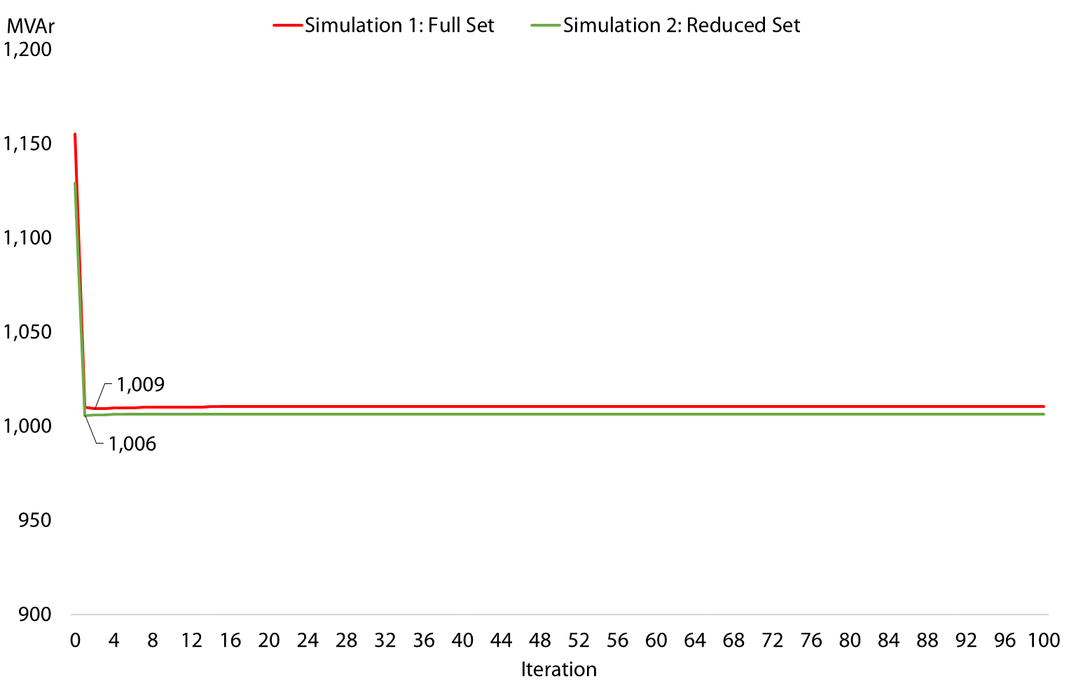
It is observed in the Fig. 3 that, with the reduced set of candidates, the total amount of shunt requirement reaches slightly smaller values than those from Simulation 1. As the results presented were better for the simulations with a reduced set of candidates, for the next simulations presented in this paper, this reduced set will always be considered.

In order to evaluate the impact of the step-size, four more simulations were done with K=1. The set to compare now is:

• Simulation 2: ($\delta_{k}^{rs}$,$\delta_{k}^{cs}$) = 0;

• Simulation 3: ($\delta_{k}^{rs}$,$\delta_{k}^{cs}$) = 0.001;

• Simulation 4: ($\delta_{k}^{rs}$,$\delta_{k}^{cs}$) = 0.01;

• Simulation 5: ($\delta_{k}^{rs}$,$\delta_{k}^{cs}$) = 0.1;

• Simulation 6: ($\delta_{k}^{rs}$,$\delta_{k}^{cs}$) = 1;

The comparison of the total system’s reactive requirement along the iterative process for the five simulations above is illustrated in Fig. 4. It is observed that for Simulation 5 and Simulation 6 (step-sizes 0.1 and 1, respectively), the problem becomes maximizing instead of minimizing in the early first iterations. It occurs because the linear term in the objective function becomes negative in such a way that all objective function becomes negative. Then all reactive investment possible (4,000 MVAr) is allocated. For better comparison between the simulations from this set, Simulation 5 and Simulation 6 were both excluded from Fig. 4.

Figure 4: Mvar requirement reduction for simulations 2-6

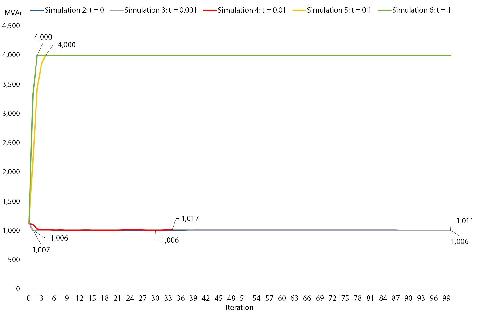
Fig. 5 illustrates the simulations which reduced the system’s requirement from iteration zero. It is observed that Simulation 4 stops before the timeout, because it converges from the duality gap criterium, as illustrated in Fig. 6.

Figure 5: Mvar requirement reduction for simulations 2-4

Figure 6: LB-UB Convergence scheme – IEE 24-Bus.

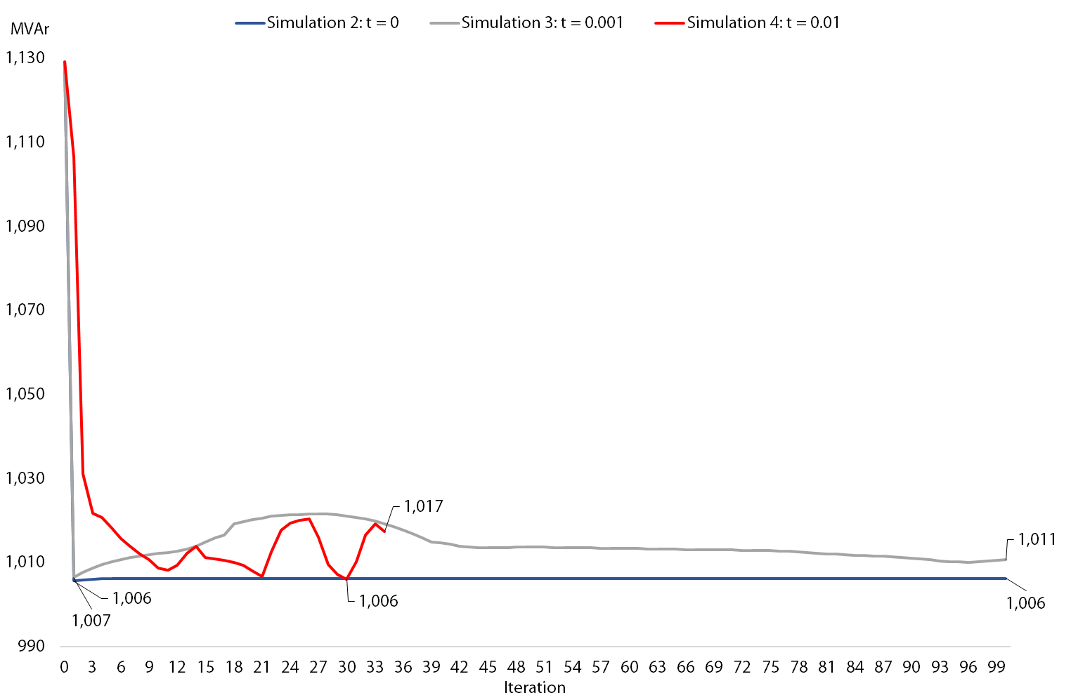
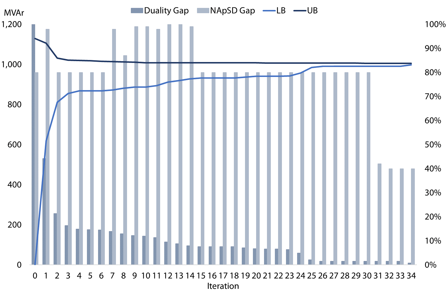
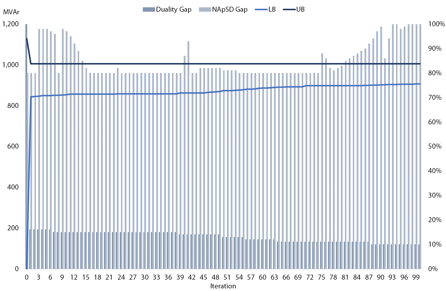
Note that using duality criterion convergence is reached (1% duality gap) while the NApSD criterion is 40% as illustrated in Fig. 6. Simulation 4 converges from the duality gap, and Simulation 2 does not converge from NApSD. As step-size is null at Simulation 2, it is not possible to compute lower bounds, and therefore, the duality gap is not applicable for this simulation. About Simulation 3, the convergence is slower, as illustrated in Fig. 7, and it is concluded that this step-size is, on the other hand, too small.

Figure 7: LB-UB Convergence scheme – IEE 24-Bus.

From the previous analyses, it is concluded that the step-size equals to 0.01 is the best option to proceed with further simulations and analyses. However, to reinforce the idea, the same analyses with the step size parameter will be repeated with the Bolivian system in the next section.

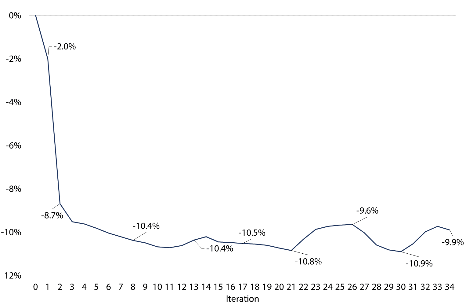
Fig. 8 highlights the reductions on total amount invested compared to the solution obtained without PH (iteration 0). Some oscillatory behavior is observed from variations with weights at each iteration. It is essential to highlight that all solutions are feasible ones, and at the end of the process, the one with the smallest total system’s var requirement is chosen.

Figure 8: Reduction in objective function, Simulation 4– IEEE 24-Bus

In order to evaluate the impact of the penalty parameter, four more simulations were done with ($\delta_{k}^{rs}$,$\delta_{k}^{cs}$) = 0.01. The set to compare now is:

• Simulation 4: K = 1;

• Simulation 7: K = 0.5;

• Simulation 8: K = 2;

• Simulation 9: K = 5;

• Simulation 10: K = 10;

The comparison of the best total system’s reactive requirement found so far along the iterative process for the five simulations above is illustrated in Fig. 9. It is observed that K = 0.5 or 1 results in similar total system’s var requirement. As the constant K rise from 1 to 5, the local optimal solution found is slightly better. The final solution obtained from simulations 11 and 12 (K = 5 and K = 10, respectively) were also similar.

Figure 9: Mvar requirement reduction for simulations 4, 7-10

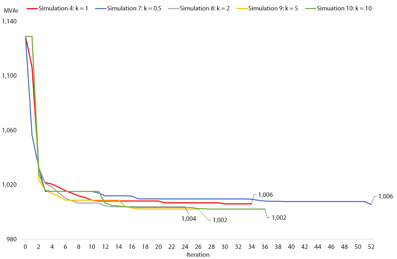
Table 2 summarizes the total CPU time for the whole iterative process from the 10 simulations analyzed for this system.

Table 2: Total CPU Time - IEEE 24 Bus

Simulation	Candidates	t	K	Number of iterations	Total var requirement	CPU Time [min]
1	Full set	0	1	100	1,009	4.1
2	Reduced set	0	1	100	1,006	4.1
3	Reduced set	0.001	1	100	1,007	8.3
4	Reduced set	0.01	1	34	1,006	2.8
5	Reduced set	0.1	1	100	1,129	8.1
6	Reduced set	1	1	100	1,129	8.1
7	Reduced set	0.01	0.5	52	1,006	4.3
8	Reduced set	0.01	2	24	1,004	2.0
9	Reduced set	0.01	5	26	1,002	2.1
10	Reduced set	0.01	10	36	1,002	3.0

From Table 2 it is observed that considering a full set or a reduced set of candidates makes no visible change in computational effort. It is also observed that with the introduction of the step size, the CPU time after 100 iterations doubles. It happens because another problem is required to be solved to compute lower bounds from the duality gap. Then, with a step size different than zero, two problems are solved at each iteration. With the null step size, only one problem is solved, which explains the rise in the CPU time observed in Table 2. The simulations considering a value different than zero for the step-size which presented a CPU time much lower than the others, it is because it has converged from the duality gap criterium in the iteration indicated. It is also observable that the value of the penalty parameter seems to have no interference in the CPU Time required to solve the problem with the method’s application.

3.2 Bolivian Electrical Power System

System overview:

• 215 buses;

• 184 transmission lines;

• 59 transformers;

• 135 generating units;

• 14 shunt equipment

The list of parameters considered for simulations with the present system is:

• Maximum shunt allocation for each bus: 500 Mvar;

• 1,152 different generation/load set-points considered at each iteration;

• Maximum number of iterations: 30;

• Convergence gap: 1%

With the Bolivian system database, two sets of simulations were done in order to evaluate the impact of the step-size and the penalty parameter, as previously done with the IEEE 24-bus system. Then, as stated before, all simulations with the Bolivian system considered a reduced set of shunt candidates. First, in order to evaluate the impact of the step-size, three simulations were done with K=1. The set to compare now is:

• Simulation 11: ($\delta_{k}^{rs}$,$\delta_{k}^{cs}$) = 0.005;

• Simulation 12: ($\delta_{k}^{rs}$,$\delta_{k}^{cs}$) = 0.01;

• Simulation 13: ($\delta_{k}^{rs}$,$\delta_{k}^{cs}$) = 0.1;

The comparison of the reactive requirement between these three simulations is presented in Fig. 10.

Figure 10: Mvar requirement reduction in % for simulations 11-13 – Bolivia

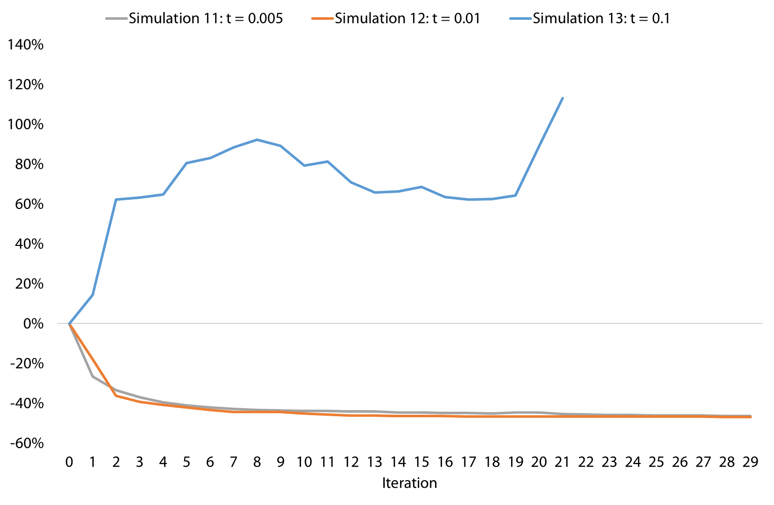
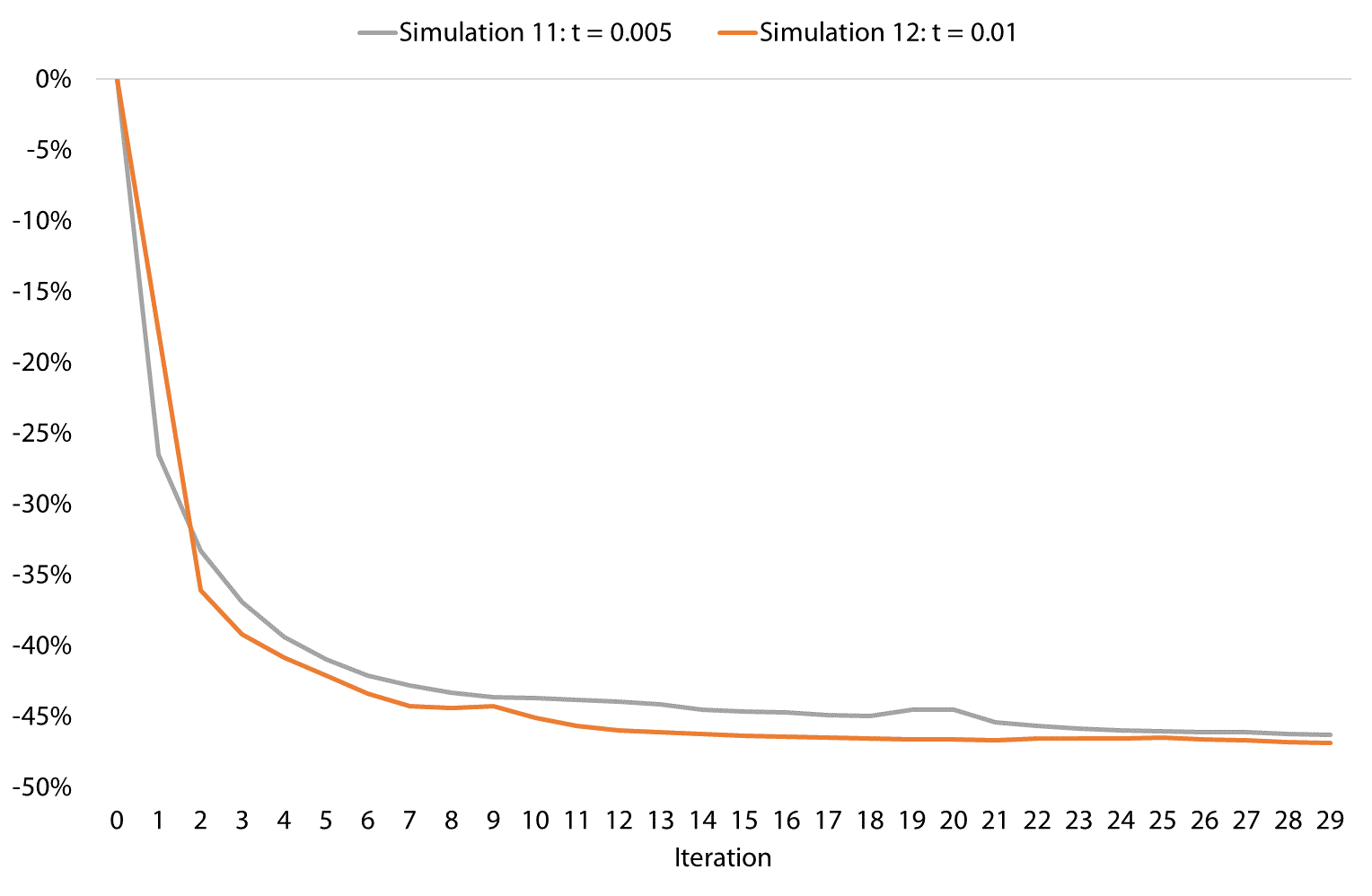
It is observed in Fig. 10 that with a larger step-size (Simulation 13), the weight vectors become negative and higher than the cost in absolute value. It turns the objective function to maximize instead of minimizing the investment in shunt equipment, as observed in the analyses with IEEE 24 bus system. For better comparison, Simulation 13 was excluded from the Fig. 10, and the “simulations with minimization” are illustrated in Fig. 11. It is observed that the smaller step-sizes used for Simulation 11 and Simulation 12 resulted in quite similar amount reductions, where the step-size of 0.01 from Simulation 12 presented slightly better results.

Figure 11: Mvar requirement reduction in % for simulations 11-12 – Bolivia

In the first iterations of the method, great reductions on the total system’s var requirement are obtained. Fig. 12 illustrates the reductions on total amount invested along the iterative process compared to the solution without progressive hedging (iteration 0) for Simulation 12.

Figure 12: Reductions in objective function – Bolivia

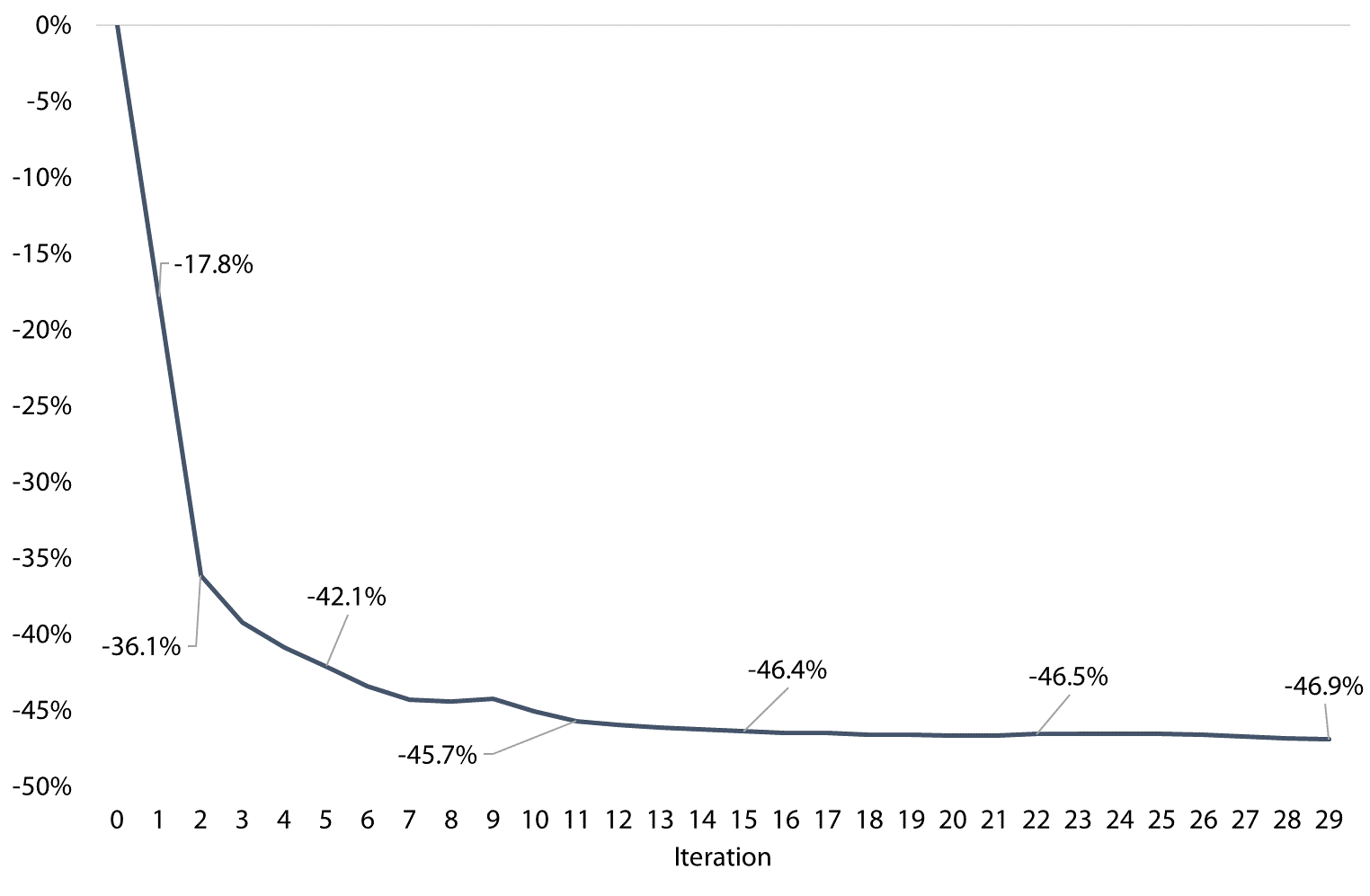
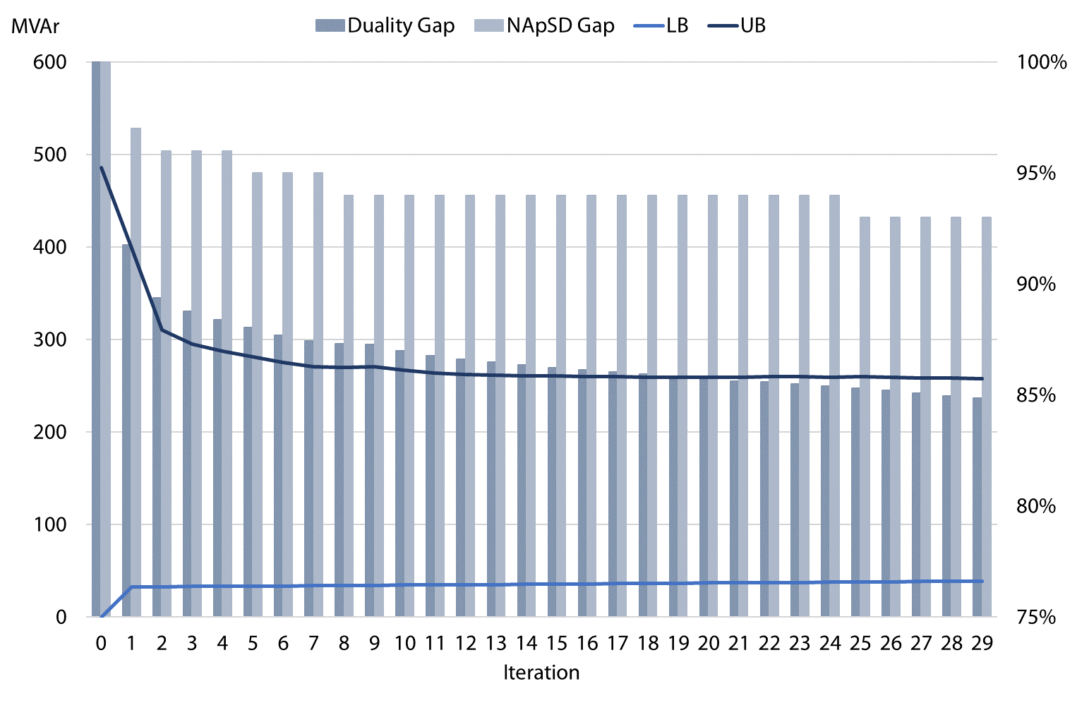
Fig. 13 illustrates the convergence of Simulation 12. Note that duality gap is 85% while the NApSD criterion is 93%. The approximation between LB and UB are very slow, which wait for convergence would take days of simulation, if it reaches convergence. An approach to accelerate the process aiming the convergence is the parallelization of the simulations or better, the clusterization of the 1,152 operative scenarios considered, reducing the number of scenarios to be solved at each iteration.

Figure 13: LB-UB Convergence scheme – Bolivia

In order to evaluate the impact of the penalty parameter, two more simulations were done with ($\delta_{k}^{rs}$,$\delta_{k}^{cs}$) = 0.01. The set to compare now is:

• Simulation 12: K = 1;

• Simulation 14: K = 0.5;

• Simulation 15: K = 2;

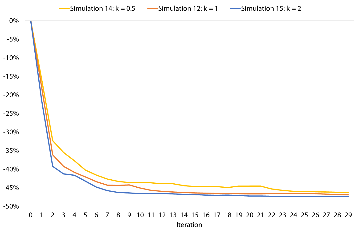
The comparison of the reactive requirement between these three simulations is presented in Fig. 14. It is observed that as the parameter K grows, the more significant is the reduction in the total amount of var required for the first iterations. However, the three simulations seem to stabilize in the same “reduction amount” by the end of the iterative process.

Figure 14: Mvar requirement reduction in % for simulations 12, 14 and 15 – Bolivia

The Table 3 summarizes the total CPU time for the whole iterative process from the 5 simulations analyzed for this system. It is observed that all simulations took basically the same computational effort and stopped by the timeout criterium, except Simulation 13, which stopped before 30 iterations because one of the OPFs in the 23rd iteration did not converge. As the number of iterations rise, the CPU time rises as expected, and compared to the simulations with the IEEE 24-Bus, it is observable that the rise in number of scenarios and size of the system makes the total CPU time to rise. 30 iterations for 5 scenarios with the IEEE 24-Bus system took something between 2 and 3 minutes and here takes more than 10 hours. It is also observable that varying the step-size and k seems to have no interference in the CPU Time required to solve the problem with the method’s application.

Table 3: Total CPU Time - Bolivian system

Simulation	t	k	Number of iterations	Total var requirement	CPU Time [min]
11	0.005	1	30	261	634
12	0.01	1	30	258	638
13	0.1	1	22	486	459
14	0.01	0.5	30	261	637
15	0.01	2	30	256	635

3.3 Colombian Electrical Power System

The system consists of:

• 1,674 buses;

• 1,147 transmission lines;

• 1,179 transformers;

• 388 generating units;

The list of parameters considered for simulations with the present system is:

• Maximum shunt allocation for each bus: 1500 Mvar;

• 180 different generation/load set-points considered at each iteration;

• Maximum number of iterations: 4;

• Convergence gap: 1%

The database for the present simulation came from a real and complete system expansion study. First, a generation expansion plan was obtained for the horizon (2018-2040) latorre2019stochasticrobust ; pereira1991multi ; campodonico2003expansion ; fern2019stochastic . Then, it was obtained the transmission expansion plan for the active power transport (reinforcements of transmission lines and transformers). Finally, the reactive power expansion could be then realized after generation and transmission expansions were concluded. For the present simulation, it was considered the analysis for var expansion system for year 2021 (first year of var planning analysis from the study).

The simulation with the Colombian system considered a reduced set of candidates, ($\delta_{k}^{rs}$,$\delta_{k}^{cs}$) = 0.01, K = 1 and stopped by timeout criterium (4 iterations in 114 minutes of model’s execution). From PH’s application, it is observed that in the first iteration of the method there is a reduction of approximately 27%, which remains practically constant for the next iterations. Table 4 presents the var requirement at each bus as the convex hulls from the solutions of iterations 0 and 1.

Table 4: Solutions for the simulation with the Colombian Eletrical Power System

Equipment	Iteration 0	Iteration 1
Reactor at SE Rio Grande	10 Mvar	0 Mvar
Reactor at SE Santa Rosar	11.8 Mvar	11.8 Mvar
Capacitor at SE Mompox	10 Mvar	10 Mvar
Capacitor at SE Tumaco	9.3 Mvar	9.3 Mvar

From iteration 0 to iteration 1, it was no longer required the investment in 10 Mvar shunt reactor at SE Rio Grande. This requirement was only in two scenarios (approx. 1% of the scenarios). Since the PH method induces the variables to approach the reference value set at each iteration, the solution for these two scenarios was the reallocation of the reactor requirement to SE Santa Rosa.

Considering the real existing modules of shunt equipment (as illustrated in Table 1), the var expansion plan cost for iteration 0 solution is 17.2 MUS$ and for iteration 1 is 12.2 MUS$. The final expansion plan is then:

• SE Santa Rosa: 15Mvar Reactor + Connection Bay (5 MUS%);

• SE Mompox: 15Mvar Reactor + Connection Bay (3.6 MUS%);

• SE Tumaco: 10 Mvar Reactor + Connection Bay (3.6 MUS%).

Therefore, PH method’s application resulted in big savings (5 MUS$), reducing the total cost of the var expansion plan by 29%.

4 Conclusions

Currently, due to the high complexity and non-convexity of the optimal nonlinear power flow problem, the analysis of the var expansion planning is done individually for each scenario. In this way, the final investment decision is subject to a superposition of the individual solutions resulting from these scenarios, leading to high expansion costs for the system.

Although it does not guarantee global optimality, the methodology proposed in this work finds a solution that couples investment decisions, referring to each deterministic problem, by imposing a reference value for final decision making. As can be seen from the results, the coupling of the decisions and the proposed methodology resulted in positive results for the var expansion planning problem by reducing the total amount of investments required in the network, meeting all operational requirements.

From simulations with IEEE 24-Bus database, it was concluded, for this particular case, that considering a reduced set of shunt candidates, led to faster convergence and no change in the optimal solution. It was observed that with the introduction of the step-size, the computational effort required doubles, as other optimization problem is required to calculate the lowerbound at each iteration.

It was also observed from simulations with IEEE 24-Bus and Bolivian system that the chosen parameters can change the way until an optimal solution is achieved (when achieved). With ($\delta_{k}^{rs},\delta_{k}^{rs}$) = 1, as it is usually seen in the literature, the term $w_{k}^{rs}$ ($q_{k}^{rs}$ - $q_{k}^{r}$) + $w_{k}^{cs}$ ($q_{k}^{cs}$ - $q_{k}^{c}$) becomes negative in such way that all objective function is negative, and the problem starts to maximize shunt investment instead of minimizing it.

Finally, the simulation from Colombian system presented real gains from the method, where the decision of investing in a 15 Mvar reactor was dismissed, saving 5 MUS$.

References

- (1) M. de Lujan Latorre, G. C. Oliveira, R. C. Perez, L. Okamura, and S. Binato, “A stochastic-robust approach to hierarchical generation-transmission expansion planning,” arXiv (visited on March 31st 2020), 2019.
- (2) E. Vaahedi, Y. Mansour, C. Fuchs, S. Granville, M. D. L. Latore, and H. Hamadanizadeh, “Dynamic security constrained optimal power flow/var planning,” IEEE Transactions on Power Systems, vol. 16, no. 1, pp. 38–43, 2001.
- (3) R. J. Wets, “The aggregation principle in scenario analysis and stochastic optimization,” in Algorithms and model formulations in mathematical programming. Springer, 1989, pp. 91–113.
- (4) J. F. Benders, “Partitioning procedures for solving mixed-variables programming problems,” Numerische mathematik, vol. 4, no. 1, pp. 238–252, 1962.
- (5) S. Granville, M. Pereira, and A. Monticelli, “An integrated methodology for var sources planning,” IEEE Transactions on Power Systems, vol. 3, no. 2, pp. 549–557, 1988.
- (6) S. M. Ryan, R. J.-B. Wets, D. L. Woodruff, C. Silva-Monroy, and J.-P. Watson, “Toward scalable, parallel progressive hedging for stochastic unit commitment,” in 2013 IEEE Power & Energy Society General Meeting. IEEE, 2013, pp. 1–5.
- (7) D. Gade, G. Hackebeil, S. M. Ryan, J.-P. Watson, R. J.-B. Wets, and D. L. Woodruff, “Obtaining lower bounds from the progressive hedging algorithm for stochastic mixed-integer programs,” Mathematical Programming, vol. 157, no. 1, pp. 47–67, 2016.
- (8) F. D. Munoz and J.-P. Watson, “A scalable solution framework for stochastic transmission and generation planning problems,” Computational Management Science, vol. 12, no. 4, pp. 491–518, 2015.
- (9) M. Ruppert, V. Slednev, A. Ardone, and W. Fichtner, “Dynamic optimal power flow with storage restrictions using augmented lagrangian algorithm,” in 2018 Power Systems Computation Conference (PSCC). IEEE, 2018, pp. 1–7.
- (10) S. Granville, “Optimal reactive dispatch through interior point methods,” IEEE Transactions on power systems, vol. 9, no. 1, pp. 136–146, 1994.
- (11) J.-P. Watson and D. L. Woodruff, “Progressive hedging innovations for a class of stochastic mixed-integer resource allocation problems,” Computational Management Science, vol. 8, no. 4, pp. 355–370, 2011.
- (12) J. Lavaei and S. H. Low, “Zero duality gap in optimal power flow problem,” IEEE Transactions on Power Systems, vol. 27, no. 1, pp. 92–107, 2011.
- (13) N. Boland, J. Christiansen, B. Dandurand, A. Eberhard, J. Linderoth, J. Luedtke, and F. Oliveira, “Combining progressive hedging with a frank–wolfe method to compute lagrangian dual bounds in stochastic mixed-integer programming,” SIAM Journal on Optimization, vol. 28, no. 2, pp. 1312–1336, 2018.
- (14) “PSR Optflow - mehodology manual, version 3.3.” 2018. [Online]. Available: https://www.psr-inc.com/wp-content/uploads/softwares/netplanfoldereng.pdf (visited on March 31st 2020)
- (15) J. Nocedal, “Knitro: An integrated package for nonlinear optimization,” in Large-Scale Nonlinear Optimization. Springer, 2006, pp. 35–60.
- (16) F. Arellano, G. Magaña, J. Caudillo, and J. Hernández, “Estimation of representative costs of investment for transmission projects in central america,” EOR, October 2018.
- (17) M. V. Pereira and L. M. Pinto, “Multi-stage stochastic optimization applied to energy planning,” Mathematical programming, vol. 52, no. 1-3, pp. 359–375, 1991.
- (18) N. Campodónico, S. Binato, R. Kelman, M. Pereira, M. Tinoco, F. Montoya, M. Zhang, and F. Mayaki, “Expansion planning of generation and interconnections under uncertainty,” in 3rd Balkans Power Conference, 2003.
- (19) F. Thome, R. C. Perez, L. Okamura, A. Soares, and S. Binato, “Stochastic multistage co-optimization of generation and transmission expansion planning,” arXiv (visited on March 31st 2020), 2019.