Combining heterogeneous subgroups with
graph-structured variable selection priors
for Cox regression
Abstract
Important objectives in cancer research are the prediction of a patient’s risk based on molecular measurements such as gene expression data and the identification of new prognostic biomarkers (e.g. genes). In clinical practice, this is often challenging because patient cohorts are typically small and can be heterogeneous. In classical subgroup analysis, a separate prediction model is fitted using only the data of one specific cohort. However, this can lead to a loss of power when the sample size is small. Simple pooling of all cohorts, on the other hand, can lead to biased results, especially when the cohorts are heterogeneous. For this situation, we propose a new Bayesian approach suitable for continuous molecular measurements and survival outcome that identifies the important predictors and provides a separate risk prediction model for each cohort. It allows sharing information between cohorts to increase power by assuming a graph linking predictors within and across different cohorts. The graph helps to identify pathways of functionally related genes and genes that are simultaneously prognostic in different cohorts. Results demonstrate that our proposed approach is superior to the standard approaches in terms of prediction performance and increased power in variable selection when the sample size is small.
Keywords Bayesian variable selection Cox proportional hazards model Gaussian graphical model Markov random field prior Heterogeneous cohorts Subgroup analysis
1 Introduction
In clinical research, molecular measurements such as gene expression data play an important role in the diagnosis and prediction of a disease outcome, such as time-to-event endpoint. In general, the number of molecular predictors is larger than the sample size (“ problem”) and typically only a small number of genes is associated with the outcome while the rest is noise. Thus, important objectives in statistical modeling are good prediction performance and variable selection to obtain a subset of prognostic predictors.
In the Bayesian framework, different types of variable selection priors have been proposed also with application to the Bayesian Cox model. One common choice is the use of shrinkage priors such as the Bayesian lasso as an analog to the frequentist penalized likelihood approach [1, 2, 3]. A popular alternative are “spike-and-slab” priors that use latent indicators for variable selection and a mixture distribution for the regression coefficients [4, 5]. In general, the regression coefficients are modeled independently. However, with applications to molecular data, it can be reasonable to consider structural information between covariates, since the effect on a clinical outcome is typically not caused by single genes acting in isolation, but rather by changes in a regulatory or functional pathway of interacting genes. Several authors have dealt with this problem by using a Markov random field (MRF) prior to incorporate structural information on the relationships among the covariates into variable selection [6, 7, 8, 9]. Alternatively, [10] propose a Graph Laplacian prior for modeling the dependence structure between the regression coefficients through their precision matrix.
When the data are heterogeneous and consists of known subpopulations with possibly different dependence structures, estimating one joint graphical model would hide the underlying heterogeneity while estimating separate models for each subpopulation would neglect common structure. For this situation, [11] use an extension of the frequentist graphical lasso with either a group or fused lasso type penalty for joint structure learning. [12] propose a weighted Laplacian shrinkage penalty where the weights represent the degree of similarity between subpopulations. Bayesian approaches for sharing common structure in the joint inference of multiple graphical models have also been developed [13, 14, 15]. [15] use an MRF prior for the graph structures with pairwise similarities between different graphs. However, all these methods have in common that they focus on structure learning only and do not take into account the relationship between (structured) covariates and a clinical outcome as in the context of regression modeling.
We consider the situation that molecular measurements and a survival outcome are available for different, possibly heterogeneous patient subgroups or cohorts such as in a multicenter study. In classical subgroup analysis, only the data of the subgroup of interest is used to build a risk prediction model for this specific subgroup. This may lead to a loss of power or unstable results with high variance especially in small subgroups. Thus, it is tempting to simply pool all data to increase the sample size. This approach, however, can result in biased estimates when the subgroups are heterogeneous regarding their effects and subgroup-specific effects may get lost. We aim at sharing information between subgroups to increase power when this is supported by the data. Our approach provides a separate risk prediction model for each subgroup that allows the identification of common as well as subgroup-specific effects and has improved prediction accuracy and variable selection power compared to the two standard approaches.
Some frequentist approaches tackle this problem by suggesting a penalized Cox regression model with a weighted version of the partial likelihood that includes patients of all subgroups but assigns them (individual) weights. [16] propose the use of fixed weights. This idea is extended by [17] using model-based optimization for tuning of the weights to obtain the best combination of fixed weights regarding prediction accuracy. [18] estimate individual weights from the data such that they represent the probability of belonging to a specific subgroup.
In this paper, we use a Bayesian approach and borrow information across subgroups through graph-structured selection priors instead of weights in the likelihood. We propose an extension of the Bayesian Cox model with “spike-and-slab” prior for variable selection by [5] in the sense that we incorporate graph information between covariates into variable selection via an MRF prior instead of modeling the regression coefficients independently. The graph is not known a priori and inferred simultaneously with the important predictors. Its structure can be partitioned into subgraphs linking covariates within or across different subgroups. Thus, representing conditional dependencies between genes (i.e. pathways) and similarities between subgroups by genes being simultaneously prognostic in different subgroups.
The paper is structured as follows: the statistical methods are described in section 2, first in the general form and then adapted to our situation. Section 3 covers the simulation setup along with the simulation results. A case study with Glioblastoma protein expression data is provided in section 4. The paper concludes with a summary and discussion of the main findings in section 5.
2 Statistical Methods
First, the general methods are described that are required for our proposed Bayesian model introduced in section 2.4.
2.1 The Bayesian Cox proportional hazards model
Assume the observed data of patient consist of the tuple and the covariate vector , . is the matrix of (genomic) covariates. denotes the observed time of patient , with the event time and the censoring time. indicates whether a patient experienced an event () or was right-censored ().
The Cox proportional hazards model [19] models the hazard rate of an individual at time . It consists of two terms, the non-parametric baseline hazard rate and a parametric form of the covariate effect:
where is the unknown parameter vector that represents the strength of influence of the covariates on the hazard rate.
Under the Cox model, the joint survival probability of patients given is
One of the most popular choices for the cumulative baseline hazard function is a gamma process prior
where is an increasing function with . can be considered as an initial guess of and describes the weight that is given to [2]. [2] propose a Weibull distribution with fixed hyperparameters and . Following [3], we obtain estimates of and from the training data by fitting a parametric Weibull model without covariates to the survival data. We choose in accordance with the authors.
In practice the presence of ties is very common, leading to the grouped data likelihood described in [20, chapter 3.2.2]. A finite partition of the time axis is constructed with and for all . The observed time of patient falls in one of the disjoint intervals . Assume the observed data are grouped within , where and are the risk and failure sets corresponding to interval . Let be the increment in the cumulative baseline hazard in interval , . From the gamma process prior of follows that the ’s have independent gamma distributions
The conditional probability that the observed time of patient falls in interval is given by
with . The resulting grouped data likelihood is defined as
[20, chapter 3.2.2].
2.2 Stochastic search variable selection
The stochastic search variable selection (SSVS) procedure by [4] uses latent indicators for variable selection and models the regression coefficients as a mixture of two normal distributions with different variances
This prior allows the ’s to shrink towards zero. Due to the shape of the two-component mixture distribution, it is called spike-and-slab prior. The latent variable indicates the inclusion () or exclusion () of the -th variable and specifies the variance of the normal distribution. is set small so that is likely to be close to zero if . is chosen sufficiently large to inflate the coefficients of selected variables and to make their posterior mean values likely to be non-zero. In general, the variances of the regression coefficients are assumed to be constant: and for all .
The standard prior for is a product of independent Bernoulli distributions
with prior inclusion probability . Typically, these prior inclusion probabilities are chosen to be the same for all variables and often with set to a fixed value.
2.3 Graphical models
A graphical model is a statistical model that is associated with a graph summarizing the dependence structure in the data. The nodes of a graph represent the random variables of interest and the edges of a graph describe conditional dependencies among the variables. Structure learning implies the estimation of an unknown graph. Recent applications are mainly driven by biological problems that involve the reconstruction of gene regulatory networks and the identification of pathways of functionally related genes from their expression levels. A graph is called undirected, when its edges are unordered pairs of nodes instead of ordered pairs with edges pointing from one node to the other (directed graph). When the variables are continuous measurements and assumed to be multivariate normal a common choice are Gaussian models [21].
We assume that the vector of random variables for patient , follows a multivariate normal distribution with mean vector and covariance matrix . The inverse of the covariance matrix is referred to as precision matrix , with symmetric and positive definite. Let be the data matrix consisting of independent patients and the sample covariance matrix.
In graphical models, a graph is used to represent conditional dependence relationships among random variables . Let be an undirected graph, where is a set of nodes (e.g. genes) and is a set of edges (e.g. relations between genes) with edge . can be indexed by a set of binary variables with or 0 when edge belongs to or not. The symmetric matrix is termed adjacency matrix representation of the graph. The graph structure implies constraints on the precision matrix such that , meaning that variables and are conditionally independent given all remaining variables [21, 22].
We use the approach for structure learning by [22] that is based on continuous spike-and-slab priors for the elements of the precision matrix and latent indicators for the graph structure. The approach induces sparsity and is efficient due to a block Gibbs sampler and no approximation of the normalizing constant. The corresponding hierarchical model is defined as
where is the set of all parameters with small, large, and . restricts the prior to the space of symmetric-positive definite matrices. A small value for () means that is small enough to bet set to zero. A large value for () allows to be substantially different from zero. The binary latent variables serve as edge inclusion indicators. [22] proposes the following fixed hyperparameters , , and resulting in good convergence.
2.4 The proposed Bayesian subgroup model
We assume the entire data consists of predefined subgroups of patients, where for each patient the subgroup membership is known.
2.4.1 Likelihood
Let be the gene expression (covariate) matrix for subgroup , , consisting of independent and identically distributed observations. For patient in subgroup the vector of random variables is assumed to follow a multivariate normal distribution with mean vector and unknown precision matrix , .
We consider the outcome with as well as the predictors , to be random variables. Thus, the likelihood for subgroup is the joint distribution . The conditional distribution corresponds to the grouped data likelihood of the Bayesian Cox proportional hazards model in section 2.1 [2] for subgroup
where are the observed data in subgroup , with the risk and the failure sets corresponding to interval , . The increment in the cumulative baseline hazard for subgroup in interval is termed . is the -dimensional vector of regression coefficients for subgroup .
The marginal distribution of is multivariate normal with
The joint likelihood across all subgroups is the product of the subgroup likelihoods
2.4.2 Prior specifications
Prior on the parameters and of the Cox model
The prior for the increment in the cumulative baseline hazard in subgroup follows independent gamma distributions
with a Weibull distribution , , [2]. We choose the hyperparameters , and to be fixed and in accordance with [2] and [3]. We set and estimate the hyperparameters and from the (training) data by fitting a parametric Weibull model without covariates to the survival data of subgroup .
We perform variable selection using the SSVS approach by [4] in section 2.2. The prior of the regression coefficients in subgroup conditional on the latent indicator is defined as a mixture of two normal distributions with small () and large () variance
The latent indicator variable indicates the inclusion () or exclusion () of variable in the model for subgroup . We assume equal variances for all regression coefficients. We set the hyperparameters to the fixed values and following [5]. This choice corresponds to a standard deviation of and a 95% probability interval of for .
Prior on linking variable and graph selection
The standard prior for the binary variable selection indicators is a product of independent Bernoulli distributions as utilized by [5]. However, this does not consider information from other subgroups and relationships between covariates. For this situation, we propose a Markov random field (MRF) prior for the latent variable selection indicators that incorporates information on the relationships among the covariates as described by an undirected graph. This prior assumes that neighboring covariates in the graph are more likely to have a common effect and encourages their joint inclusion. The MRF prior for given is defined as
where is a -dimensional vector of variable inclusion indicators, is a symmetric adjacency matrix representation of the graph, and , are scalar hyperparameters.
The hyperparameter influences the overall variable inclusion probability and controls the sparsity of the model, with smaller values resulting in sparser models. Without loss of generality . The hyperparameter determines the prior belief in the strength of relatedness between pairs of neighboring variables in the graph and controls the probability of their joint inclusion. Higher values of encourage the selection of variables with neighbors already selected into the model. The idea becomes more evident by looking at the conditional probability
An MRF prior for variable selection has also been used by other authors [6, 7, 8, 9]. However, unlike us, they do not address the problem of borrowing information across subgroups by linking covariates in a graph.
We propose a joint graph with possible edges between all pairs of covariates within each subgroup and edges between the same covariates in different subgroups. The elements in the adjacency matrix of the graph represent the presence () or absence () of an edge between nodes (genes) and in subgroups and . They can be viewed as latent binary indicator variables for edge inclusion. The adjacency matrix in the present model is defined as
is the matrix of latent edge inclusion indicators within subgroup
and is the matrix of latent edge inclusion indicators between subgroups and
with , , , .
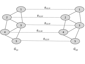
Thus, within each subgroup we assume a standard undirected graph with possible edges between all pairs of genes representing conditional dependencies as in a functional or regulatory pathway. Between different subgroups we only allow for relations between the same gene in different subgroups (different genes in different subgroups are assumed to be unconnected). This allows sharing information between subgroups and prognostic genes shared by different subgroups have a higher inclusion probability. To visualize this idea, Figure 1 shows an example network consisting of two subgroups, each with five predictors.
Graph selection prior on and
We infer the unknown graph and precision matrix using the structure learning approach for Gaussian graphical models by [22] (section 2.3). The precision matrix of subgroup corresponding to subgraph is denoted by . The corresponding prior is defined by
with fixed hyperparameters small, large and .
We assume the binary edge inclusion indicators within subgroup () as well as between subgroups and () to be independent Bernoulli a priori
with fixed prior probability of edge inclusion .
2.5 Posterior inference
The joint posterior distribution for the set of all parameters is proportional to the product of the joint likelihood and the prior distributions of the parameters in all subgroups
2.5.1 Markov chain Monte Carlo sampling
Markov Chain Monte Carlo (MCMC) simulations are required to obtain a posterior sample of the parameters. The different parameters are updated iteratively according to their conditional posterior distributions using a Gibbs sampler. A brief outline of the MCMC sampling scheme is given in the following. More details are provided in Supplementary Materials.
-
1.
For subgroup update with the block Gibbs sampler proposed by [22].
-
2.
Update all elements in iteratively with Gibbs sampler from the conditional distributions as well as , where () denotes all elements in except for ().
-
3.
Update all elements in iteratively with Gibbs sampler from the conditional distributions , where denotes all elements in except for .
-
4.
Update from the conditional distribution , , , using a random walk Metropolis-Hastings algorithm with adaptive jumping rule as proposed by [2]. includes all elements in except for .
-
5.
The conditional distribution for the update of can be well approximated by the gamma distribution
where is the number of events in interval for subgroup and denotes the vector without the -th element, , [20, chapter 3.2.2].
Starting with an arbitrary set of initial values for the parameters, the MCMC algorithm runs with a reasonably large number of iterations to obtain a representative sample from the posterior distribution. All subsequent results are based on single MCMC chains, each with 20 000 iterations in total and a burn-in period of 10 000 iterations. As starting values we choose an empty model with:
and for
for
for ,
for , .
We assessed convergence of each MCMC chain by looking at autocorrelations, trace plots and running mean plots of the regression coefficients. In addition, we ran several independent MCMC chains with different starting values to ensure that the chains and burn-in period were long enough to reach (approximate) convergence.
2.5.2 Posterior estimation and variable selection
We report the results of the Cox models in terms of marginal and conditional posterior means and standard deviations of the estimated regression coefficients, as well as posterior selection probabilities. After removal of the burn-in samples, the remaining MCMC samples serve as draws from the posterior distribution to calculate the empirical estimates. These estimates are then averaged across all training sets for each variable separately.
The strategy for variable selection follows [5]. First, the mean model size is computed as the average number of included variables across all MCMC iterations after the burn-in. Then the variables with the highest posterior selection probability are considered as the most important variables and selected in the final model.
2.5.3 Prediction
We use training data for model fitting and posterior estimation and test data to assess model performance. We evaluate the prediction performance of the Cox models by the integrated Brier score.
The expected Brier score can be interpreted as a mean square error of prediction. It measures the inaccuracy by comparing the estimated survival probability of a patient , , with the observed survival status
and the squared residuals are weighted using inverse probability of censoring weights
to adjust for the bias caused by the presence of censoring in the data. is the Kaplan-Meier estimator of the censoring times [23, 24].
The predictive performance of competing survival models can be compared by plotting the Brier score over time (prediction error curves). Alternatively, prediction error curves can be summarized in one value with the integrated Brier score as a measure of inaccuracy over a time interval rather than at single time points [25]
2.5.4 Median Probability Model and Bayesian Model Averaging
For the calculation of the prediction error, we account for the uncertainty in model selection by two different approaches: the Median Probability Model (MPM) [26] and an approximation to Bayesian Model Averaging (BMA) [27]. After removal of the burn-in samples, we compute the Brier score over the “best” selected models. According to the BMA approach we choose the top 100 models with the largest log-likelihood values to obtain the marginal posterior means of the regression coefficients, which in turn are required for the risk score. For the MPM approach we select all covariates with a mean posterior selection probability larger than 0.5. For these variables we calculate the marginal posterior means of the regression coefficients and the corresponding risk score.
3 Simulation study
In section 3.2 we compare the performance of our proposed model, referred to as CoxBVS-SL (for Cox model with Bayesian Variable Selection and Structure Learning, as an extension of the model by [5]), to a standard subgroup model and a combined model. The combined model pools data from all subgroups and treats them as one homogeneous cohort, whereas the subgroup model only uses information in the subgroup of interest and ignores the other subgroups. Both standard approaches follow the Bayesian Cox model proposed by [5] with stochastic search variable selection and independent Bernoulli priors for the variable inclusion indicators .
The priors for variable selection and structure learning are specified as follows. We set the hyperparameter of the Bernoulli distribution to , matching the prior probability of variable inclusion in the MRF prior of the CoxBVS-SL model. Based on a sensitivity analysis, we choose the hyperparameters of the MRF prior as and . When the graph contains no edges or then the prior variable inclusion probability is . This probability increases when is combined with a nonempty graph. The remaining hyperparameters for and are chosen as and , following the recommendations in [22] and [9].
We examine varying numbers of genomic covariates and sample sizes , with a focus on small sample sizes relative to the number of variables which is characteristic for gene expression data. We standardize the genomic covariates before model fitting and evaluation to have zero mean and unit variance. Parameters of the training data (mean and standard deviation of each variable) are used to scale the training and test data. For the standard subgroup model and the proposed model we standardize each subgroup separately, whereas for the combined model we pool training data of all subgroups.
For Bayesian inference, typically one training data set is used for posterior estimation and an independent test data set for model evaluation. However, results have shown some variation due to the data draw. Therefore, in the following, simulation of training and test data is repeated ten times for each simulation scenario.
In section 3.3 we use two different hyperparameters for the subgraphs , and in the MRF prior of the CoxBVS-SL model and compare the prediction performance with the Sub-struct model. In the latter is an empty graph and only information of is included in the MRF prior. We use the same training and test data as in section 3.2 but only consider simulation scenarios with .
3.1 Data simulation
Training and test data each consisting of samples and genomic covariates are simulated from the same distribution as described in the following. We consider two subgroups that differ only in their relationship between genomic covariates and survival endpoint (, ), and in the parameters for the simulation of survival data. We generate gene expression data from the same multivariate normal distribution with mean vector and covariance matrix . The corresponding precision matrix is defined such that the variance of each gene is 1 and partial correlations exist only between the first nine prognostic genes. Within the three blocks of prognostic genes determined by the same effect (gene 1 to 3, gene 4 to 6, and gene 7 to 9) we assume pairwise partial correlations of 0.5. All remaining genes are assumed to be uncorrelated.
We simulate survival data from a Weibull distribution according to [28], with scale and shape parameters estimated from two real gene expression cancer cohorts. Therefore, we compute survival probabilities at 3 and 5 years using the Kaplan-Meier estimator for both cohorts separately. The corresponding probabilities are 57% and 75% for 3-years survival, and 42% and 62% for 5-years survival, respectively. Individual event times for subgroup are simulated as
with true effects , . We randomly draw noninformative censoring times from a Weibull distribution with the same parameters as for the event times, resulting in approximately 50% censoring rates in both subgroups. The individual observed event indicators and times until an event or censoring are defined as and , .
We choose the true effects of the genomic covariates on survival outcome as stated in Table 1. Genes 1, 2, 3 and 7, 8, 9 are subgroup-specific, while genes 4, 5 and 6 have the same effect in both subgroups. All remaining genes represent noise and have no effect in both subgroups.
| Gene | ||||||||||||
|---|---|---|---|---|---|---|---|---|---|---|---|---|
| 1 | 2 | 3 | 4 | 5 | 6 | 7 | 8 | 9 | 10 | |||
| 1 | 1 | 1 | -1 | -1 | -1 | 0 | 0 | 0 | 0 | 0 | ||
| 0 | 0 | 0 | -1 | -1 | -1 | 1 | 1 | 1 | 0 | 0 | ||
3.2 Simulation results I
We consider three low-dimensional settings with genes and samples in each subgroup, as well as five high-dimensional settings with and sample sizes . We also tested and , but as expected, the results always lay between the results for and . For this reason, they are not shown here. We compare our proposed model (CoxBVS-SL) to the standard subgroup model (Subgroup) and the standard combined or pooled model (Pooled) regarding variable selection accuracy and prediction performance.
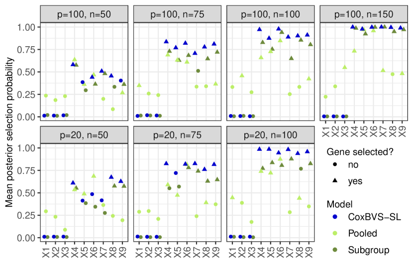
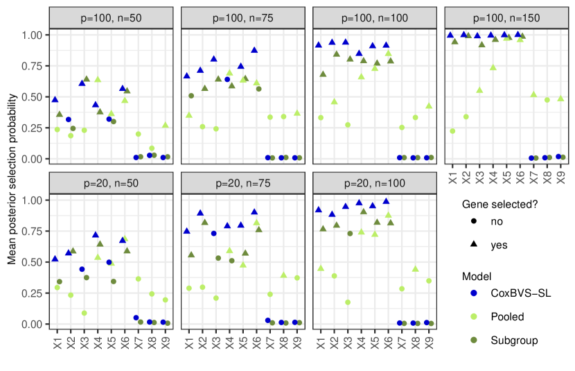
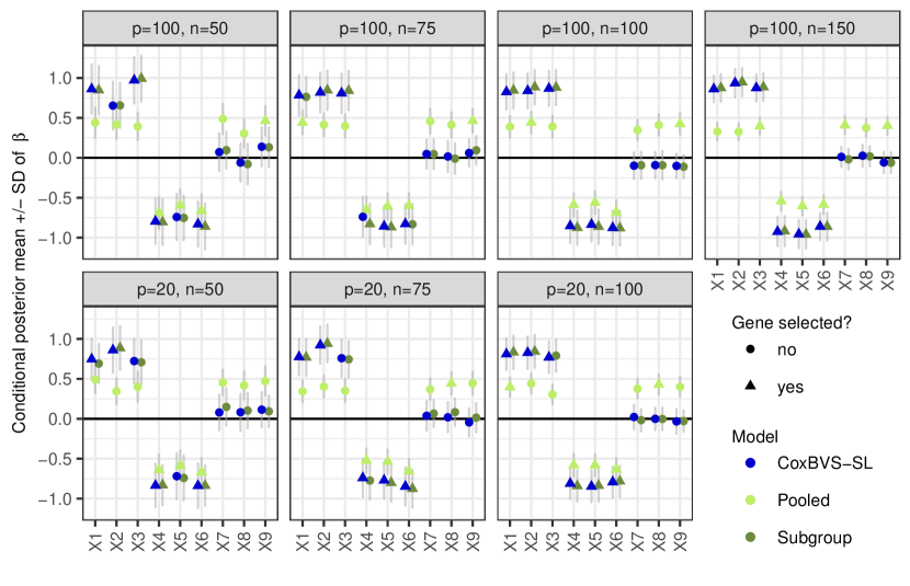
Posterior selection probabilities for each gene are computed based on all iterations after the burn-in and averaged across all training data sets. The resulting mean posterior selection probabilities of the first nine genes in subgroup 1 are depicted in Figure 2 (and in Supplementary Figure S1 for subgroup 2). Across all simulation scenarios, the CoxBVS-SL model has more power for the selection of prognostic genes compared to the two standard approaches, and at the same time, does not erroneously select noise genes (false positives) as the Pooled model. As expected, with larger , power and accuracy in variable selection increase for both, the CoxBVS-SL and the Subgroup model. The Pooled model only correctly identifies the joint effects of genes 4, 5 and 6 but fails to detect subgroup-specific effects.
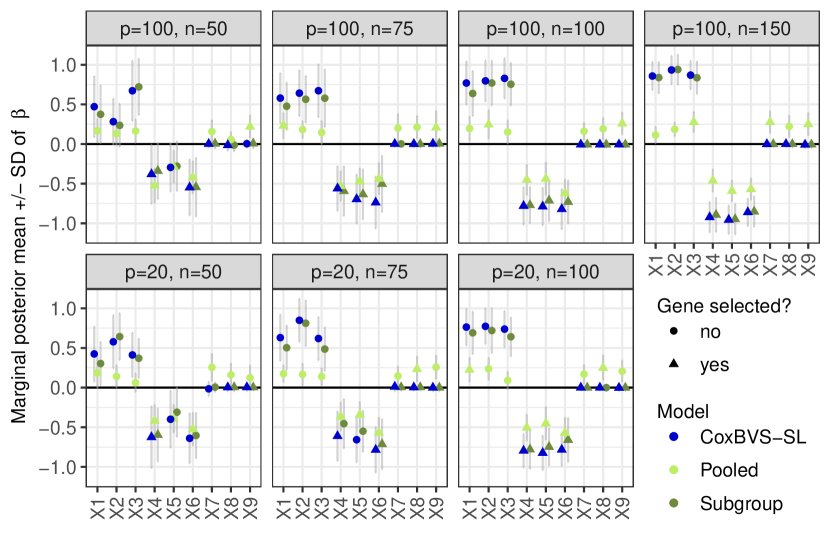
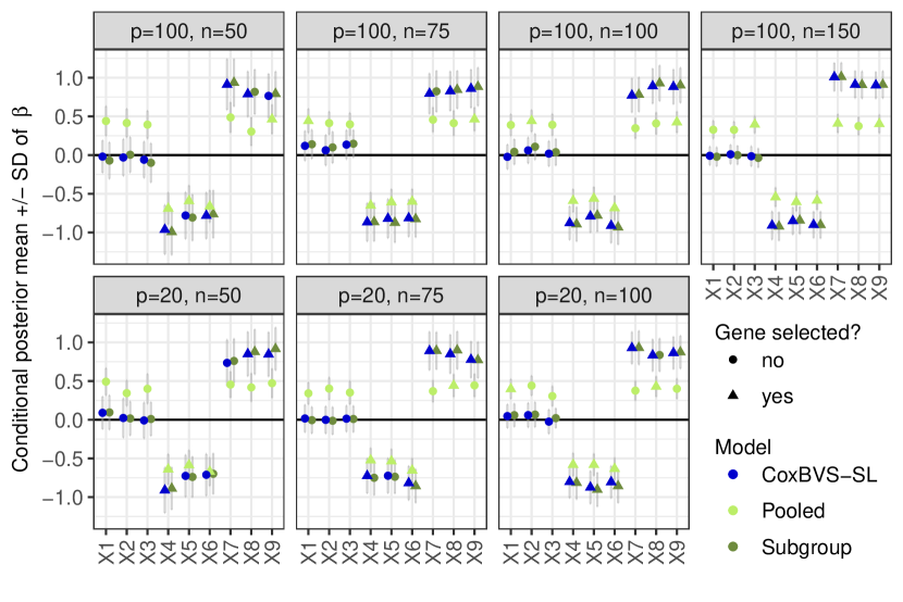
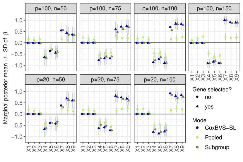
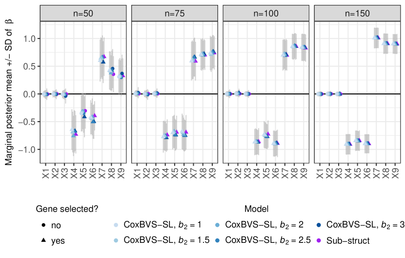
Posterior estimates of the regression coefficients of the first nine genes in subgroup 1 are shown in Figure 3 for conditional posterior means (conditional on ) and in Supplementary Figure S2 for marginal posterior means (independent of ), both along with standard deviations. The corresponding results for subgroup 2 are depicted in Supplementary Figures S3 and S4. For the conditional posterior means of the prognostic genes are less shrunk than the marginal posterior means. Results of the CoxBVS-SL model and the Subgroup model are very similar, whereas the Pooled model averages effects across subgroups leading to biased subgroup-specific effects and more false positives. Surprisingly, the joint effects of genes 4, 5 and 6 are also more precisely estimated (less shrunk) by CoxBVS-SL and Subgroup compared to Pooled.
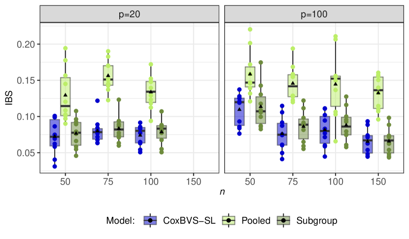
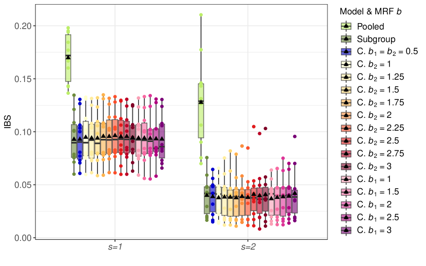
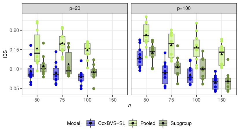
We assess prediction performance by the integrated Brier Score (IBS), computed based on the Median Probability Model (MPM, Figure 4 for subroup 1 and Supplementary Figure S6 for subgroup 2) and the Bayesian Model Averaging (BMA, Supplementary Figure S5 for subroup 1 and Supplementary Figure S7 for subgroup 2). The Pooled model has the worst prediction accuracy. In the case of MPM, CoxBVS-SL performs clearly better than Subgroup, for BMA both models are competitive.
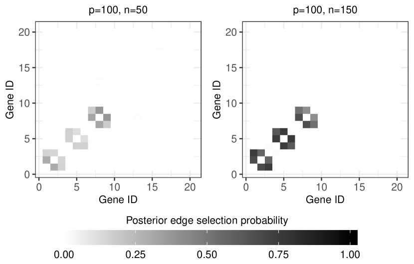
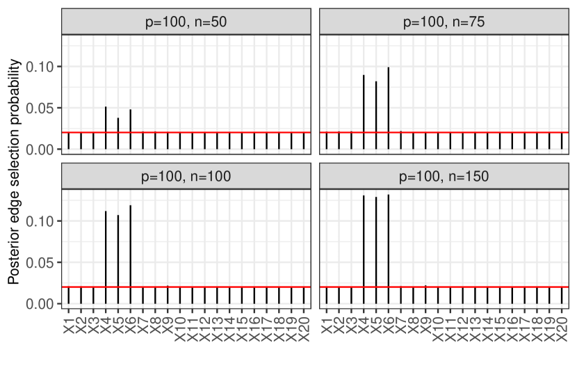
Inference of the graph showed relatively high accuracy for learning the conditional dependence structure among genes within subgroups and for detecting joint effects across different subgroups. The block correlation structure between the prognostic genes within each subgroup is correctly estimated by the precision matrix and the subgraph , in the CoxBVS-SL model (see Supplementary Figure S8). Inference of the subgraph linking both subgroups improves with increasing sample size. The corresponding marginal posterior edge inclusion probabilities of the prognostic genes with joint effects (genes 4, 5 and 6) are larger than for the remaining genes, which becomes more evident for increasing (see Supplementary Figure S9). Findings support the assumption that incorporating network information into variable selection may increase power to detect associations with the survival outcome and improve prediction accuracy.
3.3 Simulation results II
Next, we study the effect of two different hyperparameters in the MRF prior of the CoxBVS-SL model with respect to variable selection and prediction performance. The new hyperparameter corresponds to the subgraphs , within each subgroup and to the subgraph linking both subgroups. By choosing a larger value for , we give more weight in the MRF prior and thus, increase the prior variable inclusion probability for genes being simultaneously selected in both subgroups and having a link in .
We compare the results of CoxBVS-SL with varying to the results of the Sub-struct model where and only information of , is included in the MRF prior. In this comparison we investigate how much information is added by over . For the other hyperparameters we use the same values as in the previous section. We apply all models to the same training and test data sets as in section 3.2 but only consider simulation scenarios with and .
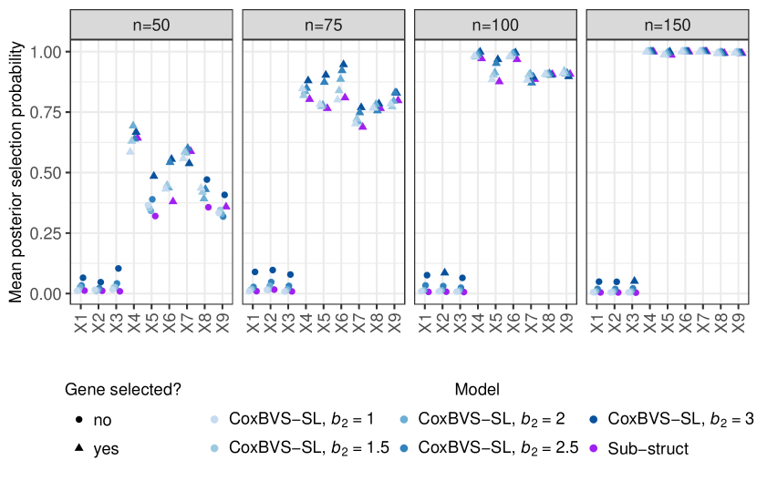
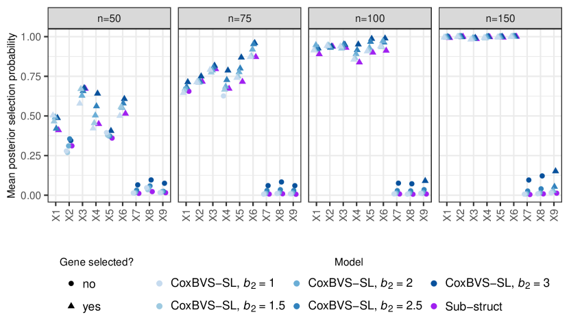
Figure 5 shows the mean posterior selection probabilities of the first nine genes in subgroup 1 (subgroup 2 is presented in Supplementary Figure S10). The results of Sub-struct are similar to CoxBVS-SL with . Increasing values of lead to larger posterior variable inclusion probabilities, however, not only for the prognostic genes (see genes 7, 8 and 9 in subgroup 1). This means more power for the correct identification of prognostic genes when , but on the other hand, a tendency towards more false positives.
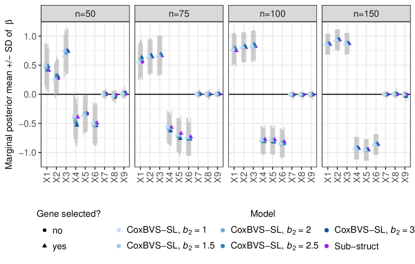
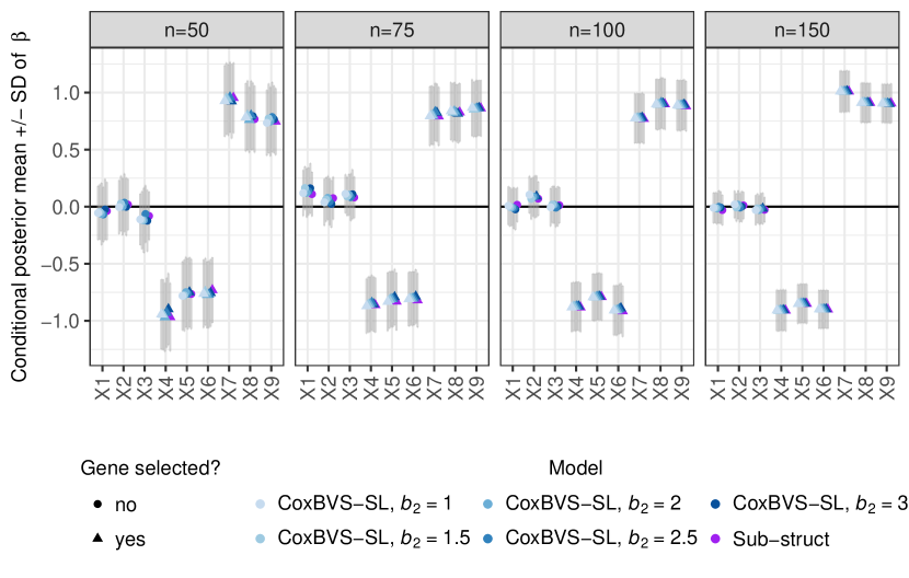
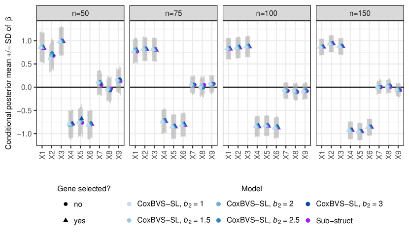
Posterior estimates of the regression coefficients are very similar for all models. Figure 6 shows the conditional posterior means (conditional on ) and Supplementary Figure S11 the marginal posterior means (independent of ) along with standard deviations of the first nine genes in subgroup 1. The corresponding results of subgroup 2 are depicted in Supplementary Figures S12 and S13.
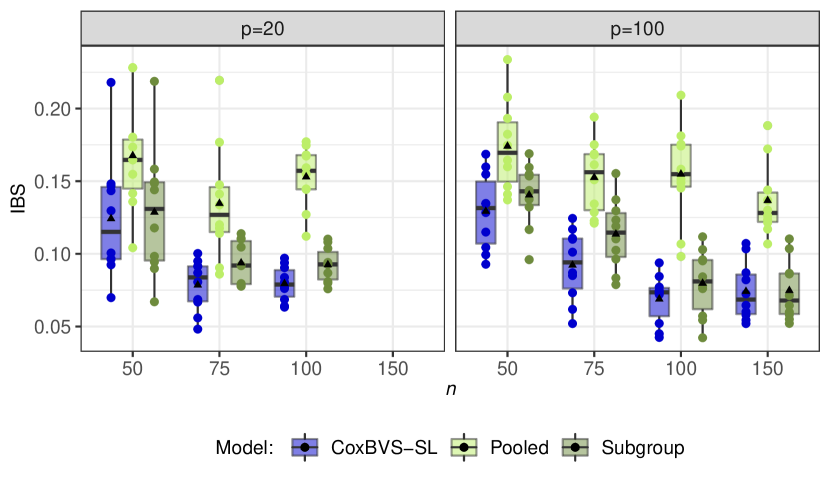
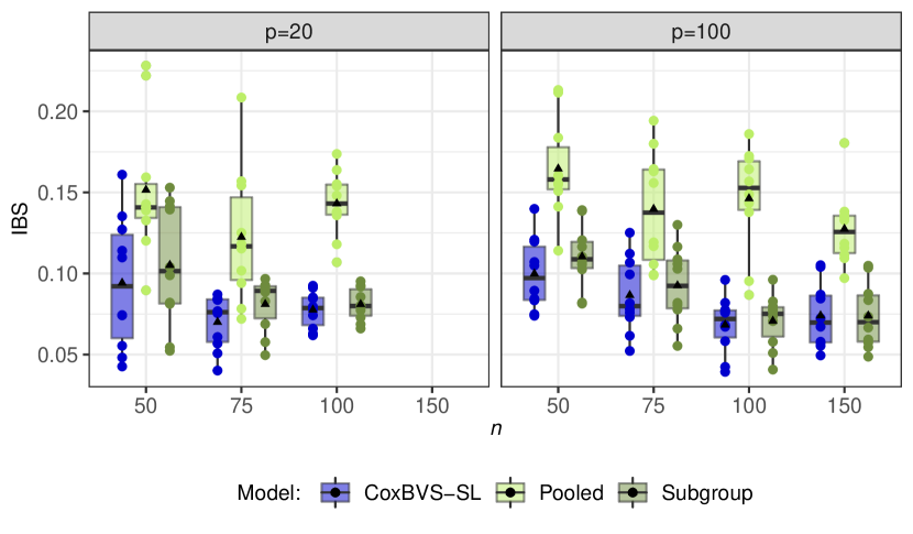
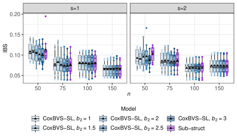
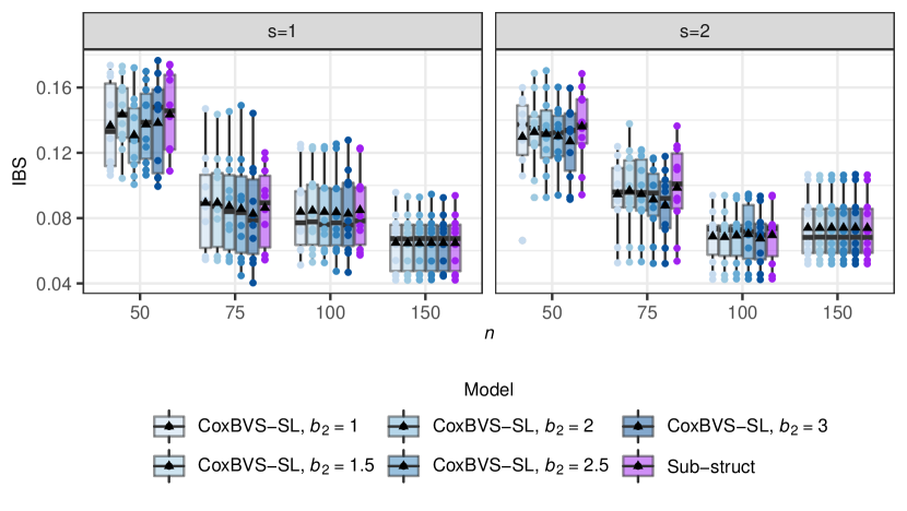
We assess prediction performance in terms of the integrated Brier Score (IBS), computed based on the Median Probability Model (Figure 7) and the Bayesian Model Averaging (Supplementary Figure S14). Larger values of tend to lead to a slightly better prediction performance of CoxBVS-SL compared to Sub-struct when . When the sample size is large, the prediction accuracy of all models is similarly good.
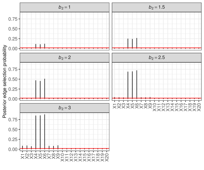
Supplementary Figure S15 compares the results of the subgraph for varying in CoxBVS-SL. For larger values of the marginal posterior edge inclusion probabilities of the prognostic genes with joint effects (genes 4, 5 and 6) increase, as expected, since they are given a higher weight in the prior. However, when we also notice a minor increase of the marginal posterior edge inclusion probabilities of the other six prognostic genes with subgroup-specific effects.
4 Case study based on Glioblastoma protein expression data
In this section we compare CoxBVS-SL with varying to both standard models, Pooled and Subgroup. We use the Glioblastoma protein expression data from [9], comprising 212 samples with survival data (159 events) and proteins. For reasons of computation time, we use only proteins and standardize the protein expression data as described in section 3. In contrast to the simulated gene expression data in the previous section, we have real correlations between all covariates and the data is not drawn from a multivariate normal distribution. We still simulate the relationship between proteins and survival outcome by choosing artificial effects and simulating the survival data from a Weibull distribution. We randomly divide the complete data set into two equally large subsets to obtain two subgroups.
For the survival endpoint we simulate the event times and censoring times , respectively, in subgroup from a Weibull distribution with scale and shape parameters estimated by the Kaplan-Meier estimator of the true event and censoring times, respectively, in the specific subgroup. The individual observed event indicators and survival times until an event or censoring are defined as and , resulting in approximately 42% censoring rates in both subgroups. The effects in subgroup and that we assume for the simulation of survival data are depicted in Table 2.
| Protein | ||
| Akt | 2 | 0 |
| Akt_pS473 | 2 | 0 |
| Akt_pT308 | 2 | 0 |
| EGFR | 0 | 2 |
| EGFR_pY1068 | 0 | 2 |
| EGFR_pY1173 | 0 | 2 |
| AMPK_alpha | -1.5 | 1.5 |
| Annexin.1 | 1.5 | -1.5 |
| GSK3.alpha.beta | -2 | -2 |
| GSK3.alpha.beta_pS21_S9 | -2 | -2 |
| GSK3_pS9 | -2 | -2 |
| X14.3.3_beta | 0 | 0 |
| X14.3.3_epsilon | 0 | 0 |
| X14.3.3_zeta | 0 | 0 |
| X4E.BP1 | 0 | 0 |
| X4E.BP1_pS65 | 0 | 0 |
| X4E.BP1_pT37T46 | 0 | 0 |
| X4E.BP1_pT70 | 0 | 0 |
| X53BP1 | 0 | 0 |
| A.Raf_pS299 | 0 | 0 |
We repeatedly randomly split the complete data into training (with proportion 0.8) and test sets, stratified by subgroup and event indicator. In total, we generate ten training data sets for model fitting and ten test data sets for evaluation of the prediction performance.
We choose the hyperparameters in accordance with the case study in [9] as follows. For the two standard models a prior probability of variable inclusion of 0.2 is assumed. In the CoxBVS-SL model we set the hyperparameters of the precision matrix and graph to and . The hyperparameters of the MRF prior are and as in section 3.3, we tried out two different values for : and , or and .
4.1 Results of the case study
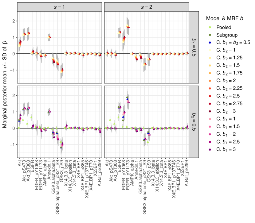
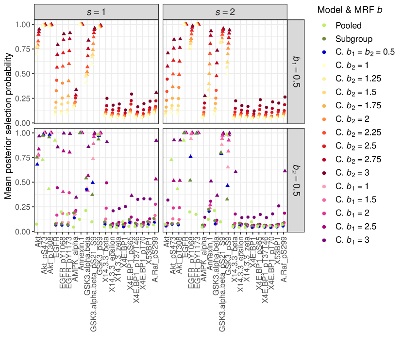
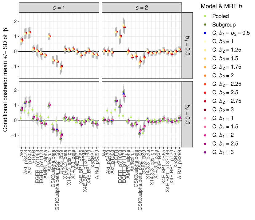
When either or increases the mean posterior selection probabilities of all proteins increase too (Figure 8). The Subgroup and CoxBVS-SL model with perform similarly. They correctly identify the subgroup-specific effects of the first six proteins and do not falsely select any noise proteins. Interestingly, the effects of proteins AMPK and Annexin (ID 7 and 8), going in opposite directions for both subgroups, as well as the joint effects of proteins GSK3 are not all identified. There are a few false negatives. The Pooled model, in contrast, shows a clear bias for the subgroup-specific and opposite effects. The effects are averaged across both subgroups, which also becomes evident when looking at the posterior estimates of the coefficients, for the conditional posterior means in Figure 9 and for the marginal posterior means in Supplementary Figure S16. The results of the Subgroup and CoxBVS-SL model are similar. In particular, the posterior means of the noise proteins are close to 0, also for large values of or .
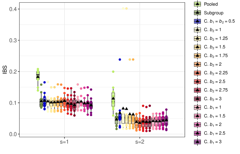
When we compare all models with regard to prediction accuracy in Figure 10 and Supplementary Figure S17, we again see competitive performance for the Subgroup and CoxBVS-SL model whereas Pooled is clearly worse. We can observe a tendency towards slightly improved prediction accuracy for increasing values of .
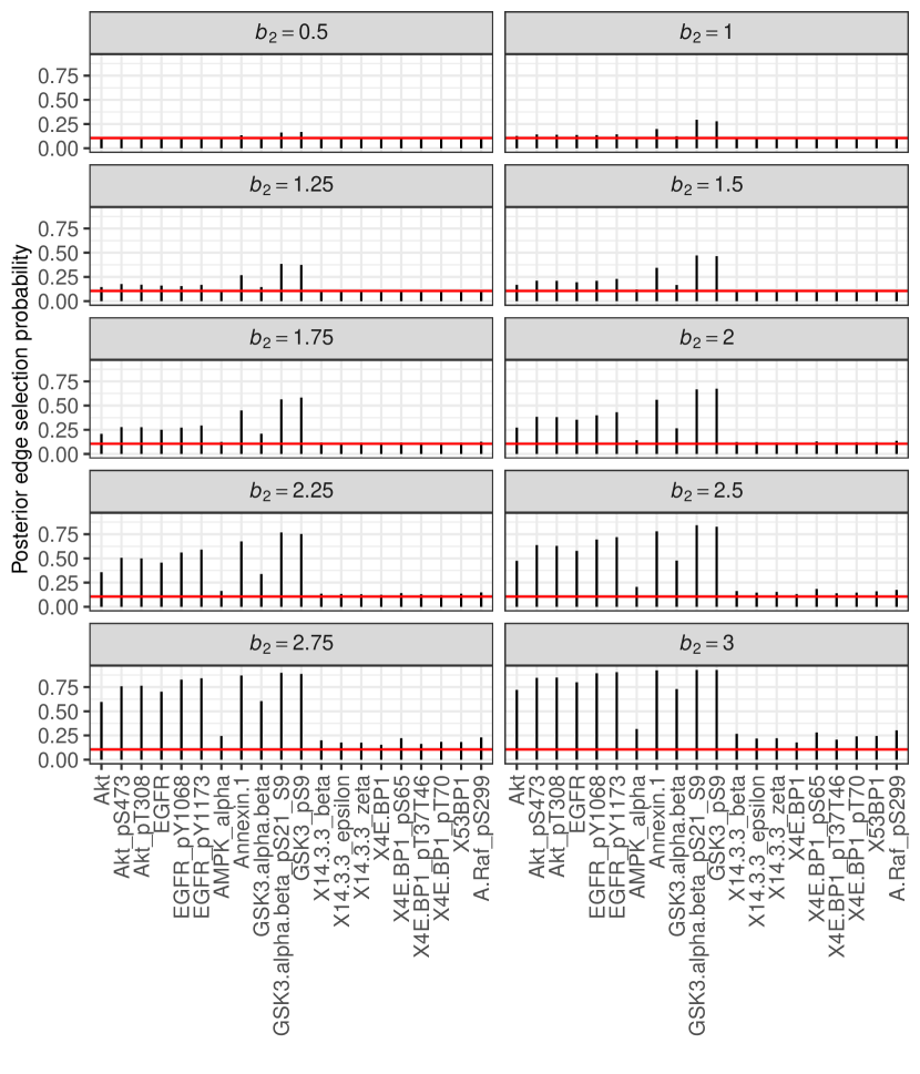
Finally, we assess the impact of increasing values of on the subgraph linking both subgroups. The corresponding marginal posterior edge selection probabilities are depicted in Supplementary Figure S18. When becomes larger first, the posterior edge selection probabilities of proteins 8, 10 and 11 with opposite or joint effects in both subgroups increase, followed by the first six proteins with subgroup-specific effects and protein 9 with joint effect. The posterior edge selection probabilities of the noise proteins in both subgroups remain at the prior mean and only start to increase slightly when . Proteins 7 and 9 have much smaller posterior edge selection probabilities than the other proteins with opposite or joint effects, which fits to previous findings.
When becomes larger, the marginal posterior edge selection probabilities in the subgraphs and show no visible changes. In they increase for some proteins however, to a much lesser extent than for larger .
5 Discussion
We consider the situation of different, possibly heterogeneous patients subgroups with survival endpoint and continuous molecular measurements such as gene expression data. When building a separate risk prediction model for each subgroup, it is important to consider heterogeneity but at the same time it can be reasonable to allow sharing information across subgroups to increase power, in particular when the sample sizes are small. For this situation we propose a hierarchical Cox model with stochastic search variable selection prior. To achieve higher power in variable selection and better prediction performance, we use an MRF prior instead of the standard Bernoulli prior for the latent variable selection indicators . The MRF prior leads to higher selection probabilities for genes that are related in an undirected graph. We use this graph to link genes across different subgroups and thereby borrow information between subgroups. Genes that are simultaneously prognostic in different subgroups have a higher probability of being selected into the respective subgroup Cox models. As a side aspect, the graph in the MRF prior also allows us to estimate a network between genes within each subgroup providing indications of functionally related genes and pathways. Here, genes that are conditionally dependent have a higher selection probability.
In the simulations and the case study we compared our proposed CoxBVS-SL model to the standard approach with independent Bernoulli prior for represented by the Subgroup and Pooled model. Simulations showed that the Pooled model performed worst in terms of variable selection and prediction accuracy. It averaged the effects across both subgroups and thus, led to biased estimates. CoxBVS-SL had more power in variable selection and slightly better prediction performance than Subgroup when the sample size was small. For both models were competitive.
In further simulations we studied the effect of increasing values of representing the weight that is given to the subgraph in the MRF prior of CoxBVS-SL and compared the results to the Sub-struct model where . When was small, CoxBVS-SL and Sub-struct performed very similarly. Thus, the subgraph linking both subgroups had only a small influence on the results compared to the conditional dependencies among covariates within each subgroup (subgraphs and ). For larger values of prediction performance slightly improved and power in variable selection increased but on the other hand, there was a tendency towards false positive variables.
In previous simulations we increased the weight for by choosing a larger value for the prior probability of edge inclusion for the corresponding edge inclusion indicators , . This led to larger posterior edge selection probabilities, however, for all genes and not only the ones with joint effects. The variable selection results did not change remarkably. We could observe a small increase in power for all genes which again implied a tendency towards false positives. We can conclude that a proper choice of (and ) in the MRF prior is crucial for the results of the graph and the Cox model.
We were able to demonstrate the superiority of our proposed model over the two standard approaches. This suggests that incorporating network information into variable selection can increase power to identify the prognostic covariates and improve prediction performance. However, in the case study the CoxBVS-SL and Subgroup model performed similarly well (Pooled was again clearly worse). The reason for this may be that the sample sizes in both subgroups were relatively large, in particular . Simulations had shown that CoxBVS-SL outperformed Subgroup only when and otherwise was competitive.
Due to computation time, we have included only up to 200 variables so far and the analysis of many thousands of genes is not (yet) feasible. An advantage of the CoxBVS-SL model is that it does not require prior knowledge of the graph among the covariates and between subgroups. It accounts for uncertainty over both variable and graph selection. In situations where pathway information is available and the graph structure is known, it is possible to incorporate this structural information in the MRF prior via a fixed graph.
Acknowledgements
This work was supported by Deutsche Forschungsgemeinschaft (DFG) within the Collaborative Research Center SFB 876 “Providing Information by Resource-Constrained Analysis”, project C4 (Katja Ickstadt) and project A3 (Jörg Rahnenführer), and by the Norwegian Research Council’s center for research-based innovation “BigInsight”, project number 237718 (Manuela Zucknick).
Supplementary Materials
Additional supporting information referenced in sections 2, 3 and 4 are available with this paper.
R source code for the models described in this paper and the preprocessed Glioblastoma data are available on GitHub:
https://github.com/KatrinMadjar/CoxBVS-SL.git.
References
- [1] T. Park and G. Casella (2008). The Bayesian Lasso. Journal of the American Statistical Association, 103(482): 681–686.
- [2] K. H. Lee, S. Chakraborty, and J. Sun (2011). Bayesian Variable Selection in Semiparametric Proportional Hazards Model for High Dimensional Survival Data. The International Journal of Biostatistics, 7(1): 1–32.
- [3] M. Zucknick, M. Saadati, and A. Benner (2015). Nonidentical twins: Comparison of frequentist and Bayesian lasso for Cox models. Biometrical Journal, 57(6): 959–981.
- [4] E. I. George and R. E. McCulloch (1993). Variable Selection via Gibbs Sampling. Journal of the American Statistical Association, 88(423): 881–889.
- [5] T. Treppmann, K. Ickstadt, and M. Zucknick (2017). Integration of Multiple Genomic Data Sources in a Bayesian Cox Model for Variable Selection and Prediction. Computational and Mathematical Methods in Medicine, vol. 2017, Article ID 7340565:19.
- [6] F. Li and N. R. Zhang (2010). Bayesian Variable Selection in Structured High-Dimensional Covariate Spaces With Applications in Genomics. Journal of the American Statistical Association, 105(491): 1202–1214.
- [7] F. C. Stingo and M. Vannucci (2011). Variable selection for discriminant analysis with Markov random field priors for the analysis of microarray data. Bioinformatics, 27(4): 495–501.
- [8] F. C. Stingo, Y. A. Chen, M. G. Tadesse, and M. Vannucci (2011). Incorporating biological information into linear models: A bayesian approach to the selection of pathways and genes. The Annals of Applied Statistics, 5(3): 1978–2002.
- [9] C. B. Peterson, F. C. Stingo, and M. Vannucci (2016). Joint Bayesian variable and graph selection for regression models with network-structured predictors. Statistics in Medicine, 35(7): 1017–1031.
- [10] S. Chakraborty and A. C. Lozano (2019). A graph Laplacian prior for Bayesian variable selection and grouping. Computational Statistics & Data Analysis, 136(C): 72–91.
- [11] P. Danaher, P. Wang, and D. M. Witten (2014). The joint graphical lasso for inverse covariance estimation across multiple classes. Journal of the Royal Statistical Society. Series B: Statistical Methodology, 76(2): 373–397.
- [12] T. Saegusa and A. Shojaie (2016). Joint estimation of precision matrices in heterogeneous populations. Electronic Journal of Statistics, 10(1): 1341–1392.
- [13] M. Yajima, D. Telesca, Y. Ji, and P. Muller (2012). Differential Patterns of Interaction and Gaussian Graphical Models. Collection of Biostatistics Research Archive, COBRA Preprint Series, 91.
- [14] R. Mitra, P. Müller, and Y. Ji (2016). Bayesian Graphical Models for Differential Pathways. Bayesian Analysis, 11(1): 99–124.
- [15] C. B. Peterson, F. C. Stingo, and M. Vannucci (2015). Bayesian Inference of Multiple Gaussian Graphical Models. Journal of the American Statistical Association, 110(509): 159–174.
- [16] V. Weyer and H. Binder (2015). A weighting approach for judging the effect of patient strata on high-dimensional risk prediction signatures. BMC Bioinformatics, 16:294.
- [17] J. Richter, K. Madjar, and J. Rahnenführer (2019). Model-based optimization of subgroup weights for survival analysis. Bioinformatics, 35(14): i484–i491.
- [18] K. Madjar and J. Rahnenführer (2020). Weighted cox regression for the prediction of heterogeneous patient subgroups. arXiv:2003.08965.
- [19] D. R. Cox (1972). Regression Models and Life-Tables. Journal of the Royal Statistical Society. Series B (Methodological), 34(2): 187–220.
- [20] J. G. Ibrahim, M.-H. Chen, and D. Sinha (2005). Bayesian survival analysis. Springer Series in Statistics. Springer, New York [u.a.], corr. 2nd print. edition.
- [21] M. Drton and M. H. Maathuis (2017). Structure learning in graphical modeling. Annual Review of Statistics and Its Application, 4(1): 365–393.
- [22] H. Wang (2015). Scaling It Up: Stochastic Search Structure Learning in Graphical Models. Bayesian Analysis, 10(2): 351–377.
- [23] M. Schumacher, H. Binder, and T. Gerds (2007). Assessment of survival prediction models based on microarray data. Bioinformatics, 23(14): 1768–1774.
- [24] H. Binder, C. Porzelius, and M. Schumacher (2011). An overview of techniques for linking high-dimensional molecular data to time-to-event endpoints by risk prediction models. Biometrical Journal, 53(2): 170–189.
- [25] E. Graf, C. Schmoor, W. Sauerbrei, and M. Schumacher (1999). Assessment and comparison of prognostic classification schemes for survival data. Statistics in Medicine, 18(17-18): 2529–2545.
- [26] M. M. Barbieri and J. O. Berger (2004). Optimal predictive model selection. The Annals of Statistics, 32(3): 870–897.
- [27] J. A. Hoeting, D. Madigan, A. E. Raftery, and C. T. Volinsky (1999). Bayesian model averaging: A tutorial. Statistical Science, 14(4): 382–401.
- [28] R. Bender, T. Augustin, and M. Blettner (2005). Generating survival times to simulate Cox proportional hazards models. Statistics in Medicine, 24(11): 1713–1723.
Supplementary Materials
Details of the MCMC algorithm
In the following, steps 1 to 4 of the MCMC sampling scheme in section 2.5.1 are explained in more detail.
Step 1: Update of
The block Gibbs sampler proposed by [22] is used to update for subgroups . The conditional distribution of is
Consider the following partitions
and analogously
where is a symmetric matrix with zeros on the diagonal.
For the block update of focus on the last column (and row) of :
with ,
.
The conditional distribution of the last column of is
Consider the following transformations
Then the conditional distribution is
,
.
Permuting any column in to be updated to the last one leads to a block Gibbs sampler for the update of .
Step 2: Update of
Update all elements in iteratively with Gibbs sampler from their conditional distributions. All elements are assumed independent Bernoulli a priori with and .
Update , , , (edges between the same gene in different subgroups) from the conditional distribution
where denotes all elements in except for . Accept with probability
where
This means, update as follows:
Update , , , (edges between different genes in the same subgroup) from the conditional distribution
where denotes all elements in except for . Accept with probability
where
Step 3: Update of
Update , , , with Gibbs sampler from the conditional distribution
where denotes all elements in except for . Accept with probability
where
Step 4: Update of
A random walk Metropolis-Hastings algorithm with adaptive jumping rule as proposed by [2] is used to update for and . The full conditional posterior distribution of is
where denotes the vector without the -th element. with .
In MCMC iteration update as follows:
-
(i)
Sample a proposal from a proposal distribution
-
(ii)
Calculate the ratio of ratios
-
(iii)
Accept the proposal if with .
The mean and variance of the proposal distribution can be approximated based on the first and second derivative of the log conditional posterior distribution with respect to .
Supplementary Figures
