ML
Machine Learning
DNN
Deep Neural Network
DP
Dynamic Programming
FBSDE
Forward-Backward Stochastic Differential Equation
FSDE
Forward Stochastic Differential Equation
BSDE
Backward Stochastic Differential Equation
LSTM
Long-Short Term Memory
FC
Fully Connected
DDP
Differential Dynamic Programming
HJB
Hamilton-Jacobi-Bellman
PDE
Partial Differential Equation
PI
Path Integral
NN
Neural Network
GPs
Gaussian Processes
SOC
Stochastic Optimal Control
RL
Reinforcement Learning
MPOC
Model Predictive Optimal Control
IL
Imitation Learning
RNN
Recurrent Neural Network
FNN
Feed-forward Neural Network
Single FNN
Single Feed-forward Neural Network
DL
Deep Learning
SGD
Stochastic Gradient Descent
SDE
Stochastic Differential Equation
2BSDE
second-order BSDE
CBF
Control Barrier Function
SCBF
Stochastic Control Barrier Function
SCLF
Stochastic Control Lyapunov Function
HDSCLF
High-Relative Degree Stochastic Control Lyapunov Function
QP
Quadratic Program
CBF
Control Barrier Function
PDIPM
Primal-Dual Interior Point Method

High-Relative Degree Stochastic Control Lyapunov and Barrier Functions

Meenakshi Sarkar1, Debasish Ghose2 and Evangelos A. Theodorou3 1Meenakshi Sarkar is with the Aerospace Engineering Department, Indian Institute of Science, Bangalore, India. This work was done during her stay as a visiting scholar at the Aerospace Engineering Department, Georgia Institute of Technology, USA meenakshisar@iisc.ac.in2Debasish Ghose is with the faculty of Aerospace Engineering Department, Indian Institute of Science, Bangalore, India. dghose@iisc.ac.in3Evangelos A. Theodorou is with the faculty of Aerospace Engineering Department, Georgia Institute of Technology, USA evangelos.theodorou@gatech.edu
Abstract

We introduce High-Relative Degree Stochastic Control Lyapunov functions and Barrier Functions as a means to ensure asymptotic stability of the system and incorporate state dependent high relative degree safety constraints on a non-linear stochastic systems. Our proposed formulation also provides a generalisation to the existing literature on control Lyapunov and barrier functions for stochastic systems. The control policies are evaluated using a constrained quadratic program that is based on control Lyapunov and barrier functions. Our proposed control design is validated via simulated experiments on a relative degree 2 system (2 dimensional car navigation) and relative degree 4 system (two-link pendulum with elastic actuator).

I Introduction

With the rapid advancement of autonomous systems in various sectors such as automobile, aviation, finance and medical, there has been a surge on research interest into safety verification of control systems. Safety plays a crucial role in various engineering application and thus researchers have investigated various methods such as barrier methods [1], reachable sets [2], and discrete approximations [3], to ensure safety certification of the system. Recently [4], [5] introduced Control Barrier Functions which aims at designing controllers with verifiable safety bounds.

While there has been a considerable amount of work on investigating barrier function methods based on the invariant set theorem [5] for designing safe controllers for deterministic systems, similar literature on stochastic systems is rather scarce. Only recently, [6] provided some sufficient conditions to satisfy safety constrains for stochastic systems. This work was limited in the sense that it was applicable only to scenarios where the constrained states are directly actuated. For systems where the observed states are not directly actuated via control gives rise to higher relative degree systems. For underactuated deterministic systems, [1] proposed exponential CBF and demonstrated its effectiveness on systems with relative degrees 6 and 4. Recent work by [7] tried to generalise the exponential barrier function approach and designed controller for an automatic cruise control problem. But currently there are no formation for a high relative degree control barrier function for stochastic systems. To the best of our knowledge, the present paper is the first attempt to generalise higher relative degree Stochastic Control Barrier Function (SCBF). Interestingly, in our formulation, the recent work on Stochastic Control Lyapunov Function (SCLF) by [6] turns out to be a special case where the relative degree of the system is one.

We further investigate the links between the formulation of SCBF and SCLF. There has been a considerable amount work [8], [9], [10], [11] done on investigating the stability of stochastic systems in the Lyapunov framework. Recently, [12] investigated the CLF-CBF formulation along with a Bayesian deep learning framework to design adaptive controllers for systems operating in uncertain environments. While the existing literature provide concrete foundation for Lyapunov function based stochastic controllers, they still do not provide a generalised framework that one can apply to systems with high relative degree or underactuated systems. While in the past the iLQG and dynamic programming framework [13] has been proven to be effective in case of stochastic systems, iLQG inherently assumes the system to be stabilizable which might not be the case for a underactuated system. Incidentally, there have been very few attempts in the past to address stability of stochastic systems with high relative degree.

In this paper we also provide a generalised Lyapunov function formulation for stochastic systems with high relative degree or high degree of underactuation. We also show how one can derive the existing formulation on SCLF [8], [11] as a special case where the relative degree is equal to one. For our analysis we assume complete system state information. The contributions of the paper are as follows:

  1. i)

    We propose a generalised high relative degree SCBF formulation and derive sufficient conditions for the system to satisfy safety constraints with probability 1.

  2. ii)

    We extend the high relative degree SCBF formulation to a generalised high relative degree SCLF formulation and derive sufficient conditions for asymptotic stability in the sense of probability.

  3. iii)

    We show that the previous formulations on stochastic CLF-CBF was a special case of our generalised formulation where the relative degree is 1.

  4. iv)

    We propose an approach to evaluate control policies using a stochastic CLF-CBF based quadratic programs. The stability and performance of the controller in probabilistic sense can be guaranteed via stochastic CLFs.

  5. v)

    We validate the proposed controller via simulated experiments on two different stochastic systems of high relative degree.

The rest of the paper is organised as follows: Section II provides the mathematical preliminaries and the problem formulation. Section III derives the generalised higher order SCBF and Section IV considers the higher order SCLF. We provide the controller formulation in Section V followed by simulations results on two high relative degree stochastic systems with relative degree 2 (2D car navigation) and 4 (2-link pendulum with elastic actuator) in Section VI. Finally we conclude the paper in Section VII.

II problem formulation and mathematical preliminaries

We consider the stochastic dynamics system as:

d𝐱(t)=(𝐟(𝐱(t))+𝐆(𝐱(t))𝐮(t))dt+𝚺(𝐱(t))d𝐰(t)d𝐱𝑡𝐟𝐱𝑡𝐆𝐱𝑡𝐮𝑡d𝑡𝚺𝐱𝑡d𝐰𝑡{\mathrm{d}}{\bf x}(t)=\big{(}{\bf f}({\bf x}(t))+{\bf G}({\bf x}(t)){\bf u}(t)\big{)}{\mathrm{d}}t+{\mbox{\boldmath$\Sigma$}}({\bf x}(t)){\mathrm{d}}{\bf w}(t) (1)

where, 𝐰(t)𝐰𝑡{\bf w}(t) is an nwsubscript𝑛𝑤n_{w} dimensional standard Brownian motion; 𝐱nx𝐱superscriptsubscript𝑛𝑥{\bf x}\in\mathbb{R}^{n_{x}}, and 𝐮(nu𝒰([0,T]){\bf u}\in\big{(}\mathbb{R}^{n_{u}}\cap{\cal{U}}([0,T]\big{)} denote the state and control vectors, respectively, where 𝒰([0,T])𝒰0𝑇{\cal{U}}([0,T]) represents the set of admissible controls for a fixed finite time horizon T[0,)𝑇0T\in[0,\infty) (i.e 0t<T<0𝑡𝑇0\leq t<T<\infty). The functions 𝐟:nxnx:𝐟superscriptsubscript𝑛𝑥superscriptsubscript𝑛𝑥{\bf f}:\mathbb{R}^{n_{x}}\rightarrow\mathbb{R}^{n_{x}}, 𝐆:nxnx×nu:𝐆superscriptsubscript𝑛𝑥superscriptsubscript𝑛𝑥subscript𝑛𝑢{\bf G}:\mathbb{R}^{n_{x}}\rightarrow\mathbb{R}^{n_{x}\times n_{u}} and 𝚺:nxnx×nw:𝚺superscriptsubscript𝑛𝑥superscriptsubscript𝑛𝑥subscript𝑛𝑤{\mbox{\boldmath$\Sigma$}}:\mathbb{R}^{n_{x}}\rightarrow\mathbb{R}^{n_{x}\times n_{w}} represent the uncontrolled system dynamics, the actuator dynamics, and the diffusion matrices, respectively.

The drift terms are assumed to be modelled as:

𝐚(𝐱,t)dt=(𝐟(𝐱(t))+𝐆(𝐱(t))𝐮(t))dt𝐚𝐱𝑡d𝑡𝐟𝐱𝑡𝐆𝐱𝑡𝐮𝑡d𝑡{\bf a}({\bf x},t){\mathrm{d}}t=\big{(}{\bf f}({\bf x}(t))+{\bf G}({\bf x}(t)){\bf u}(t)\big{)}{\mathrm{d}}t (2)

For the dynamical system defined by (1) safety is ensured if 𝐱(t)𝒞safe𝐱𝑡subscript𝒞𝑠𝑎𝑓𝑒{\bf x}(t)\in\mathcal{C}_{safe} for all t𝑡t, where the set 𝒞safesubscript𝒞𝑠𝑎𝑓𝑒\mathcal{C}_{safe} denotes the safe region of operation and is defined through a locally Lipschitz function h:nx:superscriptsubscript𝑛𝑥h:\mathbb{R}^{n_{x}}\rightarrow\mathbb{R} [4] as:

𝒞safesubscript𝒞𝑠𝑎𝑓𝑒\displaystyle\mathcal{C}_{safe} ={𝐱:h(𝐱)0}absentconditional-set𝐱𝐱0\displaystyle=\{{\bf x}:h({\bf x})\geq 0\}
δ𝒞safe𝛿subscript𝒞𝑠𝑎𝑓𝑒\displaystyle\delta\mathcal{C}_{safe} ={𝐱:h(𝐱)=0}.absentconditional-set𝐱𝐱0\displaystyle=\{{\bf x}:h({\bf x})=0\}.
Definition 1.

We define an SCBF B(𝐱):nx:𝐵𝐱superscriptsubscript𝑛𝑥B({\bf x}):\mathbb{R}^{n_{x}}\rightarrow\mathbb{R} which is locally Lipschitz and twice differentiable on int(𝒞safe)subscript𝒞𝑠𝑎𝑓𝑒(\mathcal{C}_{safe}), and satisfies the property that there exist class-K functions α1subscript𝛼1\alpha_{1}, α2subscript𝛼2\alpha_{2}, and α3subscript𝛼3\alpha_{3}, such that

1α1(h(𝐱))B(𝐱)1α2(h(𝐱)),𝐱𝒞safeformulae-sequence1subscript𝛼1𝐱𝐵𝐱1subscript𝛼2𝐱for-all𝐱subscript𝒞𝑠𝑎𝑓𝑒\frac{1}{\alpha_{1}(h({\bf x}))}\leq B({\bf x})\leq\frac{1}{\alpha_{2}(h({\bf x}))},\,\forall{\bf x}\in\mathcal{C}_{safe} (3)
B𝐱T(𝐟+𝐆𝐮)+12tr(2B𝐱2𝚺𝚺T)α3(h(𝐱)),tsuperscript𝐵𝐱T𝐟𝐆𝐮12trsuperscript2𝐵superscript𝐱2superscript𝚺𝚺Tsubscript𝛼3𝐱for-all𝑡\frac{\partial B}{\partial{\bf x}}^{\mathrm{T}}({\bf f}+{\bf G}{\bf u})+\frac{1}{2}\operatorname{\rm{tr}}\Big{(}\frac{\partial^{2}B}{\partial{\bf x}^{2}}{\mbox{\boldmath$\Sigma$}}{\mbox{\boldmath$\Sigma$}}^{\mathrm{T}}\Big{)}\leq\alpha_{3}(h({\bf x})),\,\forall t (4)
Theorem 1.

If there exists a SCBF of the form given in Definition 1 for a process given in Eqn. (1), then Pr(𝐱t𝒞safe)=1Prsubscript𝐱𝑡subscript𝒞𝑠𝑎𝑓𝑒1\text{Pr}({\bf x}_{t}\in\mathcal{C}_{safe})=1 for tfor-all𝑡\forall t given that x(t0)𝒞safe𝑥subscript𝑡0subscript𝒞𝑠𝑎𝑓𝑒x(t_{0})\in\mathcal{C}_{safe}. The detailed proof can be found in [6].

III High Relative Degree Stochastic Control Barrier Function

Definition 2.

Consider a Stochastic Dynamical System defined by Eq. (1) with safety set defined by 𝒞safesubscript𝒞𝑠𝑎𝑓𝑒\mathcal{C}_{safe}. We define a locally Lipschitz and twice-differentiable control barrier function B0(𝐱)::subscript𝐵0𝐱absentB_{0}({\bf x}): nxsuperscriptsubscript𝑛𝑥\mathbb{R}^{n_{x}}\rightarrow\mathbb{R} that satisfies Eqn. (3) and Eqn. (4) such that LgLfrb1B0(𝐱)u0subscript𝐿𝑔superscriptsubscript𝐿𝑓subscript𝑟𝑏1subscript𝐵0𝐱𝑢0\mathit{L}_{g}\mathit{L}_{f}^{r_{b}-1}B_{0}({\bf x})u\neq 0, and LgLfrb2B0(𝐱)u=LgLfrb3B0(𝐱)u==LgLfB0(𝐱)u=0subscript𝐿𝑔superscriptsubscript𝐿𝑓subscript𝑟𝑏2subscript𝐵0𝐱𝑢subscript𝐿𝑔superscriptsubscript𝐿𝑓subscript𝑟𝑏3subscript𝐵0𝐱𝑢subscript𝐿𝑔subscript𝐿𝑓subscript𝐵0𝐱𝑢0\mathit{L}_{g}\mathit{L}_{f}^{r_{b}-2}B_{0}({\bf x})u=\mathit{L}_{g}\mathit{L}_{f}^{r_{b}-3}B_{0}({\bf x})u=\cdots=\mathit{L}_{g}\mathit{L}_{f}B_{0}({\bf x})u=0. The function B0(𝐱)subscript𝐵0𝐱B_{0}({\bf x}) is said to be Stochastic Control Barrier Function with relative degree rbsubscript𝑟𝑏r_{b}. The function B(𝐱)𝐵𝐱B({\bf x}) in definition 1 is a special case where the relative degree of the control barrier function rb=1subscript𝑟𝑏1r_{b}=1.

Definition 3.

We define a sequence of safe sets as:

𝒞0=𝒞safesubscript𝒞0subscript𝒞𝑠𝑎𝑓𝑒\displaystyle\mathcal{C}_{0}=\mathcal{C}_{safe} ={𝐱:ψ0(𝐱)0}absentconditional-set𝐱subscript𝜓0𝐱0\displaystyle=\{{\bf x}:\psi_{0}({\bf x})\geq 0\}
δ𝒞0=δ𝒞safe𝛿subscript𝒞0𝛿subscript𝒞𝑠𝑎𝑓𝑒\displaystyle\delta\mathcal{C}_{0}=\delta\mathcal{C}_{safe} ={𝐱:ψ0(𝐱)=0}absentconditional-set𝐱subscript𝜓0𝐱0\displaystyle=\{{\bf x}:\psi_{0}({\bf x})=0\}
.𝒞1\displaystyle.\mathcal{C}_{1} ={𝐱:ψ1(𝐱)0}absentconditional-set𝐱subscript𝜓1𝐱0\displaystyle=\{{\bf x}:\psi_{1}({\bf x})\geq 0\}
δ𝒞1𝛿subscript𝒞1\displaystyle\delta\mathcal{C}_{1} ={𝐱:ψ1(𝐱)=0}absentconditional-set𝐱subscript𝜓1𝐱0\displaystyle=\{{\bf x}:\psi_{1}({\bf x})=0\}
\displaystyle\vdots
𝒞rbsubscript𝒞subscript𝑟𝑏\displaystyle\mathcal{C}_{r_{b}} ={𝐱:ψrb(𝐱)0}absentconditional-set𝐱subscript𝜓subscript𝑟𝑏𝐱0\displaystyle=\{{\bf x}:\psi_{r_{b}}({\bf x})\geq 0\}
δ𝒞rb=𝛿subscript𝒞subscript𝑟𝑏absent\displaystyle\delta\mathcal{C}_{r_{b}}= ={𝐱:ψrb(𝐱)=0}absentconditional-set𝐱subscript𝜓subscript𝑟𝑏𝐱0\displaystyle=\{{\bf x}:\psi_{r_{b}}({\bf x})=0\}

where ψisubscript𝜓𝑖\psi_{i} with i=0,1,,rb𝑖01subscript𝑟𝑏i=0,1,\cdots,r_{b} is defined as follows:

ψ0(𝐱)=h(𝐱)B0(𝐱)=γ0ψ0(𝐱)ψ1(𝐱)=α30(ψ0(𝐱))(B0T𝐱𝐚(𝐱)+12tr(2B0𝐱2𝚺𝚺T))B1(𝐱)=γ1ψ1(𝐱)ψ2(𝐱)=α31(ψ1(𝐱))(B1T𝐱𝐚(𝐱)+12tr(2B1𝐱2𝚺𝚺T))ψrb1(𝐱)=α3rb2(ψrb2(𝐱))Υrb2Brb1(𝐱)=γrb1ψrb1(𝐱)ψrb(𝐱)=α3rb1(ψrb1(𝐱))Υrb1subscript𝜓0𝐱𝐱subscript𝐵0𝐱subscript𝛾0subscript𝜓0𝐱subscript𝜓1𝐱superscriptsubscript𝛼30subscript𝜓0𝐱superscriptsubscript𝐵0𝑇𝐱𝐚𝐱12trsuperscript2subscript𝐵0superscript𝐱2superscript𝚺𝚺Tsubscript𝐵1𝐱subscript𝛾1subscript𝜓1𝐱subscript𝜓2𝐱superscriptsubscript𝛼31subscript𝜓1𝐱superscriptsubscript𝐵1𝑇𝐱𝐚𝐱12trsuperscript2subscript𝐵1superscript𝐱2superscript𝚺𝚺Tsubscript𝜓subscript𝑟𝑏1𝐱superscriptsubscript𝛼3subscript𝑟𝑏2subscript𝜓subscript𝑟𝑏2𝐱subscriptΥsubscript𝑟𝑏2subscript𝐵subscript𝑟𝑏1𝐱subscript𝛾subscript𝑟𝑏1subscript𝜓subscript𝑟𝑏1𝐱subscript𝜓subscript𝑟𝑏𝐱superscriptsubscript𝛼3subscript𝑟𝑏1subscript𝜓subscript𝑟𝑏1𝐱subscriptΥsubscript𝑟𝑏1\begin{split}\psi_{0}({\bf x})=&h({\bf x})\\ B_{0}({\bf x})=&\frac{\gamma_{0}}{\psi_{0}({\bf x})}\\ \psi_{1}({\bf x})=&\alpha_{3}^{0}(\psi_{0}({\bf x}))-\left(\frac{\partial B_{0}^{T}}{\partial{\bf x}}{\bf a}({\bf x})+\frac{1}{2}\operatorname{\rm{tr}}\Big{(}\frac{\partial^{2}B_{0}}{\partial{\bf x}^{2}}{\mbox{\boldmath$\Sigma$}}{\mbox{\boldmath$\Sigma$}}^{\mathrm{T}}\Big{)}\right)\\ B_{1}({\bf x})=&\frac{\gamma_{1}}{\psi_{1}({\bf x})}\\ \psi_{2}({\bf x})=&\alpha_{3}^{1}(\psi_{1}({\bf x}))-\left(\frac{\partial B_{1}^{T}}{\partial{\bf x}}{\bf a}({\bf x})+\frac{1}{2}\operatorname{\rm{tr}}\Big{(}\frac{\partial^{2}B_{1}}{\partial{\bf x}^{2}}{\mbox{\boldmath$\Sigma$}}{\mbox{\boldmath$\Sigma$}}^{\mathrm{T}}\Big{)}\right)\\ \vdots\\ \psi_{r_{b}-1}({\bf x})&=\alpha_{3}^{r_{b}-2}(\psi_{r_{b}-2}({\bf x}))-\Upsilon_{r_{b}-2}\\ B_{r_{b}-1}({\bf x})&=\frac{\gamma_{r_{b}-1}}{\psi_{r_{b}-1}({\bf x})}\\ \psi_{r_{b}}({\bf x})=&\alpha_{3}^{r_{b}-1}(\psi_{r_{b}-1}({\bf x}))-\Upsilon_{r_{b}-1}\\ \end{split}

where, Υj=(BjT𝐱𝐚(𝐱)+12tr(2Bj𝐱2𝚺𝚺T))subscriptΥ𝑗superscriptsubscript𝐵𝑗𝑇𝐱𝐚𝐱12trsuperscript2subscript𝐵𝑗superscript𝐱2superscript𝚺𝚺T\Upsilon_{j}=\left(\frac{\partial B_{j}^{T}}{\partial{\bf x}}{\bf a}({\bf x})+\frac{1}{2}\operatorname{\rm{tr}}\Big{(}\frac{\partial^{2}B_{j}}{\partial{\bf x}^{2}}{\mbox{\boldmath$\Sigma$}}{\mbox{\boldmath$\Sigma$}}^{\mathrm{T}}\Big{)}\right); γi+subscript𝛾𝑖superscript\gamma_{i}\in\mathbb{R}^{+} and α3isuperscriptsubscript𝛼3𝑖\alpha_{3}^{i}, with i{0,1,,rb1}𝑖01subscript𝑟𝑏1i\in\{0,1,\cdots,r_{b}-1\}, are class K function; Bi(𝐱)subscript𝐵𝑖𝐱B_{i}({\bf x}) are locally Lipschitz and twice differentiable on int(𝒞i)subscript𝒞𝑖(\mathcal{C}_{i}) and designed such that:

1α1i(ψi(𝐱))Bi(𝐱)1α2i(ψi(𝐱)),𝐱𝒞iformulae-sequence1superscriptsubscript𝛼1𝑖subscript𝜓𝑖𝐱subscript𝐵𝑖𝐱1superscriptsubscript𝛼2𝑖subscript𝜓𝑖𝐱for-all𝐱subscript𝒞𝑖\displaystyle\frac{1}{\alpha_{1}^{i}(\psi_{i}({\bf x}))}\leq B_{i}({\bf x})\leq\frac{1}{\alpha_{2}^{i}(\psi_{i}({\bf x}))},\,\forall{\bf x}\in\mathcal{C}_{i} (5)

Here, α1isuperscriptsubscript𝛼1𝑖\alpha_{1}^{i} and α2isuperscriptsubscript𝛼2𝑖\alpha_{2}^{i} for i=0,1,rb1𝑖01subscript𝑟𝑏1i=0,1,\cdots r_{b}-1, are all class K functions.

Theorem 2.

If x(t0)𝒞rb𝑥subscript𝑡0subscript𝒞subscript𝑟𝑏x(t_{0})\in\mathcal{C}_{r_{b}} and ψrb(𝐱)0subscript𝜓subscript𝑟𝑏𝐱0\psi_{r_{b}}({\bf x})\geq 0 then Pr(𝐱t𝒞safe)=1Prsubscript𝐱𝑡subscript𝒞𝑠𝑎𝑓𝑒1\text{Pr}({\bf x}_{t}\in\mathcal{C}_{safe})=1 for tfor-all𝑡\forall t where rbsubscript𝑟𝑏r_{b} denotes the relative degree of the control barrier function.

Proof.

The proof is done via induction. We onsider the case with rb=1subscript𝑟𝑏1r_{b}=1 we have

ψ1(𝐱)subscript𝜓1𝐱\displaystyle\psi_{1}({\bf x}) 0absent0\displaystyle\geq 0 (6)
(B0T𝐱𝐚(𝐱)+12tr(2B0𝐱2𝚺𝚺T))absentsuperscriptsubscript𝐵0𝑇𝐱𝐚𝐱12trsuperscript2subscript𝐵0superscript𝐱2superscript𝚺𝚺T\displaystyle\implies\big{(}\frac{\partial B_{0}^{T}}{\partial{\bf x}}{\bf a}({\bf x})+\frac{1}{2}\operatorname{\rm{tr}}\Big{(}\frac{\partial^{2}B_{0}}{\partial{\bf x}^{2}}{\mbox{\boldmath$\Sigma$}}{\mbox{\boldmath$\Sigma$}}^{\mathrm{T}}\Big{)}\big{)} α30(ψ0(𝐱))absentsuperscriptsubscript𝛼30subscript𝜓0𝐱\displaystyle\leq\alpha_{3}^{0}(\psi_{0}({\bf x})) (7)
(B0T𝐱𝐚(𝐱)+12tr(2B0𝐱2𝚺𝚺T))absentsuperscriptsubscript𝐵0𝑇𝐱𝐚𝐱12trsuperscript2subscript𝐵0superscript𝐱2superscript𝚺𝚺T\displaystyle\implies\big{(}\frac{\partial B_{0}^{T}}{\partial{\bf x}}{\bf a}({\bf x})+\frac{1}{2}\operatorname{\rm{tr}}\Big{(}\frac{\partial^{2}B_{0}}{\partial{\bf x}^{2}}{\mbox{\boldmath$\Sigma$}}{\mbox{\boldmath$\Sigma$}}^{\mathrm{T}}\Big{)}\big{)} α30(h0(𝐱))absentsuperscriptsubscript𝛼30subscript0𝐱\displaystyle\leq\alpha_{3}^{0}(h_{0}({\bf x})) (8)

From Eq (8) along with the Eq.(5) we can say

Pr(𝐱t𝒞0)=1Prsubscript𝐱𝑡subscript𝒞01\displaystyle\text{Pr}({\bf x}_{t}\in\mathcal{C}_{0})=1
Pr(𝐱t𝒞safe)=1absentPrsubscript𝐱𝑡subscript𝒞𝑠𝑎𝑓𝑒1\displaystyle\implies\text{Pr}({\bf x}_{t}\in\mathcal{C}_{safe})=1

This directly follows from the proof given in [6].

Now assume that the relative degree of the CBF is j𝑗j. Now, from Theorem 1. we have

ψj(𝐱)subscript𝜓𝑗𝐱\displaystyle\psi_{j}({\bf x}) 0absent0\displaystyle\geq 0 (9)
(Bj1T𝐱𝐚(𝐱)+12tr(2Bj1𝐱2𝚺𝚺T))absentsuperscriptsubscript𝐵𝑗1𝑇𝐱𝐚𝐱12trsuperscript2subscript𝐵𝑗1superscript𝐱2superscript𝚺𝚺T\displaystyle\implies\big{(}\frac{\partial B_{j-1}^{T}}{\partial{\bf x}}{\bf a}({\bf x})+\frac{1}{2}\operatorname{\rm{tr}}\Big{(}\frac{\partial^{2}B_{j-1}}{\partial{\bf x}^{2}}{\mbox{\boldmath$\Sigma$}}{\mbox{\boldmath$\Sigma$}}^{\mathrm{T}}\Big{)}\big{)} α30(ψj1(𝐱))absentsuperscriptsubscript𝛼30subscript𝜓𝑗1𝐱\displaystyle\leq\alpha_{3}^{0}(\psi_{j-1}({\bf x})) (10)

Following the proof given for stochastic CBF in [6] we can derive that given Eq. 10 and Eq 5,

Pr(𝐱t𝒞j1)=1 for tPrsubscript𝐱𝑡subscript𝒞𝑗11 for for-all𝑡\displaystyle\text{Pr}({\bf x}_{t}\in\mathcal{C}_{j-1})=1\text{ for }\forall t

Now, given 𝐱𝒞j1𝐱subscript𝒞𝑗1{\bf x}\in\mathcal{C}_{j-1} for tfor-all𝑡\forall t we can say that

ψj1(𝐱)subscript𝜓𝑗1𝐱\displaystyle\psi_{j-1}({\bf x}) 0absent0\displaystyle\geq 0 (11)
(Bj2T𝐱𝐚(𝐱)+12tr(2Bj2𝐱2𝚺𝚺T))absentsuperscriptsubscript𝐵𝑗2𝑇𝐱𝐚𝐱12trsuperscript2subscript𝐵𝑗2superscript𝐱2superscript𝚺𝚺T\displaystyle\implies\big{(}\frac{\partial B_{j-2}^{T}}{\partial{\bf x}}{\bf a}({\bf x})+\frac{1}{2}\operatorname{\rm{tr}}\Big{(}\frac{\partial^{2}B_{j-2}}{\partial{\bf x}^{2}}{\mbox{\boldmath$\Sigma$}}{\mbox{\boldmath$\Sigma$}}^{\mathrm{T}}\Big{)}\big{)} α30(ψj2(𝐱))absentsuperscriptsubscript𝛼30subscript𝜓𝑗2𝐱\displaystyle\leq\alpha_{3}^{0}(\psi_{j-2}({\bf x})) (12)

With Eq. 12 and Eq. 5 we can again prove that:

Pr(𝐱t𝒞j2)=1 for tPrsubscript𝐱𝑡subscript𝒞𝑗21 for for-all𝑡\displaystyle\text{Pr}({\bf x}_{t}\in\mathcal{C}_{j-2})=1\text{ for }\forall t

Thus, with the property of induction and Eq 8 and Eq 5 we can iteratively prove that

Pr(𝐱t𝒞j2)Prsubscript𝐱𝑡subscript𝒞𝑗2\displaystyle\text{Pr}({\bf x}_{t}\in\mathcal{C}_{j-2}) =1 for tabsent1 for for-all𝑡\displaystyle=1\text{ for }\forall t
Pr(𝐱t𝒞j3)absentPrsubscript𝐱𝑡subscript𝒞𝑗3\displaystyle\implies\text{Pr}({\bf x}_{t}\in\mathcal{C}_{j-3}) =1 for tabsent1 for for-all𝑡\displaystyle=1\text{ for }\forall t
\displaystyle\vdots
Pr(𝐱t𝒞1)absentPrsubscript𝐱𝑡subscript𝒞1\displaystyle\implies\text{Pr}({\bf x}_{t}\in\mathcal{C}_{1}) =1 for tabsent1 for for-all𝑡\displaystyle=1\text{ for }\forall t
Pr(𝐱t𝒞0)absentPrsubscript𝐱𝑡subscript𝒞0\displaystyle\implies\text{Pr}({\bf x}_{t}\in\mathcal{C}_{0}) =1 for tabsent1 for for-all𝑡\displaystyle=1\text{ for }\forall t
Pr(𝐱t𝒞safe)absentPrsubscript𝐱𝑡subscript𝒞𝑠𝑎𝑓𝑒\displaystyle\implies\text{Pr}({\bf x}_{t}\in\mathcal{C}_{safe}) =1 for tabsent1 for for-all𝑡\displaystyle=1\text{ for }\forall t

Corollary 1.

𝒞rb𝒞rb1𝒞1𝒞0subscript𝒞subscript𝑟𝑏subscript𝒞subscript𝑟𝑏1subscript𝒞1subscript𝒞0\mathcal{C}_{r_{b}}\subseteq\mathcal{C}_{r_{b}-1}\subseteq\cdots\subseteq\mathcal{C}_{1}\subseteq\mathcal{C}_{0}

Proof.

This can be easily derived from Theorem 2. ∎

Remark 1.

It can be noted from Theorem 2 that

BiT𝐱𝐚(𝐱)=BiT𝐱𝐟(𝐱) for i=0,1,,rb2formulae-sequencesuperscriptsubscript𝐵𝑖𝑇𝐱𝐚𝐱superscriptsubscript𝐵𝑖𝑇𝐱𝐟𝐱 for 𝑖01subscript𝑟𝑏2\displaystyle\frac{\partial B_{i}^{T}}{\partial{\bf x}}{\bf a}({\bf x})=\frac{\partial B_{i}^{T}}{\partial{\bf x}}{\bf f}({\bf x})\text{ for }i=0,1,\cdots,r_{b}-2

and

Brb1T𝐱𝐚(𝐱)=Brb1T𝐱(𝐟(𝐱)+𝐆𝐮)superscriptsubscript𝐵subscript𝑟𝑏1𝑇𝐱𝐚𝐱superscriptsubscript𝐵subscript𝑟𝑏1𝑇𝐱𝐟𝐱𝐆𝐮\displaystyle\frac{\partial B_{r_{b}-1}^{T}}{\partial{\bf x}}{\bf a}({\bf x})=\frac{\partial B_{r_{b}-1}^{T}}{\partial{\bf x}}({\bf f}({\bf x})+{\bf G}{\bf u})

IV High Relative Degree Stochastic Control Lyapunov Function

Definition 4.

A solution x(t)0𝑥𝑡0x(t)\equiv 0 of equation 1 is said to be stable in probability for t0𝑡0t\geq 0 if for any s0𝑠0s\geq 0 and ϵ>0italic-ϵ0\epsilon>0

limη0𝐏{supt>s|xs,η(t)|>ϵ}=0𝜂0lim𝐏𝑡𝑠supsuperscript𝑥𝑠𝜂𝑡italic-ϵ0\underset{\eta\rightarrow 0}{\mathrm{lim}}\mathbf{P}\left\{\underset{t>s}{\mathrm{sup}}\left|x^{s,\eta}(t)\right|>\epsilon\right\}=0
Theorem 3.

Let U𝑈U be a domain containing the line x=0𝑥0x=0 and there exist a smooth positive definite function V(𝐱)20(U)𝑉𝐱superscriptsubscript20𝑈V({\bf x})\in\mathbb{C}_{2}^{0}(U) s.t V(𝐱):nx+:𝑉𝐱superscriptsubscript𝑛𝑥subscriptV({\bf x}):\mathbb{R}^{n_{x}}\rightarrow\mathbb{R}_{+} that satisfies

LfV+LGVu+12tr{2V𝐱2ΣΣT}0subscript𝐿𝑓𝑉subscript𝐿𝐺𝑉𝑢12trsuperscript2𝑉superscript𝐱2ΣsuperscriptΣ𝑇0\mathit{L}_{f}V+\mathit{L}_{G}Vu+\frac{1}{2}\textrm{tr}\{\frac{\partial^{2}V}{\partial{\bf x}^{2}}\Sigma\Sigma^{T}\}\leq 0

The function V(𝐱)𝑉𝐱V({\bf x}) is known as the Stochastic Control Lyapunov Function SCLF. Detailed proof can be found in [11]

Definition 5.

A solution x(t)0𝑥𝑡0x(t)\equiv 0 of equation 1 is said to be asymptotically stable if it is stable in probability and moreover

limη0𝐏{limtxs,η(t)=0}=1𝜂0lim𝐏𝑡limsuperscript𝑥𝑠𝜂𝑡01\underset{\eta\rightarrow 0}{\mathrm{lim}}\mathbf{P}\left\{\underset{t\rightarrow\infty}{\mathrm{lim}}x^{s,\eta}(t)=0\right\}=1
Theorem 4.

The system 1 is globally asymptotically stabilizable in probability if there exist a SCLF that satisfies

LfV+LGVu+12tr{2V𝐱2ΣΣT}<0subscript𝐿𝑓𝑉subscript𝐿𝐺𝑉𝑢12trsuperscript2𝑉superscript𝐱2ΣsuperscriptΣ𝑇0\mathit{L}_{f}V+\mathit{L}_{G}Vu+\frac{1}{2}\textrm{tr}\{\frac{\partial^{2}V}{\partial{\bf x}^{2}}\Sigma\Sigma^{T}\}<0

Detailed proof can be found in [11] and [8]

Definition 6.

Let there exist a smooth function V0(𝐱)subscript𝑉0𝐱V_{0}({\bf x}) that satisfies the conditions given in theorem 4 such that, LGLfrl1V0(𝐱)u0subscript𝐿𝐺superscriptsubscript𝐿𝑓subscript𝑟𝑙1subscript𝑉0𝐱𝑢0\mathit{L}_{G}\mathit{L}_{f}^{r_{l}-1}V_{0}({\bf x})u\neq 0 and LGLfrb2V0(𝐱)u=LGLfrl3V(𝐱)u==LGLfV0(𝐱)u=0subscript𝐿𝐺superscriptsubscript𝐿𝑓subscript𝑟𝑏2subscript𝑉0𝐱𝑢subscript𝐿𝐺superscriptsubscript𝐿𝑓subscript𝑟𝑙3𝑉𝐱𝑢subscript𝐿𝐺subscript𝐿𝑓subscript𝑉0𝐱𝑢0\mathit{L}_{G}\mathit{L}_{f}^{r_{b}-2}V_{0}({\bf x})u=\mathit{L}_{G}\mathit{L}_{f}^{r_{l}-3}V({\bf x})u=\cdots=\mathit{L}_{G}\mathit{L}_{f}V_{0}({\bf x})u=0. The function V(𝐱)𝑉𝐱V({\bf x}) is said to be Stochastic Control Lyapunov Function with relative degree rlsubscript𝑟𝑙r_{l}.
The function V(𝐱)𝑉𝐱V({\bf x}) defined in theorem 4 is a special case where the relative degree of the SCLF, rl=1subscript𝑟𝑙1r_{l}=1

Definition 7.

Define a sequence of Lyapunov sets as:

1=stablesubscript1subscript𝑠𝑡𝑎𝑏𝑙𝑒\displaystyle\mathcal{L}_{1}=\mathcal{L}_{stable} ={𝐱:χ1(𝐱)0}absentconditional-set𝐱subscript𝜒1𝐱0\displaystyle=\{{\bf x}:\chi_{1}({\bf x})\geq 0\}
δ1=δstable𝛿subscript1𝛿subscript𝑠𝑡𝑎𝑏𝑙𝑒\displaystyle\delta\mathcal{L}_{1}=\delta\mathcal{L}_{stable} ={𝐱:χ1(𝐱)=0}absentconditional-set𝐱subscript𝜒1𝐱0\displaystyle=\{{\bf x}:\chi_{1}({\bf x})=0\}
2subscript2\displaystyle\mathcal{L}_{2} ={𝐱:χ2(𝐱)0}absentconditional-set𝐱subscript𝜒2𝐱0\displaystyle=\{{\bf x}:\chi_{2}({\bf x})\geq 0\}
δ2𝛿subscript2\displaystyle\delta\mathcal{L}_{2} ={𝐱:χ2(𝐱)=0}absentconditional-set𝐱subscript𝜒2𝐱0\displaystyle=\{{\bf x}:\chi_{2}({\bf x})=0\}
\displaystyle\vdots
rlsubscriptsubscript𝑟𝑙\displaystyle\mathcal{L}_{r_{l}} ={𝐱:χrl(𝐱)0}absentconditional-set𝐱subscript𝜒subscript𝑟𝑙𝐱0\displaystyle=\{{\bf x}:\chi_{r_{l}}({\bf x})\geq 0\}
δrl=𝛿subscriptsubscript𝑟𝑙absent\displaystyle\delta\mathcal{L}_{r_{l}}= ={𝐱:χrl(𝐱)=0}absentconditional-set𝐱subscript𝜒subscript𝑟𝑙𝐱0\displaystyle=\{{\bf x}:\chi_{r_{l}}({\bf x})=0\}

where, we define χisubscript𝜒𝑖\chi_{i} with i=0,1,,rl𝑖01subscript𝑟𝑙i=0,1,\cdots,r_{l} as follows:

g(𝐱)=𝑔𝐱absent\displaystyle g({\bf x})= d(LfV0+LGV0u+12tr{2V0𝐱2ΣΣT})𝑑subscript𝐿𝑓subscript𝑉0subscript𝐿𝐺subscript𝑉0𝑢12trsuperscript2subscript𝑉0superscript𝐱2ΣsuperscriptΣ𝑇\displaystyle d-\big{(}\mathit{L}_{f}V_{0}+\mathit{L}_{G}V_{0}u+\frac{1}{2}\textrm{tr}\{\frac{\partial^{2}V_{0}}{\partial{\bf x}^{2}}\Sigma\Sigma^{T}\}\big{)}
χ1(𝐱)=subscript𝜒1𝐱absent\displaystyle\chi_{1}({\bf x})= g(𝐱)𝑔𝐱\displaystyle g({\bf x})
V1(𝐱)=subscript𝑉1𝐱absent\displaystyle V_{1}({\bf x})= υ1χ1(𝐱)subscript𝜐1subscript𝜒1𝐱\displaystyle\frac{\upsilon_{1}}{\chi_{1}({\bf x})}
χ2(𝐱)=subscript𝜒2𝐱absent\displaystyle\chi_{2}({\bf x})= β31(χ1(𝐱))(V1T𝐱𝐚(𝐱)+12tr(2V1𝐱2𝚺𝚺T))superscriptsubscript𝛽31subscript𝜒1𝐱superscriptsubscript𝑉1𝑇𝐱𝐚𝐱12trsuperscript2subscript𝑉1superscript𝐱2superscript𝚺𝚺T\displaystyle\beta_{3}^{1}(\chi_{1}({\bf x}))-\left(\frac{\partial V_{1}^{T}}{\partial{\bf x}}{\bf a}({\bf x})+\frac{1}{2}\operatorname{\rm{tr}}\Big{(}\frac{\partial^{2}V_{1}}{\partial{\bf x}^{2}}{\mbox{\boldmath$\Sigma$}}{\mbox{\boldmath$\Sigma$}}^{\mathrm{T}}\Big{)}\right)
V2(𝐱)=subscript𝑉2𝐱absent\displaystyle V_{2}({\bf x})= υ2χ2(𝐱)subscript𝜐2subscript𝜒2𝐱\displaystyle\frac{\upsilon_{2}}{\chi_{2}({\bf x})}
χ3(𝐱)=subscript𝜒3𝐱absent\displaystyle\chi_{3}({\bf x})= β32(χ2(𝐱))(V2T𝐱𝐚(𝐱)+12tr(2V2𝐱2𝚺𝚺T))superscriptsubscript𝛽32subscript𝜒2𝐱superscriptsubscript𝑉2𝑇𝐱𝐚𝐱12trsuperscript2subscript𝑉2superscript𝐱2superscript𝚺𝚺T\displaystyle\beta_{3}^{2}(\chi_{2}({\bf x}))-\left(\frac{\partial V_{2}^{T}}{\partial{\bf x}}{\bf a}({\bf x})+\frac{1}{2}\operatorname{\rm{tr}}\Big{(}\frac{\partial^{2}V_{2}}{\partial{\bf x}^{2}}{\mbox{\boldmath$\Sigma$}}{\mbox{\boldmath$\Sigma$}}^{\mathrm{T}}\Big{)}\right)
\displaystyle\vdots
χrl1(𝐱)subscript𝜒subscript𝑟𝑙1𝐱\displaystyle\chi_{r_{l}-1}({\bf x}) =β3rl2(χrl2(𝐱))Zrl2absentsuperscriptsubscript𝛽3subscript𝑟𝑙2subscript𝜒subscript𝑟𝑙2𝐱subscript𝑍subscript𝑟𝑙2\displaystyle=\beta_{3}^{r_{l}-2}(\chi_{r_{l}-2}({\bf x}))-\mathit{Z}_{r_{l}-2}
Vrl1(𝐱)subscript𝑉subscript𝑟𝑙1𝐱\displaystyle V_{r_{l}-1}({\bf x}) =υrb1χrb1(𝐱)absentsubscript𝜐subscript𝑟𝑏1subscript𝜒subscript𝑟𝑏1𝐱\displaystyle=\frac{\upsilon_{r_{b}-1}}{\chi_{r_{b}-1}({\bf x})}
χrl(𝐱)=subscript𝜒subscript𝑟𝑙𝐱absent\displaystyle\chi_{r_{l}}({\bf x})= β3rl1(χrb1(𝐱))Zrl1superscriptsubscript𝛽3subscript𝑟𝑙1subscript𝜒subscript𝑟𝑏1𝐱subscript𝑍subscript𝑟𝑙1\displaystyle\beta_{3}^{r_{l}-1}(\chi_{r_{b}-1}({\bf x}))-\mathit{Z}_{r_{l}-1}

where, Zj=(VjT𝐱𝐚(𝐱)+12tr(2Vj𝐱2𝚺𝚺T))subscript𝑍𝑗superscriptsubscript𝑉𝑗𝑇𝐱𝐚𝐱12trsuperscript2subscript𝑉𝑗superscript𝐱2superscript𝚺𝚺T\mathit{Z}_{j}=\left(\frac{\partial V_{j}^{T}}{\partial{\bf x}}{\bf a}({\bf x})+\frac{1}{2}\operatorname{\rm{tr}}\Big{(}\frac{\partial^{2}V_{j}}{\partial{\bf x}^{2}}{\mbox{\boldmath$\Sigma$}}{\mbox{\boldmath$\Sigma$}}^{\mathrm{T}}\Big{)}\right) and d𝑑d\in\mathbb{R} is the relaxation variable. υi+subscript𝜐𝑖superscript\upsilon_{i}\in\mathbb{R}^{+} and β3isuperscriptsubscript𝛽3𝑖\beta_{3}^{i}s are class K functions where i{1,,rl1}𝑖1subscript𝑟𝑙1i\in\{1,\cdots,r_{l}-1\} . Vi(𝐱)subscript𝑉𝑖𝐱V_{i}({\bf x}) are are locally Lipschitz, twice differentiable on int(i)subscript𝑖(\mathcal{L}_{i}) and designed such that:

1β1i(χi(𝐱))Vi(𝐱)1β2i(χi(𝐱)),𝐱iformulae-sequence1superscriptsubscript𝛽1𝑖subscript𝜒𝑖𝐱subscript𝑉𝑖𝐱1superscriptsubscript𝛽2𝑖subscript𝜒𝑖𝐱for-all𝐱subscript𝑖\displaystyle\frac{1}{\beta_{1}^{i}(\chi_{i}({\bf x}))}\leq V_{i}({\bf x})\leq\frac{1}{\beta_{2}^{i}(\chi_{i}({\bf x}))},\,\forall{\bf x}\in\mathcal{L}_{i} (13)

Here β1isuperscriptsubscript𝛽1𝑖\beta_{1}^{i} and β2isuperscriptsubscript𝛽2𝑖\beta_{2}^{i} for i=1,rb1𝑖1subscript𝑟𝑏1i=1,\cdots r_{b}-1 are all class K functions.

Theorem 5.

If x(t0)rl𝑥subscript𝑡0subscriptsubscript𝑟𝑙x(t_{0})\in\mathcal{L}_{r_{l}} and χrl(𝐱)0subscript𝜒subscript𝑟𝑙𝐱0\chi_{r_{l}}({\bf x})\geq 0, then the system governed with equation 1 is globally asymptotically stabilizable in probability.

Proof.

From theorem 2 we can show that given, χrl(𝐱)0subscript𝜒subscript𝑟𝑙𝐱0\chi_{r_{l}}({\bf x})\geq 0,

Pr(𝐱tstable)=1 for t,Prsubscript𝐱𝑡subscript𝑠𝑡𝑎𝑏𝑙𝑒1 for for-all𝑡\displaystyle\text{Pr}({\bf x}_{t}\in\mathcal{L}_{stable})=1\text{ for }\forall t, (14)

Using theorem 4 we can easily show that system will be globally asymptotically stabilizable in probability. ∎

Corollary 2.

rlrl121subscriptsubscript𝑟𝑙subscriptsubscript𝑟𝑙1subscript2subscript1\mathcal{L}_{r_{l}}\subseteq\mathcal{L}_{r_{l}-1}\subseteq\cdots\subseteq\mathcal{L}_{2}\subseteq\mathcal{L}_{1}

Proof.

This can be easily derived from Theorem 5. ∎

Remark 2.

It can be noted from Theorem 5 that

ViT𝐱𝐚(𝐱)=ViT𝐱𝐟(𝐱) for i=0,1,,rb2formulae-sequencesuperscriptsubscript𝑉𝑖𝑇𝐱𝐚𝐱superscriptsubscript𝑉𝑖𝑇𝐱𝐟𝐱 for 𝑖01subscript𝑟𝑏2\displaystyle\frac{\partial V_{i}^{T}}{\partial{\bf x}}{\bf a}({\bf x})=\frac{\partial V_{i}^{T}}{\partial{\bf x}}{\bf f}({\bf x})\text{ for }i=0,1,\cdots,r_{b}-2

and

Vrl1T𝐱𝐚(𝐱)=Vrl1T𝐱(𝐟(𝐱)+𝐆𝐮)superscriptsubscript𝑉subscript𝑟𝑙1𝑇𝐱𝐚𝐱superscriptsubscript𝑉subscript𝑟𝑙1𝑇𝐱𝐟𝐱𝐆𝐮\displaystyle\frac{\partial V_{r_{l}-1}^{T}}{\partial{\bf x}}{\bf a}({\bf x})=\frac{\partial V_{r_{l}-1}^{T}}{\partial{\bf x}}({\bf f}({\bf x})+{\bf G}{\bf u})

V Control Policies from SCLF-SCBF based Quadratic Programs

In this section we discuss how the control policies are formulated in the form of a Quadratic Program (QP) based on High-Relative Degree Stochastic Control Lyapunov Function (HDSCLF) and CBF. The details of HDSCLF-CBF based QP are as follows:
 

HDSCLF-CBF-QP:

𝐮=superscript𝐮absent\displaystyle{\bf u}^{*}= argmin𝐮,d𝐮𝑑argmin\displaystyle\underset{{\bf u},d}{\mathrm{argmin}}\text{ } 𝐮TQ𝐮+pd2superscript𝐮𝑇𝑄𝐮𝑝superscript𝑑2\displaystyle{\bf u}^{T}Q{\bf u}+pd^{2} (15)
s.t. χrl(𝐱)0subscript𝜒subscript𝑟𝑙𝐱0\displaystyle\chi_{r_{l}}({\bf x})\geq 0 (SCLF)
ψrb(𝐱)0subscript𝜓subscript𝑟𝑏𝐱0\displaystyle\psi_{r_{b}}({\bf x})\geq 0 (SCBF)
𝐮upper𝐮𝐮lowersubscript𝐮𝑢𝑝𝑝𝑒𝑟𝐮subscript𝐮𝑙𝑜𝑤𝑒𝑟\displaystyle{\bf u}_{upper}\geq{\bf u}\geq{\bf u}_{lower} (Constraint)

  Equation 15 denotes the cost of QP subjected to the SCLF and SCBF conditions and the higher and lower limits of the control effort.

VI Simulation Results

In order to validate our proposed method we consider two tasks: 2D car navigation in the presence of multiple obstacle (non-linear system with relative degree 2) and swinging a 2-link pendulum with elastic actuator (relative degree 4 system with 2 degree underactuation). We assume the noise only enters through the control channels similar to [14] and [15]. The details of the simulated experiments and results are as follows:

VI-A Two-dimensional Car navigation (Relative Degree 2)

We validate our proposed method on a relatively complex and nonlinear scenarios of a two-dimensional car navigation. We consider a simple 2D circle following a simplified car dynamics as given in [16] for a time horizon T=8𝑇8T=8s :

x˙=vsin(θ),˙𝑥𝑣𝑠𝑖𝑛𝜃\displaystyle\dot{x}=vsin(\theta), y˙=vcos(θ)˙𝑦𝑣𝑐𝑜𝑠𝜃\displaystyle\dot{y}=vcos(\theta)
θ˙=vuθ,˙𝜃𝑣superscript𝑢𝜃\displaystyle\dot{\theta}=vu^{\theta}, v˙=uv˙𝑣superscript𝑢𝑣\displaystyle\dot{v}=u^{v}

where 𝐱=[x,y,θ,v]𝐱𝑥𝑦𝜃𝑣{\bf x}=[x,y,\theta,v] denotes the state of the car which includes 2D position, orientation and forward velocity. Control variables uθsuperscript𝑢𝜃u^{\theta} and uvsuperscript𝑢𝑣u^{v} changes the steering angle and forward velocity respectively. Here we want to find control policies to navigate the car from the initial x-y position of [0,0]00[0,0] with orientation of [0,0]00[0,0] to the final goal position [xdesired,ydesired]=[4,4]subscript𝑥𝑑𝑒𝑠𝑖𝑟𝑒𝑑subscript𝑦𝑑𝑒𝑠𝑖𝑟𝑒𝑑44[x_{desired},y_{desired}]=[4,4] in the presence of single and multiple obstacles. The 2D constraints on the positional states from the obstacle avoidance problem leads to a relative degree 2 control barrier function as the positional states are not directly actuated. The controller also tries to reach the target position while avoiding the obstacles which leads to a relative degree 2 control Lyapunov function formulation. The control Lyapunov function was defined as :

V0(𝐱)=12((xxdesired)2+(yydesired)2)subscript𝑉0𝐱12superscript𝑥subscript𝑥𝑑𝑒𝑠𝑖𝑟𝑒𝑑2superscript𝑦subscript𝑦𝑑𝑒𝑠𝑖𝑟𝑒𝑑2V_{0}({\bf x})=\frac{1}{2}\big{(}(x-x_{desired})^{2}+(y-y_{desired})^{2}\big{)}

The barrier function and the safe sets for each obstacle i𝑖i are defined as follows:

ψ0i(𝐱)superscriptsubscript𝜓0𝑖𝐱\displaystyle\psi_{0}^{i}({\bf x}) =hi(𝐱)=((xixci)2+(yixci)2(ri)2)absentsuperscript𝑖𝐱superscriptsuperscript𝑥𝑖subscriptsuperscript𝑥𝑖𝑐2superscriptsuperscript𝑦𝑖subscriptsuperscript𝑥𝑖𝑐2superscriptsuperscript𝑟𝑖2\displaystyle=h^{i}({\bf x})=\big{(}(x^{i}-x^{i}_{c})^{2}+(y^{i}-x^{i}_{c})^{2}-(r^{i})^{2}\big{)}
𝒞safeisuperscriptsubscript𝒞𝑠𝑎𝑓𝑒𝑖\displaystyle\mathcal{C}_{safe}^{i} ={𝐱:ψ0i(𝐱)0}absentconditional-set𝐱superscriptsubscript𝜓0𝑖𝐱0\displaystyle=\{{\bf x}:\psi_{0}^{i}({\bf x})\geq 0\}
B0i(𝐱)superscriptsubscript𝐵0𝑖𝐱\displaystyle B_{0}^{i}({\bf x}) =γ0iψ0i(𝐱)absentsuperscriptsubscript𝛾0𝑖superscriptsubscript𝜓0𝑖𝐱\displaystyle=\frac{\gamma_{0}^{i}}{\psi_{0}^{i}({\bf x})}

and

𝒞safe=i=1no𝒞safeisubscript𝒞𝑠𝑎𝑓𝑒superscriptsubscript𝑖1subscript𝑛𝑜superscriptsubscript𝒞𝑠𝑎𝑓𝑒𝑖\mathcal{C}_{safe}=\bigcup_{i=1}^{n_{o}}\mathcal{C}_{safe}^{i}

Where (xci,yci)subscriptsuperscript𝑥𝑖𝑐subscriptsuperscript𝑦𝑖𝑐(x^{i}_{c},y^{i}_{c}) and risuperscript𝑟𝑖r^{i} denote the 2D position of the centre and radius of the ith obstacle respectively. nosubscript𝑛𝑜n_{o} represents the no of obstacle present.
Refer to caption
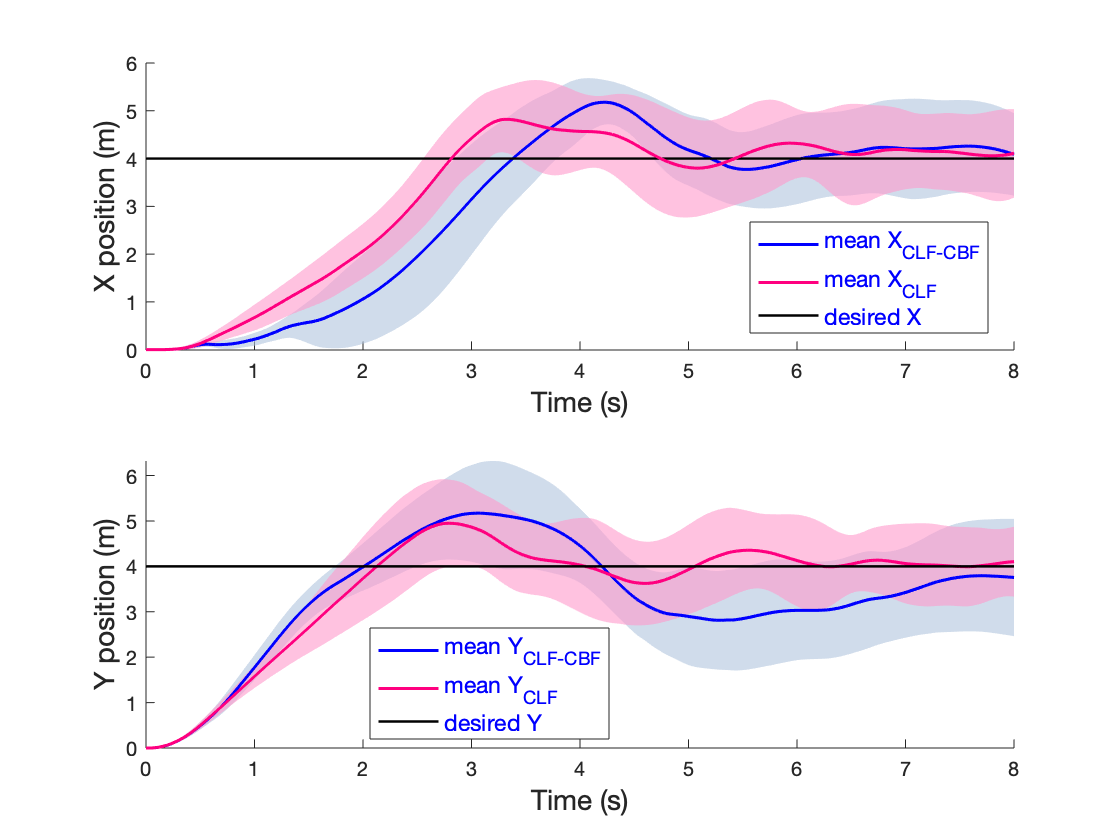
Figure 1: Multiple obstacle avoidance Task: The mean and the sigma distribution of the x𝑥x and y𝑦y state trajectories for the CLF-CBF controller and the CLF controller are plotted here in sheds of blue and green respectively.

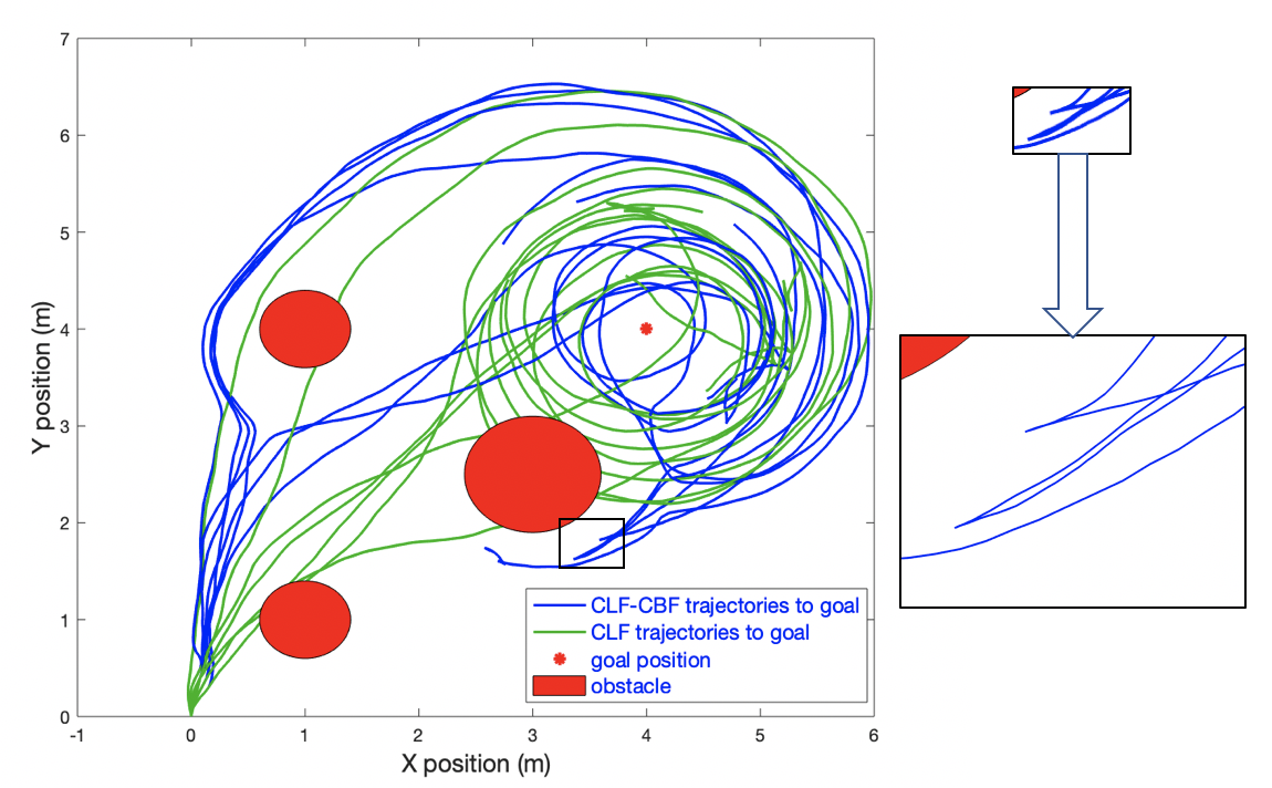
For our simulations of single obstacle the centre and radius was taken as (3,2.5)32.5(3,2.5)m and 0.6m respectively. For the multiple obstacle case we took 3 obstacles placed at (1,1)11(1,1)m, (1,4)14(1,4)m and (3,2.5)32.5(3,2.5)m with radius of 0.4m,0.4m and 0.6m respectively. The diagonal elements of the Q𝑄Q matrix are chosen as [1000,10]100010[1000,10] and p=1000𝑝1000p=1000. We simulated 20 sample trajectories for the experiments and the multiple obstacle avoidance task are shown in figure 1 and figure 2. Interestingly from the enlarged portion of figure 2 we can see for the HDSCLF-CBF controller the trajectories take a U-turn after encountering the obstacle and moves towards the goal point. The circular trajectories around the goal point in figure 2 is expected due to the asymptotic nature of the stability in the sense of probability from theorem 5.
Refer to caption
Figure 2: Multiple obstacle avoidance task: 7 test trajectories out of the 20 sample trajectories are shown here. The green ones generated with the CLF controller show no regard for the obstacles where as the blue ones from the CLF-CBF controller successfully avoids all the 3 obstacles in all cases. The selected enlarged portion shows how the blue trajectories takes a U-turn when they encountered the obstacle shown in red.

VI-B 2-Link Pendulum with Elastic Actuators (Relative Deg. 4)

Here we consider a two link pendulum with elastic actuator described in [1]. The two-link pendulum is a system with 4 degrees of freedom and two degrees of underactuation. The commanded torques τ1subscript𝜏1\tau_{1} and τ2subscript𝜏2\tau_{2} of the two motors in the two elastic actuators will generate torque at the two joints indirectly through the following motor dynamics:

Jmθ¨1m=k(θ1θ1m)+τ1subscript𝐽𝑚superscriptsubscript¨𝜃1𝑚𝑘subscript𝜃1superscriptsubscript𝜃1𝑚subscript𝜏1\displaystyle J_{m}\ddot{\theta}_{1}^{m}=k(\theta_{1}-\theta_{1}^{m})+\tau_{1}
Jmθ¨2m=k(θ2θ2m)+τ2subscript𝐽𝑚superscriptsubscript¨𝜃2𝑚𝑘subscript𝜃2superscriptsubscript𝜃2𝑚subscript𝜏2\displaystyle J_{m}\ddot{\theta}_{2}^{m}=k(\theta_{2}-\theta_{2}^{m})+\tau_{2}

where, θ1msuperscriptsubscript𝜃1𝑚\theta_{1}^{m} and θ2msuperscriptsubscript𝜃2𝑚\theta_{2}^{m} are the angles of the motors and θ1msuperscriptsubscript𝜃1𝑚\theta_{1}^{m} and θ2msuperscriptsubscript𝜃2𝑚\theta_{2}^{m} are the joint angles as shown in Fig. 2 of [1]. k𝑘k and Jmsubscript𝐽𝑚J_{m} are the stiffness and inertia of the motor respectively. The Equations for torque at the two joints are given as:

J1θ¨1=u1=k(θ1θ1m)ξθ˙1subscript𝐽1subscript¨𝜃1subscript𝑢1𝑘subscript𝜃1superscriptsubscript𝜃1𝑚𝜉subscript˙𝜃1\displaystyle J_{1}\ddot{\theta}_{1}=u_{1}=-k(\theta_{1}-\theta_{1}^{m})-\xi\dot{\theta}_{1}
J2θ¨2=u1=k(θ2θ2m)ξθ˙2subscript𝐽2subscript¨𝜃2subscript𝑢1𝑘subscript𝜃2superscriptsubscript𝜃2𝑚𝜉subscript˙𝜃2\displaystyle J_{2}\ddot{\theta}_{2}=u_{1}=-k(\theta_{2}-\theta_{2}^{m})-\xi\dot{\theta}_{2}

where J1subscript𝐽1J_{1} and J2subscript𝐽2J_{2} (J1>J2)subscript𝐽1subscript𝐽2(J_{1}>J_{2}) are the inertia of the links and ξ𝜉\xi denotes the damping coefficient at the joints. The objective is to swing the pendulum from the initial state (θ1,θ2)=(π/2,0)subscript𝜃1subscript𝜃2𝜋20(\theta_{1},\theta_{2})=(-\pi/2,0) to the final state of (θ1,θ2)=(π/2,0)subscript𝜃1subscript𝜃2𝜋20(\theta_{1},\theta_{2})=(\pi/2,0). We also restrict πθ1π𝜋subscript𝜃1𝜋-\pi\leq\theta_{1}\leq\pi.The control Lyapunov function was defined as :

V0(𝐱)=12((θ1θ1desired)2+(θ2θ2desired)2)subscript𝑉0𝐱12superscriptsubscript𝜃1subscript𝜃1𝑑𝑒𝑠𝑖𝑟𝑒𝑑2superscriptsubscript𝜃2subscript𝜃2𝑑𝑒𝑠𝑖𝑟𝑒𝑑2V_{0}({\bf x})=\frac{1}{2}\big{(}(\theta_{1}-\theta_{1desired})^{2}+(\theta_{2}-\theta_{2desired})^{2}\big{)}

The barrier function and the safe set are defined as follows:

ψ0(𝐱)subscript𝜓0𝐱\displaystyle\psi_{0}({\bf x}) =h(𝐱)=(θ1limit2θ12)absent𝐱superscriptsubscript𝜃1𝑙𝑖𝑚𝑖𝑡2superscriptsubscript𝜃12\displaystyle=h({\bf x})=(\theta_{1limit}^{2}-\theta_{1}^{2})
𝒞safesubscript𝒞𝑠𝑎𝑓𝑒\displaystyle\mathcal{C}_{safe} ={𝐱:ψ0(𝐱)0}absentconditional-set𝐱subscript𝜓0𝐱0\displaystyle=\{{\bf x}:\psi_{0}({\bf x})\geq 0\}

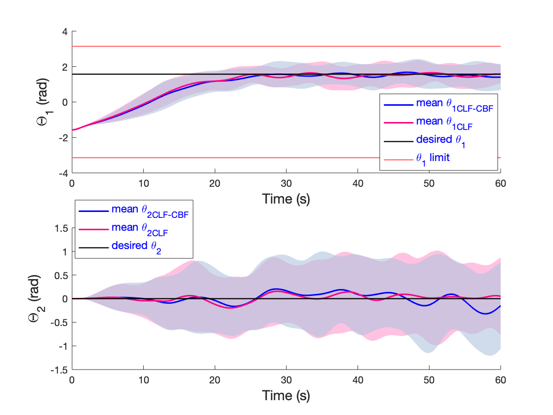
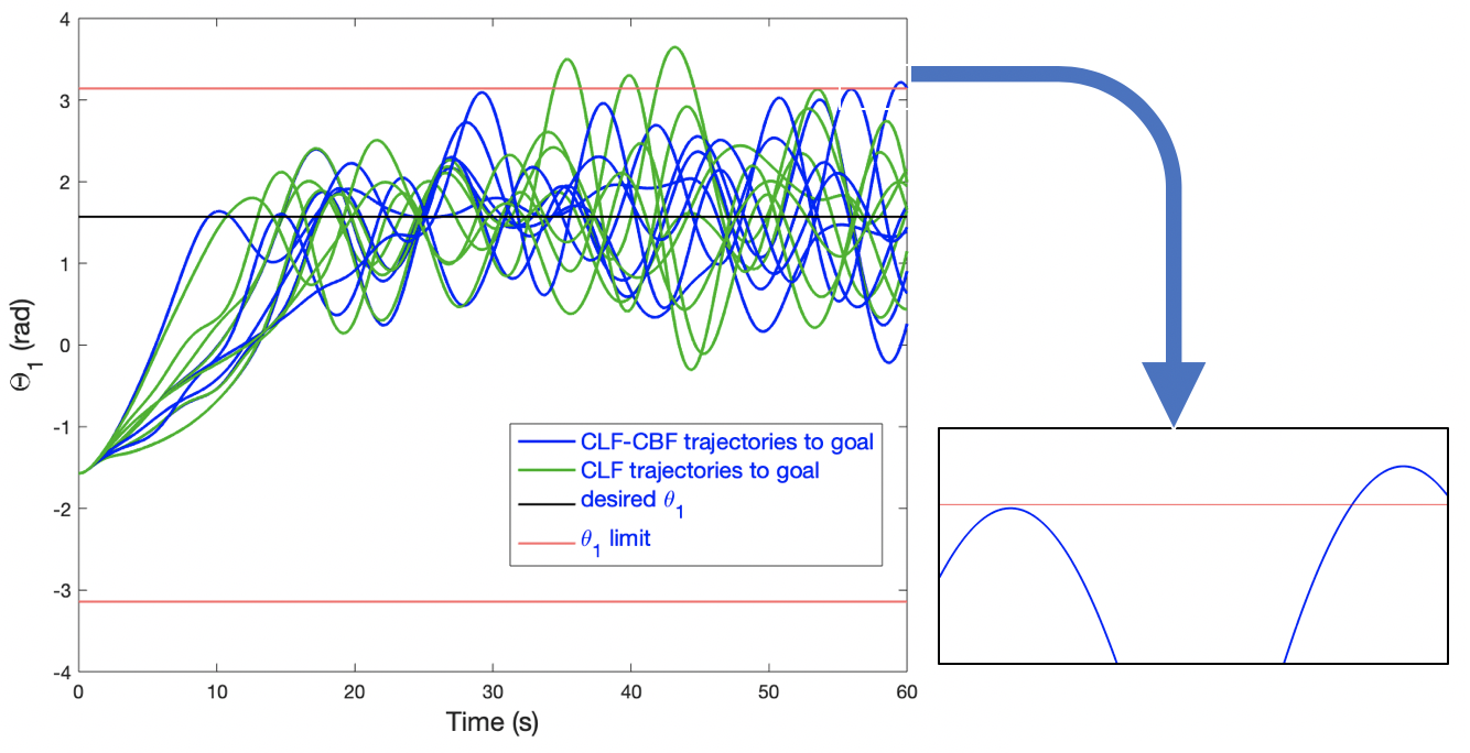
We simulated 40 sample trajectories for a time horizon of 60s. σ=0.05𝜎0.05\sigma=0.05, d=1000𝑑1000d=1000 and Q𝑄Q was taken as Identity. The results from the simulations are presented in figure 3 and figure 4.From our experiments we found that since the proposed method essentially solves a QP, it is highly dependent on how efficiently the optimizer can converge to a feasible solution. The highlighted portion in figure 4 shows one such cases where the optimizer fails to converge to a feasible solution and thus the trajectories violates the safety constraints.
Refer to caption
Figure 3: 2-Link pendulum task: The mean and the sigma distribution of the θ1subscript𝜃1\theta_{1} and θ2subscript𝜃2\theta_{2} state trajectories for the CLF-CBF controller and the CLF controller are plotted here in sheds of blue and green respectively.
Refer to caption
Figure 4: 2-Link pendulum task: 7 test trajectories out of the 40 sample trajectories for θ1subscript𝜃1\theta_{1} are shown here. The green ones generated with the CLF controller violates the constraint conditions where as the blue ones from the CLF-CBF controller successfully stays between the πθ1π𝜋subscript𝜃1𝜋-\pi\leq\theta_{1}\leq\pi bounds. The highlighted case shows the scenario where the optimizer fails to find a feasible solution and violates the boundary conditions.

VII Conclusion and Future Work

We have introduced a generalised framework for control Lyapunov and barrier functions for stochastic systems with high relative degree. We have provided the necessary condition to guarantee asymptotic stability in the sense of probability to stochastic systems with observable states that are not directly actuated via control. Our high relative degree SCBF framework ensure safety bounds to a system by providing a means to incorporate positional state dependent constraints into the control problem formulation. Our control policies are evaluated in the form of a QP which has state dependent constraints based on SCLF-SCBF conditions. We have demonstrated the effectiveness of our proposed control methodology with numerical studies on a relative degree 2 system (2D car navigation with multiple obstacles) and 4 system (2-link pendulum with elastic actuator swing task).

The present work opens up numerous application of stochastic CLF and CBF formulation to safety critical systems. This formulation will be of particular interest to explore safe and sample efficient Reinforcement Learning frameworks that can incorporate the safety bounds in the formulation of the optimisation problem itself rather than learning them from making mistakes.

References

  • [1] Q. Nguyen and K. Sreenath, “Exponential control barrier functions for enforcing high relative-degree safety-critical constraints,” in 2016 American Control Conference (ACC), pp. 322–328, IEEE, 2016.
  • [2] M. Althoff, C. Le Guernic, and B. H. Krogh, “Reachable set computation for uncertain time-varying linear systems,” in Proceedings of the 14th International Conference on Hybrid Systems: Computation and Control, HSCC ’11, (New York, NY, USA), p. 93–102, Association for Computing Machinery, 2011.
  • [3] S. Mitra, T. Wongpiromsarn, and R. M. Murray, “Verifying cyber-physical interactions in safety-critical systems,” IEEE Security Privacy, vol. 11, no. 4, pp. 28–37, 2013.
  • [4] A. D. Ames, J. W. Grizzle, and P. Tabuada, “Control barrier function based quadratic programs with application to adaptive cruise control,” in 53rd IEEE Conference on Decision and Control, pp. 6271–6278, IEEE, 2014.
  • [5] A. D. Ames, S. Coogan, M. Egerstedt, G. Notomista, K. Sreenath, and P. Tabuada, “Control barrier functions: Theory and applications,” in 2019 18th European Control Conference (ECC), pp. 3420–3431, IEEE, 2019.
  • [6] A. Clark, “Control barrier functions for complete and incomplete information stochastic systems,” in 2019 American Control Conference (ACC), pp. 2928–2935, IEEE, 2019.
  • [7] W. Xiao and C. Belta, “Control barrier functions for systems with high relative degree,” CoRR, vol. abs/1903.04706, 2019.
  • [8] H. Deng and M. Krstić, “Stochastic nonlinear stabilization—ii: inverse optimality,” Systems & control letters, vol. 32, no. 3, pp. 151–159, 1997.
  • [9] Y. Nishimura, K. Tanaka, Y. Wakasa, and Y. Yamashita, “Stochastic asymptotic stabilizers for deterministic input-affine systems based on stochastic control lyapunov functions,” IEICE Transactions on Fundamentals of Electronics, Communications and Computer Sciences, vol. 96, no. 8, pp. 1695–1702, 2013.
  • [10] Y. Wang and S. Boyd, “Performance bounds for linear stochastic control,” Systems & Control Letters, vol. 58, no. 3, pp. 178–182, 2009.
  • [11] R. Khasminskii, Stochastic stability of differential equations, vol. 66. Springer Science & Business Media, 2011.
  • [12] D. D. Fan, J. Nguyen, R. Thakker, N. Alatur, A.-a. Agha-mohammadi, and E. A. Theodorou, “Bayesian learning-based adaptive control for safety critical systems,” arXiv preprint arXiv:1910.02325, 2019.
  • [13] E. Todorov and W. Li, “A generalized iterative lqg method for locally-optimal feedback control of constrained nonlinear stochastic systems,” in Proceedings of the 2005, American Control Conference, 2005., pp. 300–306, IEEE, 2005.
  • [14] M. A. Pereira, Z. Wang, I. Exarchos, and E. A. Theodorou, “Learning deep stochastic optimal control policies using forward-backward sdes,” in Robotics: science and systems, 2019.
  • [15] I. Exarchos and E. A. Theodorou, “Stochastic optimal control via forward and backward stochastic differential equations and importance sampling,” Automatica, vol. 87, pp. 159–165, 2018.
  • [16] Z. Xie, C. K. Liu, and K. Hauser, “Differential dynamic programming with nonlinear constraints,” in 2017 IEEE International Conference on Robotics and Automation (ICRA), pp. 695–702, 2017.