Sequential Design of Mixture Experiments with an Empirically Determined Input Domain and an Application to Burn-up Credit Penalization of Nuclear Fuel Rods

Abstract

This paper proposes a sequential design for maximizing a stochastic computer simulator output, $y(\bm{x})$, over an unknown optimization domain. The training data used to estimate the optimization domain are a set of (historical) inputs, often from a physical system modeled by the simulator. Two methods are provided for estimating the simulator input domain. An extension of the well-known efficient global optimization algorithm is presented to maximize $y(\bm{x})$. The domain estimation/maximization procedure is applied to two readily understood analytic examples. It is also used to solve a problem in nuclear safety by maximizing the k-effective “criticality coefficient” of spent fuel rods, considered as one-dimensional heterogeneous fissile media. One of the two domain estimation methods relies on expertise-type constraints. We show that these constraints, initially chosen to address the spent fuel rod example, are robust in that they also lead to good results in the second analytic optimization example. Of course, in other applications, it could be necessary to design alternative constraints that are more suitable for these applications.

KEY WORDS: Expected Improvement; Gaussian process interpolator; Simplex; Stochastic simulation; Unknown input domain.

1 Introduction

Among the important issues in safety assessment is the prevention of accidental events. In nuclear safety applications, there are at least two ways of minimizing potential accidental events: the identification of worst cases (and then averting of such cases), and the probabilistic containment of accident consequences. Depending on the application, the opportunity to choose one or the other method can rely on practical considerations, but should be a consistent part of the whole safety framework and include information from many fields (say, for example, seismology, structural mechanics, nuclear core cooling, neutronics, and radiology).

Common industrial applications have fewer uncontrollable external conditions than applications subject to environmental factors. Indeed, sophisticated mathematical models of industrial safety studies are ordinarily regarded as reliable descriptions of their performance in the real-world. Thus, many industrial safety studies use mathematical models of the industrial process to identify and then avoid worst-case scenarios.

However when the complexity of the safety study increases and the mathematical model is sensitive to uncertain parameters, the prevention of mathematically-determined unacceptable events becomes a less reliable method of preventing accidental events. A typical example of increasing system complexity occurs when the known homogeneity of a critical materials’ density, its mixing phases, its temperature, or other spatially-dependent properties can not be guaranteed to be assumed fixed values. To more accurately approximate reality, the homogeneous model of critical components must be replaced by an imperfectly-known, heterogeneous one. However, it is typically far more difficult to determine the worst case performance of a system having heterogeneous components than systems having known subsystems.

This paper proposes methodology to provide a worst-but-credible-case for imperfectly known heterogeneous models. The methodology is illustrated in analytical examples and in an application to nuclear fuel storage. In the latter example, an assessment is made of the stability of fissile fuel rods after their previous use in a nuclear reactor (their “burn-up credit”) in order to relax their storage requirements. Fissile fuel rods identified as more stable can be stored in a reduced-risk facility.

The goals of this paper are two-fold. First, it estimates the (optimization) domain ${\cal X}$ of inputs “consistent” with a training set of inputs, say $\bm{x}_{1},\ldots,\bm{x}_{n}$, possibly historical data from a physical system with the same domain as the simulator. Second, it identifies an $\bm{x}^{\star}\in{\cal X}$ that maximizes $y(\bm{x})$ over $\bm{x}\in{\cal X}$.

The literature contains a number of papers that provide additional relevant background useful to more fully understand the nuclear safety example and the statistical optimization of stochastic simulators. Cacuci (2010) provides basic grounding on nuclear engineering and on the numerical simulation for such applications. Stinstra et al. (2003) and Draguljić et al. (2012) propose statistical methodology for constructing input designs for simulators that have bounded polygonal input domains. de Klerk (2008) reviews the optimization of a deterministic function defined on a simplex. Picheny et al. (2013) estimate sequentially the quantile of a function $y(\bf{X})$ with random inputs $\bm{X}$ when $y(\bf{x})$ is observed with measurement error.

The remainder of this paper is organized as follows. Section 2 states the mathematical notation used to formally describe the problems solved in subsequent sections of the paper. Section 3 reviews the Efficient Global Optimization (EGO) of Jones et al. (1998) for minimizing an unknown $y(\bm{x})$ $:\mathcal{X}\mapsto\mathbb{R}$ over a rectangular $\mathcal{X}$ and modifications of EGO for cases when $y(\bm{x})$ is measured with noise. Section 4 introduces two methods for identifying a set of inputs $\bm{x}$ that are compatible with the training inputs. One method, given in Subsection 4.1, uses expert-type constraints and a second method, described in Subsection 4.2, uses a kernel density estimation approach. Finally, Section 5 gives three examples; the first is an easily understood analytic application which is used to observe the performance of the proposed methodology; the second is a determination of configurations of spent fuel rods in nuclear power reactors that are associated with high criticality settings and the third is an analytical example that illustrates the robustness and generalizability of the global methodology.

2 Mathematical Description of the Optimization Problem

First, the mathematical notation and assumptions will be stated and then the nuclear safety application will be stated to illustrate the notation. Consider a real-valued (simulator) $y(\bm{\cdot})$ having functional input $x(t)$; $x(t)$ is assumed to be positive and continuous with argument $t$ having domain that is a bounded interval that is taken to be $[0,1]$, possibly after a location shift and scale transformation. Let $\bm{x}$ denote the input function $\{x(t)\}_{t\in[0,1]}$. In our nuclear safety application, all inputs $\bm{x}$ are assumed to come from a domain determined by a training set of inputs to a physical system that is described below in more detail. The simulator output at input $\bm{x}$ is $y(\bm{x})$ corrupted by an additive measurement error.

Two other features of the input functions that are consistent with nuclear safety study will be assumed. First, all inputs $x(t)$ are measured at a common finite grid of $d$ values, say, $0\leq t_{1}<\cdots<t_{d}\leq 1$. This grid is assumed to be the same for all functions. A linear, quadratic or other interpolation scheme would be applied to the available $x(t)$ measurements to achieve a common $t$ grid if this is not true on their native scale. Because of their origin, this paper will refer to the $d\times 1$ vector $\bm{x}=\left(x(t_{1}),\ldots,x(t_{d})\right)^{\top}$ as a curve or a function. Second, by dividing each component of $\bm{x}$ by its mean $\bar{x}=\frac{1}{d}\sum_{j=1}^{d}x(t_{j})$ it is assumed that $\sum_{j=1}^{d}x(t_{j})=d$ for all inputs. Thus the set of valid inputs is a subset of the positive $d$-hyperplane, i.e., of $\left\{(w_{1},\ldots,w_{d}):w_{j}\geq 0\mbox{\ for }j=1,\dots,d;\sum_{j=1}^{d}w_{j}=d\right\}$. Equivalently, the $d\times 1$ vector $\bm{x}$ has non-negative discrete values whose average is one.

To illustrate the notation of the previous two paragraphs for the nuclear safety application, consider spent fuel rods that are retrieved from a nuclear reactor and inspected. These rods are modeled as one-dimensional heterogeneous fissile media. Here $x(t)$ is the “burn-up rate” (in megawatt-days/ton) measured at vertical position $t$ along the fuel rod, where the rod is scaled so that $t\in[0,1]$. Remark that the fuel rods are considered for storage at a fixed time, thus the burn-up rate is considered to depend only on the position and not on the time. Figure 1 is a cartoon that illustrates a spent fuel rod and the corresponding burn-up rate energy $x(t)$. In this application we have available $n=$ 3,158 spent fuel rods (and their burn-up rate curves) from standard nuclear power plants, (Cacciapouti and Volkinburg (1997)). The burn-up rate is measured at $d=18$ equally-spaced points along $[0,1]$. Let $\bm{x}_{i}=\left(x_{i}(t_{1}),\ldots,x_{i}(t_{18})\right)^{\top}$, $i=1,\ldots,$ 3,158 denote the burn-up rate curves for the spent fuel rods. Each $\bm{x}_{i}$ is an element of the positive $18$-hyperplane.

For any input $\bm{x}$, the associated simulator output $y(\bm{x})$ is the criticality coefficient at $\bm{x}$. The criticality coefficient is computed from depletion calculations made for each of the $d=18$ zones of the rod based on macroscopic cross-sections. The zone-specific determinations are made using the numerical simulation package CRISTAL (CRISTAL, 2018) and is followed by a Monte-Carlo $k$-effective calculation for the entire burn-up rate curve. The $y(\bm{x})$ value is interpreted as follows: if $y(\bm{x})<1$, the rod is called “subcritical”; if $y(\bm{x})=1$, the rod is “critical”; and if $y(\bm{x})>1$, the rod is termed “super-critical”. In particular, an higher value of $y(\bm{x})$ corresponds to more risk and thus the goal is to maximize $y(\bm{x})$, for safety study.

Figure 1: Schematic of a spent fuel rod and its burn-up rate curve.

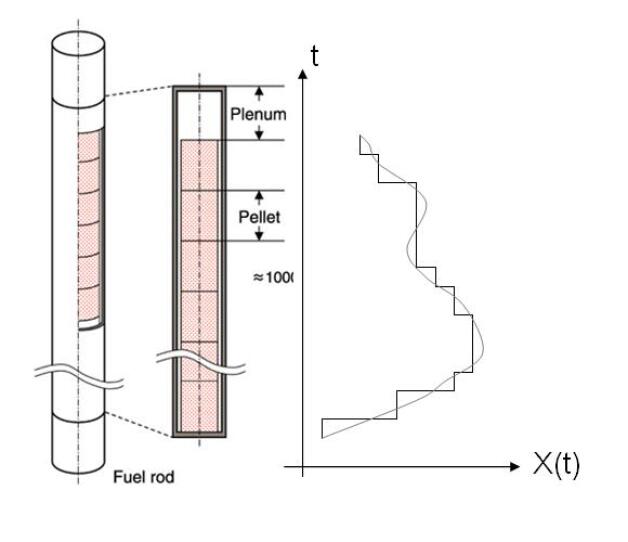
Unfortunately, the observed value of the criticality coefficient is a noisy version of $y(\bm{x})$. In addition, CRISTAL can be costly to run although, in this application, the evaluations are approximately 15 minutes each. Let $y_{i}=y(\bm{x}_{i})$ denote the observed computed criticality coefficient for the $i^{th}$ spent fuel rod, $i=1,\ldots,$ 3,158.

3 Sequential Optimization

Section 4 will describe two methods for constructing an input domain ${\cal X}$ that is consistent with historical input data to the desired physical system. This section will review the “expected improvement” sequential designs of Schonlau et al. (1998) and Jones et al. (1998) that were introduced to minimize a deterministic $y(\bm{x})$ when evaluations are costly. Called Efficient Global Optimization (EGO) algorithms these designs seek to find an $x_{\min}\in\arg\min_{\bm{x}\in\mathcal{X}}y(\bm{x})$. The problem of maximizing $y(\bm{x})$ can be solved by applying EGO to minimize $-y(\bm{x})$. Additional modifications will be given to handle cases when $y(\bm{x})$ is measured with error.

In brief, EGO is initiated by computing $y(\bm{x})$ on a space-filling set of inputs of ${\cal X}$. Thus initial information about $y(\bm{\cdot})$ is available over a wide, if not dense, subset of the input space.

At each update step, EGO adds one input $\bm{x}\in{\cal X}$ to the previous design and the associated $y(\bm{x})$ to the output vector. Suppose that there have been previous evaluations at $y(\bm{x}_{1})$, …, $y(\bm{x}_{n})$. EGO identifies the next input at which to evaluate $y(\bm{\cdot})$, denoted $\bm{x}_{n+1}$, as the $\bm{x}$ which maximizes the idealized improvement function

$${\cal I}(\bm{x})=\left\{\begin{array}[]{ll}y_{\min}^{n}-y(\bm{x}),&y_{\min}^{n}-y(\bm{x})>0\\[4.30554pt] 0,&y_{\min}^{n}-y(\bm{x})\leq 0\end{array}\right.$$ (1)

where $y_{\min}^{n}=\min_{i=1,\ldots,n}y(\bm{x}_{i})$ is the smallest value of $y(\bm{x})$ among the previous evaluations. Intuitively, larger values of ${\cal I}(\bm{x})$ produce smaller values of $y(\bm{x})$.

While $y_{\min}^{n}$ is known, both $y(\bm{x})$ and hence ${\cal I}(\bm{x})$ are unknown. EGO uses a Gaussian process extension of the regression predictor to estimate $y(\bm{x})$ by $\widehat{y}(\bm{x})$ say, and to quantify the uncertainty in this predictor by $s(\bm{x})$, say (See Schonlau et al. (1998) or Chapter 3 of Santner et al. (2018)). This stochastic approximation can be used to find a formula for the expected value of a stochastic version of ${\cal I}(\bm{x})$ given the current data. The resulting (practical) improvement function is

$$EI\left[(\bm{x})\right]=(y_{\min}^{n}-\widehat{y}(\bm{x}))\,\Phi\left(\frac{y_{\min}^{n}-\widehat{y}(\bm{x})}{s(\bm{x})}\right)+s(\bm{x})\,\phi\left(\frac{y_{\min}^{n}-\widehat{y}(\bm{x})}{s(\bm{x})}\right),$$ (2)

where $\Phi(\bm{\cdot})$ and $\phi(\bm{\cdot})$ are the $N(0,1)$ distribution and density function, respectively.

EGO is typically stopped after a fixed budget has been exhausted for $y(\bm{x})$ evaluations or when the maximum expected improvement is “small”. When EGO stops sampling, it predicts $\bm{x}_{\min}$ to be that member of the current set of inputs at which $y(\bf{\cdot})$ has been evaluated, say $\{\bm{x}_{1},\ldots,\bm{x}_{N}\}$, to satisfy

$$y(\widehat{\bm{x}}_{\min})=\min_{i=1,\ldots,{N}}y(\bm{x}_{i})\,.$$ (3)

The article by Picheny et al. (2013) and the references therein discuss extensions of EGO to sequentially identify an $\bm{x}\in\arg\min y(\bf{x})$ when $y(\bm{x})$ observations contain measurement error, i.e., when the observed value at $\bm{x}$ is

$$y^{o}(\bf{x})=y(\bf{x})+\epsilon(\bf{x}),$$

where $\epsilon(\bf{x})$ is a white noise process with variance ${\tau^{2}}$. In this case, various approximations of the unobserved $y_{\min}^{n}$ have been suggested, including the standard plugin approach where $y_{\min}^{n}$ is approximated by $y_{\min}^{n}=\min_{i=1,\ldots,n}\hat{y}(\bm{x}_{i})$, see Picheny et al. (2013) and references therein. Here we approximate $y_{\min}^{n}$ by $\min_{i=1,\ldots,n}\hat{y}(\bm{x}_{i})-2\tau$, where $\tau$ is the noise standard deviation. Indeed, decreasing $y_{\min}^{n}$ in (2) typically increases the value of the expected improvement at input points with large uncertainties and large predictions, compared to points with small uncertainties and small predictions. Hence, this promotes exploration. Furthermore, the choice of the factor $-2$ is consistent with the common practice in nuclear safety of penalizing Monte Carlo simulation results by taking $5\%$ or $95\%$ Gaussian quantiles.

In this paper the problem of maximizing $y(\bm{x})$ over $\bm{x}$ in an unknown ${\cal X}$ is solved by identifying ${\cal X}$ using one of the two methods described in Section 4. Then the problem

$$\bm{x}^{\star}\in\operatorname*{argmax}_{\bm{x}\in{\cal X}}y(\bm{x})$$ (4)

is solved by the stochastic version of the EGO algorithm. Because the empirically determined optimization domains for both examples in Section 5 are subsets of hyperplanes, the following adjustment is made. The EGO algorithm is applied to maximize the expected improvement over $\bm{x}\in E$ where $E=\bm{\Lambda}{\cal X}$ and the linear transformation $\bm{\Lambda}$ is stated in Loeppky et al. (2013). The dimension of $E$ is one less than the number of components of $\bm{x}\in{\cal X}$.

4 Empirical Determination of the Input Domain

This section describes two methods for identifying a set of positive input curves $\bm{x}=(x_{1},\ldots,x_{d})^{\top}$ which satisfy $\sum_{j=1}^{d}x_{j}=d$ and that are “near” the historical set of curves, $\bm{x}_{i}=\left(x_{i,1},\ldots,x_{i,d}\right)^{\top}$, $i=1,\ldots,n$. These constructions recognize that the historical curves form a skeleton of the total set of curves that should be considered as the input domain for the optimization problems considered in this paper. Informally, we use the notation $\mathcal{X}$ to denote the input space. The first approach introduced in this section defines $\mathcal{X}$ by constraints based on a mixture of expert knowledge of the physical system and/or graphical analysis of $\bm{x}_{1},\ldots,\bm{x}_{n}$. The second approach defines $\mathcal{X}$ as a kernel density estimate formed from the coefficients of the projections of the historical $\bm{x}_{i}$ onto a basis of spline functions.

4.1 Defining $\mathcal{X}$ Using Expert Knowledge and/or Empirical Experience

The first approach identifies $\mathcal{X}$ to be positive $\bm{x}$ curves using constraints determined by expert knowledge and/or empirical experience. The latter uses a visual analysis of the $n$ historical curves. As an example, the following four constraints based on the historical data were used in the examples of Section 5.

1. Bound Constraints at each of the $d$ component positions of $\bm{x}$

$$\min_{i=1,\ldots,n}({x}_{i,j})-\epsilon\leq x_{j}\leq\max_{i=1,\ldots,n}({x}_{i,j})+\epsilon$$ (5)

where $j\in\{1,\ldots,d\}$ and $\epsilon\geq 0$ is a user-specified tolerance level.

2. Bounds on Incremental Changes in consecutive components of $\bm{x}$

$$\min_{i=1,\ldots,n}\left[{x}_{i,j+1}-{x}_{i,j}\right]-\epsilon\leq x_{j+1}-x_{j}\leq\max_{i=1,\ldots,n}\left[{x}_{i,j+1}-{x}_{i,j}\right]+\epsilon$$ (6)

for all $j\in\{1,\ldots,d-1\}$ where $\epsilon>0$ is a user-specified tolerance level.

3. Constraints on Maximum Variation of $\bm{x}$

$$\max_{j=j_{1},\ldots,j_{2}}|x_{j+1}-x_{j}|\leq\max_{i=1,\ldots,n}\max_{j=j_{1},\ldots,j_{2}}|{x}_{i,j+1}-{x}_{i,j}|+\epsilon,$$ (7)

where $1\leq j_{1}<j_{2}\leq d$ and $\epsilon\geq 0$ are user-specified.

4. Constraints on Maximum Total Variation of $\bm{x}$

$$\sum_{j=j_{1}}^{j_{2}}|x_{j+1}-x_{j}|\leq\max_{i=1,\ldots,n}\sum_{j=j_{1}}^{j_{2}}|{x}_{i,j+1}-{x}_{i,j}|+\epsilon,$$ (8)

where $1\leq j_{1}<j_{2}\leq d$ and $\epsilon\geq 0$ are user-specified. In other cases, more general linear or non-linear constraints such as

$$\bm{A}\begin{bmatrix}\bm{x}_{i}\\ \bm{x}\end{bmatrix}{\color[rgb]{0,0,0}\leq}\ \bm{b}$$

for $i=1,\ldots,n$, or

$$\begin{bmatrix}f_{1}(\bm{x}_{1},\ldots,\bm{x}_{n},\bm{x})\\ \vdots\\ f_{s}(\bm{x}_{1},\ldots,\bm{x}_{n},\bm{x})\end{bmatrix}\leq\begin{bmatrix}b_{1}\\ \vdots\\ b_{s}\end{bmatrix}$$

could be used. We remark that the contraints 1 and 2 above are linear with respect to $\bm{x}$, while the constraints 3 and 4 are non-linear with respect to $\bm{x}$.

4.2 Defining $\mathcal{X}$ by Projections onto a Basis Set

Projecting $x(t)$ onto the Set of Spline Basis Functions

The references Ramsay (2006) and Muehlenstaedt et al. (2017) provide an introduction to spline basis functions. Let $\mathbb{N}$ denote the set of positive integers. Briefly, a spline basis of order $m$, $m\in\mathbb{N}$, is a set of functions $B_{i,m}:[0,1]\to\mathbb{R}^{+}$, for $i=1,\ldots,K$ where $K\in\mathbb{N}$ is the number of spline functions. Here $m$ is called the order of the spline. Figure 2 illustrates the notation.

Figure 2: $K=8$ spline functions of order $5$; each spline can be identified by the location of its maximum value.

The projection of a given positive real-valued function $x$$:$ $[0,1]\to\mathbb{R}^{+}$ onto $\{B_{i,m}(t)\}_{i=1}^{K}$ is the function

$$\widehat{x}^{(m,K)}=\widehat{x}^{(m,K)}(t)=\frac{\widetilde{x}^{(m,K)}(t)}{(1/d)\sum_{j=1}^{d}\widetilde{x}^{(m,K)}(t_{j})}$$

where

$$\widetilde{x}^{(m,K)}(t)=\sum_{k=1}^{K}\alpha^{\star}_{k}B_{k,m}(t),\ \ \mbox{and}\ (\alpha^{\star}_{1},\ldots,\alpha^{\star}_{K})\in\operatorname*{argmin}_{\alpha\in\mathbb{R}^{K}}\int_{0}^{1}\left(x(t)-\sum_{i=1}^{K}\alpha_{i}B_{i,m}(t)\right)^{2}dt$$ (9)

which shows that $\widehat{x}^{(m,K)}$ has the form

$$\widehat{x}^{(m,K)}(t)=\sum_{k=1}^{K}\widehat{\alpha}_{k}B_{k,m}(t).$$ (10)

The coefficients $\bm{\alpha}^{\star}=(\alpha^{\star}_{1},\ldots,\alpha^{\star}_{K})$ have an explicit expression as the least square solution to (9) and hence ${\widehat{\bm{\alpha}}}=(\widehat{\alpha}_{1},\ldots,\widehat{\alpha}_{K})$ is straightforward to obtain.

Recall that the observed data for the $i^{th}$ curve is the vector $\bm{x}_{i}=(x_{i}(t_{1}),\ldots,x_{i}(t_{d}))^{\top}$, $i=1,\ldots,n$. To apply (9) to the function $\bm{x}=\bm{x}_{i}$, let $\phi_{i}$ denote the spline interpolating function satisfying $\phi_{i}(t_{1})=x_{i}(t_{1}),\dots,\phi_{i}(t_{d})=x_{i}(t_{d})$. Then $\bm{\alpha}^{\star}$ corresponding to $\bm{x}_{i}$ is obtained from (9) by replacing $x(t)$ by $\phi_{i}(t)$. (In the Section 5 examples, $\phi_{i}(t)$ is obtained by the R function splinefun in the package splines.)

Kernel Density Estimation

Let $\widehat{\bm{\alpha}}^{(i)}=\left(\widehat{\alpha}^{(i)}_{1},\ldots,\widehat{\alpha}^{(i)}_{K}\right)$ denote the $(\widehat{\alpha}_{1},\ldots$,$\widehat{\alpha}_{K})$ in (10) for the $i^{th}$ input curve $\bm{x}_{i}$, $i=1,\ldots,n$. Consider the following kernel density estimation procedure based on the set $\left\{\widehat{\bm{\alpha}}^{(1)},\ldots\right.$, $\left.\widehat{\bm{\alpha}}^{(n)}\right\}$. Following the approach of Perrin et al. (2018), let $\phi(\bm{\cdot})$ denote the probability density function of the univariate standard Normal distribution. Given $K$ and positive scale factors $\bm{\lambda}=\left(\lambda_{1},\ldots,\lambda_{K}\right)$, let

$$\rho_{\lambda_{1},\ldots,\lambda_{K}}(\bm{\alpha})=\rho_{\bm{\lambda}}(\bm{\alpha})=\frac{1}{n}\sum_{i=1}^{n}\prod_{k=1}^{K}\frac{1}{\lambda_{k}}\phi\left(\frac{\alpha_{k}-\widehat{\alpha}^{(i)}_{k}}{\lambda_{k}}\right)$$ (11)

define a function from $\mathbb{R}^{K}$ to $\mathbb{R}^{+}$ where $\bm{\alpha}=(\alpha_{1},\ldots,\alpha_{K})$. It is straightforward to check that $\rho_{\bm{\lambda}}(\bm{\alpha})$ has integral one over $\mathbb{R}^{K}$. Intuition suggests that given a scaling $\bm{\lambda}\in(0,\infty)^{K}$, $\rho_{\bm{\lambda}}(\bm{\alpha})$ is large for choices of $\bm{\alpha}$ that are compatible with the set of observed input curves.

In this paper the scale parameters $\lambda_{1},\ldots,\lambda_{K}$ are selected by cross validation using

$$\widehat{\bm{\lambda}}=(\widehat{\lambda}_{1},\ldots,\widehat{\lambda}_{K})^{\top}\in\operatorname*{argmax}_{(\lambda_{1},\ldots,\lambda_{K})\in(0,\infty)^{K}}\sum_{i=1}^{n}\log\left(\rho^{-i}_{\bm{\lambda}}(\widehat{\bm{\alpha}}^{(i)})\right)$$ (12)

where $\rho^{-i}_{\bm{\lambda}}$ is obtained from (11) by removing $\widehat{\bm{\alpha}}^{(i)}$ from the set $\left\{\widehat{\bm{\alpha}}^{(i)}\right\}_{i=1}^{n}$ (and decrementing $n$ to $n-1$). Thus $\rho_{\widehat{\bm{\lambda}}}(\bm{\alpha})$ can be viewed as a kernel density estimator most compatible with the coefficients $\left\{\widehat{\bm{\alpha}}^{(1)},\ldots\right.$, $\left.\widehat{\bm{\alpha}}^{(n)}\right\}$ from $\bm{x}_{1}$, …, $\bm{x}_{n}$. Thus the value of $\rho_{\widehat{\bm{\lambda}}}(\bm{\alpha})$ is used to quantify the level of “realism” of curves having form $\sum_{k=1}^{K}\alpha_{k}B_{k,m}$ to the observed $\bm{x}_{1}$, …$\bm{x}_{n}$.

Threshold Selection

In the following, $\widehat{\rho}(\bm{\alpha})=\rho_{\widehat{\bm{\lambda}}}(\bm{\alpha})$ denotes the estimated compatibility function in (11) and (12). To select discretized curves $\bm{x}$ most compatible with the training data, we choose $T>0$ such that $\bm{\alpha}\in\mathbb{R}^{K}$ is considered compatible with $\bm{x}_{1},\ldots,\bm{x}_{n}$ if and only if $\widehat{\rho}(\bm{\alpha})\geq T$.

The value $T$ is chosen as follows. For $\bm{\alpha}\in\mathbb{R}^{K}$, let $x_{\bm{\alpha}}(t)=\sum_{k=1}^{K}{\alpha}_{k}B_{k,m}(t)$; given $\Delta~{}>~{}0$, select a $T>0$ such that any $\bm{\alpha}$ which satisfies

$$\left(\int_{0}^{1}\left[x_{\bm{\alpha}}(t)-x_{\widehat{\bm{\alpha}}^{(i)}}(t)\right]^{2}dt\right)^{1/2}\leq\Delta$$ (13)

for at least one $i\in\{1,\ldots,n\}$ also satisfies $\widehat{\rho}(\bm{\alpha})\geq T$. Inspection of (11) shows that $\widehat{\rho}(\bm{\alpha})\geq T$ holds provided, for some $i\in\{1,\ldots,n\}$,

$$\frac{1}{n}\prod_{k=1}^{K}\frac{1}{\widehat{\lambda}_{k}}\phi\left(\frac{\alpha_{k}-\widehat{\alpha}^{(i)}_{k}}{\widehat{\lambda}_{k}}\right)\geq T$$ (14)

and (13) holds for this $\bm{\alpha}$ and $i$. The expression on the right hand side of (14) is the limiting value of (11) corresponding to the case where $\widehat{\bm{\alpha}}^{(i)}$ is infinitely distant from all $\{\widehat{\bm{\alpha}}^{(\ell)}\}_{\ell\neq i}$ and where $\left(\int_{0}^{1}\left[x_{\bm{\alpha}}(t)-x_{\widehat{\bm{\alpha}}^{i}}(t)\right]^{2}dt\right)^{1/2}\leq\Delta$. Based on the above observations, the selected threshold $\widehat{T}$ is defined as

$$\widehat{T}=\min_{\begin{subarray}{c}\bm{\alpha}\in\mathbb{R}^{K}\\ \left(\int_{0}^{1}x_{\bm{\alpha}}(t)^{2}dt\right)^{1/2}\leq\Delta\end{subarray}}\frac{1}{n}\prod_{k=1}^{K}\frac{1}{\widehat{\lambda}_{k}}\phi\left(\frac{\alpha_{k}}{\widehat{\lambda}_{k}}\right).$$ (15)

In practice, the calculation of $\widehat{T}$ in (15) is straightforward since one can precompute the Gram matrix with $(i,j)^{th}$ element $\int_{0}^{1}B_{i,m}(t)B_{j,m}(t)dt$.

Let $\bm{x}(\bm{\alpha})$ denote the $d\times 1$ vector with $j^{th}$ element $\left[\sum_{k=1}^{K}\alpha_{k}B_{k,m}(t_{j})\right]$ for $j=1,\ldots,d$. As for the historical data, scaling $\bm{x}(\bm{\alpha})$ by the average of its components, i.e., by $\bar{x}(\bm{\alpha})=(x_{1}(\bm{\alpha})+\ldots+x_{d}(\bm{\alpha}))/d$ results in a positive point on the $d$-hyperplane (when $\bm{\alpha}$ has positive components). To select $\bm{\alpha}$ compatible with $\widehat{\rho}(\bm{\alpha})>T$, compute

$$\bm{\alpha}^{*}\in\operatorname*{argmax}_{\begin{subarray}{c}\bm{\alpha}\in[0,\infty)^{K}\\ \widehat{\rho}(\bm{x}(\bm{\alpha})/\bar{x}(\bm{\alpha}))\geq\Delta\\ \end{subarray}}y(\bm{x}(\bm{\alpha})/\bar{x}(\bm{\alpha})).$$ (16)

The optimization problem corresponds to minimizing a function where the constraints can be tested with negligible cost. This optimization takes place in the $K$-dimensional space of the $\bm{\alpha}^{\prime}s$.

5 Worked Examples

The rationale behind our approaches to forming an optimization domain, i.e., using expert-determined constraints or projections, relies on the availability of a sufficient amount of relevant data. Following an explanatory data analysis (EDA) of the burn-up profile data in Section 5.1, Section 5.2 applies both methods to identify a set of burn-up rate curves $\bm{x}$ that are consistent with those of spent fuel rods from nuclear plants based of the “historical” curves in the axial burn-up profile database for pressurized water reactors available through OECD Nuclear Energy Agency Data Bank (Cacciapouti and Volkinburg, 1997).

Subsection 5.3 applies the optimization method of Section 3 to a simple analytic function where the answer and the performance of the optimization procedure is straightforward to understand. Then Subsection 5.4 considers the example introduced in Section 2 to maximize the criticality coefficient for spent fuel rods. This process is termed Burn-up Credit Penalization in the nuclear industry. Finally, Subsection 5.5 discusses the generalizability of the methodology of this paper. It presents an additional analytical example where both the historical curves and the objective function are unknown.

5.1 Exploratory Analysis of the Fuel Rod Data

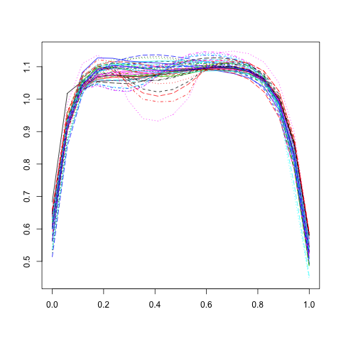
In this application, there are $n=$ 3,158 discretized burn-up rate curves $\bm{x}_{1}$, …, $\bm{x}_{3158}$, each of which has been measured at the (same) $d=18$ vertical measurement points $(0,1/17$,…, $16/17,1)$. Recall that the curves have been normalized so that $\sum_{j=1}^{18}x_{i,j}=18$, for $i=1,\ldots,$ 3,158, or equivalently to have an average burn-up rate equal to one. Figure 3 shows $50$ representative curves from the population of curves; all $50$ curves show a common ‘vertical-horizontal-vertical’ shape which is true of the majority of curves. A small minority of the population have a more complex character.

Figure 3: Fifty representative burn-up rate curves from the population of 3,158 discretized historical curves.

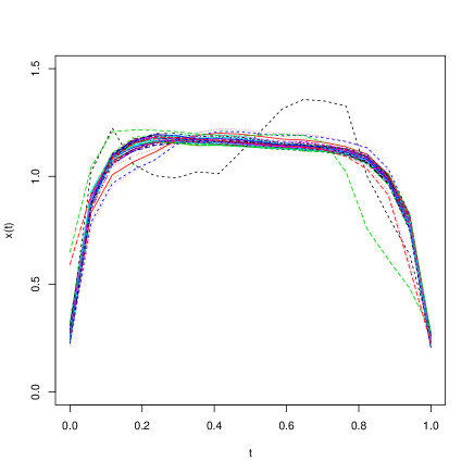
Because each run of the CRISTAL code for this application required only fifteen minutes, sufficient budget was available that the code was run for all 3,158 input functions. Figure 4 plots the $50$ curves yielding the lowest values of the criticality coefficient, $y(\bm{x}_{i})$ (between $0.86149$ and $0.86665$), and the $50$ curves yielding the largest values of the criticality coefficient (between $0.92758$ and $0.94123$). Visually, it is plain that rods which are evenly burned over $t$, i.e., which have constant $x(t)$, are safest in the sense of having small $y(\bm{x})$ values while rods that are burned unevenly are more hazardous.

Figure 4: In the fuel rod application of Subsection 5.1, the $50$ historical curves $\bm{x}_{i}$ with the smallest (left panel) and the largest (right panel) outputs $y(\bm{x}_{i})$.

5.2 Forming ${\cal X}$

Section 4 described two methods for defining the domain of curves $\bm{x}$ having representative burn-up rates. The first method combines graphical and numerical EDA with expert knowledge about the features of burned fuel rods; the second method selects $\bm{x}$ which are “near” to the body of basis representatives of the original 3,158 curves.

Defining ${\cal X}$ by EDA and Expert-Type Constraints

Based on visualization of the curves in Figure 3, curves that satisfy the following constraints are considered to have representative burn-up rates.

• Bound Constraints in (5): set $\epsilon=0.05$ for the values of the first and last measured burn-up rate, i.e., $x_{i,1}$ and $x_{i,18}$;

• Bounds on Incremental Changes in (6): set $\epsilon=0.03$ for each of the increments $|x_{i,j+1}-x_{i,j}|$, $j=1,2,16$, and $17$;

• Constraints on Maximum Variation of $\bm{x}$ in (7): set $\epsilon=0.03$, $j_{1}=3$, and $j_{2}=16$;

• Constraints on Maximum Total Variation of $\bm{x}$ in (8): set $\epsilon=0.1$, $j_{1}=3$, and $j_{2}=16$.

All 3,158 historical curves satisfy these four constraints by definition and are thus part of the ${\cal X}$ domain defined by this criterion.

We remark that the choice of the above constraints only required basic physical knowledge, and mostly relied on a visual analysis of the historical curves. More precisely, it was observed that the curves have a “vertical-horizontal-vertical” pattern which yielded the two first constraints. It was also observed that the curves have moderate increments, which yielded the two last constraints. This is a benefit of this methodology for determining the domain $\mathcal{X}$, since it is hence available to statisticians, even though the constraints could benefit from nuclear scientists’ confirmation, particularly if the historical data base is not as rich as is the case here ($3,158$ curves). In any cases, the methodology offers the possibility to benefit from expert knowledge, where an expert can suggest constraints with no knowledge of the historical curves. This opportunity is not taken here, but is a further potential benefit of the methodology.

Defining ${\cal X}$ as a Kernel Density Estimate

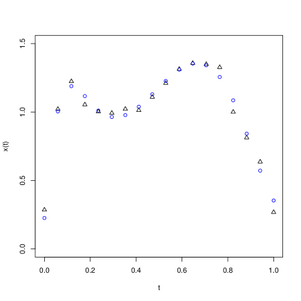
This application of Subsection 4.2 takes $K=8$ spline functions of order $m=5$ (and are constructed using the R package splines with knot sequence $(0,0,0,0,0,0.25,0.5,0.75,1,1,1,1,1)$ and option monoH.FC). Figure 2 plots the resulting set of spline functions $\{B_{k,5}(t)\}_{k=1}^{8}$ over $t\in[0,1]$. As described in Subsection 4.2, each of the 3,158 discretized curves $\bm{x}$ can be approximated by a spline $\sum_{k=1}^{8}\widehat{\alpha}^{(i)}_{k}B_{k,5}(t)$. This representation results in a dimension reduction from $18$ to $8$, and provides a good fit of the 3,158 curves. Figure 5 plots the original and spline approximation for the curve $\bm{x}_{i}$ having largest mean square difference from its spline approximation, among the 3,158 historical curves.

Figure 5: Original (black triangles) and spline approximation (blue circles) for the curve $\bm{x}_{i}=(x_{i,1},\ldots,x_{i,18})$ having the largest mean square difference compared with its spline approximation, among the 3,158 historical curves.

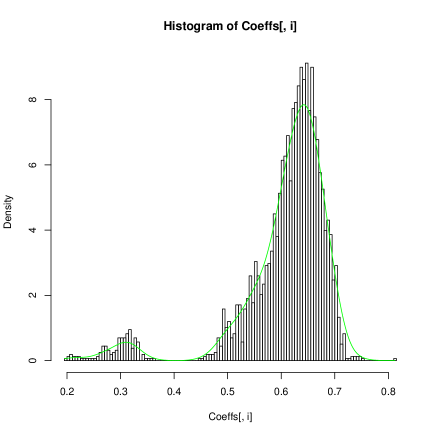
Kernel density estimation is performed as described in Subsection 2. The window vector obtained is $(\widehat{\lambda}_{1},\ldots,\widehat{\lambda}_{8})\approx(0.018,0.019,0.019,0.018,0.017,0.015,0.021,0.017)$. To illustrate, Figure 6 plots the density of the first marginal probability density function of the ($8$-dimensional) probability density function $\rho_{\widehat{\lambda}_{1},\ldots,\widehat{\lambda}_{8}}$ together with the histogram of $\widehat{\alpha}^{(1)}_{1},\ldots,\widehat{\alpha}^{(3,158)}_{1}$.

Figure 6: Plot of the first marginal probability density function of the ($8$-d) probability density function $\rho_{\widehat{\lambda}_{1},\ldots,\widehat{\lambda}_{8}}$ (in green), together with the histogram of the first components $\widehat{\alpha}^{(1)}_{1},\ldots,\widehat{\alpha}^{(3,158)}_{1}$ from the spline kernel basis representations of the 3,158 curves.

The threshold value is selected as described in Subsection 2, where $\Delta=0.05$ is chosen, and is $\widehat{T}=54.86$. Figure 7 provides a visual insight of the domain $\{\bm{\alpha}$ $:$ $\widehat{\rho}(\bm{\alpha})\geq\widehat{T}\}$. Coefficient vectors $\widehat{\bm{\alpha}}^{(i_{1})}$ and $\widehat{\bm{\alpha}}^{(i_{2})}$ are considered for two of the historical inputs, where $\widehat{\bm{\alpha}}^{(i_{1})}$ is numerically distant from the remaining $\{\widehat{\bm{\alpha}}^{(i)}\}_{i\neq i_{1}}$, while $\widehat{\bm{\alpha}}^{(i_{2})}$ has closer neighbors. As a consequence $\widehat{\rho}(\widehat{\bm{\alpha}}^{(i_{2})})>\widehat{\rho}(\widehat{\bm{\alpha}}^{(i_{1})})$. The value of $\widehat{\rho}(\bm{\alpha})$ is plotted, for $\bm{\alpha}$ belonging to the segment with endpoints $\widehat{\bm{\alpha}}^{(i_{1})}-0.1\left(\widehat{\bm{\alpha}}^{(i_{2})}-\widehat{\bm{\alpha}}^{(i_{1})}\right)$ and $\widehat{\bm{\alpha}}^{(i_{1})}+1.1\left(\widehat{\bm{\alpha}}^{(i_{2})}-\widehat{\bm{\alpha}}^{(i_{1})}\right)$. One observes that the parts of the segment close to ${\widehat{\bm{\alpha}}^{(i_{1})}}$ and ${\widehat{\bm{\alpha}}^{(i_{2})}}$ correspond to admissible $\bm{\alpha}$’s, while the middle of the segment corresponds to inadmissible $\bm{\alpha}$’s. Recall that $\Delta$ is user selected and that decreasing it increases the threshold and vice versa.

Figure 7: Values of $\log(1+\widehat{\rho}({\bm{\alpha}}))$ (black dots), for $\bm{\alpha}$ belonging to the segment with endpoints obtained from a isolated historical coefficient vector and a non-isolated one. The red line is the logarithm of (1 plus the threshold).

5.3 Optimization of an Analytical Function

This subsection maximizes an analytical function $y(\bm{x})$ over the domain of the simplex determined from the $n=$ $3$,$158$ historical curves from the nuclear power industry. Both the expert-type constraints methodology and the kernel density approximation will be illustrated to identify this input space. The analytical function to be maximized is

$$y_{a}(\bm{x})=-||\bm{x}-\bm{x}_{0}||_{2}-\sin\left(3||\bm{x}-\bm{x}_{0}||_{2}\right)^{2},$$ (17)

where $\bm{x}_{0}$ is a fixed one of the $n=$ 3,158 historical curves and $||\bm{w}||_{2}=(\bm{w}^{\top}\bm{w})^{1/2}$ for a column vector $\bm{w}$. The unique maximizer of $y_{a}(\bm{x})$ in (4) is $\bm{x}=\bm{x}_{0}$ with optimal value $y_{a}(\bm{x}_{0})=0$. The function $y_{a}(\bm{x})$ is observed with additive Gaussian noise having mean zero and variance $0.0005^{2}$. This mild Monte Carlo noise in the $y(\bm{x})$ function mimics that present in the second example.

The goal is to assess whether the expected improvement algorithm is able to converge to the global maximizer for both the expert-type constraint domain in (4) or the domain defined using kernel density approximation in (16).

EI Optimization of (17) over ${\cal X}$ Determined by Expert-Type Constraints

The set of training curves used for the analytic function consisted of $100$ curves selected by a space-filling design among the 3,158 historical input vectors. The maximum value of $y_{a}(\bm{x})$ among the training data is approximately $-0.75$. Then $50$ additional discretized curves were selected from ${\cal X}$ using the EI/expert knowledge procedure. The maximum $y_{a}(\bm{x})$ increased to approximately $-0.17$ using the $50$ additional curves.

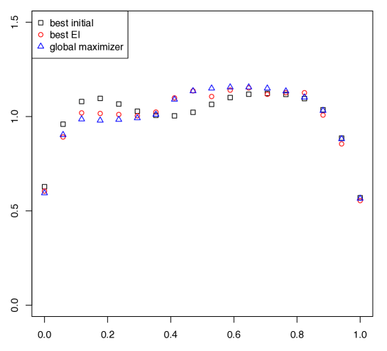
Figure 8 provides a visual understanding of this performance by plotting three curves that illustrate the performance of the proposed procedure. The first curve is $\bm{x}_{0}$ which denotes the true global maximizer; the second curve, denoted $\bm{x}_{\mathrm{init}}$, is the maximizer of $y_{a}(\bm{x})$ among the $100$ initial curves; the third curve, denoted $\bm{x}_{\mathrm{EI}}$, is the maximizer of $y_{a}(\bm{x})$ among the $50$ curves obtained by expected improvement. Observe that $\bm{x}_{\mathrm{EI}}$ is, visually, significantly closer to $\bm{x}_{0}$ than is $\bm{x}_{\mathrm{init}}$, which suggests the convergence of the expected improvement procedure. This example also shows that the admissible set in (4) is amenable to maximization in practice.

Figure 8: Three input curves for the analytic optimization problem (17): the true global $y_{a}(\bm{x})$ maximizer; the $y_{a}(\bm{x})$ maximizer among the $100$ initial curves; the $y_{a}(\bm{x})$ maximizer among the $50$ curves added by EI/expert-type constraints based on (5)-(8).

EI Optimization of (17) over ${\cal X}$ Determined by Kernel Density Estimation

In this case, while the analytical function $y_{a}(\bm{x})$ is (17), the curve $\bm{x}_{0}$ is now given by $(x_{0}(t_{1}),\ldots,x_{0}(t_{d}))$, with

$$x_{0}(t)=\frac{\sum_{i=1}^{K}\alpha_{0,i}B_{i,m}(t)}{\frac{1}{d}\sum_{j=1}^{d}\sum_{i=1}^{K}\alpha_{0,i}B_{i,m}(t_{j})}$$

where $\bm{\alpha}_{0}$ is one of the $3$,$158$ $\widehat{\bm{\alpha}}^{(1)},\ldots,\widehat{\bm{\alpha}}^{(3158)}$. Thus in the optimization problem (16), the global maximizer curve is given by $\bm{\alpha}^{\star}=\bm{\alpha}_{0}$. Noisy observations of $y_{a}(\bm{x})$ are obtained as above.

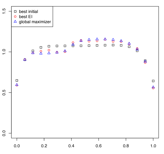
The initial random design of $100$ curves was obtained similarly to that for the expert knowledge procedure above; the sequentially added $50$ curves were obtained by the EI/kernel density estimation procedure. The conclusions are similar to those for the EI/expert knowledge procedure. Namely, among the initial $100$ training data curves, the maximum value of $y_{a}(\bm{x})$ is approximately $-0.71$ which occurs at $\bm{x}_{\mathrm{init}}$. With the $50$ additional curves obtained by expected improvement, this maximum increases to approximately $-0.11$ at $\bm{x}_{\mathrm{EI}}$. Figure 9 plots the three curves $\bm{x}_{\mathrm{init}}$, $\bm{x}_{\mathrm{EI}}$ and $\bm{x}_{0}$.

Figure 9: Three input curves for the analytic optimization problem (17): the true global $y_{a}(\bm{x})$ maximizer; the $y_{a}(\bm{x})$ maximizer among the $100$ initial curves; the $y_{a}(\bm{x})$ maximizer among the $50$ curves added by EI/kernel density estimation.

5.4 Optimizing Burn-up Credit Penalization

In this subsection the expected improvement procedure is carried out similarly as in Subsection 5.3 with the analytical function $y_{a}(\bm{x})$ replaced by CRISTAL code function $y(\bm{x})$ evaluations.

For both methods of identifying the valid input space, ${\cal{X}}$, the EI algorithm was carried out starting from a Gaussian Process model based on $100$ observed values of $y(\bm{x})$. For EI/kernel density via the optimization problem (16), these observed values corresponded to a subset $\{\widehat{\bm{\alpha}}^{(i_{1})},\ldots,\widehat{\bm{\alpha}}^{(i_{100})}\}$ of $\{\widehat{\bm{\alpha}}^{(1)},\ldots,\widehat{\bm{\alpha}}^{(3,158)}\}$. This subset was selected by the following space-filling procedure. First, $100$ barycenters where computed from a K means clustering algorithm applied to $\{\widehat{\bm{\alpha}}^{(1)},\ldots,\widehat{\bm{\alpha}}^{(3,158)}\}$. Then, the $\{\widehat{\bm{\alpha}}^{(i_{1})},\ldots,\widehat{\bm{\alpha}}^{(i_{100})}\}$ closest to these barycenters were selected. The CRISTAL code was run $100$ times to compute the corresponding $y(\bm{x}(\widehat{\bm{\alpha}}^{(i_{1})})/\bar{\bm{x}}(\widehat{\bm{\alpha}}^{(i_{1})}))$ , …, $y(\bm{x}(\widehat{\bm{\alpha}}^{(i_{100})})/\bar{\bm{x}}(\widehat{\bm{\alpha}}^{(i_{100})}))$.

For the EI/expert constraints method, a subset $\{\bm{x}_{i_{1}},\ldots,\bm{x}_{i_{100}}\}$ of $\{\bm{x}_{1},\ldots,\bm{x}_{3,158}\}$ was obtained, using the same space-filling procedure as above. The corresponding $y(\bm{x}_{i_{1}}),\ldots,y(\bm{x}_{i_{100}})$ were selected from the historical data base.

The number of initial values for expected improvement, $100$, was hence selected for two reasons. First reason is that 100 initial observations allows an interpretable comparison between the results of EI using expert knowledge versus kernel density estimation methods. The second reason was based on computational budget considerations. In the future, the Burn-up Credit code is expected to become more complex and costly to evaluate. It was extrapolated that the value $100$ satisfies future budget constraints and suggests the performance of the two input determination methods.

EI optimization of Burn-up Credit Penalization

Figure 10: The cumulative maxima, $\max\left\{m_{\mathrm{hist}},y(\bm{x}_{EI,1}),\ldots,y(\bm{x}_{EI,i})\right\}$, as a function of the iteration index $i$ for EI based on the expert-type constraints (left panel) and on kernel density estimation (right panel). The symbol $m_{\mathrm{hist}}$ denotes the maximum value of $y(\bm{x})$ among the $100$ training data input curves.

The maximum of $\{y(\bm{x}_{1}),\ldots,y(\bm{x}_{3,158})\}$ is equal to $0.94123$. This illustrates the maximization performance using only the historical data base (although these values contain a small Monte Carlo noise). Starting with 100 training inputs and their corresponding $y(\bm{x})$ values and then running $100$ iterations of the expected improvement procedure yields new curves $\bm{x}_{EI,1},\ldots,\bm{x}_{EI,100}$ for both the EI/expert constraints and EI/kernel density estimation procedures. The maximum of $y(\bm{x}_{EI,1}),\ldots,y(\bm{x}_{EI,100})$ is $0.95535$ for the EI/expert constraints procedure and is $0.94761$ for the EI/kernel density estimation procedure. Hence, the admissible set obtained from the expert knowledge is larger, so to speak, than that obtained from the kernel density estimation procedure, and allows for larger values of $y(\bm{x})$. This is possibly due to the choices of the tolerance values $\epsilon$ and of the distance $\Delta$ (see Section 4). One may also notice that, in essence, the EI/expert constraints procedure allows for a larger search space for optimization, as it does not project the curves onto a lower dimensional space.

To show the effectiveness of the two EI procedures, Figure 10 plots the cumulative maxima of $y(\bm{x})$, including that based on the training data, for the $100$ EI iterations. The convergence appears to be relatively fast when ${\cal X}$ is determined by expert constraints. When ${\cal X}$ is determined by kernel density estimation, additional iterations of expected improvement would likely result in a further improvement of $y(\bm{x})$.

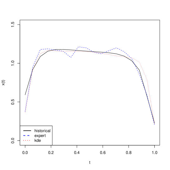
Finally Figure 11 plots the three curves $\bm{x}_{\mathrm{hist}}$, $\bm{x}_{\mathrm{expert}}$, and $\bm{x}_{\mathrm{kde}}$, where $\bm{x}_{\mathrm{hist}}$ corresponds to the maximum of the historical values $\{y(\bm{x}_{1}),\ldots,y(\bm{x}_{3,158})\}$ and $\bm{x}_{\mathrm{expert}}$ (resp. $\bm{x}_{\mathrm{kde}}$) corresponds to the maximum of $y(\bm{x}_{EI,1}),\ldots,y(\bm{x}_{EI,100})$ for the EI/expert constraints (resp. EI/ kernel density estimation) procedure. The deviation from $\bm{x}_{\mathrm{expert}}$ and $\bm{x}_{\mathrm{kde}}$ to $\bm{x}_{\mathrm{hist}}$ is moderate but non-negligible. We also observe that $\bm{x}_{\mathrm{kde}}$ is smoother than $\bm{x}_{\mathrm{expert}}$, which is a feature of the spline decomposition.

Figure 11: Curves that maximize the Burn-up Credit Penalization: (1) among the 3,158 historical curves; (2) among the 100 curves added by the EI/expert constraints procedure; (3) among the 100 curves added by the EI/kernel density estimation procedure.

5.5 Breath of Application of the Method and an Illustrative Example

Although the present methodology has been presented together with the motivating fuel rod application case, its level of generality goes beyond this case. Indeed, the methodology can be applied to any setting where the two following features are present. (1) There is an unknown function domain

$$\mathcal{F}\subset\left\{\bm{x}:[0,1]\to\mathbb{R}\right\},$$

where the domain of the functions is conventionally fixed to $[0,1]$, without loss of generality. The corresponding set of discretized curves is

$$\mathcal{F}_{d}=\left\{\bm{x}=(x(t_{1}),\ldots,x(t_{d}))^{\top};x\in\mathcal{F}\right\},$$

for fixed grid knots $0\leq t_{1}<\dots<t_{d}\leq 1$. Discretized functions $\bm{x}_{1},\ldots,\bm{x}_{n}\in\mathcal{F}_{d}$ are available. (2) There is a simulator $y:\mathcal{F}_{d}\to\mathbb{R}$, where $y(\bm{x})$ can be evaluated (with or without noise) for any $\bm{x}\in\mathbb{R}^{d}$ (or any $\bm{x}$ in a fixed known subset of $\mathbb{R}^{d}$ containing $\mathcal{F}_{d}$). Each evaluation of $y(\bm{x})$ is costly and thus the total number of evaluations is limited.

The objective is to solve the constrained optimization problem

$$\max_{\bm{x}\in\mathcal{F}_{d}}y(\bm{x}),$$ (18)

that is to simultaneously estimate the unknown $\mathcal{F}_{d}$ from the historical $\bm{x}_{1},\ldots,\bm{x}_{n}$ and optimize $y$. The fuel rod application introduced in Section 2 and addressed in Subsection 5.4 is thus a special case of this general framework.

The methodology introduced here (that is the two methods for determining the input domain in Section 4 followed by the EI procedure) can be readily applied to the general problem (18). Note that the methodology is not restricted to the constraint of positive-valued elements in $\mathcal{F}_{d}$ averaging to $1$, as in the fuel rod application. Indeed, if this constraint is not present, one may just omit all the normalization steps (dividing a vector by its average).

Let us now provide an application of the methodology to an analytical test case. Consider the grid knots $t_{1}=0,t_{2}=1/20,\ldots,t_{d}=1$ with $d=21$. Consider the function domain

$$\mathcal{F}=\left\{\bm{x}_{a,b,c};(a,b,c)\in[4,12]\times[2,5]\times[0.8,1.2]\right\},$$ (19)

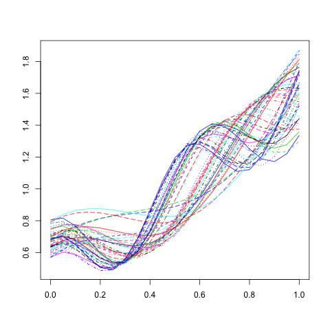
with $x_{a,b,c}(t)=(1+\cos(at)+bt+\exp(ct))/C_{a,b,c}$ where $C_{a,b,c}=(1/d)\sum_{i=1}^{d}(1+\cos(at_{i})+bt_{i}+\exp(ct_{i}))$. Hence, $\mathcal{F}_{d}$ is composed of vectors averaging to $1$. We consider an historical data set of size $n=1,000$ obtained by independent random sampling of elements in $\mathcal{F}_{d}$ by sampling $(a,b,c)$ uniformly on $[4,12]\times[2,5]\times[0.8,1.2]$. Figure 12 shows $50$ of these discretized functions.

Figure 12: Fifty historical curves for the analytical example of Subsection 5.5.

We consider the curve $\bm{x}_{12,6,1}$ (slightly outside $\mathcal{F}$) and its discretized version $\bm{x}_{12,6,1}$ (slightly outside $\mathcal{F}_{d}$). Then the code function is defined as, for any $\bm{x}=(x_{1},\ldots,x_{d})^{\top}$,

$$y(\bm{x})=-\left|\left|\bm{x}-\bm{x}_{12,6,1}\right|\right|_{2}-\sin\left(3\left|\left|\bm{x}-\bm{x}_{12,6,1}\right|\right|_{2}\right)^{2}.$$

The theoretical maximizer of (18) is thus close to $\bm{x}_{12,6,1}$. The global maximum and maximizer of (18) are computed by a brute force method with $10^{6}$ evaluations of $y$. The maximum is approximately $-0.08$.

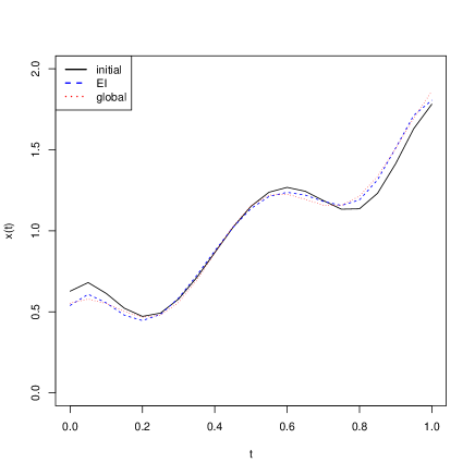
We first carry out the methodology based on projections onto a basis set followed by optimization by EI (Subsection 4.2). Here there is no noise in the evaluations of $y$ nor in the Gaussian process model of EI. Otherwise, we use the same settings as for the fuel rod application (Subsections 5.2 and 5.4), in particular the same spline basis functions and the same value $\Delta=0.05$ in (13). For optimization, we select $30$ curves based on the same space filling construction as in Subsection 5.4. We then run $30$ iterations of the EI procedure. The maximum of the values of $y$ over the $30$ initial curves is approximately $-0.84$. The maximum of the values of $y$ after the $30$ EI iterations is approximately $-0.20$. Figure 13 shows the cumulative maxima of the values of $y$ along the EI iterations and the best of the $30$ initial curves, the curve found by EI and the global maximizer curve. The conclusion is that the methodology is successful here. With only $60$ calls to the code function, it yields a value of $y$ which is close to the maximum in (18), and a corresponding curve which is visually very close to the maximizer in (18). Furthermore, the curve obtained by EI is significantly closer to the global maximizer than the curve obtained by the initial space filling design. Finally, we remark that the employed methodology needs no knowledge of the nature of the set (19), which is completely unrelated to the spline basis functions used.

Figure 13: Analytical example of Subsection 5.5 for the methodology based on projections onto a basis set followed by optimization by EI. Left: cumulative maxima of $y$ values along EI iterations. Right: best of the $30$ initial curves, the curve found by EI and the global maximizer curve.

Second, we carry out the methodology based on expert-type constraints followed by optimization by EI (Subsection 4.1). Again, there is no noise in the evaluations of $y$ nor in the Gaussian process model of EI and, otherwise, we use the same settings as for the fuel rod application (Subsections 5.2 and 5.4), in particular the same list of constraints and tolerance levels $\epsilon$. Remark that the constraints related to the time steps $16,17,18$ for the fuel rod application naturally correspond to constraints related to the time steps $19,20,21$ here. Again, for the optimization, we select $30$ curves based on the same space filling construction as in Subsection 5.4 and we run $30$ iterations of the EI procedure. The maximum of the values of $y$ over the $30$ initial curves is approximately $-0.89$. The maximum of the values of $y$ after the $30$ EI iterations is approximately $-0.48$. Figure 14 is then similar to Figure 13. The conclusion that the methodology is successful also holds, similarly as previously. Compared to the methodology based on projections onto a basis set, we remark that the convergence of EI is slightly slower and that the curve found by EI is more irregular. This irregularity is similarly observed in Figure 11 for the fuel rod application, and holds because the expert knowledge methodology does not project the curves onto function spaces, but instead treats them as $d$-dimensional vectors.

Figure 14: Analytical example of Subsection 5.5 for the methodology based on expert-type constraints followed by optimization by EI. Left: cumulative maxima of $y$ values along EI iterations. Right: best of the $30$ initial curves, the curve found by EI and the global maximizer curve.

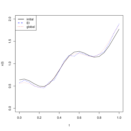In summary, Figures 13 and 14 illustrate the robustness of the present suggested methodology. Indeed, the methodology, as calibrated for the fuel rod application (in particular the choice of the spline projection functions, of the expert-type constraints and of various numerical parameters), proves to be efficient in the new setting (18). Of course, in other specific settings, other choices of calibration (for instance other expert-type constraints) may lead to even better results.

Let us conclude Subsection 5.5, by further discussing the generality of the present framework and methodology. In (18), we have presented a general framework where optimization over an unknown domain of one-dimensional curves is considered. In the fuel rod application, these one-dimensional curves correspond to spatial dependence, since they provide the spatial distribution of the burn-up rate.

In (18), the $d$ grid knots are the same for all the curves, which is the case for the fuel rod application motivating the present work. While the case of identical grid knots among the historical curves is relatively common, it may happen that each curve is discretized on a different set of knots. In this case, as mentioned in Section 2, various interpolation schemes can be applied. If each curve is discretized at a large number of knots, then function approximation principles suggest that the impact of the interpolation scheme will be small. If some curves are discretized at a small number of knots, then the choice of the interpolation scheme may influence the final results. Studying this influence in further real examples deserves to be the topic of future work.

The framework and methodology could be extended to optimizing over an unknown domain of two-dimensional surfaces (typically if a temporal dependence is also tackled) or higher dimensional functions. Indeed, one may still define constraints as in Subsection 4.1, for instance using finite differences in various directions, or extending the notion of total variation to the multi-dimensional case. Similarly, as in Subsection 4.2, one may decompose the surfaces or functions on finite-dimensional bases of multi-dimensional functions.

When considering an unknown domain of multi-dimensional surfaces, the optimization space becomes more complex, and applying EI can become more challenging. Specific procedures for high-dimensional optimization based on EI, for instance Ben Salem et al. (2019), may be relevant in this case. Depending on the physical application, other aspects may be present and yield further complexity and multi-dimensional heterogeneity. While the current results indicate that our suggested methodology can be applicable in the various more complex settings discussed above (as it is robust as discussed above), in future work, it would be valuable to further test it in these settings.

6 Summary and Discussion

This paper proposes methods to identify a potentially complicated input optimization domain which is known to be a subset of the simplex, based on observational historical data that are known to belong to the input domain. It also shows how a variant of the EGO algorithm for deterministic output can be applied to optimize the mean output of a stochastic simulator over this domain. The expected improvement function is maximized over an input region of positive Lebesgue measure by applying a linear transformation of the simplex to a lower-dimensional space.

The application of these methods to a large validated historical database of burn-up profiles is an original proposal to solve the problem of burn-up credit in nuclear safety assessment. It has to be compared with current approaches, such as ones that use pre-defined profiles to check the sub-criticality of burned assemblies. More broadly, in applications where it tends to be difficult to pre-define reference profiles (like in mixed oxides fuels), a more general approach like the one presented here should be more robust.

We conclude by mentioning two problems that have not been addressed in this paper but are topics for future research. The first problem stems from the frequently-occurring need in climate science and other scientific areas to build adaptively an input domain from training data. Climate models consist of submodels for surface temperatures, wind magnitude, wind velocity, sea surface temperatures and other interacting constituents that determine the climate. These submodels must all be computable and verifiable. The bounds on the input domain where all the composite models can be simultaneously run is unknown and can be complex. Thus the problem of identifying the input region is one of sequential design. A series of inputs is identified with the resulting attempted model run being successful or not. These data are used to estimate the input domain. The second problem is the determination of sensitivity analysis tools for the mean of a stochastic simulator when the input domain is an estimated subset of the simplex. The research of Loeppky et al. (2013) who developed global sensitivity tools for deterministic simulator output defined on the simplex is a starting point for this more complicated scenario.

ACKNOWLEDGMENTS

The authors wish to thank two anonymous referees, for suggestions which led to an improvement of this paper.

This research was conducted with the support of the Chair in Applied Mathematics OQUAIDO, gathering partners in technological research (BRGM, CEA, IFPEN, IRSN, Safran, Storengy) and academia (CNRS, Ecole Centrale de Lyon, Mines Saint-Étienne, University of Grenoble, University of Nice, University of Toulouse) in the development of advanced methods for Computer Experiments.

The authors would like also to thank the Isaac Newton Institute for Mathematical Sciences for support and hospitality during the programme on Uncertainty Quantification when work on this paper was undertaken and The Statistical and Applied Mathematical Sciences Institute for support and hospitality during the program Model Uncertainty: Mathematical and Statistical. Finally, this work was supported by: EPSRC grant numbers EP/K032208/1 and EP/R014604/1. This research was also sponsored, in part, by the National Science Foundation under Agreements DMS-0806134 and DMS-1310294 (The Ohio State University). Any opinions, findings, and conclusions or recommendations expressed in this material are those of the authors and do not necessarily reflect the views of the National Science Foundation.

References

- Ben Salem et al. (2019) M. Ben Salem, F. Bachoc, O. Roustant, F. Gamboa and L. Tomaso. Gaussian process-based dimension reduction for goal-oriented sequential design. SIAM/ASA Journal on Uncertainty Quantification, 7(4):1369–1397, 2019.
- Cacciapouti and Volkinburg (1997) R. J. Cacciapouti and S. Van Volkinburg. Axial burnup profile database for pressurized water reactors. Technical Report USCD1219 ZZ-PWR-AXBUPRO-SNL, OECD Nuclear Energy Agency Data Bank, 1997.
- Cacuci (2010) D. G. Cacuci. Handbook of Nuclear Engineering: Vol. 1: Nuclear Engineering Fundamentals; Vol. 2: Reactor Design; Vol. 3: Reactor Analysis; Vol. 4: Reactors of Generations III and IV; Vol. 5: Fuel Cycles, Decommissioning, Waste Disposal and Safeguards, volume 2. Springer Science & Business Media, 2010.
- CRISTAL (2018) CRISTAL. Criticality Calculation Package, v2.0.2,. OECD Nuclear Energy Agency Data Bank, NEA-1903, 2018. URL http://www.cristal-package.org.
- de Klerk (2008) E. de Klerk. The complexity of optimizing over a simplex, hypercube or sphere: A short survey. Central European Journal of Operations Research, 16(2):111–125, 2008.
- Draguljić et al. (2012) D. Draguljić, T. J. Santner, and A. M. Dean. Non-collapsing spacing-filling designs for bounded polygonal regions. Technometrics, 54:169–178, 2012.
- Jones et al. (1998) D. R. Jones, M. Schonlau, and W. J. Welch. Efficient global optimization of expensive black–box functions. Journal of Global Optimization, 13:455–492, 1998.
- Loeppky et al. (2013) J. L. Loeppky, B. J. Williams, and L. M. Moore. Global sensitivity analysis for mixture experiments. Technometrics, 55:68–78, 2013.
- Muehlenstaedt et al. (2017) T. Muehlenstaedt, J. Fruth, and O. Roustant. Computer experiments with functional inputs and scalar outputs by a norm-based approach. Statistics and Computing, 27(4):1083–1097, 2017.
- Perrin et al. (2018) G. Perrin, C. Soize, and N. Ouhbi. Data-driven kernel representations for sampling with an unknown block dependence structure under correlation constraints. Computational Statistics & Data Analysis, 119:139–154, 2018.
- Picheny et al. (2013) V. Picheny, D. Ginsbourger, Y. Richet, and G. Caplin. Quantile-based optimization of noisy computer experiments with tunable precision. Technometrics, 55(1):2–13, 2013.
- Ramsay (2006) J. O Ramsay. Functional data analysis. Wiley Online Library, 2006.
- Santner et al. (2018) T. J. Santner, B. J. Willams, and W. I. Notz. The Design and Analysis of Computer Experiments, Second Edition. Springer Verlag, New York, 2018.
- Schonlau et al. (1998) M. Schonlau, W. J. Welch, and D. R. Jones. Global versus local search in constrained optimization of computer models. In N. Flournoy, W. F. Rosenberger, and W. K. Wong, editors, New Developments and Applications in Experimental Design, volume 34, pages 11–25. Institute of Mathematical Statistics, 1998.
- Stinstra et al. (2003) E. Stinstra, D. den Hertog, P. Stehouwer, and A. Vestjens. Constrained maximin designs for computer experiments. Technometrics, 45(4):340–346, 2003.