reaction for particles with a dynamic bias to move away from their nearest neighbour in one dimension
Abstract
We consider the dynamics of particles undergoing the reaction in one dimension with a dynamic bias. Here the particles move towards their nearest neighbour with probability where . is the deterministic limit where the nearest neighbour interaction is strictly repulsive. We show that the negative bias changes drastically the behaviour of the fraction of surviving particles and persistence probability with time . decays as where increases with . shows a stretched exponential decay with non-universal decay parameters. The probability that a tagged particle is at position from its origin is found to be Gaussian for all ; the associated scaling variable is where approaches the known limiting value as , in a power law manner. Some additional features of the dynamics by tagging the particles are also studied. The results are compared to the case of positive bias, a well studied problem.
1 Introduction
Reaction diffusion systems have been extensively studied over the last few decades, especially in one dimension [1, 2, 3, 4, 5, 6, 7, 8, 9, 10, 11, 12, 13]. The simplest form of a reaction diffusion system is , where the particles diffuse and annihilate on contact. This model in one dimension, with asynchronous updating, also represents the ordering dynamics of the Ising model with Glauber dynamics at zero temperature. When considered on a lattice, one can assume that the particles occupy the sites of the lattice and at each time step they hop to a nearest neighbouring site.
The system has been studied in the recent past where the particles move with a bias towards their nearest neighbours [14, 15, 16] in one dimension. The model, in its deterministic limit, maps to a opinion dynamics model studied earlier [17]. Previously, both the bulk dynamical and tagged particle dynamics have been reported in the one dimensional system where the particle diffuses towards its nearest neighbour with a probability and in the opposite direction with probability . The results show significant differences when compared to the case with no bias () although the annihilation process is identical in the latter. This reaction diffusion model with parallel updating has also been studied in two dimensions recently [18].
To generalize the problem, in the present paper, the results for a negative bias are reported, i.e., when . The idea behind the study is to find the universal behaviour in the bulk properties as well as the microscopic features. Here we have used asynchronous dynamics to compare with the positive bias case results which have already been studied before. Specifically, implies purely repulsive motion where the particles always move towards their farther neighbour. These particles with full negative bias can represent the motion of similarly charged particles or in general particles with repulsive interaction which can move both ways. Henceforth we denote the fully biased point by .
2 The Model, dynamics and simulation details

In the model, a particle diffuses to one of its neighbouring sites and undergoes a reaction (annihilation). Here, at each update, a site is randomly chosen and if there is a particle on the selected site, it hops one step towards its nearest neighbour with probability (and with probability in the opposite direction); . If the destination site is previously occupied by a particle, both of them will be annihilated simultaneously. The position of the particle is updated immediately in the asynchronous scheme of updating. such updates constitute one Monte Carlo step (MCS). In the rare cases of two equidistant neighbours, the particle moves in either direction with equal probability 0.5. The motion is illustrated in figure 1. It may be noted that the direction of motion is determined by the relative distances of the neighbouring particles only; the particle has a tendency to move away from the nearest neighbour (for , which is the choice here). The actual distances are of no consideration in the present scenario. Also, if a site is chosen for updating, the particle sitting at that site has to perform a move.
As asynchronous dynamics have been used, there are several interesting points to be noted. The net displacement of a particle can be zero or more than one after the completion of one MCS [16]. This affects the numerical estimates of certain quantities that have been estimated in the present work. For the fully biased point , annihilation can occur only if three particles occupy immediately adjacent sites, however, in the asynchronous update scheme, whether an annihilation will take place will depend on which site is getting updated first, so it is a necessary but not sufficient condition.
The studies are performed on lattices of maximum size and the maximum number of initial configurations taken is 2000. Periodic boundary condition has been used in all the simulations. We have considered the lattice of size to be randomly half filled initially.
3 Simulation Results
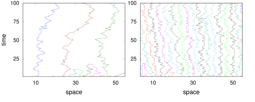
We took snapshots of the system to check the motion of individual particles. The world lines of the motion of the particles are shown for and in figure 2. It may be noted immediately they are strikingly different from each other. It is obvious that the number of annihilation is larger for and it is left with much fewer particles within the same timescale. Also, the paths traced out resemble more a diffusive trajectory. In contrast, for , the particles change their direction more often and remain confined within a limited region in space.
To probe the dynamics of the particles, we have studied the following quantities: (i) fraction of surviving particles at time , (ii) persistence probability of the lattice sites , (iii) the probability distribution of finding a particle at distance from its origin at time , (iv) the probability of the change in the direction in the motion of a particle at time and (v) the distribution of the time interval between two successive changes in the direction of the motion of a particle. The results for each of these quantities are presented in the following subsections.
3.1 Bulk properties
3.1.1 Fraction of surviving particles
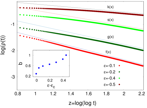
For the purely diffusive system (), it is well known that the fraction of surviving particles shows a power law behaviour in time; with . If a positive bias in introduced in the system, for all [14, 15]. The exponent increases as the attractive dynamics result in an increased number of annihilation. As is made negative, the number of annihilation decreases as reaction becomes less probable because of the repulsion. So, shows a slow decay in time and can be fitted to the following form
| (1) |
where and are constants, depending on . The fitting is made with a two parameter least square fitting using GNUFIT. In figure 3, is plotted against for different values, to manifest the linear dependence at long times. Here it may be mentioned that for the extreme point , the particles ideally attain a equidistant configuration. But the dynamical rule is such that the particles have to make a move and hence they perform a nearly oscillatory motion. Annihilation takes place extremely rarely at large times such that decreases as the magnitude of increases (see inset of figure 3).
3.1.2 Persistence probability
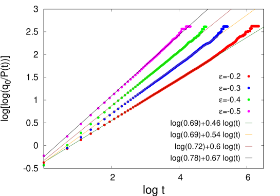
Persistence probability in this model is defined as the probability that a site is unvisited till time . For , decays as with [19]. For , , however small be the bias [14]. As becomes negative, falls off rapidly (see figure 4). shows a stretched exponential decay in time:
| (2) |
Once again, the best fit curves with a three parameter function are obtained using GNUFIT. In figure 4 we show the validity of the above form by obtaining linear dependence when is plotted against . Both and increase as .
3.2 Tagged particle features
3.2.1 Probability distribution
For pure random walk (), the probability distribution is known to be Gaussian and shows a data collapse for different times when plotted against . This is also true for the unbiased () annihilating random walkers because they perform purely diffusive motion until they are annihilated. For , the distributions can again be fit to a Gaussian form. However the scaling variable is in general with . We extract the value of from the data using two different methods.
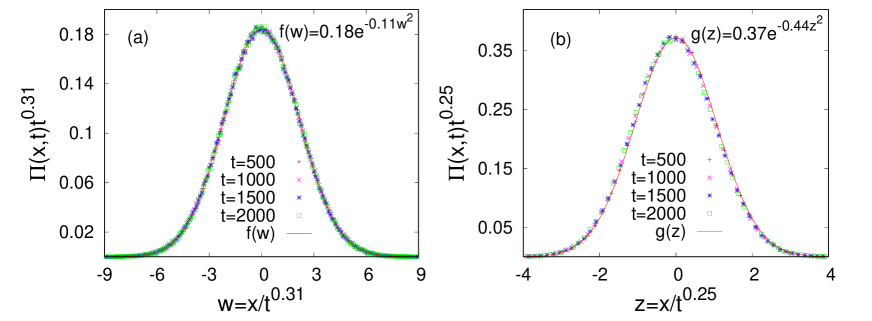
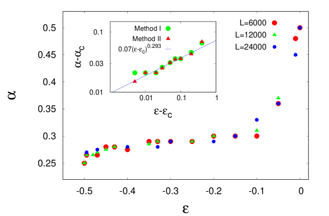
Method I: In this method the scaling variable is obtained by collapsing the data using trial values of and choosing the value for which the data collapse looks most impressive (see figure 5). This analysis indicates that depends on , the values are shown in figure 6. There seems to be some finite size dependence which, however, could not be systematically captured in this method. As decreases from zero, at first decays rapidly from the value 0.5 at until where it attains a value close to 0.3. Below , shows a slow decrease and at , it is close to 0.25, the value expected for repulsive random walkers [20]. At large time as the walkers do not annihilate, effectively they perform repulsive random walk in the lattice. The typical error involved in the above estimates is .
Method II: The values of obtained from Method I indicates that has a comparatively weaker variation with for . To obtain a more accurate dependence of for , we employ another method that optimises the value of needed to obtain the best data collapse. Here we utilise the fact that the scaling function is Gaussian. Method II is based on the prescription given in [21], when the form of the scaling function is known.
For a given value, we use the same four sets of data corresponding to four different times that were used to get the collapse in Method I. We first choose a value of and taking any of the four sets of data (say, the th set with a probability distribution ), fit a Gaussian function to the scaled probability distribution . The scaling variable here is such that
| (3) |
Knowing and from the fitting, we now choose another set , and estimate the deviation from the above Gaussian function by calculating
| (4) |
denotes average over all the discrete points in the th data set. The total averaged error for the choice of the th set as the initial set is then equal to .
Next we repeat the above exercise by choosing a different set as the initial set to get and finally compute the averaged error
| (5) |
Plotting against , a minimum value is expected at a certain value of which is identified as the optimal value that gives the best data collapse.
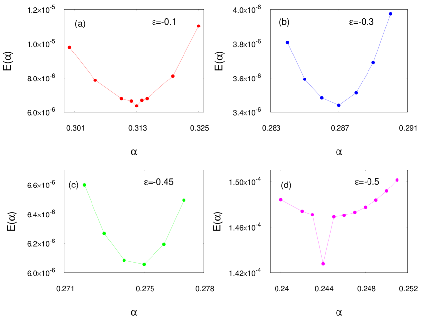
A minimum value of ) is indeed obtained as we vary the value of in steps of 0.001. The results for are shown for different vales of in figure 7. The values of where corresponds to are plotted in the inset of figure 6 obtained from both the methods and a log-log plot shows that a variation
| (6) |
is quite compatible with the more accurate estimates of Method II close to small values of .
3.2.2 Probability of direction change
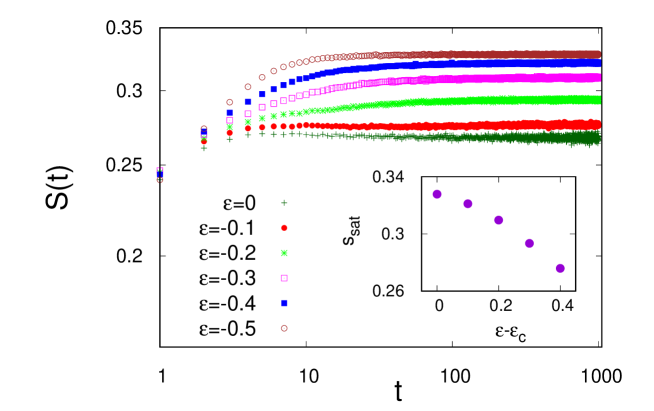
The probability of direction change of a particle is calculated by estimating the number of particles that changes direction of motion at time divided by the number of surviving particles at that time. Figure 8 shows the data for for different . For purely diffusive system , is independent of time, . is dependent on the dynamical updating rule, it turns out to be numerically with the asynchronous updating rule used here [16].
For , at first increases with time, then it reaches a constant value . Repulsion between the neighbouring particles is mainly responsible for the change in direction of motion. When decreases from zero the repulsive factor becomes stronger, particles change their direction more rapidly, increases. At the extreme limit , the change in direction is maximum as the particles perform nearly oscillatory motion. A systematic decrease of the saturation value is obtained when (calculated from the last 500 steps) are plotted against (see inset of figure 8).
.
3.2.3 Distribution of time interval spent without change in direction of motion
Another quantity calculated is , the probability distribution of the interval of time spent in between two successive changes in direction. A particle may continue to move in the same direction for different intervals of time denoted by . For each tagged particle, these intervals are calculated (up to a particular time ) to obtain the distribution at , which is normalised such that . Here we have calculated at .
For random walkers with , ) is given by
| (7) |
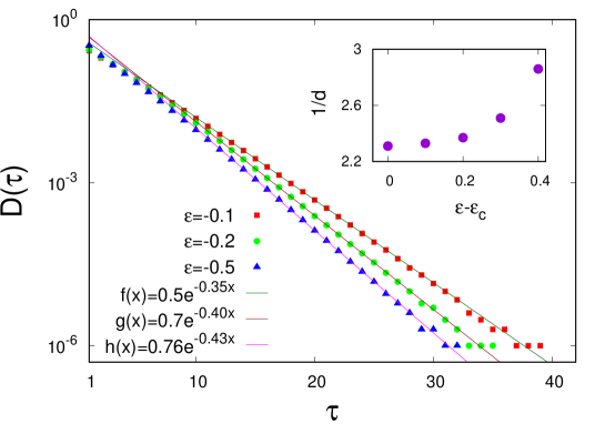
which reduces to an exponential form: . As for , is a constant at large times, is expected to show an exponential decay. Therefore, is fitted according to
| (8) |
Figure 9 shows the data for against for different values of calculated at time . is an effective ‘time scale’ which increases with , shown in the inset of figure 9 (calculated from the tail of the distribution). It shows that for , the tendency to oscillate is maximum.
In principle, the value of in equation (8) should be identical to . In order to check this, a careful inspection of the behaviour of shows that has a different value for small (up to ) and for the tail of the distribution. We have tabulated both the values obtained from the two regimes in Table 1 as well as the values of for comparison. Evidently, the values of the latter quantity match better with the values obtained from the smaller region of . This may be because for larger , the statistics is poorer as follows an exponential distribution. The discrepancy between the calculated value of from and that from large region of increases systematically with the magnitude of which may be because we are calculating ) at the same time for all .
| (for small ) | (for large ) | |||
|---|---|---|---|---|
| -0.1 | 0.276 | 0.323 | 0.320 | 0.350 |
| -0.2 | 0.293 | 0.347 | 0.346 | 0.400 |
| -0.3 | 0.310 | 0.371 | 0.370 | 0.423 |
| -0.4 | 0.321 | 0.387 | 0.383 | 0.430 |
| -0.5 | 0.328 | 0.396 | 0.397 | 0.431 |
4 Concluding remarks
In this paper, we have studied the behaviour of the model in one dimension, where the particles tend to avoid their nearest neighbour. The probability to move towards the nearest neighbour is taken parametrically as where . The case with has been studied earlier [14, 15, 16]. The bulk properties of the system show abrupt changes for any . In particular, a significant result in the present paper is that the fraction of surviving walker shows an inverse logarithmic decay for . Usually we find a power law decay in one dimension with possibly a logarithmic correction, e.g., in [22] and purely logarithmic in rare cases, an example in higher than two dimensions can be found in [23].
For the bulk properties (e.g., persistence probability, fraction of surviving particles) show universality in the sense there is a unique scaling behaviour of the dynamical quantities independent of . As a negative bias is incorporated in the system, both the fraction of surviving particles and persistence probability show a dependent behaviour. The persistence probability also does not show a power law dependence on time. The behaviour of the bulk properties can be qualitatively understood; the nature of the bias makes the particles more long lived and as a consequence, the probability of a site remaining unvisited decays faster than a power law.
At the microscopic level the system also shows completely different behaviour for positive and negative bias. First, the distributions have a different nature (Gaussian, single peaked) and also show a dependent scaling behaviour for the negative bias. Secondly, there is no crossover behaviour as found for the positive bias case. The negative bias case is entirely dominated by the repulsion from an early stage which causes rapid change of direction such that increases as becomes more negative.
For the fully biased case, , the motion is effectively the same as the repulsive motion between random walkers [20] where the scaling behaviour is known to be , which is also obtained from the simulations. Here we find in general ; an interesting issue is the dependence of on . The present results suggest that has a weak dependence on for ; it continuously decreases from to for . This has been confirmed using two different methods. We also find that ( corresponds to ) increases in a power law manner with . The fact that we get and not exactly 0.25 from Method II possibly indicates the presence of a finite size effect. On the other hand there is a sharp decay in the value of from 0.5 to as deviates from zero.
As already mentioned, for , the exponents are independent of while for , there is a non-universality. The former case is comparable to a system of charge-less massive particles with a variable gravitational interaction between nearest neighbours, the variation arising from the diffusive component. For the latter case when , the system resembles a collection of like charges with variable Coulomb interaction, the diffusive component again responsible for the variation. Of course, the annihilation factor is present in both cases such that a simple mapping to a system with gravitational or Coulomb interaction is not sufficient. For , in the extreme limit of , the diffusive component is absent and these charged particles may be regarded as electrons in a lattice perturbed from their equilibrium positions resulting in the well known oscillatory behaviour. This is because the particles attain a equidistant configuration at later times and the movements may be regarded as perturbations about their equilibrium positions.
For positive , the diffusive component does not affect the exponents and only causes a crossover behaviour while for , the diffusive component is more relevant as both the bulk and tagged particle dynamics show strong dependence. Hence, in a way, the gravitational interaction appears to be more ‘robust’ in comparison. The reason may be related to the fact that the annihilation factor is more effective for ; for , cases where the neighbours are equidistant occur more frequently, thereby enhancing the diffusive factor. This is evident from the snapshots even when is small in magnitude.
Acknowledgement: The authors thank DST-SERB project, File no. EMR/2016/005429 (Government of India) for financial support. Discussion with Purusattam Ray is also acknowledged.
5 ORCID iDs
Reshmi Roy https://orcid.org/0000-0001-6922-6858
Parongama Sen https://orcid.org/0000-0002-4641-022X
References
- [1] Privman V., ed. Nonequilibrium Statistical Mechanics in One Dimension, Cambridge University Press, Cambridge (1997).
- [2] Ligget T. M., Interacting Particle Systems, Springer-Verlag, New York, (1985).
- [3] Krapivsky P. L., Redner S. and Ben-Naim E., A Kinetic View of Statistical Physics, Cambridge University Press, Cambridge (2009).
- [4] Odor G., Rev. Mod. Phys. 76, 663 (2004).
- [5] Derrida B., J. Phys. A Math. Gen. 28, 1481 (1995).
- [6] Racz Z., Phys. Rev. lett. 55, 1707 (1985).
- [7] Amar J. G. and Family F., Phys. Rev. A 41, 3258 (1990).
- [8] ben-Avraham D., Burschka M. A., and Doering C. R., J. Stat. Phys. 60, 695 (1990).
- [9] Alcaraz F. C., Droz M., Henkel M. and Rittenberg V. , Ann. Phys. 230, 250 (1994).
- [10] Krebs K., Pfannmuller M. P., Wehefritz B. and Hinrinchsen H. , J. Stat. Phys. 78, 1429 (1995).
- [11] Santos J. E., Schutz G. M. and Stinchcombe R. B., J. Chem. Phys. 105, 2399 (1996).
- [12] Schutz G. M., Z. Phys. B 104, 583 (1997).
- [13] de Oliveira M. J., Brazilian Journal of Physics, 30 128 (2000).
- [14] Biswas S, Sen P and Ray P J. Phys.: Conf. Ser. 297, 012003 (2011).
- [15] Sen P and Ray P Phys. Rev. E 92, 012109 (2015).
- [16] Roy R, Ray P and Sen P J. Phys. A: Math. Theor. 53, 155002 (2020).
- [17] Biswas S and Sen P Phys. Rev. E 80, 027101 (2009).
- [18] Mullick P and Sen P Phys. Rev. E 99, 052123 (2019).
- [19] Derrida B, Bray A J and Godre’che C J. Phys. A 27, L357 (1994).
- [20] Arratia R Ann. Probab. 11 , 362 (1983).
- [21] Bhattacharjee S M and Seno F J. Phys. A: Math. Gen. 34 6375 (2001).
- [22] Dandekar R Phys. Rev E 97, 042118 (2018).
- [23] Ben-Naim E and Krapivsky P J. Phys. A 49, 504005 (2016).