Epitomic Variational Graph Autoencoder
Abstract
Variational autoencoder (VAE) is a widely used generative model for learning latent representations. Burda et al. [3] in their seminal paper showed that learning capacity of VAE is limited by over-pruning. It is a phenomenon where a significant number of latent variables fail to capture any information about the input data and the corresponding hidden units become inactive. This adversely affects learning diverse and interpretable latent representations. As variational graph autoencoder (VGAE) extends VAE for graph-structured data, it inherits the over-pruning problem. In this paper, we adopt a model based approach and propose epitomic VGAE (EVGAE), a generative variational framework for graph datasets which successfully mitigates the over-pruning problem and also boosts the generative ability of VGAE. We consider EVGAE to consist of multiple sparse VGAE models, called epitomes, that are groups of latent variables sharing the latent space. This approach aids in increasing active units as epitomes compete to learn better representation of the graph data. We verify our claims via experiments on three benchmark datasets. Our experiments show that EVGAE has a better generative ability than VGAE. Moreover, EVGAE outperforms VGAE on link prediction task in citation networks.
Index Terms:
Graph autoencoder , Variational graph autoencoder, Graph neural networks, Over-pruning, VAE, EVGAE.I Introduction
Graphs are data structures that model data points via nodes and the relations between nodes via edges. A large number of real world problems can be represented in terms of graphs. Some prominent examples are protein-protein interactions[6], social and traffic networks[9, 17] and knowledge graphs[8]. Deep learning applications related to graphs include but are not limited to link prediction, node classification, clustering [26, 28] and recommender systems[21, 1, 11].
Kipf and Welling [18] introduced variational graph autoencoder (VGAE) by extending the variational autoencoder (VAE) model [5]. Like VAE, VGAE tends to achieve the following two competing objectives:
-
1.
An approximation of input data should be possible.
-
2.
The latent representation of input data should follow standard gaussian distribution.
There is, however, a well-known issue with VAE in general: The latent units, which fail to capture enough information about the input data, are harshly suppressed during training. As a result the corresponding latent variables collapse to the prior distribution and end up simply generating standard gaussian noise. Consequently, in practice, the number of latent units, referred to as active units, actually contributing to reconstruction of the input data are quite low compared to the total available latent units. This phenomenon is referred to as over-pruning ([3, 2, 23]). Several solutions have been proposed to tackle this problem for VAEs. For instance, adding dropout can be a simple solution to achieve more active units. However, this solution adds redundancy rather than encoding more useful information with latent variables [27]. [14] proposes division of the hidden units into subsets and forcing each subset to contribute to the KL divergence. [2] uses KL cost annealing to activate more hidden units. [27] uses a model based approach where latent units are divided into subsets with only one subset penalized for a certain data point. These subsets also share some latent variables which helps in reducing the redundancy between different subsets.
VGAE, being an extension of VAE for graph datasets, is also susceptible to the over-pruning problem. This greatly reduces the modeling power of pure VGAE and undermines its ability to learn diverse and meaningful latent representations As demonstrated in detail in Sec. III. To suppress this issue, the authors of [18] simply reduce the weight of the second objective by the number of nodes in training data. For instance, PubMed dataset111PubMed is a citation dataset[22], widely used in deep learning for graph analysis. Details of the dataset are given in experiments Sec. VI-A has 20k nodes, so the second objective is given 20,000 times less weight than the first objective. Surprisingly, this factor is not mentioned in their paper, although it is present in their code [15]. Since the second objective is the one enforcing standard gaussian distribution for the latent variables, reducing its weight adversely affects the generative ability of VGAE and effectively reduces it to non-variational graph autoencoder. We discuss this further in Sec. IV.
In this work, we refer to VGAE without any weighted objective as pure VGAE to distinguish it from VGAE[18]. In order to attain good generative ability and mitigate over-pruning, we adopt a model based approach called epitomic VGAE (EVGAE). Our approach is motivated by a solution proposed for tackling over-pruning problem in VAE [27]. We consider our model to consist of multiple sparse VGAE models, called epitomes, that share the latent space such that for every graph node only one epitome is forced to follow prior distribution. This results in a higher number of active units as epitomes compete to learn better representation of the graph data. Our main contributions are summarized below:
-
•
We identify that VGAE[18] has poor generative ability due to the incorporation of weights in training objectives.
-
•
We show that pure VGAE (without any weighted objectives) suffers from the over-pruning problem.
-
•
We propose a true variational model EVGAE that not only achieves better generative ability than VGAE but also mitigates the over-pruning issue.
II Pure Variational Graph Autoencoder
Given an undirected and unweighted graph consisting of nodes with each node having features. We assume that the information in nodes and edges can be jointly encoded in a dimensional real vector space that we call latent space. We further assume that the respective latent variables follow standard gaussian distribution. These latent variables are stacked into a matrix . For reconstructing the input data, this matrix is then fed to the decoder network parameterized by . The assumption on latent representation allows the trained model to generate new data, similar to the training data, by sampling from the prior distribution. Following VAE, the joint distribution can be written as
| (1) |
where
| (2) | ||||
| (3) |
For an unweighted and undirected graph , we follow [18] and restrict the decoder to reconstruct only edge information from the latent space. The edge information can be represented by an adjacency matrix where refers to the element in row and column. If an edge exists between node and , we have . Thus, the decoder is given by
| (4) |
with
| (5) |
where denotes dot product and is the logistic sigmoid function.
The training objective should be such that the model is able to generate new data and recover graph information from the embeddings simultaneously. For this, we aim to learn the free parameters of our model such that the log probability of is maximized i.e.
| (6) |
where , parameterized by , models the recognition network for approximate posterior inference. It is given by
| (7) | ||||
| (8) |
where and are learnt using graph convolution networks (GCN) [17] and samples of are obtained from mean and variance using the reparameterization trick [5].
III Over-pruning in pure VGAE
Burda et al. [3] showed that learning capacity of VAE is limited by over-pruning. Several other studies [2, 23, 14, 27] confirm this and propose different remedies for the over-pruning problem. They hold the KL-divergence term in the loss function of VAE responsible for over-pruning. This term forces the latent variables to follow standard gaussian distribution. Consequently, those variables which fail to encode enough information about input data are harshly penalized. In other words, if a latent variable is contributing little to the reconstruction, the variational loss is minimized easily by “turning off” the corresponding hidden unit. Subsequently, such variables simply collapse to the prior, i.e. generate standard gaussian noise. We refer to the hidden units contributing to the reconstruction as active units and the turned-off units as inactive units. The activity of a hidden unit was quantified by Burda et al. [3] via the statistic
| (13) |
A hidden unit is said to be active if .
VGAE is an extension of VAE for graph data and loss functions of both models contain the KL-divergence term. Consequently, pure VGAE inherits the over-pruning issue. We verify this by training VGAE with Eq. (12) on Cora dataset222Details of Cora dataset are given in experiments Sec. VI-A. We employ the same graph architecture as Kipf and Welling [18]. The mean and log-variance of 16-dimensional latent space are learnt via Graph Convolutional Networks[17]. From Fig. 1(a), we observe that 15 out of 16 latent variables have KL-divergence around , indicating that they are very closely matched with standard gaussian distribution. Only one latent variable has managed to diverge in order to encode the information required by the decoder for reconstruction of the input.
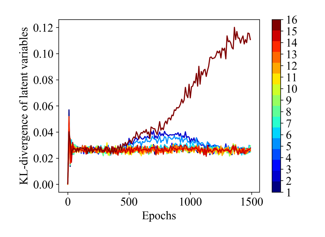
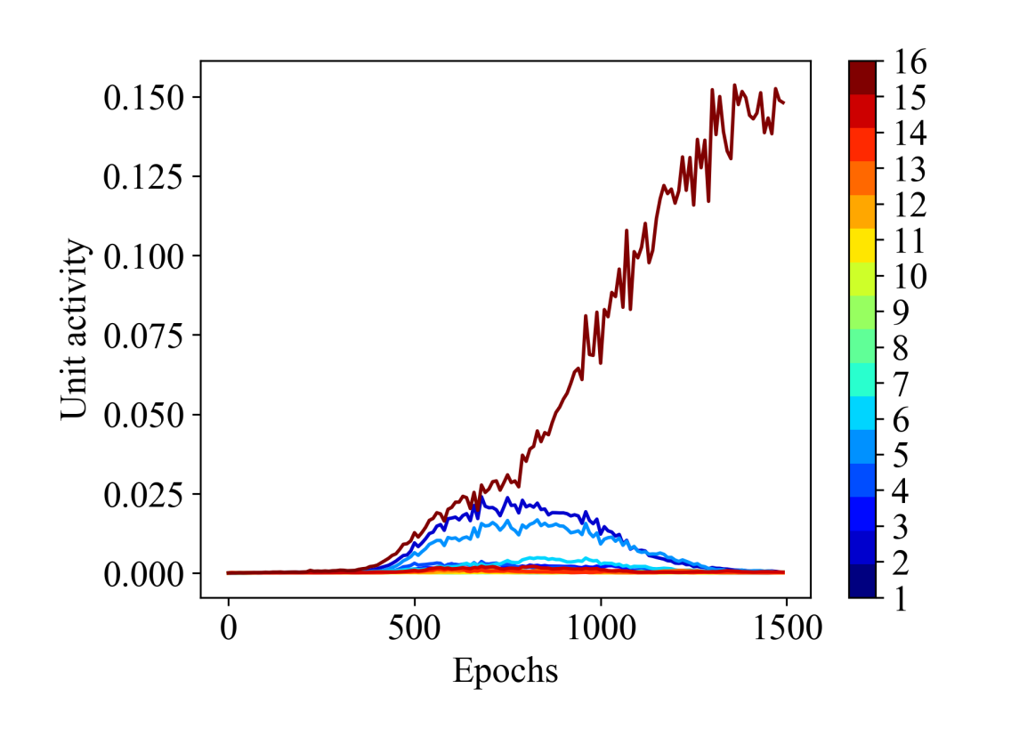
In other words pure VGAE model is using only one variable for encoding the input information while the rest 15 latent variables are not learning anything about the input. These 15 latent variables collapse to the prior distribution and are simply generating standard gaussian noise. Fig. 1(b) shows the activity of hidden units as defined in Eq. 13. It is clear that only one unit is active, which corresponds to the latent variable with highest KL-divergence in the Fig. 1(a). All other units have become inactive and are not contributing in learning the reconstruction of the input. This verifies the existence of over-pruning in pure VGAE model.
IV VGAE[18]: Sacrificing Generative Ability for Handling Over-pruning
Kipf and Welling’s VGAE[18] employed a simple way to get around the over-pruning problem by adding a penalty factor to the KL-divergence in Eq. (12). That is
| (14) |
But a consequence of using the penalty factor is poor generative ability of VGAE. We verify this by training VGAE on Cora dataset with varying in Eq. (14). We call the penalty factor , as the loss of VAE ( [10, 4] ) has the same factor multiplied with its KL-divergence term. Specifically, in VAE, is chosen to enforce better distribution matching. Conversely, a smaller is selected for relaxing the distribution matching, i.e. the latent distribution is allowed to be more different than the prior distribution. This enables latent variables to learn better reconstruction at the expense of the generative ability. In the degenerate case, when , VGAE model is reduced to non-variational graph autoencoder (GAE). VGAE as proposed by Kipf and Welling[18] has the loss function similar to VAE with chosen as reciprocal of number of nodes in the graph. As a result is quite small i.e. 0.0001-0.00001.
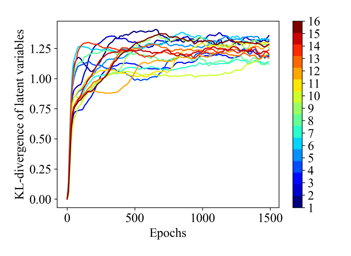
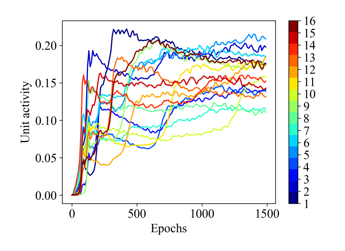
Fig. 2 shows the KL-divergence and hidden unit activity for original VGAE[18] model. We observe that all the hidden units are active, i.e. . However, the value of KL-divergence is quite high for all latent variables, indicating poor matching of with the prior distribution. This adversely affects the generative ability of the model. Concretely, the variational model is supposed to learn such a latent representation which follows standard gaussian (prior) distribution. Such high values of KL-divergence implies that the learnt distribution is not standard gaussian. The reason is that the KL-divergence term in (14) was responsible for ensuring that the posterior distribution being learned follows standard gaussian distribution. VGAE[18] model assigns too small weight ( = 0.0003) to the KL-divergence term. Consequently, when new samples are generated from standard gaussian distribution and then passed through the decoder , we get quite different output than the graph data used for training.
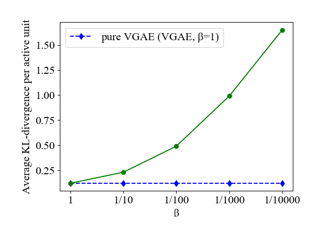
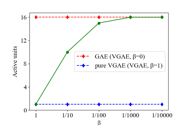
Fig. 3 shows that Kipf and Welling’s[18] approach to deal with over-pruning makes VAGE similar to its non-variational counter-part i.e. graph autoencoder (GAE). As is decreased, VGAE model learns to give up on the generative ability and behaves similar to GAE. This can be seen in Fig. 3 (a), where the average KL-divergence per active hidden unit increases drastically as becomes smaller. On the other hand, we observe from Fig. 3 (b) that decreasing results in higher number of active hidden units till it achieves the same number as GAE.
We conclude that as the contribution of KL-divergence is penalized in the loss function (Eq. 14), VGAE model learns to sacrifice the generative ability for avoiding over-pruning. Conversely, VGAE handles the over-pruning problem by behaving like a non-variational model GAE [16].
V Epitomic Variational Graph Autoencoder
We propose epitomic variational graph autoencoder (EVGAE) which generalizes and improves the VGAE model. EVGAE not only successfully mitigates the over-pruning issue of pure VGAE but also attains better generative ability than VGAE[18]. The motivation comes from the observation that for a certain graph node, a subset of the latent variables suffices to yield good reconstruction of edges. Yeung et al. [27] proposed a similar solution for tackling over-pruning problem in VAE. We assume subsets of the latent variables called epitomes. They are denoted by . Furthermore, it is ensured that every subset shares some latent variables with at least one other subset. We penalize only one epitome for an input node. This encourages other epitomes to be active. Let denote a discrete random variable that decides which epitome is penalized for a node . For a given node, the prior distribution of is assumed to be uniform over all the epitomes. represents the stacked random vector for all nodes of the graph. So:
| (15) |
where denotes uniform distribution.
Let denote a binary matrix, where each row represents an epitome and each column represents a latent variable. Fig. 4 shows with and in a -dimensional latent space. The grayed squares of row show the latent variables which constitute the epitome . We denote row of by .
V-1 Generative Model
of EVGAE is given by:
| (16) |
where
| (17) | ||||
| (18) |
where refers to component of epitome . Eq. (18) shows that follows standard gaussian distribution for the latent variables where and for the rest it follows degenerate distribution located at .
V-2 Inference Model
uses the following approximate posterior:
| (19) |
with
| (20) | |||
| (21) | |||
| (22) | |||
| (23) |
where refers to the categorical distribution. , and are learnt using two-layer GCN networks. Specifically, is obtained by learning a real vector which is then passed through softmax layer to give probabilities. Under the assumption that and are independent, given ; the objective function is given by
| (24) | ||||
| (25) | ||||
| (26) |
By using Jensen’s inequality [25], the ELBO bound for log probability becomes
| (27) | ||||
| (28) |
Following VGAE[18], we restrict the decoder to recover only edge information from the latent space. Hence, the decoder is the same as in Eq. (4). Thus, the first term in Eq. (28) simplifies in a similar way as in VGAE i.e. binary cross-entropy between input and reconstructed edges.
The second term in Eq. (28) is computed as:
| (29) |
The third term in Eq. (28) is computed as follows:
| (30) |
We take motivation from [27] to compute Eq. (30) as:
| (31) | ||||
| (32) |
where denotes component of vector . In Eq. (32), for each node, we sum over all the epitomes. For a given epitome, we only consider the effect of those latent variables which are selected by for that epitome. This also implies that the remaining latent variables have the freedom to better learn the reconstruction. Consequently, EVGAE encourages more hidden units to be active without penalizing the hidden units which are contributing little to the reconstruction. The final loss function is given by:
| (33) |
VGAE model can be recovered from EVGAE model, if we have only one epitome consisting of all latent variables. Hence the model generalizes VGAE. The algorithm for training EVGAE is given in Algo. 1.
-
•
-
•
Epochs
-
•
The matrix to select latent variables
VI Experiments
VI-A Datasets
We compare the performance of EVGAE with several baseline methods on the link prediction task. We conduct the experiments on three benchmark citation datasets[22].
Cora dataset has 2,708 nodes with 5,297 undirected and unweighted links. The nodes are defined by 1433 dimensional binary feature vectors, divided in 7 classes.
Citeseer dataset has 3,312 nodes defined by 3703 dimensional feature vectors. The nodes are divided in 6 distinct classes. There are 4,732 links between the nodes.
PubMed consists of 19,717 nodes defined by 500 dimensional feature vectors linked by 44,338 unweighted and undirected edges. These nodes are divided in 3 classes.
VI-B Implementation Details and Performance Comparison
In order to ensure fair comparison, we follow the experimental setup of Kipf and Welling[18]. That is, we train the EVGAE and pure VGAE model on an incomplete version of citation datasets. Concretely, the edges of the dataset are divided in training set, validation set and test set. Following [18], we use 85% edges for training, 5% for validation and 10% for testing the performance of the model.
We compare the performance of EVGAE with three strong baselines, namely: VGAE[18], spectral clustering[24] and DeepWalk[20]. We also report the performance of pure VGAE (=1) and GAE (VGAE with =0). Since DeepWalk and spectral clustering do not employ node features; so VGAE, GAE and EVGAE have an undue advantage over them. The implementation of spectral clustering is taken from [19] with 128 dimensional embedding and for DeepWalk, the standard implementation is used [7]. For VGAE and GAE, we use the implementation provided by Kipf and Welling[18]. EVGAE also follows a similar structure with latent embedding being 512 dimensional and the hidden layer consisting of 1024 hidden units, half of which learn and the other half for learning log-variance. We select 256 epitomes for all three datasets. Each epitome enforces three units to be active, while sharing one unit with neighboring epitomes. This can also be viewed as an extension of the matrix shown in Fig. 4. Adam [13] is used as optimizer with learning rate . Further implementation details of EVGAE can be found in the code [12].
For evaluation, we follow the same protocols as other recent works [18][20][24]. That is, we measure the performance of models in terms of area under the ROC curve (AUC) and average precision (AP) scores on the test set. We repeat each experiment 10 times in order to estimate the mean and the standard deviation in the performance of the models.
We can observe from Table I that the results of EVGAE are competitive or slightly better than other methods. We also note that the performance of variational method pure VGAE is quite bad as compared to our variational method EVGAE. Moreover, the performance of methods with no or poor generative ability (GAE and VGAE [18] with ) is quite similar.
VI-C EVGAE: Over-pruning and Generative Ability
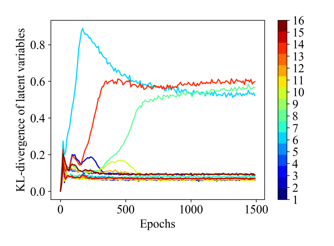
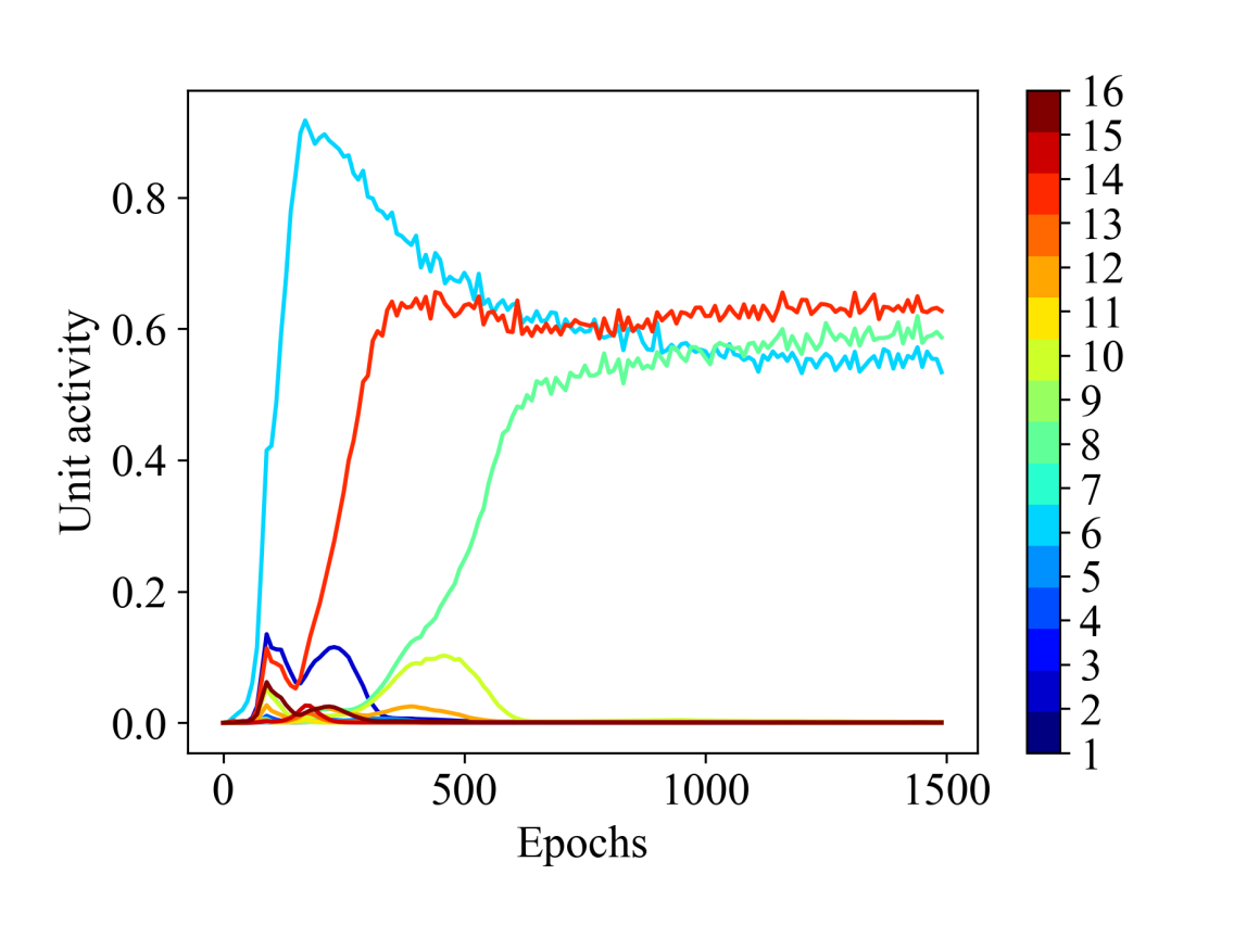
We now show the learning behavior of EVGAE model on our running example of Cora dataset. We select 8 epitomes, each dictating three hidden units to be active. The configuration is shown in Fig. 4. Fig. 5 shows the evolution of KL-divergence and unit activity during training of EVGAE model. By comparing this figure with pure VGAE (Fig. 1), we can observe that EVGAE has more active hidden units. This demonstrates that our model is better than pure VGAE at mitigating the over-pruning issue.
On the other hand, if we compare it to VGAE[18](Fig. 2), we observe EVGAE have less active units in comparison. But KL-divergence of the latent variables for VGAE is greater than 1 for all the latent variables (Fig. 2(a)). This implies that the latent distribution is quite different from the prior distribution (standard gaussian). In contrast, we observe from Fig. 5(a) that EVGAE has KL-divergence around 0.1 for 13 latent variables and approximately 0.6 for remaining 3 latent variables. This reinforces our claim that VGAE achieves more active hidden units by excessively penalizing the KL-term responsible for generative ability.
In short, although EVGAE has less active units, the distribution matching is better compared to VGAE. VGAE is akin to GAE due to such low weightage to KL-term, i.e. = 0.0003.
VI-D Impact of Latent Space Dimension
We now look at the impact of latent space dimension on the number of active units and average KL-divergence per active unit. We plot the active units for dimensions . Fig. 6 presents an overview of this impact on our running example (Cora dataset). For all values of , the number of epitomes is set to and one unit is allowed to overlap with neighboring epitomes. Similar to the configuration in Fig. 4 for . It is to be noted that we kept the same configuration of epitomes for consistency reasons. Choosing a different configuration of epitomes does not affect the learning behavior of EVGAE.
It can be observed that the number of active units is quite less compared to the available units for VGAE with (pure VGAE). Concretely, for only 48 units are active. This shows that the over-pruning problem persists even in high dimensional latent space.
Now we observe the behavior of VGAE with as proposed by Kipf and Welling[18], where denotes the number of nodes in the graph. All the units are active irrespective of the dimension of latent space. In the case of EVGAE, the number of active units is in between the two. i.e. we are able to mitigate the over-pruning without sacrificing the generative ability (). This results in better performance in graph analysis tasks as shown in table I.
To demonstrate that EVGAE achieves better distribution matching than VGAE, we compare the average KL-divergence of active units for different latent space dimensions. Only active units are considered when averaging the KL-divergence because the inactive units introduce a bias towards zero in the results. Fig. 6(b) shows how the distribution matching varies as we increase the number of dimensions. We note that when , the average KL-divergence for active units is still quite small, indicating a good match between learned latent distribution and the prior. Conversely, when the average KL-divergence per active unit is quite high. This supports our claim that original VGAE[18] learns a latent distribution which is quite different from the prior. Thus, when we generate new samples from standard gaussian distribution and pass it through the decoder, we get quite different output than the graph data used for training. In the case of EVGAE, the KL divergence is quite closer to the prior compared to VGAE. For , it is almost similar to the case with .
VII Conclusion
In this paper we looked at the issue of over-pruning in variational graph autoencoder. We demonstrated that the way VGAE [18] deals with this issue results in a latent distribution which is quite different from the standard gaussian prior. We proposed an alternative model based approach EVGAE that mitigates the problem of over-pruning by encouraging more latent variables to actively play their role in the reconstruction. EVGAE also has a better generative ability than VGAE[18] i.e. better matching between learned and prior distribution. Moreover, EVGAE performs comparable or slightly better than the popular methods for the link prediction task.
Acknowledgment
This work has been supported by the Bavarian Ministry of Economic Affairs, Regional Development and Energy through the WoWNet project IUK-1902-003// IUK625/002.
References
- [1] Peter Battaglia, Razvan Pascanu, Matthew Lai, Danilo Jimenez Rezende, et al. Interaction networks for learning about objects, relations and physics. In Advances in neural information processing systems, pages 4502–4510, 2016.
- [2] Samuel R Bowman, Luke Vilnis, Oriol Vinyals, Andrew M Dai, Rafal Jozefowicz, and Samy Bengio. Generating sentences from a continuous space. arXiv preprint arXiv:1511.06349, 2015.
- [3] Yuri Burda, Roger Grosse, and Ruslan Salakhutdinov. Importance weighted autoencoders. arXiv preprint arXiv:1509.00519, 2015.
- [4] Christopher P Burgess, Irina Higgins, Arka Pal, Loic Matthey, Nick Watters, Guillaume Desjardins, and Alexander Lerchner. Understanding disentangling in beta-vae. arXiv preprint arXiv:1804.03599, 2018.
- [5] Carl Doersch. Tutorial on variational autoencoders. arXiv preprint arXiv:1606.05908, 2016.
- [6] Alex Fout, Jonathon Byrd, Basir Shariat, and Asa Ben-Hur. Protein interface prediction using graph convolutional networks. In Advances in neural information processing systems, pages 6530–6539, 2017.
- [7] Aditya Grover and Jure Leskovec. node2vec: Scalable feature learning for networks. In Proceedings of the 22nd ACM SIGKDD international conference on Knowledge discovery and data mining, pages 855–864, 2016.
- [8] Takuo Hamaguchi, Hidekazu Oiwa, Masashi Shimbo, and Yuji Matsumoto. Knowledge transfer for out-of-knowledge-base entities: A graph neural network approach. arXiv preprint arXiv:1706.05674, 2017.
- [9] Will Hamilton, Zhitao Ying, and Jure Leskovec. Inductive representation learning on large graphs. In Advances in neural information processing systems, pages 1024–1034, 2017.
- [10] Irina Higgins, Loic Matthey, Arka Pal, Christopher Burgess, Xavier Glorot, Matthew Botvinick, Shakir Mohamed, and Alexander Lerchner. beta-vae: Learning basic visual concepts with a constrained variational framework. Iclr, 2(5):6, 2017.
- [11] Elias Khalil, Hanjun Dai, Yuyu Zhang, Bistra Dilkina, and Le Song. Learning combinatorial optimization algorithms over graphs. In Advances in Neural Information Processing Systems, pages 6348–6358, 2017.
- [12] Rayyan Ahmad Khan. Evgae. https://github.com/RayyanRiaz/EVGAE, 2020.
- [13] Diederik P Kingma and Jimmy Ba. Adam: A method for stochastic optimization. arXiv preprint arXiv:1412.6980, 2014.
- [14] Durk P Kingma, Tim Salimans, Rafal Jozefowicz, Xi Chen, Ilya Sutskever, and Max Welling. Improved variational inference with inverse autoregressive flow. In Advances in neural information processing systems, pages 4743–4751, 2016.
- [15] Thomas Kipf. gae. https://github.com/tkipf/gae/blob/716a46ce579a5cdba84278ccf71891d59e420988/gae/optimizer.py#L33.
- [16] Thomas Kipf. gae. https://github.com/tkipf/gae/issues/20#issuecomment-446260981.
- [17] Thomas N. Kipf and Max Welling. Semi-supervised classification with graph convolutional networks. 2016.
- [18] Thomas N Kipf and Max Welling. Variational graph auto-encoders. arXiv preprint arXiv:1611.07308, 2016.
- [19] Fabian Pedregosa, Gaël Varoquaux, Alexandre Gramfort, Vincent Michel, Bertrand Thirion, Olivier Grisel, Mathieu Blondel, Peter Prettenhofer, Ron Weiss, Vincent Dubourg, et al. Scikit-learn: Machine learning in python. Journal of machine learning research, 12(Oct):2825–2830, 2011.
- [20] Bryan Perozzi, Rami Al-Rfou, and Steven Skiena. Deepwalk: Online learning of social representations. In Proceedings of the 20th ACM SIGKDD international conference on Knowledge discovery and data mining, pages 701–710, 2014.
- [21] Alvaro Sanchez-Gonzalez, Nicolas Heess, Jost Tobias Springenberg, Josh Merel, Martin Riedmiller, Raia Hadsell, and Peter Battaglia. Graph networks as learnable physics engines for inference and control. arXiv preprint arXiv:1806.01242, 2018.
- [22] Prithviraj Sen, Galileo Namata, Mustafa Bilgic, Lise Getoor, Brian Galligher, and Tina Eliassi-Rad. Collective classification in network data. AI magazine, 29(3):93–93, 2008.
- [23] Casper Kaae Sønderby, Tapani Raiko, Lars Maaløe, Søren Kaae Sønderby, and Ole Winther. How to train deep variational autoencoders and probabilistic ladder networks. In 33rd International Conference on Machine Learning (ICML 2016), 2016.
- [24] Lei Tang and Huan Liu. Leveraging social media networks for classification. Data Mining and Knowledge Discovery, 23(3):447–478, 2011.
- [25] Eric W. Weisstein. Jensen’s inequality. From MathWorld—A Wolfram Web Resource.
- [26] Zonghan Wu, Shirui Pan, Fengwen Chen, Guodong Long, Chengqi Zhang, and Philip S Yu. A comprehensive survey on graph neural networks. arXiv preprint arXiv:1901.00596, 2019.
- [27] Serena Yeung, Anitha Kannan, Yann Dauphin, and Li Fei-Fei. Tackling over-pruning in variational autoencoders. arXiv preprint arXiv:1706.03643, 2017.
- [28] Jie Zhou, Ganqu Cui, Zhengyan Zhang, Cheng Yang, Zhiyuan Liu, Lifeng Wang, Changcheng Li, and Maosong Sun. Graph neural networks: A review of methods and applications. arXiv preprint arXiv:1812.08434, 2018.