A tomographic map of the large-scale matter distribution using the eBOSS - Stripe 82 Ly$\alpha$ forest

Abstract

The Lyman-$\alpha$ (hereafter Ly$\alpha$) forest is a probe of large-scale matter density fluctuations at high redshift, $z>2.1$. It consists of H i absorption spectra along individual lines-of-sight. If the line-of-sight density is large enough, 3D maps of H i absorption can be inferred by tomographic reconstruction. In this article, we investigate the Ly$\alpha$ forest available in the Stripe 82 field ($220\,\mathrm{deg^{2}}$), based on the quasar spectra from SDSS Data Release DR16. The density of observed quasar spectra is $37\,\mathrm{deg^{-2}}$ with a mean pixel signal-to-noise ratio of two per angstrom. This study provides an intermediate case between the average SDSS density and that of the much denser but smaller CLAMATO survey. We derive a 3D map of large-scale matter fluctuations from these data, using a Wiener filter technique. The total volume of the map is $0.94\,\mathrm{h^{-3}Gpc^{3}}$. Its resolution is $13\,\mathrm{h^{-1}Mpc}$, which is related to the mean transverse distance between nearest lines-of-sight. From this map, we provide a catalog of voids and protocluster candidates in the cosmic web. The map-making and void catalog are compared to simulated eBOSS Stripe 82 observations. A stack over quasar positions provides a visualization of the Ly$\alpha$ forest-quasar cross-correlation. This tomographic reconstruction constitutes the largest-volume high-redshift 3D map of matter fluctuations.

1 Introduction

Measuring the distribution of matter in the Universe is a major goal of observational cosmology. Features in this distribution provide information about the energy and matter content of the Universe as well as its gravitational evolution. The Ly$\alpha$ forest is a key probe of this distribution. It consists of absorptions in the electromagnetic spectrum of bright and distant sources such as quasars, due to the Ly$\alpha$ transition of intervening neutral hydrogen located at various redshifts along their lines-of-sight. As such, it provides a one-dimensional measurement of the amount of neutral hydrogen in the Intergalactic Medium (IGM) [1]. In this medium, the balance between processes such as photo-ionization by the ultraviolet background and electron recombination links the abundance of neutral hydrogen to the total baryon density. The latter is in turn correlated on large scales with the total matter distribution.

Quasars have been detected out to redshifts of 7.5 [2]. Ground-based observations provide Ly$\alpha$ forest measurements above $z=2.1$. The Ly$\alpha$ forest is one of the main probes of large-scale matter distribution at high redshift. Constraints on cosmological models, as well as on the neutrino mass, were obtained from the relatively small-scale 1D measurements of Ly$\alpha$ forest absorption [3, 4, 5, 6, 7]. Recently, the increase of both the line-of-sight density and observational footprint in large sky surveys allowed the measurement of 3-dimensional Ly$\alpha$ forest correlations [8]. In particular, the Ly$\alpha$ forest was used to measure the Baryon Acoustic Oscillation (BAO) scale through auto-correlation and cross-correlation with quasars [9, 10, 11, 12, 13, 14, 15].

While the Ly$\alpha$ forest data is one-dimensional by nature, it is possible to construct 3-dimensional maps from 1D data on scales comparable to the mean separation between lines-of-sight [16]. Such an endeavour was already performed by the COSMOS Ly$\alpha$ forest Mapping And Tomography Observations (CLAMATO) survey [17, 18, 19]. This program uses a dense set of spectroscopic observations from Lyman-break galaxies (LBGs) to reconstruct the cosmic web in a small area ($0.157\,\mathrm{deg^{2}}$). With a redshift range $z=2.05-2.55$, this survey provides a comoving volume of $30\times 24\times 438\,\mathrm{h^{-3}Mpc^{3}}$. With the combined use of LBGs and quasars, the achieved line-of-sight density is $1455\,\mathrm{deg^{-2}}$. The ultimate purpose of such high sampling programs is to outline the cosmic structure down to the scale of filaments, i.e. of the order of a Mpc. Accessing filament scales would be possible with future observations using e.g. the Extremely Large Telescope (ELT) [20]. The performance of the algorithm used by CLAMATO was assessed through cosmological simulations in [21, 22]. These studies determined in particular the map-making performance for different mean separation $\langle d_{\bot}\rangle$ between individual lines-of-sight.

In this article, we present a high-redshift Ly$\alpha$ forest absorption map on much larger scales, from part of the quasar spectra obtained by the Sloan Digital Sky Survey-IV (SDSS-IV) [23, 24, 25, 26]. They are provided by the 16^th Data Release (DR16) [27] of the SDSS Extended Baryon Oscillation Spectroscopic Survey (eBOSS). We use the same tomographic reconstruction algorithm developed by CLAMATO. The authors in [21] also exploited BOSS DR9 data to obtain a tomographic map, but with a lower line-of-sight density than in this study. Here we focus on the Stripe 82 part of the SDSS footprint (right ascension from 317°to 45°and declination from -1.25°to +1.25°).

Ly$\alpha$ forest tomographic mapping is already used for several applications. It has recently been applied to detect an enormous Ly$\alpha$ nebula on a very small portion of the sky [28] centered on the Ly$\alpha$ forest protoclusters found by the MAMMOTH project [29, 30]. Ly$\alpha$ forest tomography was also used to identify underdensities and overdensities in the matter distribution of the Universe. As an example, a $z=2.45$ protocluster was discovered in [31] and later confirmed as an overdensity of spectroscopically-observed galaxies. We perform a similar search with the tomographic map obtained in this article, and provide the most probable candidates for very large protocluster systems in the Stripe 82 field.

By applying a similar method to underdensities, large voids can be detected in the cosmic web. The statistical properties of voids provide an interesting probe for cosmology. For example, galaxy-based void catalogs were used, together with galaxies themselves, to improve Redshift Space Distortion (RSD) measurements with SDSS data [32, 33, 34]. One can produce an Alcock & Paczynski cosmological consistency test [35] by stacking voids and studying their profile (see e.g. [36, 37]). While several methods were developed to detect voids from galaxy surveys, detection based on the Ly$\alpha$ forest is less explored. It is possible to search for voids from the one-dimensional Ly$\alpha$ forest data, as shown in [38], but void searches based on 3D maps are clearly more efficient and robust, making use of redundant information from nearby lines-of-sight. A void search method based on tomographic Ly$\alpha$ forest mapping was developed in [39] and applied in [40] to produce a void catalog from the cosmic web. In this article, we apply a similar method to produce a catalog of void candidates from the Stripe 82 tomographic map. Given the volume and resolution of this map, we can retrieve large voids in the cosmic web.

This article is laid out as follows: Sect. 2 describes Ly$\alpha$ forest spectra available in eBOSS DR16, in the Stripe 82 footprint. Sect. 3 presents the method used to create our tomographic map. The quality of the map-making is assessed with dedicated simulations in Sect. 4. We describe methods to search for under- and overdensities in Sect. 5. Sect. 6 presents the tomographic map based on eBOSS data, together with its properties including the results of void and large overdensity searches, as well as the inferred stacked Ly$\alpha$ forest flux signal around quasars.

2 Lyman-alpha forest data

We use the Ly$\alpha$ forest region from quasar spectra available in the 16^th Data Release [27] (DR16) of the SDSS-IV eBOSS survey [23, 24, 25, 26]. The sky density of these objects, which is much smaller than that of LBGs, such as used by CLAMATO, is the main factor limiting the resolution of our tomographic map. For this reason, while the full eBOSS footprint could be used in principle, we choose here to focus on the Stripe 82 field, a narrow band in the Equatorial plane lying within the Southern Galactic Cap. In a large fraction of this field, a particularly dense and uniform sample of quasar spectra were acquired. Indeed, repeated photometric observations over a period of about ten years leads to targeting quasars and rejecting stellar contaminants in a particularly efficient way. This efficient selection was accomplished by combining the time-variability information from observed lightcurves together with color measurements [41, 42]. This improved targeting efficiency brings the mean quasar density in the Stripe 82 field to $37\,\mathrm{deg^{-2}}$. In comparison, with the same redshift range, the mean quasar density of the whole eBOSS footprint in DR16 is approximately $20\,\mathrm{deg^{-2}}$.

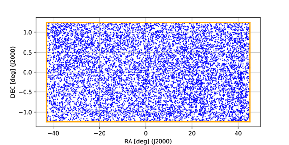
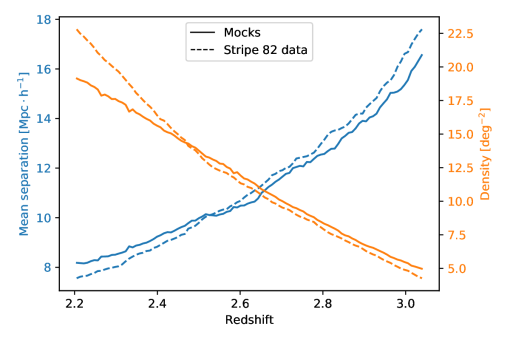
The footprint of our map within Stripe 82 is illustrated in Fig. 1. The right ascension range with a homogeneous Ly$\alpha$ forest dataset extends from -43°to +45°, and the declination covers Stripe 82 width, from -1.25°to +1.25°. This solid angle corresponds to $220\,\mathrm{deg^{2}}$. A total of 8199 Ly$\alpha$ forest spectra were obtained from quasar observations in this field, corresponding to the mean density of $37\,\mathrm{deg^{-2}}$. Lines-of-sight are selected over the redshift range $z=2.1-3.2$. Fig. 2 shows the mean line-of-sight effective density as a function of redshift. It also represents the mean separation $\langle d_{\bot}\rangle$ between nearest lines-of-sight as a function of redshift.

Figure 1: Sky distribution of the 8199 eBOSS - DR16 quasars in the Stripe 82 ($z=2.1-3.2$), which provide Ly$\alpha$ forest spectra for this study. The total density is $37\,\mathrm{deg^{-2}}$. The scales of the horizontal and vertical axes are different.

Figure 2: Blue: mean separation between nearest lines-of-sight [$\mathrm{h^{-1}Mpc}$] as a function of redshift. Orange: line-of-sight effective density [$\mathrm{deg^{-2}}$], as a function of redshift. DR16 data are shown in continuous curves while dashed curves correspond to mocks presented in Sect. 4. Higher difference at low redshift comes from the presence of high-noise quasars in the data which do not contribute quantitatively to the tomographic reconstruction. They are not modeled in the mocks.

Our quasar spectra originate from the SDSS DR16 Quasar catalog [43]. Quasar targets were observed over the five-year period from 2009 to 2014 during the BOSS survey [44, 45] or between 2014 and 2019 during the SDSS-IV eBOSS survey [23, 24]. Spectra were obtained by co-adding individual observations from typically four 15-minute long exposures. The spectra pixel size is of $1\,\mathrm{$\mathrm{\SIUnitSymbolAngstrom}$}$. An unbiased estimator for the observed flux $f(\lambda)$ is computed, weighting pixel data by the Charge Coupled Device (CCD) readout noise as in [13, 14]. For each spectrum, a Ly$\alpha$ forest flux contrast field $\delta_{F}(\lambda)$ (named flux contrast later) is defined by:

$$\delta_{F}(\lambda)=\frac{f(\lambda)}{C_{q}(\lambda)\overline{F}(z_{Ly\alpha})}-1.\\$$ (2.1)

In this expression $C_{q}(\lambda)$ is the unabsorbed quasar flux (the continuum), while $\overline{F}(z_{Ly\alpha})$ is the mean fraction of flux transmitted by the IGM at the redshift $z_{Ly\alpha}=\lambda/\lambda_{\alpha}-1$, such that by definition the average value of $\delta_{F}$ is zero at any redshift. The wavelength $\lambda_{\alpha}=1215.668\,\mathrm{$\mathrm{\SIUnitSymbolAngstrom}$}$ corresponds to the Ly$\alpha$ forest absorption peak at rest.

Following [13, 14, 46, 47], the Ly$\alpha$ forest flux contrasts are computed using the picca software, developed for the BOSS/eBOSS surveys. The product $C_{q}(\lambda)\overline{F}(z_{Ly\alpha})$ is evaluated directly with the same approach as in [13, 14]. Although the Stripe 82 field is smaller than the full BOSS footprint, the number of quasars in our Stripe 82 sample is large enough to use this approach. The quasar continuum is modeled as the product:

$$C_{q}(\lambda)=(a_{q}+b_{q}\log(\lambda))\,C\left(\lambda_{RF}=\frac{\lambda}{(1+z_{\rm quasar})}\right),$$ (2.2)

where $a_{q}$ and $b_{q}$ are quasar-dependent normalization terms. The parameters $a_{q}$, $b_{q}$, and $C(\lambda_{RF})$ are determined iteratively by normalizing $C(\lambda_{RF})$ for each redshift and maximizing a likelihood function.

We restrict the Ly$\alpha$ forest flux contrast calculation to pixels for which the observed wavelength is in the range $3769-5106\,\mathrm{$\mathrm{\SIUnitSymbolAngstrom}$}$, corresponding to $2.1<z<3.2$. We also select the rest-frame wavelength in the range $1040<\lambda_{RF}<1200\,\mathrm{$\mathrm{\SIUnitSymbolAngstrom}$}$, so that the measured flux fluctuations are dominated by the Ly$\alpha$ forest. In particular, we do not attempt to exploit the Lyman-$\beta$ forest at rest frame wavelengths below $1025\,\mathrm{$\mathrm{\SIUnitSymbolAngstrom}$}$. The cut $\lambda_{RF}<1200\,\mathrm{$\mathrm{\SIUnitSymbolAngstrom}$}$ implies that for a given line-of-sight the closest selected pixel is located on average $49\,\mathrm{h^{-1}Mpc}$ from the associated quasar. This decision mitigates most of the proximity effect: close to a quasar, the proportion of neutral hydrogen is indeed influenced by the large UV radiation background [48].

In addition to the flux contrast $\delta_{F}$, picca provides an estimate of the instrumental noise $\sigma_{\delta_{F}}$. The corresponding signal-to-noise ratio per pixel $\mathrm{SNR}=F/\sigma_{F}=(\delta_{F}+1)/\sigma_{\delta_{F}}$ is typically close to 2. This value is relatively large compared to the case of CLAMATO. One of the main reason of this difference is that SDSS quasars are considerably brighter than typical LBGs.

Broad Absorption Line (BAL) quasar spectra are not used. We use the balnicity index of the CIV absorption [49, 50], removing quasars whose balnicity index is larger than zero. This suppress 6% of quasars and is not counted in the 8199 quasars.

The flux contrast $\delta_{F}$ is also contaminated by High Column Density (HCD) objects such as Damped Ly$\alpha$ forest systems (DLAs) [51]. These typically originate from the lines-of-sight passing near foreground galaxies. Although HCD objects by themselves constitute tracers of the matter distribution, they have a specific bias and an extended impact on the observed spectra. For simplicity we therefore choose to mask the affected regions of the spectra.

To remove HCD contaminations, we use the DR16 HCD catalog obtained with the finder dla_cnn [52]. This machine learning algorithm identifies candidate HCDs together with inferred H i column density and a detection confidence parameter. Among the candidates, we select those whose column density is $N_{\rm HI}>10^{19.7}\,\mathrm{cm^{-2}}$ with a detection confidence larger than 70 %. This limit corresponds to most DLAs, defined by $N_{\rm HI}>2\times 10^{20}\,\mathrm{cm^{-2}}$ [51], and some Super Lyman Limit Systems, defined by $19<\mathrm{log}_{10}(N_{\rm HI}/\mathrm{cm^{-2}})<20.3$ [53]. In practice for our data set the HCD detection efficiency is poor for $\mathrm{log}_{10}(N_{\rm HI}/\mathrm{cm^{-2}})<20.3$. We remove the pixels where the estimated HCD-induced absorption is higher than 20 %. The fraction of Ly$\alpha$ forest pixels lost by this cut is 11 %. In addition, the absorption in the corresponding Lorentzian-profile damping wings that remain after the cut are corrected with a Voigt profile following [13]. The resulting set of ($\delta_{F}$, $\sigma_{\delta_{F}}$), as a function of sky coordinates and redshift, constitutes the input data to the next step of tomographic map-making.

3 Tomographic map-making algorithm

Tomographic reconstruction algorithms can be used to infer the 3-dimensional IGM density from a set of 1-dimensional Ly$\alpha$ forest line-of-sight. In [54, 55], several techniques are presented to adapt tomographic methods to the creation of a 3D Ly$\alpha$ forest flux map. In [54], a Bayesian method is presented. An advanced use of Bayesian methods in this context is also given in [56] and [57], which apply a dynamic forward modelling approach to model the observed 1D lines-of-sight and reconstruct the 3D density and velocity fields of the IGM.

Under certain hypotheses detailled in [54], the Bayesian approach is mathematically equivalent to applying a Wiener filter [58, 59]. Wiener filtering provides an unbiased minimum-variance linear estimator of a field. A simple implementation of this method, adapted to Ly$\alpha$ forest datasets, was developed by CLAMATO [17, 18, 19, 39, 60]; and our work uses the same public code, DACHSHUND. An advantage of this approach is its technical simplicity: it does not rely on complex assumptions for the underlying model, but still includes the effects of instrumental properties of the input data.

Since the mean separation between nearest lines-of-sight in our dataset is of the order of $10\,\mathrm{h^{-1}Mpc}$, we aim to reconstruct a map with a resolution close to this value. Therefore only large-scale Ly$\alpha$ forest flux (or matter) fluctuations are retained in the reconstructed map. Their distribution is nearly Gaussian, so the underlying linear model used for Wiener filtering is well adapted to our case. In fact, [19] found that Wiener filtering, with adapted parameters, is appropriate even in the case of the CLAMATO survey whose line-of-sight density is much larger than that of eBOSS.

The Wiener filter takes as an input the 1D line-of-sight data $\mathbf{d}$, assumed to be the sum of pixel signals $\mathbf{s}_{p}$ and Gaussian noise $\mathbf{n}$:

$$\mathbf{d}=\mathbf{s}_{p}+\mathbf{n}\ .$$ (3.1)

The Wiener filter provides an estimate, $\mathbf{\hat{s}}=\mathbf{L}\cdot\mathbf{d}$, for the Ly$\alpha$ forest flux contrast signal over the entire volume by minimizing the difference between the reconstructed signal $\mathbf{\hat{s}}$ and the signal of the input pixels in the map called $\mathbf{s}_{m}$:

$$\epsilon=E[|\mathbf{s}_{m}-\mathbf{\hat{s}}|^{2}]\ .$$ (3.2)

The minimization, detailed e.g., in [54], results in the expression for the operator $\mathbf{L}=\mathbf{S_{mp}}(\mathbf{S_{pp}}+\mathbf{N})^{-1}$. Here, the pixel-pixel and map-pixel covariance matrices $\mathbf{S_{pp}}$ and $\mathbf{S_{mp}}$ are both modeled by Gaussian kernels:

$$\mathbf{S}_{ij}=\sigma_{F}^{2}\exp\left(-\frac{(r_{i\parallel}-r_{j\parallel})^{2}}{2L_{\parallel}^{2}}\right)\exp\left(-\frac{(r_{i\bot}-r_{j\bot})^{2}}{2L_{\bot}^{2}}\right),$$ (3.3)

where $L_{\bot}$ and $L_{\parallel}$ are the transverse and longitudinal correlation lengths of the signal, which is discussed below. The parameter $\sigma_{F}^{2}$ is the expected variance of flux fluctuations in the map; in practice, it controls the amplitude of fluctuations in the reconstructed map. For our data, the noise matrix $\mathbf{N}$ is well approximated by a diagonal matrix with $\mathbf{N}_{ii}=n_{i}$, where $n_{i}$ is the individual pixel noise of pixel $i$.

The DACHSHUND public code makes use of a conjugate gradient Wiener filter. We convert the line-of-sight angular and redshift coordinates into pixel coordinates $(x,y,z)$ that represent angular, right ascension for $x$ and declination for $y$, and longitudinal, $z$, comoving distances, in $\mathrm{h^{-1}Mpc}$. We assume the concordance $\mathrm{\Lambda CDM}$ cosmology with fixed $\Omega_{\Lambda}=0.6853$, $\Omega_{m}=0.3147$, according to [61]. Since all coordinates are expressed in $\mathrm{h^{-1}Mpc}$, no assumption on the value of $H_{0}$ is needed. As mentioned in [19], the choice of cosmology only affects the global longitudinal and transverse scales.

It is technically convenient to define the $(x,y,z)$ approximated coordinate system such that all lines-of-sight are parallel to each other, and the output map is a rectangular box. For that reason, comoving angular distances are computed for all pixels using the same redshift $z=2.65$ corresponding to the middle redshift. The spread in declination of the input data is 2.5°, so that distance errors between the lowest and highest redshifts $z=2.1$ to 3.2 are of the order of a few percent along the $y$-axis of the map. In the right ascension direction, 88° wide, the difference is much larger as the parallel approximation does not hold at all. Therefore, without any supplementary coordinate transformations, this map is not adapted for studies on large-scale distances.

The DACHSHUND input is a list of pixels vectors $(x,y,z,\delta_{F},\sigma_{\delta_{F}})$. It is used to construct $(r_{\parallel},r_{\bot},\mathbf{d},\mathbf{N})$ following the definition of the Wiener filter. The output is a 3D map containing the reconstructed Ly$\alpha$ forest flux $\delta_{\mathrm{Fmap}}$ that corresponds to the signal $\hat{s}$. The map is pixellized at approximately one pixel per $\mathrm{h^{-1}Mpc}$.

Wiener filter tomographic reconstruction is not a parameter-free method. The main parameters are the normalization $\sigma_{F}$, and the transverse $L_{\bot}$ and longitudinal $L_{\parallel}$ smoothing lengths. The transverse $L_{\bot}$ correlation length is constrained by the fact that no transverse Ly$\alpha$ forest flux fluctuations can be reconstructed with a size smaller than the mean separation $\langle d_{\bot}\rangle$ between nearest lines-of-sight. Fig. 2 shows the evolution of this quantity as a function of redshift. The transverse correlation length increases with redshift in a way related to the redshift distribution of quasar sources used in the sample. From this figure, we choose $L_{\bot}=13\,\mathrm{h^{-1}Mpc}$, so that $L_{\bot}>\langle d_{\bot}\rangle(z)$ for $z<2.8$, which covers most of the map. At high redshift, $z>2.8$, $L_{\bot}$ is smaller than the mean line-of-sight separation, a fact which must be considered when interpreting the map.

In principle, the longitudinal smoothing length $L_{\parallel}$ could be set at a value close to a Mpc, which corresponds to the spectrograph resolution. However, since this value is much smaller than $\langle d_{\bot}\rangle$ we choose to set $L_{\parallel}=L_{\bot}=13\,\mathrm{h^{-1}Mpc}$. This choice reduces the amplitude of anisotropies in the Wiener-filtered map, and keeps large-scale information while removing small-scale longitudinal fluctuations of the Ly$\alpha$ forest flux.

Another parameter to choose is the normalization factor $\sigma_{F}$, which controls the contrast of the map. The maximal reconstructed density contrasts are controlled by the ratio $\sigma_{F}^{2}/n_{\rm min}^{2}$, where $n_{\rm min}$ is the minimal value of the diagonal elements of the noise matrix $\mathbf{N}$ [60]. Indeed, in order to avoid numerical divergences in the Wiener filter algorithm, these matrix elements must be bounded by a floor value. Given the statistical distribution of pixel noise in our dataset, we adopt $n_{\rm min}=0.1$, so that for the 6.3 % of the pixels with lowest noise, this minimum value is used rather than the true pixel noise for the corresponding elements $n_{i}$. In the CLAMATO analysis, $n_{\rm min}$ was set to 0.2 due to larger relative noise in LBG spectra [19]. As for CLAMATO, we choose $\sigma_{F}^{2}$ such that the maximal contrast of the Wiener-filtered map is 1, which implies $\sigma_{F}^{2}=0.01$.

Finally, for computational reasons, the map-making procedure is parallelized by dividing the Stripe 82 field into chunks, and merging the corresponding sub-maps at the end of reconstruction. To avoid edge effects, we allow the chunks to overlap, with an overlap width of $L_{\bot}$. This technique allows one to process large data samples without adding numerical artifacts.

The result of the tomographic reconstruction over the whole Stripe 82 is a map with $(5856\times 180\times 834)$ pixels. Its total size in terms of $(x,y,z)$ coordinates, in the right ascension, declination, redshift directions, is $(6352\times 180\times 835)\,\mathrm{h^{-3}Mpc^{3}}$. The corresponding comoving volume, computed without parallel line-of-sight approximation, is $0.94\,\mathrm{h^{-3}Gpc^{3}}$.

4 Mocks and algorithm validation

4.1 Map-making on adapted simulations

To assess the performance of tomographic reconstruction, we do not use physical simulations of the Ly$\alpha$ forest, as they require hydrodynamical effects and a resolution on the order of 100 kpc. No such simulation exists covering a near-Gpc³ volume. Instead, we use much simpler synthetic data, called mocks, based on Gaussian random fields. Such mocks [62, 63, 64] have been developed to reproduce the observed statistical properties of the Ly$\alpha$ forest on relatively large scales, over BOSS or DESI (Dark Energy Spectroscopic Instrument [65]) footprints. These properties include the 3D auto-correlation function or the cross-correlation with other matter tracers, such as quasars.

We briefly summarize here the creation of these mocks. Gaussian fields are generated in a Fourier space box. The modes of this box are multiplied by several sets of appropriate weights such that, after applying an inverse 3D Fourier transform, they produce several boxes: a box of matter density fluctuations, $\delta_{m}$, at $z=0$; six boxes of velocity gradient components at $z=0$; and a box of quasar density fluctuations at $z=2.3$. A quasar catalogue is obtained by placing a quasar in each cell of this last box with a probability proportional to the logarithm of the density in the cell. For our study, this step was adapted in order to match the sky density and redshift distribution of eBOSS-DR16 quasars in Stripe 82, as described in Sect. 2. The Ly$\alpha$ forest transmitted-flux-fraction, $F$, along the line-of-sight to each quasar is finally obtained following the Fluctuating Gunn-Peterson [66] approximation, i.e., $F=\exp(-\tau)$, where the optical depth $\tau$ reads :

$$\tau=a(z)\exp\left[-b\,G(z)\,(\delta_{m}+\delta_{s}+c(z)\,\eta_{\parallel})\right].$$ (4.1)

In this expression, the field $\delta_{s}$ is added to $\delta_{m}$ in order to take into account small-scale flux fluctuations that are missing due to the relatively large, 2$h^{-1}$ Mpc, size of the box pixels. It is tuned to match the observed 1D power spectrum of the Ly$\alpha$ forest. The velocity gradient along the line-of-sight, $\eta_{\parallel}$, is obtained from the velocity-gradient component boxes. The parameters $a(z)$ and $c(z)$ are adjusted to match the observed Ly$\alpha$ forest bias and $\beta$ parameters. The parameter $c(z)$ controls redshift space distortions, and its value is actually close to $\beta$. $a(z)$ controls the bias. We set $b=2-0.7(\gamma-1)=1.58$, for an equation-of-state parameter of the intergalactic medium $\gamma=1.6$ [67]. Finally, $G(z)$ is the linear growth factor at the redshift of the considered pixel, with the convention $G(z=0)=1$.

Figure 3: Normalized histograms of the flux contrast pixel noise $\sigma_{\delta_{F}}$ , for both our selected Stripe 82 data and mocks. A pixel corresponds to the flux contrast over $1\,\mathrm{$\mathrm{\SIUnitSymbolAngstrom}$}$ width.

The flux is multiplied by a continuum to produce a quasar spectrum, and metals and HCD systems are added to the spectra using the quickquasars program. HCD systems are then removed with the same method as for the data, as detailed in Sect. 2. The final outputs of the simulation are spectra and an associated quasar catalogue, over a footprint matching our Stripe 82 selection. BAL quasars are not included in mock spectra. The mock spectra are then treated with the same pipeline and parameters as the DR16 spectra detailed in Sect. 2.

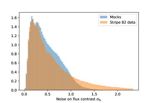
Figure 2 illustrates the agreement between mocks and data with respect to the line-of-sight separation as a function of redshift. The histogram of flux-contrast noise, $\sigma_{\delta_{F}}$, is presented for mocks and our selected data in Fig. 3. The average and standard deviations of the noise distributions are similar, but their shapes are significantly different, especially at low signal-to-noise ratio. This result is related to the fact that the number of high magnitude quasars is smaller for mocks than in the DR16 data. However, the difference in the high-noise tail has a minor impact on the tomographic map, because Wiener filtering assigns more weight to low-noise pixels. We checked this effect explicitly, by constructing maps for which high-noise data were removed. This result is in agreement with [19, 60].

Figure 4: Slice through the tomographic Ly$\alpha$ forest flux map derived from mock data. It covers a 22°right-ascension range (along the $x$ axis), at fixed declination. The filtering parameters are described in Sect. 3. Circles are the intersection between the represented slice and identified voids. Filled (empty) stars represent quasars whose distance along the $y$ axis is less than 5 (10) $\mathrm{h^{-1}Mpc}$ from the slice. Lines-of-sight used for the tomographic reconstruction are pictured as full (dotted) lines if they are 5 (10) $\mathrm{h^{-1}Mpc}$ from the slice.

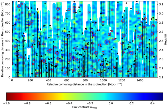
We apply the tomographic algorithm described in Sect. 3 to all mock data. Fig. 4 displays a slice of one quarter of the Stripe 82 mock map. The reconstructed Ly$\alpha$ forest flux contrast, $\delta_{\mathrm{Fmap}}$, is represented by a color map such that matter overdensities, corresponding to negative flux contrast, appear in red, while matter underdensities are in blue. Map pixels further than $20\,\mathrm{h^{-1}Mpc}$ from any lines-of-sight are masked, as they can not be reasonably reconstructed; they appear in white in the representation.

4.2 Performance of the matter density reconstruction

Since the reconstructed map of Ly$\alpha$ forest flux contrast traces flux fluctuations on scales larger than $13\,\mathrm{h^{-1}Mpc}$, it is expected to be an accurate representation of the associated matter fluctuations at similar scales. In order to estimate to what extent our tomographic map reproduces the underlying field of matter fluctuations, we use the reconstructed map of flux contrast $\delta_{\mathrm{Fmap}}$ from mock data and compare it to the input field of matter fluctuations $\delta_{\mathrm{m}}$. This random field was computed as a first step during mock data production. The field $\delta_{\mathrm{m}}$ is interpolated into the cartesian grid of the tomographic map. Since the original $\delta_{\mathrm{m}}$ was computed at $z=0$, it is multiplied by the linear growth factor at the considered redshift. Finally, $\delta_{m}$ is Gaussian smoothed with a smoothing length of $8\,\mathrm{h^{-1}Mpc}$, which was chosen in order to optimize the correlation signal with the tomographic Ly$\alpha$ forest map.

Figure 5: Comparison between the reconstructed flux contrast from our simulation and the input underlying field of matter fluctuations. The redshift range $z=2.1-2.7$ is considered. The map of matter density fluctuations was Gaussian smoothed over $8\,\mathrm{h^{-1}Mpc}$. White ellipses represent the $1\sigma$ and $2\sigma$ contours of a 2D Gaussian fit to the distribution.

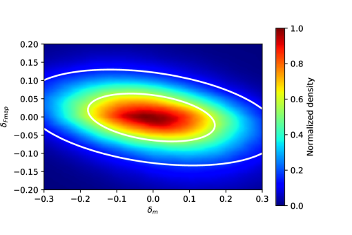
The resulting smoothed map of matter fluctuations is compared to the tomographic Ly$\alpha$ forest flux contrast map $\delta_{\mathrm{Fmap}}$ in Fig. 5. At high redshifts, a large fraction of the map is masked, therefore we restrict the comparison to the redshift range $z=2.1$ to $2.7$.

The correlation coefficient between both fields is $r=-0.34$. This number provides the simplest estimation of the ability of our tomographic approach to map the underlying cosmological field of matter fluctuations, and can be compared to simulation-based results of [22]. They tested several signal-to-noise ratios and line-of-sight separations and reported a correlation coefficient of $56\%$ for the closest values to our dataset ($\langle d_{\bot}\rangle=12.65\,\mathrm{h^{-1}Mpc}$ and signal-to-noise ratio of 2). Their correlation coefficient, however, was computed relative to the initial Ly$\alpha$ forest fluxes, not to the underlying density fields. We can also compare our correlation factor with results from weak-lensing tomography of large-scale matter fluctuations. In particular, [68] used wide-field weak-lensing observations to construct a 3D tomographic map of matter fluctuations for $z=0.1-1$ over a 167 deg² field. The comparison with matter density fluctuations as traced by galaxies yielded a correlation coefficient $r\sim 10$ %.

As demonstrated in the simulations of [22], the correlation of the tomographic map with the underlying matter field would naturally improve with smaller $\langle d_{\bot}\rangle$ and, to a smaller extent, larger signal-to-noise.

5 Identification of underdensities and overdensities

Since the computed tomographic Ly$\alpha$ forest flux contrast map is anti-correlated with matter density fluctuations, an immediate application is to search for large under- and overdensities in the mapped volume.

5.1 Overdensity search

Protoclusters are defined as structures that will, at some stage, collapse into a galaxy cluster. At $z>2$, protoclusters are expected to be ubiquitous in the cosmic web, and to have a characteristic radius of 6 Mpc [69] for the largest ones. It is clear that, from the tomographic map produced in this study, only overdensities with a typical scale larger than $13\,\mathrm{h^{-1}Mpc}$ can be identified. We may therefore expect, from our tomographic map, to be able to identify the largest protoclusters from $z=2.1$ to $z=3.2$ in the Stripe 82 field. Based on the study of [60], we designed a watershed search algorithm, similar to the one used by [31] to detect protoclusters in the CLAMATO survey.

We search for large deficit in the Ly$\alpha$ forest flux contrast to identify overdensities. In the watershed algorithm, all pixels whose $\delta_{\mathrm{Fmap}}$ is smaller than a given threshold, $\delta_{ws}$, are selected and then sorted into groups of neighbours. For each cluster, the center is defined as the pixel with the lowest $\delta_{\mathrm{Fmap}}$. We define the cluster radius by $R_{\mathrm{overdensity}}=(3N_{\mathrm{pixel}}V_{\mathrm{pixel}}/4\pi)^{1/3}$ where $N_{\mathrm{pixel}}$ is the number of pixels contributing to the cluster, and $V_{\mathrm{pixel}}$ is the pixel volume. In addition, clusters whose radius is smaller than a fixed parameter $R_{\mathrm{min}}$ are removed. The output of the algorithm is a catalog of overdensities characterized by a central position and a radius.

In the protocluster search presented in [60], the CLAMATO tomographic map is smoothed beforehand at a $4\,\mathrm{h^{-1}Mpc}$ scale, matching the dimension of searched protoclusters. In our case, we are limited by the $13\,\mathrm{h^{-1}Mpc}$ smoothing length of our map, so this step is not needed. The threshold $\delta_{ws}$ impacts both the positions and the radii of overdensities. As in [39], we set $\delta_{ws}=-3.5\,\tilde{\sigma}_{\delta_{\mathrm{Fmap}}}$, where $\tilde{\sigma}_{\delta_{\mathrm{Fmap}}}$ is the measured standard deviation of the tomographic map. The minimum cluster radius is set to $R_{\mathrm{min}}=7\,\mathrm{h^{-1}Mpc}$ so that identified overdensities have a diameter larger than the smoothing length of the map.

Finally, in order to mitigate the impact of residual HCD systems and metals which could generate spurious overdensity detections (see e.g. [29]), we require that each selected cluster be crossed by lines-of-sight whose total length of crossing is larger than three times the cluster diameter. This criterion implies that each overdensity candidate is crossed by more than three lines-of-sight.

We stress again that only very extended overdensities in the cosmic web can be detected using our tomographic map. Interpreting their properties, in particular in terms of candidate protoclusters, would require dedicated N-body simulations, a task beyond the scope of this article. Applying our overdensity search procedure to the mock tomographic map results in the identification of nine candidates. Their mean radius is $10.5\,\mathrm{h^{-1}Mpc}$. The values of the underlying matter density fluctuations, averaged within the overdensity radii, are positive for all candidates, with a mean value $\langle\delta_{M}\rangle=0.4$.

5.2 Void finding method

Voids are underdensities in the cosmic matter field located between filaments and walls. Their typical size is approximately $10\,\mathrm{h^{-1}Mpc}$ [36], but they have a wide distribution of dimensions. With a tomographic map smoothed at a scale of $13\,\mathrm{h^{-1}Mpc}$, we can identify large voids. The near-Gpc volume covered by Stripe 82 makes such a search particularly useful. The Ly$\alpha$ forest tomographic map is an opportunity to study the feasibility of void cosmology at high redshift with the Ly$\alpha$ forest [60, 39].

We adopt a simple-spherical algorithm to identify voids. The approach is more robust than the watershed algorithm with respect to noise on large scales as the watershed algorithm tends to provide complex void shapes [39].

The simple-spherical method selects all the pixels that have a flux contrast $\delta_{\mathrm{Fmap}}$ larger than a threshold $\delta_{th}$. At each selected point, a sphere is grown in radius until the mean flux value $\langle\delta_{\mathrm{Fmap}}\rangle$ inside the sphere reaches an average limit $\delta_{av}$. After treating all the selected pixels, some voids overlap. For each group of overlapping voids, the selection is done iteratively. The void with the largest radius is kept and all the spheres directly overlapping this void are suppressed. Groups of overlapping spheres are repeatedly created and the aforementioned procedure is applied until all remaining voids are separated. Voids with a radius smaller than a certain value $R_{\mathrm{min}}$ are deleted.

As for the watershed method, this algorithm relies on a few parameters on which the output void catalogs strongly depend. The parameter $\delta_{th}$ mainly controls the depth of the voids while $\delta_{av}$ controls the profile of the void, i.e., its size. The parameters $\delta_{av}$ and $\delta_{th}$ must be chosen simultaneously because of their correlated impacts on the void selection. If the value of threshold $\delta_{th}$ is too low, the centers of the detected voids are offset relative to the maximal $\delta_{\mathrm{Fmap}}$ inside the void. If $\delta_{th}$ is too high, only the deepest voids are detected. For reasonable values of $\delta_{th}$, modifying $\delta_{av}$ globally changes the void radius but does not move the center positions. Finally, $R_{\mathrm{min}}$ is used to select voids with a radius larger than the smoothing length of the map.

We adjusted the void detection parameters by applying the void finder to our mock tomographic map, in a similar approach to [39]. The minimal radius is fixed at $R_{min}=7\,\mathrm{h^{-1}Mpc}$, identical to the minimal overdensity radius. Scanning over different algorithm parameters, we choose $\delta_{th}=0.14$ and $\delta_{av}=0.12$. With this choice the positions of large voids, of $\sim 25\,\mathrm{h^{-1}Mpc}$ radius, are stable when varying the parameters around the central values.

Two additional criteria are applied to selected voids in order to remove those located in areas where the tomographic reconstruction is not able to operate without extrapolating. Similarly to the analysis of overdensities, we require that each selected void is crossed by lines-of-sight with a total length larger than the void radius. This constraint implies in particular that selected voids are crossed by at least two lines-of-sight. In addition, we require that for each selected void, less than 5 % of its volume is located in the masked region, i.e., more than $20\,\mathrm{h^{-1}Mpc}$ distant from any line-of-sight.

After applying these criteria, the void filling factor, defined as the ratio of the total void volume over the total map volume, is 14 %, similar to the value of 15 % found by [39].

5.3 Properties of identified voids in mock data

The results of our void finding procedure on the mock tomographic map is presented in Fig. 4, where identified voids are represented by circles. The distribution of voids is rather uniform over the map. The largest reconstructed void radius from mock data is $34$ $\mathrm{h^{-1}Mpc}$ as can be seen in Fig. 10 (right).

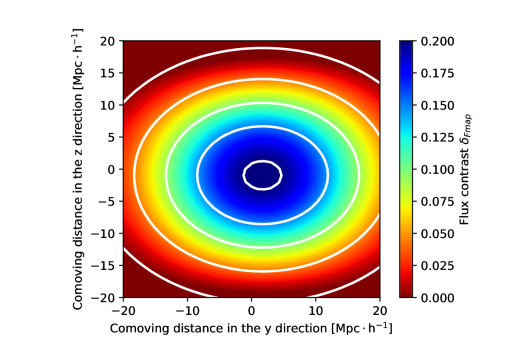
It is possible to estimate the average shape of the reconstructed Ly$\alpha$ forest flux within voids. As smaller voids are likely to be more contaminated by noise fluctuations, we focus on voids with reconstructed radius larger than $L_{\bot}=13\,\mathrm{h^{-1}Mpc}$. From the mock tomographic map, we compute an average 3-dimensional void profile by stacking the map around all identified void centers, using the appropriate comoving coordinate system. The result is illustrated in Fig. 6. Contours are smooth due to the large number of voids detected over a near-Gpc³ volume. In the $x-y$ plane (perpendicular to the lines-of-sight) the void profile has a circular shape. However, as shown in Fig. 6, it is clearly anisotropic in the $y-z$ plane: voids are more extended perpendicularly to the lines-of-sight. To quantify this effect, we fit the stacked void profile by a 2-dimensional Gaussian function. Axis ratios in the $x-y$, $y-z$ and $x-z$ planes are defined by $d_{ij}=\sigma_{i}/\sigma_{j}$ where $\sigma_{k}$ is the standard deviation of the 2D Gaussian along the axis $k$. Statistical error bars on these $d_{ij}$ are computed with the Jackknife resampling method. The measured axis ratios are $d_{yz}=1.37\pm 0.01$ and $d_{xz}=1.36\pm 0.01$. As a reference, the axis ratio in the $x-y$ plane is $d_{xy}=0.98\pm 0.005$.

There are three plausible causes to this $\sim 36$ %-level anisotropy:

• An error in the choice of coordinate system, or equivalently in the underlying cosmological model, can generate an anisotropy in the average void profile - the Alcock-Paczynski effect [35]. Unless drastically departing from the coordinate system implied by existing contraints on cosmological parameters ([61]), such an effect cannot explain the observed axis ratio. We also checked that our use of conventional $(x,y,z)$ coordinate system, described in Sect. 3, instead of true comoving coordinates, does not modify the observed axis ratio.

• Redshift-space distortions (RSD) are present in the Ly$\alpha$ forest flux, and taken into account in mocks by the term $c(z)\,\eta_{\parallel}$ in Eqn. 4.1. To assess their impact on the average mock void profile, we computed a dedicated mock where the term $c(z)\,\eta_{\parallel}$ is suppressed. Its axis ratio is $d_{yz}=1.33$, smaller than when RSD are included ($d_{yz}=1.37\pm 0.01$). This result demonstrates that RSD do impact the observed void anisotropy, but are not a dominant factor.

• While the Wiener filter algorithm we adopted is isotropic in itself ($L_{\parallel}=L_{\bot}$), the input distribution of line-of-sight pixels is strongly anisotropic, with straight, parallel lines-of-sight. The tomographic map inherits this anisotropy. For example, by artificially subsampling the input line-of-sight mock data, the statistical isotropy of the corresponding pixels is increased and the mean void axis ratio is decreased. This behavior indicates that a large fraction of the mean void axis ratio is due to this effect.

Figure 6: Stacked profile of voids identified in the mock data, with radii larger than $13\,\mathrm{h^{-1}Mpc}$. The stack is over all the Stripe 82 field, with RSD effects included. White ellipses represent contours of a Gaussian fit to the profile.

6 Results on eBOSS data

6.1 Tomographic map and properties of voids

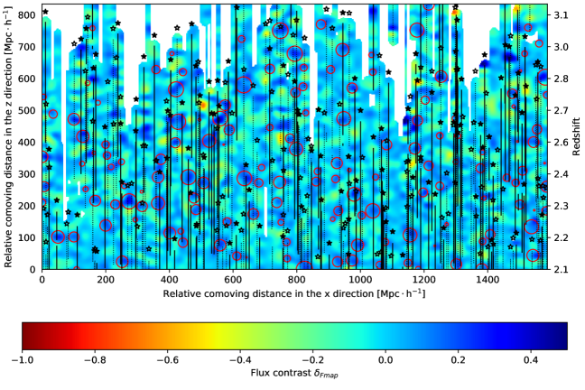
We apply the algorithm detailed in Sect. 3 on the selected eBOSS - DR16 dataset presented in Sect. 2, with the same parameters and output format as those for the mock map presented in Sect. 4. In particular, pixels located more than $20\,\mathrm{h^{-1}Mpc}$ from any given line-of-sight are masked.The resulting map is available on Zenodo. Fig. 7 presents a constant-declination slice of this map over one quarter of the Stripe 82 field.

Figure 7: Slice of the tomographic map computed from the observed eBOSS Ly$\alpha$ forest fluxes in the Stripe 82. The slice is at constant declination $\delta_{J2000}=0\degree$, and covers RA $\in[1\degree,23\degree]$, i.e., roughly a quarter of the Stripe 82 field. The lines-of-sight, quasars, and voids are represented as in Fig. 4. All pictured quasars and line-of-sights (full and dotted) are located in a $20\mathrm{h^{-1}Mpc}$-thick slice. This thickness corresponds to $0.28\degree$ in the declination direction.

Figure 8: 3D representation of the tomographic map over the entire Stripe 82, in spherical coordinates. Red (blue) iso-surfaces of flux contrast $-0.2$ ($0.2$) represent overdensities (underdensities). The corresponding 3D interactive representation is available on: https://skfb.ly/6RyGL. An interactive representation of overdensities is available on: https://skfb.ly/6RyGE.

Figure 9: 3D representations of portions of the Stripe 82 field. Top: $2.5\degree\times 2.5\degree$ field in right ascension and declination. Red (blue) iso-surfaces of flux contrast $-0.2$ ($0.2$) represent overdensities (underdensities). Lines-of-sight are represented in black. Bottom: $7\degree\times 2.5\degree$ field in right ascension and declination. Blue iso-surfaces of flux contrast 0.14 represent underdensities, at the same level than searched by the void finder ($\delta_{th}$). Identified voids are represented by light grey spheroids. The corresponding 3D interactive representations are available on https://skfb.ly/6RyGn (top) and https://skfb.ly/6RyGP (bottom).

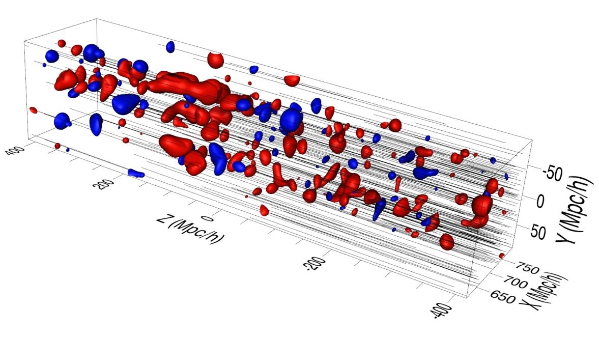
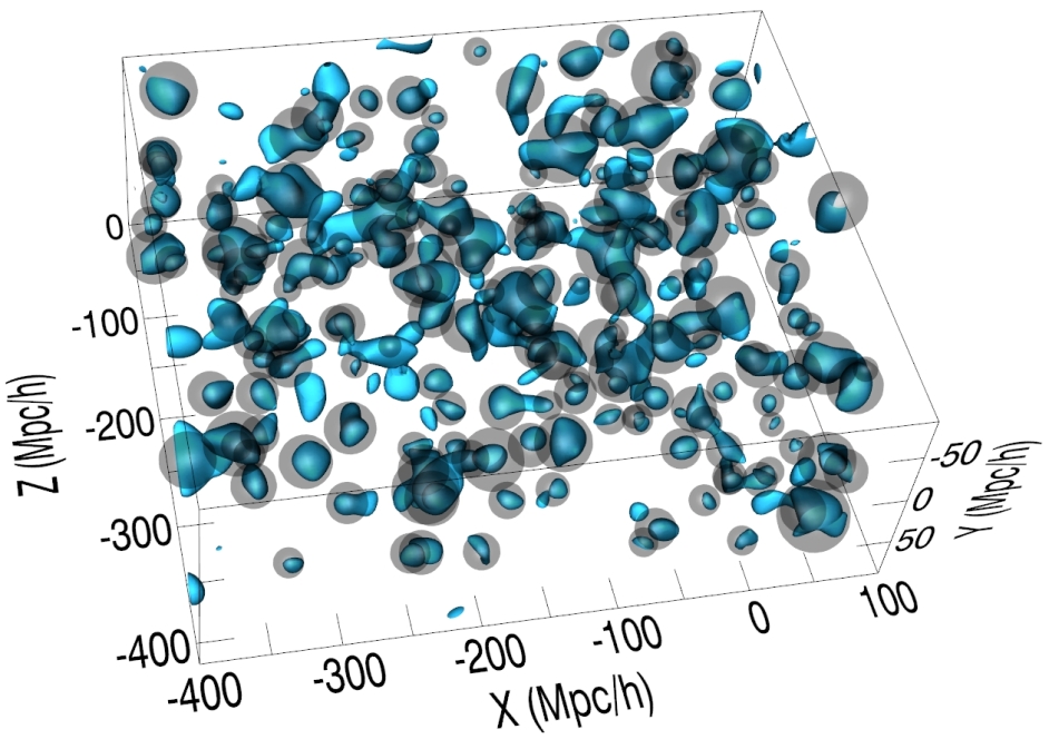
In addition we provide 3D representations of the tomographic map. Some visualizations were prepared with the Saclay Data Visualization (SDvision) [70] software deployed in the IDL environment, and also provide interactive web-based visualizations hosted on the Sketchfab platform. The SDvision software allows for the interactive and immersive visualization of scalar and vector fields, clouds of points, as well as ancillary datasets such as the lines-of-sight and catalogues of reconstructed voids. In our representations, the Ly$\alpha$ forest flux contrast is visualized using isocontour 3D surfaces at negative and positive values to indicate overdense and underdense regions, respectively. Sketchfab is a web-based service that enables the sharing of 3D models. The user can rotate, pan, zoom in and out regions of interest, and benefit from GPU acceleration through the WebGL API, as well as immersive Virtual Reality capabilities in association with VR headsets. Examples and links to these 3D interactive animations are given in Fig. 8 and 9. All the corresponding 3D interactive animations are available on https://sketchfab.com/pomarede/collections/eboss-paper.

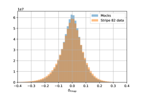
The flux contrast distribution in the reconstructed map is presented and compared to that of the mock map in Fig. 10 (left). Both histograms are well approximated by a Gaussian distribution; however, we observe a higher standard deviation in the data distribution than in the mocks. This result may be related to the difference in noise distribution that we pointed out in Fig. 3.

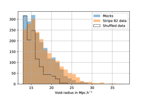
Large voids in the matter distribution are identified by applying the void finder algorithm on the Stripe 82 data with the same parameters as described in Sect. 5.2. The voids are represented by circles on the slice view of Fig. 7. A catalog providing void coordinates and dimensions is available on Zenodo${}^{\ref{zenodo_data_release}}$. A total of 439 void candidates are detected in Stripe 82 with a radius larger than $20\,\mathrm{h^{-1}Mpc}$. The distribution of void radii is shown in Fig. 10 (right), and compared to that of mock data. For both Stripe data and mocks, a tail of distribution is observed. The profile is well fit by an exponential law $dN/dR\sim\exp(-R/R_{0})$, with $R_{0}=4.9\pm 0.3\,\mathrm{h^{-1}Mpc}$ ($5.6\pm 0.3$) for data (mocks). This feature of the distribution is expected and comparable to the measured statistical properties of low-redshift voids, e.g., [71].

In order to investigate the physical origin of our large-void tail of distribution, we shuffled the line-of-sight pixels randomly from the initial $\delta_{F}$ data, keeping the line-of-sight positions fixed. After map-construction and void finding, the resulting void radius distribution is shown in Fig. 10 (right, dashed line). The high-radius tail observed in data is absent after shuffling: the number of voids with a radius larger than $20\,\mathrm{h^{-1}Mpc}$ is 6 % of the one observed in non-shuffled data. For void candidates with radii $\lesssim 15\,\mathrm{h^{-1}Mpc}$, the contamination from noise fluctuations is important. This result indicates that low radius voids are contaminated by false positive detections. As a comparison, in the galaxy field, random Poisson point distribution gives very similar results concerning the distribution of voids [32, 33].

Comparing mocks and data, a Kolmogorov-Smirnov test demonstrates that the mock and data void radius distributions are not compatible with each other, with more large voids in the data than in the mocks. This difference might arise from differences between noise distributions or the modelization of synthetic HCD systems in the mocks.

Figure 10: Comparison between tomographic map properties derived from the mocks and for eBOSS DR16 data. Left: Histogram of the Ly$\alpha$ forest flux contrast. Right: Histogram of void radii (for radii larger than $L_{\bot}=13\,\mathrm{h^{-1}Mpc}$). Dashed line represent void radii obtained after shuffling the input data, see Sect. 6.

6.2 Matter overdensities

We now present the result of searches for matter overdensities in the tomographic map, both a blind search and searches around known objects.

In the Stripe 82 field, the only large and homogeneous sample of known objects with $z>2.1$ and accurate (spectroscopic) redshift determination are the quasars actually used as targets for BOSS/eBOSS Ly$\alpha$ forest flux measurements. Fig. 11 displays our Stripe 82 tomographic Ly$\alpha$ forest flux stacked around quasars in the same field, with $z=2.1-3.2$. We observe a 3-dimensional signal, extending over roughly $20\,\mathrm{h^{-1}Mpc}$. By stacking on random map positions, the central signal of this stacked map produces a $5.2\sigma$ excess with respect to a random distribution. This result is a recast view of the small-separation part of the cross-correlation between quasar positions and Ly$\alpha$ forest flux described in [14, 15]. The statistical significance of the signal is, however, smaller, since this study is limited to the Stripe 82 field.

Figure 11: Stacked tomographic Ly$\alpha$ forest map centered around quasars over Stripe 82. Left: View in the $y-z$ plane. The mean line-of-sight position with respect to the quasar is represented by a red line, at the bottom of the image at $y=0$. Right: view in the $x-y$ plane.

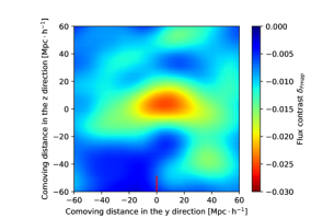
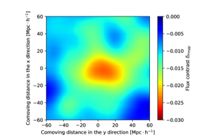
Since quasars are by definition located at the end of lines-of-sight, there is a concern that the observed cross-correlation signal is biased by the Wiener filtering algorithm itself. However, the tomographic Ly$\alpha$ forest flux is peaked right at the quasar position, within statistical uncertainties, whereas the lines-of-sight used for the reconstruction are located on average $49\,\mathrm{h^{-1}Mpc}$ away, i.e., 3 times the width $L_{\bot}$ of the filtering kernel. Such a bias, if any, is therefore a minor effect.

A hint for anisotropy in the stacked signal around quasars is visible in the $y-z$ slice in Fig. 11. The asymmetry of the signal along the lines-of-sight is smaller than its sky-coordinate extension. Using the same method as in Sect. 5.3, we find that the axis ratios of the stacked signal are $d_{xy}=0.68\pm 0.15$, $d_{xz}=2.31\pm 0.23$, and $d_{yz}=2.52\pm 0.63$, with statistical error bars estimated by Jackknife resampling.

We computed the same stack around quasars in the mock map; the corresponding axis ratios are $d_{xy}=0.77\pm 0.16$, $d_{xz}=1.79\pm 0.06$, and $d_{yz}=2.18\pm 0.10$. The anisotropy observed in the data is therefore statistically sound, and compatible with predictions from simulations. The origin of this anisotropy may be, as in the case of voids presented in Sect. 5.3, a combination of numerical effects in the map-making procedure and RSD. The proximity effect should not be responsible for this anisotropy, since it was not taken into account in our mock sample.

We also examined the correlation of the tomographic map with DLAs. We applied the same stacking procedure as was done for quasars, centering on the positions of identified DLAs in the Stripe 82, with $N_{\rm HI}>10^{20.3}\,\mathrm{cm^{-2}}$. There is an $2.6\,\sigma$ deficit of tomographic Ly$\alpha$ forest flux at the DLA positions. The signal is clearly fainter than for quasars as there is an order of magnitude less detected DLAs.

We now turn to a blind search for overdensities. This search aims at identifying candidate high-redshift protoclusters or more generally large overdensities over the wide Stripe 82 field. As detailed in Sect. 5.1, we apply the watershed algorithm on the Stripe 82. The adopted threshold is $\delta_{ws}=-3.5\,\tilde{\sigma}_{\delta_{\mathrm{Fmap}}}=-0.273$, where the standard deviation of the flux contrast of the map $\tilde{\sigma}_{\delta_{\mathrm{Fmap}}}$ is computed by using a Gaussian fit of the $\delta_{\mathrm{Fmap}}$ distribution.

These criteria yield eight selected overdensities in the tomographic map; table 1 lists their properties. Their average estimated radius is $12\,\mathrm{h^{-1}Mpc}$; as expected, they correspond to particularly large, and massive, protocluster candidates. The number of candidate overdensities is compatible with that found from the mock map in Sect. 5.1. Assessing in more detail the completeness and robustness of this selection would require the use of N-body simulations adapted to the identification of protocluster halos, which is beyond the scope of this article.

	1	2	3	4	5	6	7	8
RAJ2000 [deg]	-37.621	-27.442	3.1647	33.792	38.748	41.031	41.481	41.421
DECJ2000 [deg]	0.583	-0.166	0.472	0.750	-1.166	-0.0276	-0.528	-0.0276
Redshift	2.734	2.818	2.525	2.435	2.377	3.170	2.111	2.764
Radius [$\mathrm{h^{-1}Mpc}$]	15.13	10.54	13.88	10.68	9.081	7.623	16.20	12.77
Radius [arc min.]	12.56	8.75	11.52	8.869	7.539	6.329	13.45	10.60
Minimal $\delta_{\mathrm{Fmap}}$	-0.76	-0.44	-0.69	-0.63	-0.38	-0.40	-0.74	-0.54

Table 1: Properties of selected overdensities (protocluster candidates) over all the volume of our Stripe 82 tomographic map.

7 Conclusion

From the BOSS and eBOSS quasar spectra measured within the Stripe 82 field, we constructed a near-Gpc³ volume 3D tomographic map of the Ly$\alpha$ forest flux contrast. Its $13\,\mathrm{h^{-1}Mpc}$ resolution is such that it directly maps the large-scale distribution of matter, both baryonic and dark. This map is a unique representation of matter fluctuations at high redshifts $z>2$ over such a volume.

From synthetic data, we evaluate a $-34\%$ correlation coefficient of the tomographic map with respect to the underlying matter fluctuations, smoothed over $8\,\mathrm{h^{-1}Mpc}$. This value is comparable to other estimations based on N-body simulation [22].

We presented a search for large voids over the volume of the map. There is a reasonable match between the statistical properties of voids in mocks and Stripe 82 data; in particular, we unveil a tail of distribution of voids in comoving radius, reaching up to $\sim 30\,\mathrm{h^{-1}Mpc}$. The void geometry in the tomographic map is not isotropic. While mocks demonstrate that a small fraction of their axis ratio originates from RSD, most of it arises from the line-of-sight geometry of Ly$\alpha$ forest data.

Stacking the tomographic map around quasars yields a clear cross-correlation signal, with amplitude and shape in agreement with simulations including the RSD effect. The map is also well adapted to protocluster searches with radius larger than $7\,\mathrm{h^{-1}Mpc}$; we provide a list of candidates identified by a watershed algorithm.

Unlike the CLAMATO map [18, 19], the SDSS line-of-sight density is not sufficient to investigate the filamentary structure of the cosmic web. However, with the explored volume, this SDSS tomographic map allows the identification of potential large cosmic voids and overdensities with unprecedented statistical power. Compared to weak-lensing tomography, e.g., [68], Ly$\alpha$ forest tomographic maps can better estimate the matter distribution in the longitudinal direction, which is limited by the width of the lensing kernel in the case of weak lensing.

There are several avenues for improvement, both in terms of methodology and data. First, more advanced algorithms can be used, in particular following the forward modelling approach [56, 57]. Other technical improvements are also possible, such as including the Lyman-$\beta$ region of the spectra.

Cross-correlation studies with other tracers are currently limited given the high redshift range of our analysis. Ongoing and future surveys will address this issue, with applications, for example, in the search for protoclusters. The tomographic map in itself could be used for several cosmological analysis different from the typical correlation function-based approach, e.g., advanced shape analysis of over- and under-densities could lead to other cosmological constraints.

Finally, while this study focuses on the Stripe 82 field as observed with SDSS data, future work will be dedicated to studies of other fields, in particular making use of the upcoming DESI [65] and WEAVE-QSO [72] surveys. For these two surveys, mean line-of-sight separation down to $7\,\mathrm{h^{-1}Mpc}$ can be achieved in very dense regions, and will lead to more extended and more refined tomographic maps.

References

- [1] R. A. C. Croft, D. H. Weinberg, N. Katz and L. Hernquist, Cosmology from the structure of the Lyman alpha forest, in 12th Potsdam Cosmology Workshop: Large Scale Structure: Tracks and Traces: International Workshop Potsdam, Germany, September 15-20, 1997, 1997, astro-ph/9801255.
- [2] E. Bañados, B. P. Venemans, C. Mazzucchelli, E. P. Farina, F. Walter, F. Wang et al., An 800-million-solar-mass black hole in a significantly neutral Universe at a redshift of 7.5, Nature 553 (2018) 473 [1712.01860].
- [3] U. Seljak, A. Slosar and P. McDonald, Cosmological parameters from combining the Lyman-alpha forest with CMB, galaxy clustering and SN constraints, JCAP 0610 (2006) 014 [astro-ph/0604335].
- [4] N. Palanque-Delabrouille, C. Yèche, J. Lesgourgues, G. Rossi, A. Borde, M. Viel et al., Constraint on neutrino masses from SDSS-III/BOSS Ly forest and other cosmological probes, JCAP 2 (2015) 45 [1410.7244].
- [5] N. Palanque-Delabrouille et al., Neutrino masses and cosmology with Lyman-alpha forest power spectrum, JCAP 1511 (2015) 011 [1506.05976].
- [6] C. Yèche, N. Palanque-Delabrouille, J. Baur and H. du Mas des Bourboux, Constraints on neutrino masses from Lyman-alpha forest power spectrum with BOSS and XQ-100, JCAP 1706 (2017) 047 [1702.03314].
- [7] N. Palanque-Delabrouille, C. Yèche, N. Schöneberg, J. Lesgourgues, M. Walther, S. Chabanier et al., Hints, neutrino bounds and WDM constraints from SDSS DR14 Lyman- and Planck full-survey data, 1911.09073.
- [8] A. Slosar, A. Font-Ribera, M. M. Pieri, J. Rich, J.-M. Le Goff, É. Aubourg et al., The Lyman- forest in three dimensions: measurements of large scale flux correlations from BOSS 1st-year data, JCAP 2011 (2011) 001 [1104.5244].
- [9] N. G. Busca, T. Delubac, J. Rich, S. Bailey, A. Font-Ribera, D. Kirkby et al., Baryon acoustic oscillations in the Ly forest of BOSS quasars, A&A 552 (2013) A96 [1211.2616].
- [10] A. Slosar, V. Iršič, D. Kirkby, S. Bailey, N. G. Busca, T. Delubac et al., Measurement of baryon acoustic oscillations in the Lyman- forest fluctuations in BOSS data release 9, JCAP 2013 (2013) 026 [1301.3459].
- [11] BOSS collaboration, Quasar-Lyman Forest Cross-Correlation from BOSS DR11 : Baryon Acoustic Oscillations, JCAP 1405 (2014) 027 [1311.1767].
- [12] BOSS collaboration, Baryon acoustic oscillations in the Ly forest of BOSS DR11 quasars, Astron. Astrophys. 574 (2015) A59 [1404.1801].
- [13] J. E. Bautista et al., Measurement of baryon acoustic oscillation correlations at with SDSS DR12 Ly-Forests, Astron. Astrophys. 603 (2017) A12 [1702.00176].
- [14] H. du Mas des Bourboux et al., Baryon acoustic oscillations from the complete SDSS-III Ly-quasar cross-correlation function at , Astron. Astrophys. 608 (2017) A130 [1708.02225].
- [15] M. Blomqvist et al., Baryon acoustic oscillations from the cross-correlation of Ly absorption and quasars in eBOSS DR14, Astron. Astrophys. 629 (2019) A86 [1904.03430].
- [16] P. Petitjean, Clustering of Absorption Line Systems, in The Early Universe with the VLT., J. Bergeron, ed., p. 266, Jan, 1997, astro-ph/9608115.
- [17] K.-G. Lee, J. F. Hennawi, M. White, R. Croft and M. Ozbek, Observational Requirements for Forest Tomographic Mapping of Large-Scale Structure at z 2, Astrophys. J. 788 (2014) 49 [1309.1477].
- [18] K.-G. Lee et al., Ly Forest Tomography from Background Galaxies: The First Megaparsec-Resolution Large-Scale Structure Map at , Astrophys. J. 795 (2014) L12 [1409.5632].
- [19] K.-G. Lee et al., First Data Release of the COSMOS Ly Mapping and Tomography Observations: 3D Ly Forest Tomography at 2.05 < z < 2.55, Astrophys. J. Suppl. 237 (2018) 31 [1710.02894].
- [20] J. Japelj et al., Simulating MOS science on the ELT: Ly forest tomography, 1911.00021.
- [21] J. Cisewski, R. A. C. Croft, P. E. Freeman, C. R. Genovese, N. Khandai, M. Ozbek et al., Non-parametric 3D map of the intergalactic medium using the Lyman-alpha forest, Monthly Notices of the Royal Astronomical Society 440 (2014) 2599 [http://oup.prod.sis.lan/mnras/article-pdf/440/3/2599/23992036/stu475.pdf].
- [22] M. Ozbek, R. A. C. Croft and N. Khandai, Large-scale 3D mapping of the intergalactic medium using the Lyman forest, Mon. Not. Roy. Astron. Soc. 456 (2016) 3610 [1602.01862].
- [23] K. S. Dawson, J.-P. Kneib, W. J. Percival, S. Alam, F. D. Albareti, S. F. Anderson et al., The SDSS-IV Extended Baryon Oscillation Spectroscopic Survey: Overview and Early Data, AJ 151 (2016) 44 [1508.04473].
- [24] M. R. Blanton, M. A. Bershady, B. Abolfathi, F. D. Albareti, C. Allende Prieto, A. Almeida et al., Sloan Digital Sky Survey IV: Mapping the Milky Way, Nearby Galaxies, and the Distant Universe, AJ 154 (2017) 28 [1703.00052].
- [25] S. A. Smee, J. E. Gunn, A. Uomoto, N. Roe, D. Schlegel, C. M. Rockosi et al., The Multi-object, Fiber-fed Spectrographs for the Sloan Digital Sky Survey and the Baryon Oscillation Spectroscopic Survey, AJ 146 (2013) 32 [1208.2233].
- [26] J. E. Gunn, W. A. Siegmund, E. J. Mannery, R. E. Owen, C. L. Hull, R. F. Leger et al., The 2.5 m Telescope of the Sloan Digital Sky Survey, AJ 131 (2006) 2332 [astro-ph/0602326].
- [27] SDSS-IV collaboration, The Sixteenth Data Release of the Sloan Digital Sky Surveys: First Release from the APOGEE-2 Southern Survey and Full Release of eBOSS Spectra, 1912.02905.
- [28] S. Mukae, M. Ouchi, Z. Cai, K.-G. Lee, J. X. Prochaska, S. Cantalupo et al., 3D Distribution Map of HI Gas and Galaxies Around an Enormous Ly Nebula and Three QSOs at Revealed by the HI Tomographic Mapping Technique, arXiv e-prints (2019) arXiv:1910.02962 [1910.02962].
- [29] Z. Cai, X. Fan, S. Peirani, F. Bian, B. Frye, I. McGreer et al., Mapping the Most Massive Overdensity Through Hydrogen (MAMMOTH) I: Methodology, The Astrophysical Journal 833 (2016) 135 [1512.06859].
- [30] Z. Cai, X. Fan, F. Bian, A. Zabludoff, Y. Yang, J. X. Prochaska et al., Mapping the Most Massive Overdensities through Hydrogen (MAMMOTH). II. Discovery of the Extremely Massive Overdensity BOSS1441 at z = 2.32, The Astrophysical Journal 839 (2017) 131 [1609.02913].
- [31] K.-G. Lee et al., Shadow of a Colossus: A z=2.44 Galaxy Protocluster Detected in 3D Ly Forest Tomographic Mapping of the COSMOS Field, Astrophys. J. 817 (2016) 160 [1509.02833].
- [32] S. Nadathur and S. Hotchkiss, The nature of voids - I. Watershed void finders and their connection with theoretical models, MNRAS 454 (2015) 2228 [1504.06510].
- [33] S. Nadathur and S. Hotchkiss, The nature of voids - II. Tracing underdensities with biased galaxies, MNRAS 454 (2015) 889 [1507.00197].
- [34] S. Nadathur, P. M. Carter, W. J. Percival, H. A. Winther and J. Bautista, Beyond BAO: Improving cosmological constraints from BOSS data with measurement of the void-galaxy cross-correlation, Phys. Rev. D100 (2019) 023504 [1904.01030].
- [35] C. Alcock and B. Paczyński, An evolution free test for non-zero cosmological constant [2], Nature 281 (1979) 358.
- [36] G. Lavaux and B. D. Wandelt, Precision Cosmography with Stacked Voids, ApJ 754 (2012) 109 [1110.0345].
- [37] V. Demchenko, Y.-C. Cai, C. Heymans and J. A. Peacock, Testing the spherical evolution of cosmic voids, Monthly Notices of the Royal Astronomical Society 463 (2016) 512 [http://oup.prod.sis.lan/mnras/article-pdf/463/1/512/18472596/stw2030.pdf].
- [38] M. Viel, J. M. Colberg and T.-S. Kim, On the importance of high-redshift intergalactic voids, Monthly Notices of the Royal Astronomical Society 386 (2008) 1285 [http://oup.prod.sis.lan/mnras/article-pdf/386/3/1285/3618693/mnras0386-1285.pdf].
- [39] C. W. Stark, A. Font-Ribera, M. White and K.-G. Lee, Voids in Ly Forest Tomographic Maps, Mon. Not. Roy. Astron. Soc. 453 (2015) 4311 [1504.03290].
- [40] A. Krolewski et al., A Detection of 2.3 Cosmic Voids from 3D Lyman- Forest Tomography in the COSMOS Field, Astrophys. J. 861 (2018) 60 [1710.02612].
- [41] N. Palanque-Delabrouille et al., Variability selected high-redshift quasars on SDSS Stripe 82, Astron. Astrophys. 530 (2011) A122 [1012.2391].
- [42] A. D. Myers, N. Palanque-Delabrouille, A. Prakash, I. Pâris, C. Yeche, K. S. Dawson et al., The SDSS-IV Extended Baryon Oscillation Spectroscopic Survey: Quasar Target Selection, ApJS 221 (2015) 27 [1508.04472].
- [43] B. W. Lyke, A. N. Higley, J. McLane, D. P. Schurhammer, A. D. Myers, A. Streblyanska et al., The Sloan Digital Sky Survey Quasar Catalog: Sixteenth Data Release, in American Astronomical Society Meeting Abstracts #233, vol. 233 of American Astronomical Society Meeting Abstracts, p. 162.01, Jan., 2019.
- [44] D. J. Eisenstein, D. H. Weinberg, E. Agol, H. Aihara, C. Allende Prieto, S. F. Anderson et al., SDSS-III: Massive Spectroscopic Surveys of the Distant Universe, the Milky Way, and Extra-Solar Planetary Systems, AJ 142 (2011) 72 [1101.1529].
- [45] K. S. Dawson, D. J. Schlegel, C. P. Ahn, S. F. Anderson, É. Aubourg, S. Bailey et al., The Baryon Oscillation Spectroscopic Survey of SDSS-III, AJ 145 (2013) 10 [1208.0022].
- [46] S. Chabanier et al., The one-dimensional power spectrum from the SDSS DR14 Ly forests, 1812.03554.
- [47] S. Chabanier, M. Millea and N. Palanque-Delabrouille, Updated matter power spectrum constraints from the Ly forest and other probes, 1905.08103.
- [48] S. Bajtlik, R. C. Duncan and J. P. Ostriker, Quasar ionization of Lyman-alpha clouds - The proximity effect, a probe of the ultraviolet background at h igh redshift, ApJ 327 (1988) 570.
- [49] R. Weymann, BAL QSOs: Properties and Problems - an Optical Spectroscopist’s Overview, .
- [50] J. R. Trump, P. B. Hall, T. A. Reichard, G. T. Richards, D. P. Schneider, D. E. Vand en Berk et al., A Catalog of Broad Absorption Line Quasars from the Sloan Digital Sky Survey Third Data Release, ApJS 165 (2006) 1 [astro-ph/0603070].
- [51] A. M. Wolfe, J. D. Barrow, P. J. E. Peebles and D. W. Sciama, New evidence from the lyman-alpha forest concerning the formation of galaxies, Philosophical Transactions of the Royal Society of London. Series A, Mathematical and Physical Sciences 320 (1986) 503 [https://royalsocietypublishing.org/doi/pdf/10.1098/rsta.1986.0132].
- [52] D. Parks, J. X. Prochaska, S. Dong and Z. Cai, Deep learning of quasar spectra to discover and characterize damped Ly systems, MNRAS 476 (2018) 1151 [1709.04962].
- [53] J. X. Prochaska, J. M. O’Meara, S. Herbert-Fort, S. Burles, G. E. Prochter and R. A. Bernstein, Super-Solar Super Lyman Limit Systems, Astrophys. J. 648 (2006) L97 [astro-ph/0606573].
- [54] C. Pichon, J. L. Vergely, E. Rollinde, S. Colombi and P. Petitjean, Inversion of the Lyman alpha forest: 3-D investigation of the intergalactic medium, Mon. Not. Roy. Astron. Soc. 326 (2001) 597 [astro-ph/0105196].
- [55] S. Caucci, S. Colombi, C. Pichon, E. Rollinde, P. Petitjean and T. Sousbie, Recovering the topology of the IGM at z 2, 0801.4335.
- [56] N. Porqueres, J. Jasche, G. Lavaux and T. Enßlin, Inferring high redshift large-scale structure dynamics from the Lyman-alpha forest, Astron. Astrophys. 630 (2019) A151 [1907.02973].
- [57] B. Horowitz, K.-G. Lee, M. White, A. Krolewski and M. Ata, TARDIS Paper I: A Constrained Reconstruction Approach to Modeling the z 2.5 Cosmic Web Probed by Lyman-alpha Forest Tomography, 1903.09049.
- [58] N. Wiener, Extrapolation, Interpolation, and Smoothing of Stationary Time Series, with Engineering Applications. Martino Fine Books, 1949.
- [59] W. H. Press, S. A. Teukolsky, W. T. Vetterling and B. P. Flannery, Numerical Recipes in C (2Nd Ed.): The Art of Scientific Computing. Cambridge University Press, New York, NY, USA, 1992.
- [60] C. W. Stark, M. White, K.-G. Lee and J. F. Hennawi, Protocluster discovery in tomographic Ly forest flux maps, Mon. Not. Roy. Astron. Soc. 453 (2015) 311 [1412.1507].
- [61] Planck collaboration, Planck 2018 results. VI. Cosmological parameters, 1807.06209.
- [62] J. M. L. Goff et al., Simulations of BAO reconstruction with a quasar Lyman-alpha survey, Astron. Astrophys. 534 (2011) A135 [1107.4233].
- [63] T. Etourneau, J. M. L. Goff et al., Synthetic quasar spectra with 3D Lyman-alpha correlation, in preparation (2020).
- [64] J. Farr et al., LyaCoLoRe: Synthetic Datasets for Current and Future Lyman- Forest BAO Surveys, 1912.02763.
- [65] DESI collaboration, The DESI Experiment Part I: Science,Targeting, and Survey Design, 1611.00036.
- [66] J. E. Gunn and B. A. Peterson, On the Density of Neutral Hydrogen in Intergalactic Space., Astrophy. J. 142 (1965) 1633.
- [67] L. Hui and N. Y. Gnedin, Equation of state of the photoionized intergalactic medium, MNRAS 292 (1997) 27 [astro-ph/9612232].
- [68] M. Oguri et al., Two- and three-dimensional wide-field weak lensing mass maps from the Hyper Suprime-Cam Subaru Strategic Program S16A data, Publ. Astron. Soc. Jap. 70 (2018) S26 [1705.06792].
- [69] R. A. Overzier, The realm of the galaxy protoclusters, Astron. Astrophys. Rev. 24 (2016) 14 [1610.05201].
- [70] D. Pomarede, H. M. Courtois, Y. Hoffman and R. B. Tully, Cosmography and Data Visualization, Publ. Astron. Soc. Pac. 129 (2017) 058002 [1702.01941].
- [71] P. M. Sutter, G. Lavaux, B. D. Wandelt, D. H. Weinberg, M. S. Warren and A. Pisani, Voids in the SDSS DR9: observations, simulations, and the impact of the survey mask, Mon. Not. Roy. Astron. Soc. 442 (2014) 3127 [1310.7155].
- [72] M. M. Pieri, S. Bonoli, J. Chaves-Montero, I. Pâris, M. Fumagalli, J. S. Bolton et al., WEAVE-QSO: A Massive Intergalactic Medium Survey for the William Herschel Telescope, in SF2A-2016: Proceedings of the Annual meeting of the French Society of Astronomy and Astrophysics, C. Reylé, J. Richard, L. Cambrésy, M. Deleuil, E. Pécontal, L. Tresse et al., eds., pp. 259–266, Dec, 2016, 1611.09388.