From Local SGD to Local Fixed-Point Methods for Federated Learning
Abstract
Most algorithms for solving optimization problems or finding saddle points of convex–concave functions are fixed-point algorithms. In this work we consider the generic problem of finding a fixed point of an average of operators, or an approximation thereof, in a distributed setting. Our work is motivated by the needs of federated learning. In this context, each local operator models the computations done locally on a mobile device. We investigate two strategies to achieve such a consensus: one based on a fixed number of local steps, and the other based on randomized computations. In both cases, the goal is to limit communication of the locally-computed variables, which is often the bottleneck in distributed frameworks. We perform convergence analysis of both methods and conduct a number of experiments highlighting the benefits of our approach.
1 Introduction
In the ‘big data’ era, the explosion in size and complexity of the data arises in parallel to a shift towards distributed computations, as modern hardware increasingly relies on the power of uniting many parallel units into one system. For distributed optimization tasks, specific issues arise, such as decentralized data storage. For instance, the huge amount of mobile phones or smart home devices in the world contain an important volume of data captured and stored on each of them. This data contains a wealth of potentially useful information to their owners, and more so if appropriate machine learning models could be trained on the heterogeneous data stored across the network of such devices. Yet, many users are increasingly sensitive to privacy concerns and prefer their data to never leave their devices. But the only way to share knowledge while not having all data in one place is to communicate, to keep moving towards the solution of the overall problem. Typically, mobile phones communicate back and forth with a distant server, so that a global model is progressively improved and converges to a steady state, which is globally optimal for all users. This is precisely the purpose of the recent and rising paradigm of federated learning (Konečný et al., 2016; McMahan et al., 2017) where typically a global supervised model is trained in a massively distributed manner over a network of heterogeneous devices. Communication, which can be costly and slow, is the main bottleneck in this framework. So, it is of primary importance to devise novel algorithmic strategies, where the computation and communication loads are balanced.
A strategy increasingly used by practitioners is to make use of local computations; that is, more local computations are performed on each device before communication and subsequent model averaging, with the hope that this will reduce the total number of communications needed to obtain a globally meaningful solution. Thus, local gradient descent methods have been investigated (Stich, 2019; Khaled et al., 2019, 2020; Ma et al., 2017; Haddadpour & Mahdavi, 2019). Despite their practical success, local methods are little understood and there is much to be discovered. In this paper, we don’t restrict ourselves to gradient descent to minimize an average of smooth functions; we consider the much broader setting of finding a fixed point of an average of a large number of operators. Indeed, most, if not all, iterative methods are fixed-point methods, which aim at finding a fixed point of some operator (Bauschke et al., 2011). Fixed-point methods are typically made from compositions and averages of gradient or proximity operators of functions (Combettes & Yamada, 2015; Bauschke & Combettes, 2017); for instance, a sum of proximity operators corresponds to the ‘proximal average’ of functions (Yu, 2013). Using more involved Lyapunov functions than the distance to the solution or the objective value, convergence of methods with inertia, e.g. Nesterov’s acceleration techniques, to a fixed point, can be established (Lessard et al., 2016). (Block-)coordinate or alternating minimization methods are fixed-point methods as well (Richtárik & Takáč, 2014; Pesquet & Repetti, 2015). Let us also mention that by the design of nontrivial fixed-point operators, nonlinear inverse problems can be solved (Combettes & Woodstock, 2020). Beyond optimization, fixed-point methods are used to solve monotone inclusions or variational inequalities, with applications in mechanics or stochastic control. They are also used to find saddle points of convex–concave functions, e.g. Nash equilibria in game theory. Yet another example is attaining the steady-state of a control system or a dynamic phenomenon modeled by a PDE.
1.1 Contributions
We model the setting of communication-efficient distributed fixed-point optimization as follows: we have parallel computing nodes. The variables handled by these nodes are modeled as vectors of the Euclidean space , endowed with the classical inner product, for some . Let , for be operators on , which model the set of operations during one iteration. We define the average operator
| (1) |
Our goal is to find a fixed point of ; that is, a vector such that . The sought solution should be obtained by repeatedly applying at each node, in parallel, with averaging steps to achieve a consensus. Here we consider that, after some number of iterations, each node communicates its variable to a distant server, synchronously. Then the server computes the average of the received vectors and broadcasts it to all nodes.
We investigate two strategies. The first one consists, for each computing node, in iterating several times some sequence of operations; we call this local steps. The second strategy consists in reducing the number of communication steps by sharing information only with some low probability, and doing only local computations inbetween. We analyze two algorithms, which instantiate these two ideas, and we prove their convergence. Their good performances are illustrated by experiments.
1.2 Mathematical Background
Let be an operator on . We denote by the set of its fixed points. is said to be -Lipschitz continuous, for some , if, for every and in ,
Moreover, is said to be nonexpansive if it is 1-Lipschitz continuous, and -contractive, if it is -Lipschitz continuous, for some . If is contractive, its fixed point exists and is unique, see the Banach–Picard Theorem 1.50 in (Bauschke & Combettes, 2017). is said to be -averaged, for some , if for some nonexpansive operator , where denotes the identity. is said to be firmly nonexpansive if it is -averaged.
2 A Generic Distributed Fixed-Point Method with Local Steps
Let be the sequence of integers at which communication occurs. We propose Algorithm 1, shown below; it proceeds as follows: at every iteration, the operator is applied at node , with further relaxation with parameter . After some number of iterations, each of the computing nodes communicates its vector to a master node, which computes their average and broadcasts it to all nodes. Thus, the later resume computing at the next iteration from the same variable . The algorithm is a generalization of local gradient descent, a.k.a. Federated Averaging (McMahan et al., 2017).
We call an epoch a sequence of local iterations, followed by averaging; that is, the -th epoch, for , is the sequence of iterations of indices (the 0-th epoch is the initialization step , for ). We assume that the number of iterations in each epoch, between two aggregation steps, is bounded by some integer ; that is,
Assumption 2.1.
, for every .
To analyze Algorithm 1, we introduce the following averaged vector:
Note that this vector is actually computed only when is one of the . In the uniform case , for every , we introduce the operator
where denotes the composition of an operator with itself times. Thus, is the variable shared by every node at the end of the -th epoch. We have, for every ,
We also assume that the following holds:
Assumption 2.2.
and are nonempty.
Note that the fixed points of depend on . The smaller , the closer and . But the smaller , the slower the convergence, so controls the tradeoff between accuracy and speed in estimating a fixed point of .
2.1 General convergence analysis
Theorem 2.3 (General convergence).
Suppose that , for every , and suppose that the are all -averaged, for some . Let be the parameter in Algorithm 1. Then the sequence converges to a fixed point of . In addition, the following hold:
(i) is -averaged, with
(ii) The distance between and decreases at every epoch: for every ,
| (2) |
(iii) The squared differences between two successive updates are summable:
| (3) |
(iv) For every ,
| (4) |
| (5) |
Proof. The convergence property and the property come from the application of the Krasnosel’skii–Mann theorem, see Theorem 5.15 in (Bauschke & Combettes, 2017). The properties (i) and (ii) are applications of Proposition 4.46, Proposition 4.42, and Proposition 4.35 in (Bauschke & Combettes, 2017). (iv) and (v) come from Theorem 1 in (Davis & Yin, 2016).
We can note that in most cases, the fixed-point residual is a natural way to measure the convergence speed of a fixed-point algorithm . For gradient descent, , so we have , which indeed measures the discrepancy to . For the proximal point algorithm to solve a monotone inclusion , , so that ; again, characterizes the discrepancy to the solution.
Remark 2.4 (Convergence speed).
For the baseline algorithm (Algorithm 1 with ), where averaging occurs after every iteration, we have after iterations:
| (6) | ||||
We can compare this ‘progress’, made in decreasing the squared distance to the solution, with the one in Theorem 2.3-(ii), where . This latter value multiplies , which can be up to larger than , for in . So, in favorable cases, Algorithm 1 progresses as fast as the baseline algorithm. In less favorable cases, the progress in one epoch is times smaller, corresponding to the progress in 1 iteration. Given that communication occurs only once per epoch, the ratio of convergence speed to communication burden is, roughly speaking, between 1 and times better than the one of the baseline algorithm. They don’t converge to the same elements, however.
A complementary result on the convergence speed is the following. In the rest of the section, the are not restricted to be uniform; we assume that Assumption (2.1) holds, as well as:
Assumption 2.5.
Each operator is firmly nonexpansive.
Then we have the following results on the iterates of Algorithm 1:
Theorem 2.6.
Suppose that . Then ,
| (7) |
The next result gives us an explicit complexity, in terms of number of iterations sufficient to achieve -accuracy:
Corollary 2.7.
Suppose that and that . Then a sufficient condition on the number of iterations to reach -accuracy, for any , is
| (8) |
Note that as long as the target accuracy is not too high, in particular if , then . If , the communication complexity is equal to .
Corollary 2.8.
Let and let be such that ; set . Then
| (9) |
Hence, to get a convergence rate of we can choose the parameter as , which implies a total number of synchronization steps. If we need a rate of , we can set a larger value .
Remark 2.9 (Case ).
Remark 2.10 (Local gradient descent (GD) case).
2.2 Linear convergence with contractive operators
Theorem 2.11 (Linear convergence).
Suppose that , for every , and suppose that the are all -contractive, for some . Let be the parameter in Algorithm 1. Then the the fixed point of exists and is unique, and the sequence converges linearly to . More precisely, the following hold:
(i) is -contractive, with
(ii) For every ,
| (10) |
(iii) We have linear convergence with rate : for every ,
| (11) |
Proof. For every , the operator is -contractive, with if , else. Thus, is contractive. Furthermore, the average of -contractive operators is -contractive. The claimed properties are applications of the Banach–Picard theorem (Theorem 1.50 in (Bauschke & Combettes, 2017)).
Remark 2.12 (Convergence speed).
In the conditions of Theorem 2.11, the convergence rate with respect to the number of iterations is the same, whatever : the distance to a fixed point is contracted by a factor of after every iteration, in average. The fixed point depends on , however.
Remark 2.13 (Choice of ).
In the conditions of Theorem 2.11, without further knowledge on the operators , we should set , so that , since every other choice may slow down the convergence.
Since Algorithm 1 converges linearly to , it remains to characterize the distance between and .
Theorem 2.14 (Neighborhood of the solution).
Remark 2.15 (Comments on Theorem 2.14).
(1) If , , so that and , so that we recover that , whatever . In that case, the unique node and the master do not need to communicate, and the variable at the node will converge to . In other words, communication is irrelevant in that case.
(2) If , and , so that we recover that .
(3) If , is finite and we have
| (14) |
This corresponds to , where is the fixed point of .
(4) If we let vary from to , increases monotonically from to the value in (14).
(5) In ‘one-shot minimization’, applying consists in going to its fixed point: , for every . Then . Hence, , because .
(6) In the homogeneous case for every ,
since . In this case, the nodes do the same computations, so this is the same as having only one node, like in (1).
 |
 |
| (a) | (b) |
 |
| (c) |
Remark 2.16 (Local gradient descent).
Let us consider that each , for some -smooth and -strongly convex function , with and . Set . Then and . To our knowledge, our characterization of the convergence behavior is new and improves upon state-of-the-art results (Khaled et al., 2019), even in this case.
To summarize, in presence of contractive operators, Algorithm 1 converges at the same rate as the baseline algorithm (), up to a neighborhood of size , for which we give a tight bound. So, if the desired accuracy is not lower than , using local steps is the way to go, since the communication load is divided by , chosen as the largest value such that in (13).
3 A Randomized Communication-Efficient Distributed Fixed-Point Method
Now, we propose a second loopless algorithm, where the local steps in Algorithm 1, which can be viewed as an inner loop between two communication steps, is replaced by a probabilistic aggregation. This yields Algorithm 2, shown above. It is communication-efficient in the following sense: while in Algorithm 1 the number of communication rounds is divided by (or by the average of in the nonuniform case), in Algorithm 2 it is multiplied by the probability . Thus, plays the same role as .
To analyze Algorithm 2, we suppose that the operators are contractive:
Assumption 3.1.
Each operator is -cocoercive (Bauschke & Combettes, 2017), with ; that is, there exists such that, for every and every ,
In the particular case of gradient descent (GD) as the operator, this assumption is satisfied with for strongly convex smooth functions, see Theorem 2.1.11 in (Nesterov, 2004).
Almost sure linear convergence of Algorithm 2 up to a neighborhood is established in the next theorem:
 |
 |
| (a) | (b) |
 |
| (c) |
Theorem 3.2.
Let us define the Lyapunov function: for every ,
| (17) |
Then, under Assumption 3.1 and if , we have, for every ,
| (18) |
where and denotes the expectation.
Since the previous theorem may be difficult to analyze, the next results gives a bound to reach -accuracy in in Algorithm 2:
Corollary 3.3.
Under Assumption 3.1 and if , for any , -accuracy is reached after iterations, with
| (19) |
 |
 |
| (a) | (b) |
 |
| (c) |
 |
 |
| (a) | (b) |
 |
| (c) |
4 Experiments
Model Although our approach can be applied more broadly, we focus on logistic regression, since this is one of the most important models for classification. The corresponding objective function takes the following form:
where and are the data samples.
Datasets We use the ’a9a’ and ’a4a’ datasets from the LIBSVM library and we set to be , where is the size of the dataset and is a Lipschitz constant of the first part of , without regularization.
Hardware and software We implemented all algorithms in Python using the package MPI4PY, in order to run the code on a truly parallel architecture. All methods were evaluated on a computer with an Intel(R) Xeon(R) Gold 6146 CPU at 3.20GHz, having 24 cores. The cores are connected to 2 sockets, with 12 cores for each of them.
4.1 Local gradient descent
We consider gradient descent (GD) steps as the operators. That is, we consider the problem of minimizing the finite sum:
| (20) |
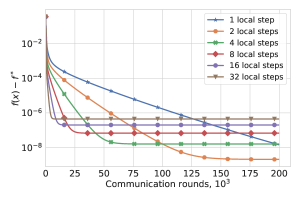
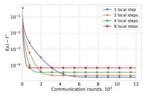
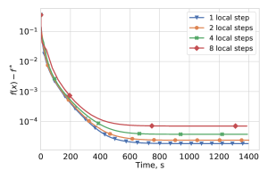
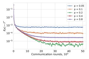
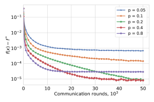
where each function is convex and -smooth. We set . We use as the stepsize, so that each is firmly nonexpansive. The results of Algorithms 1 and 2 are illustrated in Figures 1 and 3, respectively.
4.2 Local cycling GD
In this section, we consider another operator, which is cycling GD. So, we consider minimizing the same function as in (20), but this time each function is also a finite sum: . Instead of applying full gradient steps, we apply element-wise gradient steps, in the sequential order of the data points. Thus,
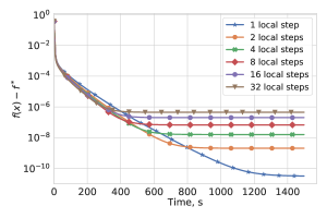
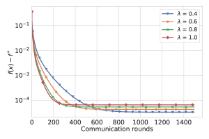
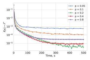
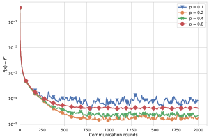
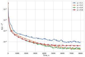
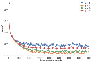
where . If, for each , all functions have the same minimizer , then this joint minimizer is a fixed point of . Also, these operators can be shown to be firmly nonexpansive. The results of Algorithms 1 and 2 are illustrated in Figures 2 and 4, respectively.
4.3 Results
We observe a very tight match between our theory and the numerical results. As can be seen, the larger the value of the parameters and , the faster the convergence at the beginning, but the larger the radius of the neighborhood. In terms of computational time, there is no big advantage, since the experiments were run on a single machine and the communication time was negligible. But in a distributed setting where communication is slow, our approach has a clear advantage. We can also observe the absence of oscillations. Hence, there is a clear advantage of local methods when only limited accuracy is required.
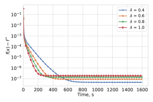
In the experiment with cyclic GD, the algorithm converges only to a neighbourhood of the ideal solution, even when 1 local step is used. This happens because the assumption of a joint minimizer for all is not satisfied here. However, since the operators are firmly nonexpansive, we have convergence to a fixed point. The convergence of Algorithm 1 is illustrated with respect to the relaxation parameter . If is small, convergence is slower, but the algorithm converges to a point closer to the true solution . In Figure 4, we further illustrate the behavior of Algorithm 2 with respect to the probability , for cyclic gradient descent. We can see that the fastest and most accurate convergence is obtained for an intermediate value of , here .
The experiments with Algorithm 2 show that, with a low probability of update, the neighborhood is substantially larger; however, with increasing, the convergence in terms of communication rounds becomes worse. Therefore, with careful selection of the probability parameter, a significant advantage can be obtained.
5 Conclusion
We have proposed two strategies to reduce the communication burden in a generic distributed setting, where a fixed point of an average of operators is sought. We have shown that they improve the convergence speed, while achieving the goal of reducing the communication load. At convergence, only an approximation of the ideal fixed point is attained, but if medium accuracy is sufficient, the proposed algorithms are particularly adequate.
In future work, we will generalize the setting to randomized fixed-point operators, to generalize stochastic gradient descent approaches. We will also investigate compression (Khaled & Richtárik, 2019; Chraibi et al., 2019) of the communicated variables, with or without variance reduction, in combination with locality.
Acknowledgements
Part of this work was done while the first author was an intern at KAUST.
References
- Bauschke & Combettes (2017) Bauschke, H. H. and Combettes, P. L. Convex Analysis and Monotone Operator Theory in Hilbert Spaces. Springer, New York, 2nd edition, 2017.
- Bauschke et al. (2011) Bauschke, H. H., Burachik, R. S., Combettes, P. L., Elser, V., Luke, D. R., and Wolkowicz, H. (eds.). Fixed-Point Algorithms for Inverse Problems in Science and Engineering. Springer, 2011.
- Chraibi et al. (2019) Chraibi, S., Khaled, A., Kovalev, D., Richtárik, P., Salim, A., and Takáč, M. Distributed fixed point methods with compressed iterates. preprint ArXiv:1912.09925, 2019.
- Combettes & Woodstock (2020) Combettes, P. L. and Woodstock, Z. C. A fixed point framework for recovering signals from nonlinear transformations. preprint arXiv:2003.01260, 2020.
- Combettes & Yamada (2015) Combettes, P. L. and Yamada, I. Compositions and convex combinations of averaged nonexpansive operators. Journal of Mathematical Analysis and Applications, 425(1):55–70, 2015.
- Davis & Yin (2016) Davis, D. and Yin, W. Convergence rate analysis of several splitting schemes. In Glowinski, R., Osher, S. J., and Yin, W. (eds.), Splitting Methods in Communication, Imaging, Science, and Engineering, pp. 115–163, Cham, 2016. Springer International Publishing.
- Haddadpour & Mahdavi (2019) Haddadpour, F. and Mahdavi, M. On the convergence of local descent methods in federated learning. preprint arXiv:1910.14425, 2019.
- Khaled & Richtárik (2019) Khaled, A. and Richtárik, P. Gradient descent with compressed iterates. In NeurIPS Workshop on Federated Learning for Data Privacy and Confidentiality, 2019.
- Khaled et al. (2019) Khaled, A., Mishchenko, K., and Richtárik, P. First analysis of local GD on heterogeneous data. In NeurIPS Workshop on Federated Learning for Data Privacy and Confidentiality, 2019.
- Khaled et al. (2020) Khaled, A., Mishchenko, K., and Richtárik, P. Tighter theory for local SGD on identical and heterogeneous data. In The 23rd International Conference on Artificial Intelligence and Statistics (AISTATS 2020), 2020.
- Konečný et al. (2016) Konečný, J., McMahan, H. B., Yu, F. X., Richtárik, P., Suresh, A. T., and Bacon, D. Federated learning: Strategies for improving communication efficiency. In NIPS Workshop on Private Multi-Party Machine Learning, 2016.
- Lessard et al. (2016) Lessard, L., Recht, B., and Packards, A. Analysis and design of optimization algorithms via integral quadratic constraints. SIAM J. Optim., 26(1):57–95, 2016.
- Ma et al. (2017) Ma, C., Konečný, J., Jaggi, M., Smith, V., Jordan, M. I., Richtárik, P., and Takáč, M. Distributed optimization with arbitrary local solvers. Optimization Methods and Software, 32(4):813–848, 2017.
- McMahan et al. (2017) McMahan, H. B., Moore, E., Ramage, D., Hampson, S., and Agüera y Arcas, B. Communication-efficient learning of deep networks from decentralized data. In Proceedings of the 20th International Conference on Artificial Intelligence and Statistics (AISTATS), 2017.
- Nesterov (2004) Nesterov, Y. Introductory lectures on convex optimization: a basic course. Kluwer Academic Publishers, 2004.
- Pesquet & Repetti (2015) Pesquet, J.-C. and Repetti, A. A class of randomized primal-dual algorithms for distributed optimization. J. Nonlinear Convex Anal., 12(16), December 2015.
- Richtárik & Takáč (2014) Richtárik, P. and Takáč, M. Iteration complexity of randomized block-coordinate descent methods for minimizing a composite function. Math. Program., 144(1–2):1–38, April 2014.
- Stich (2019) Stich, S. U. Local SGD Converges Fast and Communicates Little. In International Conference on Learning Representations, 2019.
- Yu (2013) Yu, Y.-L. On decomposing the proximal map. In Proc. of 26th Int. Conf. Neural Information Processing Systems (NIPS), pp. 91–99, 2013.
Supplementary material
Appendix A Notations and Basic Facts
A.1 Notations
Let be operators on .
Let us list here the notations used in the paper and the Appendix:
The value measures the deviation of the iterates from their average. This value is crucial for the convergence analysis. The values and can be viewed as analogues of the gradient and the average gradient in our more general setting. The value serves as a measure of variance adapted to methods with local steps.
A.2 Basic Facts
Jensen’s inequality. For any convex function and any vectors we have
| (21) |
In particular, with , we obtain
| (22) |
Facts from linear algebra.
We will use the following important properties:
| (23) |
| (24) |
| (25) |
| (26) |
Firm nonexpansiveness An operator is said to be firmly nonexpansive if it is -averaged. Equivalently, for every and ,
| (27) |
A.3 Technical lemmas
Technical Lemma 1. If is firmly nonexpansive, then
| (28) |
and
| (29) |
Proof.
We have
So,
∎
Technical Lemma 2. Let . Let be a contractive and firmly nonexpansive operator; that is, for every ,
| (30) |
Then
Proof.
We have
Since
we have
∎
Appendix B Analysis of Algorithm 1 in Theorem 2.6
The first lemma allows us to find a recursion on the optimality gap for a single step of local method:
Lemma B.1.
Under Assumption 2.5 and the condition we have, for every ,
| (31) |
Lemma B.2.
Under Assumption 2.5 and the condition we have, for every ,
| (32) |
B.1 Proof of Lemma B.1
Under Assumption 2.5 and under the condition , we have
| (33) |
B.2 Proof of Lemma B.2
B.3 Proof of Theorem 2.6
Suppose that and that Assumption 2.5 holds. Then, for every ,
| (36) |
B.4 Proof of Corollary 2.7
Suppose that and that Assumption 2.5 holds. Then a sufficient condition on the number of iterations to reach -accuracy, for any , is
| (37) |
Proof.
We have
So, we have
Using this, we get
∎
Appendix C Analysis of Algorithm 1: Proof of Theorem 2.14
We set .
First, we have
| (38) | ||||
| (39) | ||||
| (40) |
so that
| (41) |
Thus, we just have to bound :
| (42) | ||||
| (43) | ||||
| (44) | ||||
| (45) | ||||
| (46) |
Hence,
| (47) |
where
| (48) |
Appendix D Analysis of Algorithm 2
We first derive two lemmas, which will be combined to prove Theorem 3.2.
The first lemma provides a recurrence property, for one iteration of Algorithm 2:
Lemma D.1.
Under Assumption 3.1, for every ,
We now bound the variance for one iteration, using the contraction property:
Lemma D.2.
Under Assumption 3.1 and if we have, for every ,
D.1 Proof of Lemma D.1
Under Assumption 3.1, for every and , we have
| (49) |
D.2 Proof of Lemma D.2
Under Assumption 3.1 and if , we have, for every ,
| (51) |
Proof.
If communication happens, . Therefore,
Using Young’s inequality (25),
Using our notations,
Applying the same technique, we get:
Setting , , we get
By averaging,
Using this inequality,
Finally, we get
∎
D.3 Proof of Theorem 3.2
For every , let be the Lyapunov function defined as:
| (52) |
Under Assumption 3.1 and if , we have, for every ,
| (53) |
D.4 Proof of Corollary 3.3
Under Assumption 3.1 and if , for any , -accuracy is reached after iterations, with
| (54) |
Proof.
We start from
Regarding the second term, if , then ,
so that
Regarding the first term, and using the fact that , if ,
then , so that
Finally, we get
∎