Long-term prediction of chaotic systems with recurrent neural networks

Abstract

Reservoir computing systems, a class of recurrent neural networks, have recently been exploited for model-free, data-based prediction of the state evolution of a variety of chaotic dynamical systems. The prediction horizon demonstrated has been about half dozen Lyapunov time. Is it possible to significantly extend the prediction time beyond what has been achieved so far? We articulate a scheme incorporating time-dependent but sparse data inputs into reservoir computing and demonstrate that such rare “updates” of the actual state practically enable an arbitrarily long prediction horizon for a variety of chaotic systems. A physical understanding based on the theory of temporal synchronization is developed.

A recently emerged interdisciplinary field is machine-learning based, model-free prediction of the state evolution of nonlinear/chaotic dynamical systems Haynes et al. (2015); Larger et al. (2017); Pathak et al. (2017); Lu et al. (2017); Duriez et al. (2017); Pathak et al. (2018a, b); Carroll (2018); Nakai and Saiki (2018); Roland and Parlitz (2018); Weng et al. (2019); Jiang and Lai (2019). A paradigm that has been exploited is reservoir computing Jaeger (2001); Mass et al. (2002); Jaeger and Haas (2004); Manjunath and Jaeger (2013), a class of recurrent neural networks. Starting from the same initial condition, a well-trained reservoir system can generate a trajectory that stays close to that of the target system for a finite amount of time, realizing short-term prediction. Because of the hallmark of chaos - sensitive dependence on initial conditions, the solution of the reservoir system will diverge from that of the original system exponentially. Nonetheless, if training is done properly so that the single-step error is orders-of-magnitude smaller than the oscillation range of the chaotic signal Jiang and Lai (2019), accurate prediction can be achieved in short time. So far, the prediction horizon achieved is about five or six Lyapunov time Pathak et al. (2018b), where one Lyapunov time is the inverse of the maximum Lyapunov exponent.

Is it possible to extend significantly the prediction horizon of reservoir computing? We provide an affirmative answer in this paper. The key observation is that, after training, prediction is enabled because the neural network system can replicate the dynamical evolution of the target system (or synchronize with it) but only for a transient period of time. In the conventional scheme, data from the target system are used only during the training phase. A solution to extend the transient time is to provide some “update” of the target system. We thus conceive the scenario where, after the initial training, infrequent or sparse updates in the form of new measurement or observation of the target system are available. We demonstrate that even rare updates of the actual state enable an arbitrarily long prediction horizon to be achieved for a variety of chaotic systems. Essentially, before the trajectories of the reservoir and original systems diverge substantially (e.g., about to exceed a predefined accuracy), we correct the state of the reservoir system with real measurement of duration as few as a single data point. We develop a physical understanding based on the theory of temporal synchronization. Practically, with rare data updates, the reservoir computing system can replicate the evolution of the original system within some desired accuracy for an arbitrarily long time, in spite of chaos. This will have applications in fields where chaos arises.

Figure 1: Proposed reservoir computing (RC) system with rare state updates in the prediction phase, which is capable of generating arbitrarily long prediction of the state evolution of any chaotic system. The I/R, Reservoir, and R/O modules within the blue dashed box constitute the conventional reservoir computing system. Initial training with data from the target chaotic system is done in a conventional manner. The articulated scheme of rare state updates is represented by the C/I module inside the red dashed box, which couples sparse measurement data with the output of the system to generate updated inputs to the system.

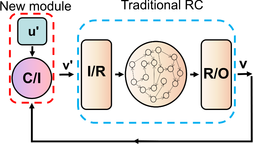
The basic working of reservoir computing can be described briefly as follows. Suppose time series data represented by a relatively low-dimensional data vector from the target system to be predicted are available. As shown in Fig. 1, one feeds the time series into the input-to-reservoir (I/R) module to generate a time-dependent data vector whose dimension is significantly larger than that of the original data vector. The high-dimensional vector is then sent to a complex network constituting the core of the reservoir, whose size matches the dimension of the vector. That is, there is a one-to-one correspondence between any component of the high-dimensional vector and a node in the network, and the data from a component is fed into the corresponding node. The state of the reservoir network is updated according to some nonlinear function, and the resulting state vector is sent to a reservoir-to-output (R/O) module whose function is opposite to that of the I/R module, i.e., to convert the high-dimensional vector of the reservoir back into a vector of the same low-dimension as that of the original data from the target system. The reservoir network, once chosen, is fixed, so all parameters associated with it are hyperparameters. Training is done through a relatively small set of adjustable parameters associated with the R/O module, which can be tuned (or “learned”) based on the available input data. During the training phase, the system is open as it requires input from the target system. After training, one feeds the output from R/O directly into the I/R module, closing the system. The system then evolves by itself. Some key numbers involved in reservoir computing for model-free prediction are as follows. For example, for the Kuramoto-Sivashinsky equation (KSE) with spatiotemporally chaotic solutions Pathak et al. (2018b), the typical number of the spatial measurement sites (the dimension of the input vector) is 64 and the size of the reservoir network is about 5000. The number of parameters in the R/O module to be trained is $5000\times 64$.

Our proposed reservoir computing system functioning in the prediction phase leading to arbitrarily long prediction horizon is shown schematically in Fig. 1, where the three modules inside the blue dashed box represent the conventional system and the one inside the red dashed box is a new module incorporating rare state updates. The $I/R$ module is described by $\bm{W}_{in}$, a $D_{r}\times D_{in}$ random matrix that maps a $D_{in}$-dimensional input vector $\bm{v}$ into a $D_{r}$-dimensional vector $\bm{r}(t)$, where $D_{in}\ll D_{r}$. The elements of $\bm{W}_{in}$ are generated from a uniform distribution in $[-\sigma,\sigma]$. The reservoir is a complex network of $D_{r}$ nodes with average degree $d$, whose connecting topology is described by the $D_{r}\times D_{r}$ matrix $\bm{A}$. (For simplicity, we choose it to be a directed random network.) A recent work Jiang and Lai (2019) has revealed that successful training and finite-time prediction can be achieved if the spectral radius of the network is in a finite range, which can be adjusted by properly normalizing the link weights in the network. The $R/I$ module is represented by a $D_{out}\times D_{r}$ matrix, whose elements are parameters determined through training Pathak et al. (2017, 2018b). Typically, we have $D_{out}=D_{in}$. Without any state update, in the prediction phase, the reservoir computing system is a self-evolving dynamical system described by $\bm{r}(t+\Delta t)=\tanh{[\bm{A}\cdot\bm{r}(t)+\bm{W}_{in}\cdot\bm{v}(t)]}$ and $\bm{v}(t+\Delta t)=\bm{W}_{out}\cdot\bm{f}[\bm{r}(t+\Delta t)]$, where $\bm{f}(\bm{r})$ is the output function Pathak et al. (2017, 2018b): $f_{i}(\bm{r})=r_{i}$ and $f_{i}(\bm{r})=r^{2}_{i}$ for odd and even index $i$, ($i=1,2,\ldots,D_{r}$), respectively. Associated with the dynamical evolution of the reservoir system are two sets of dynamical variables: the high-dimensional reservoir state vector $\bm{r}$ and the (typically) low-dimensional output vector $\bm{v}$. The matrices $\bm{W}_{in}$ and $\bm{A}$ are pre-defined while $\bm{W}_{out}$ is determined by training during which $\bm{v}$ is replaced by the state vector $\bm{u}$ of the target system. After training is completed, to set the initial condition for the reservoir network, one approach is to continue to use $\bm{u}$ in place of $\bm{v}$ but only for a few time steps, after which the reservoir system executes natural dynamical evolution by itself.

In the conventional scheme Haynes et al. (2015); Larger et al. (2017); Pathak et al. (2017); Lu et al. (2017); Duriez et al. (2017); Pathak et al. (2018a, b); Carroll (2018); Nakai and Saiki (2018); Roland and Parlitz (2018); Weng et al. (2019); Jiang and Lai (2019), after withdrawing the true state vector $\bm{u}$ so that the system is closed, real measurements are no longer used, resulting in a relatively short prediction horizon for chaotic systems because of the exponential divergence between the trajectories of the reservoir and true systems. Our idea, as shown in Fig. 1, is to update the reservoir state with sparsely sampled real state vector $\bm{u}^{\prime}$ before the divergence exceeds a pre-defined tolerance limit, i.e., the updates are needed only rarely. In particular, during the update, the input to the I/R module can be written as $\bm{v}^{\prime}(t)=\bm{v}(t)+c[\bm{u}^{\prime}(t)-\bm{v}(t)]$, where $\bm{u}^{\prime}$ contains data at $t$ and $c$ is the coupling parameter. Most of the time during the evolution, we still have $\bm{v}^{\prime}(t)=\bm{v}(t)$. Updating is effectively an on-off coupling process between the reservoir and the true systems, where the “on” phase is significantly more sparse than the “off” phase. Prediction can then be viewed as a synchronization process Lu et al. (2018); Weng et al. (2019) between the two systems that are coupled but only intermittently Chen et al. (2009); Li et al. (2018).

We test the predictive power of our proposed reservoir computing scheme with a large number of chaotic systems. Here we present two examples of high-dimensional chaotic systems: KSE and the complex Ginzburg-Landau equation (cGLE). (Examples of a number of low-dimensional chaotic systems are presented in Appendices.) The KSE is $y_{t}+yy_{x}+y_{xx}+y_{xxxx}=0$, where $y(x,t)$ is a scalar field in the interval $x\in(0,L)$ with periodic boundaries. We divide the spatial domain into $M$ uniform subintervals. Figure 2(a) shows a typical spatiotemporal chaotic solution for $L=22$, where the numerical integration parameters are $M=64$ and $\Delta t=0.25$, and the maximum Lyapunov exponent is $\Lambda_{max}\approx 0.05$. Thus, approximately 80 time steps correspond to one Lyapunov time. The $M$-dimensional data vector is fed into the reservoir computing system with parameters $D_{in}=D_{out}=M$, $D_{r}=4992$, $\sigma=1$, $d=3$, and $\rho=0.1$. In addition, to avoid overfitting of $\bm{W}_{out}$ during the training process, we set the relevant bias parameter Pathak et al. (2018b) to be $\eta=1\times 10^{-4}$. Figure 2(b) shows the difference between the evolution of the reservoir and true system, i.e., the prediction error (color coded). The prediction horizon is about five Lyapunov time.

Figure 2: Prediction of spatiotemporal chaotic solution of KSE. The system size is $L=22$, the number of measurement points is $M=64$, and the value of the coupling parameter is $c=1.0$. (a) True spatiotemporal evolution of the chaotic solution. (b) The difference (error) between the predicted and true solutions without any measurement updating, i.e., with updating period $T=\infty$. The prediction horizon is about five Lyapunov time. (c-e) The error with updating period $T=240$, 160, and 80 time steps, corresponding to three, two, and one Lyapunov time, respectively, where the update consists of a single date point from the true system. In (e), error at all time is below the tolerance, signifying an arbitrarily long prediction horizon.

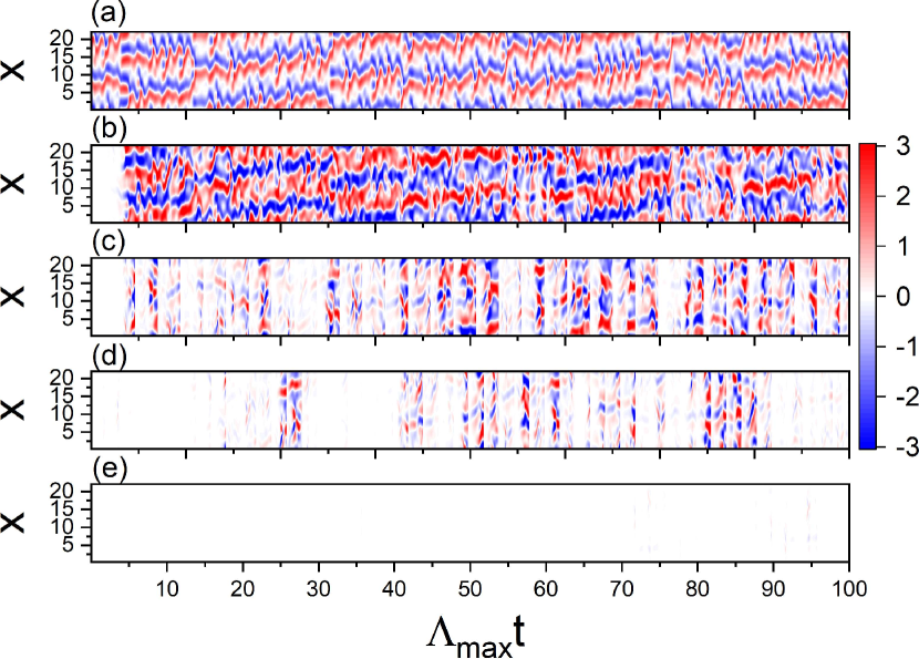
We now instigate rare updates with the true data $y_{act}(x,t)$, where the coupling function is $y_{rc}^{\prime}(x,t)=y_{rc}(x,t)+c[y_{act}(x,t)-y_{rc}(x,t)]$ if there is data update at the space-time point $(x,t)$, otherwise we have $y_{rc}^{\prime}(x,t)=y_{rc}(x,t)$, where $y_{rc}$ is the output of the reservoir system. We divide the output time series into equal time intervals, each of $T$ time steps. In one interval, the actual data points are available for consecutive $T_{0}$ steps, and there is no update for the remaining $T-T_{0}$ steps. In the space, we select $M_{c}$ uniform spatial points from the total $M$ measurement points. For illustration, we $T_{0}=1$ and $M_{c}=64$, i.e., each component of the input vector to the reservoir system (corresponding to a distinct measurement point in space) receives one true data point every $T$ time steps. Figure 2(c-e) show the prediction error for $T=240$, 160, and 80 time steps, respectively, corresponding to three, two, and one Lyapunov time. For $T=240$ [Fig. 2(c)], the error is reduced as compared the case of no data update [Fig. 2(b)] and exhibits intermittency, implying an intermittently synchronous behavior between the reservoir and the true system. In this case, the time interval in which the error is below the tolerance emerges intermittently in time. As the updating becomes twice as frequent, the small-error intervals are generally enlarged, as shown in Fig. 2(d) for $T=160$. Remarkable, for $T=80$, the error is essentially zero in the whole time interval considered. This means that, insofar as a single true data point is used to update the reservoir system in every Lyapunov time, the prediction horizon becomes arbitrarily long!

Figure 3: Behaviors of prediction error for KSE. (a) Prediction error in the parameter plane $(T_{0},T)$ for $M_{c}=32$ and $c=2.0$. (b) For $M_{c}=32$, prediction error $\delta e$ versus $T$ for different values of $T_{0}$. (c) Prediction error for $M_{c}=64$ and $c=1.0$. (d) For $M_{c}=64$, $\delta e$ versus $T$ for different values of $T_{0}$. (e) For random updating, prediction error in the parameter plane $(p_{t},p_{s})$ for $c=1.2$ and (f) $\delta e$ versus $p_{t}$ (or $T_{0}/T$).

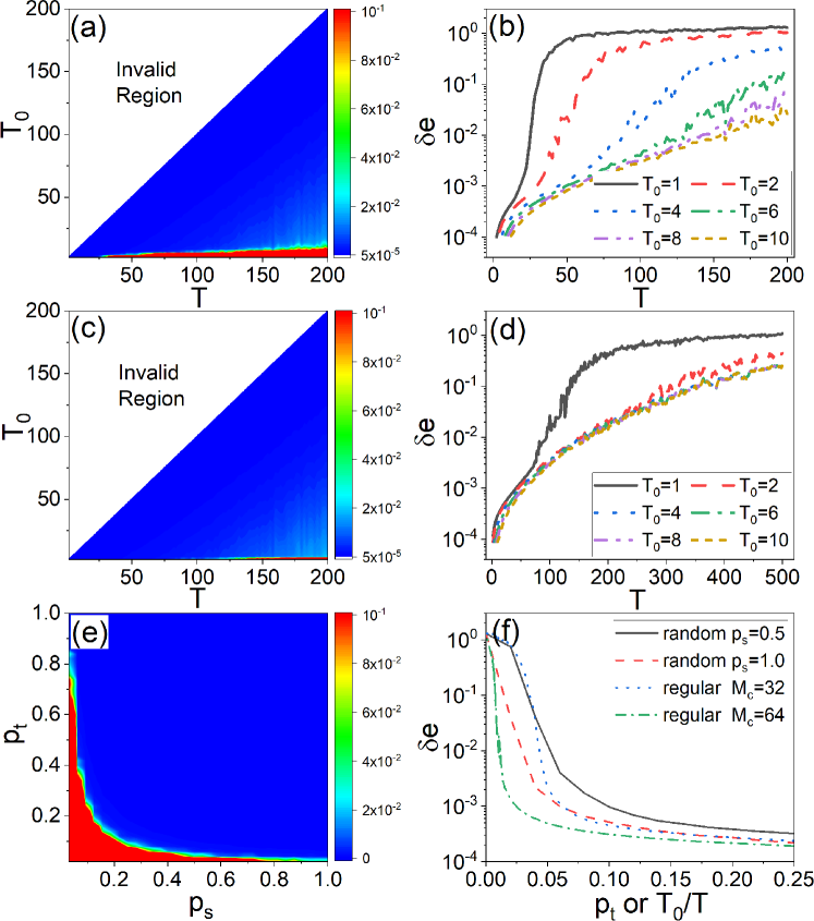
To obtain a systematic picture of the prediction horizon, we calculate the average error $\delta e$ over a long time interval, e.g., about 100 Lyapunov time, in the parameter plane $(T_{0},T)$ (for $T_{0}\leq T$). Figure 3(a) shows, for $M_{c}=M/2=32$ (the number of spatial coupling channels) and $c=2.0$, the error behavior. In most of the parameter region, the error is small: $\delta e<0.01$. Long term prediction fails only for extremely rare updates, i.e., for small values of $T_{0}$ and large values of $T$. Fixing the value of $T_{0}$, we obtain the curves of $\delta e$ versus $T$. For $T_{0}=1$ (black line), $\delta e$ increases rapidly with $T$. As more data points are included in each update, e.g., as the value of $T_{0}$ is increased from two to ten, $\delta e$ decreases gradually. Figure 3(c) shows that, for $M_{c}=M=64$, the error remains small in all cases, giving rise to a significantly augmented prediction horizon. Figure 3(d) shows the prediction error for $T$ up to $500$ time steps. For a change from $T_{0}=1$ to $T_{0}=2$, error $\delta e$ decreases sharply. However, for $T_{0}\geq 2$, the predictions error becomes saturated. Comparing Figs. 3(b) with 3(d), we observe a dramatic reduction in $\delta e$ for $M_{c}=64$.

The cases considered so far are for rare but regular updates. What about random updates? We examine the parameter plane $(p_{t},p_{s})$, where $p_{t}$ is the probability of update in each time step and $p_{s}$ is the probability for a spatial point to receive updates. Figure 3(e) shows the average prediction error, which exhibits an approximately symmetric behavior with respect to $p_{t}$ and $p_{s}$. Figure 3(f) shows, for fixed $p_{s}=0.5$ and $p_{s}=1$ (corresponding to the cases of $M_{c}=32$ and $M_{c}=64$ with regular coupling, respectively), random updating yields somewhat larger errors than those with regular coupling.

Figure 4: Long time prediction of the state evolution of one-dimensional cGLE and . The system size is $L=18$ and the number of measurement sites is $M=32$. (a) Spatiotemporal pattern of true state evolution. (b-e) The difference between the predicted and actual state evolution for $T=\infty$, $T=195$, $T=130$, and $T=65$, respectively. (f) For regular updating, prediction error in the parameter plane $(T_{0},T)$ for $M_{c}=32$ and $c=0.4$. (g) For random updating, prediction error in the parameter plane $(p_{t},p_{s})$ for $c=0.4$.

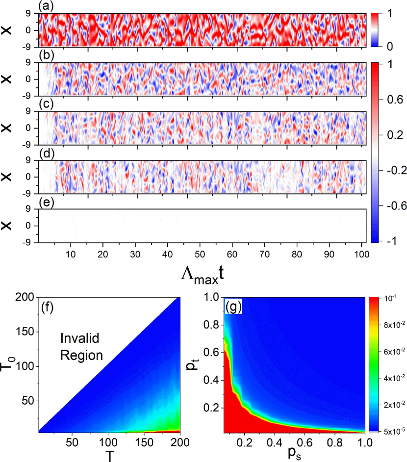
We now demonstrate the predictive power of our reservoir computing scheme for the 1D cGLE in the regime of spatiotemporal chaos: $A_{t}=(1+i\alpha)A_{xx}+A-(1+i\beta)|A|^{2}A$, where $A(x,t)$ is a complex field in the interval $x\in(-L/2,L/2)$ with the periodic boundary condition, $\alpha$ and $\beta$ are parameters. The cGLE is a general model for a variety of physical phenomena Aranson and Kramer (2002); Cross and Hohenberg (1993); Kuramoto (1984). For $L=18$, $\alpha=2$ and $\beta=-2$, the 1D cGLE exhibits spatiotemporal chaos with the maximum Lyapunov exponent $\Lambda\approx 0.23$. We divide the whole interval into $M=32$ equally spaced points - the measurement sites. For integration step $\Delta t=0.07$, one Lyapunov time corresponds to about 65 time steps. Figure 4(a) shows the true spatiotemporal evolution pattern $|A(x,t)|$. Because the field $A(x,t)$ is complex, it is necessary to use both the real [$A^{r}(x,t)$] and imaginary [$A^{i}(x,t)$] parts for training the reservoir system. The parameters of the reservoir system are $D_{in}=D_{out}=2M$, $D_{r}=9984$, $\sigma=1$, $d=3$, $\rho=0.1$, and $\eta=2\times 10^{-5}$. Without any update, the error between the predicted and true state evolution is shown in Fig. 4(b), where the prediction horizon is about five Lyapunov time. To introduce rare updates of the true state, we use the coupling scheme $A^{\prime r(i)}_{rc}(x,t)=A^{r(i)}_{rc}(x,t)+0.4[A^{r(i)}_{act}(x,t)-A^{r(i)}_{rc}(x,t)]$ if there is actual data at the space-time point $(x,t)$, and otherwise $A^{\prime r(i)}_{rc}(x,t)=A^{r(i)}_{rc}(x,t)$, where $A^{r(i)}_{act}(x,t)$ is the real (imaginary) part of the true data and $A^{r(i)}_{rc}$ is the real (imaginary) part of predicted state. We demonstrate updating with only a single data point: $T_{0}=1$. Figures 4(c-e) show the prediction error for $T=195$, 130, and 65, corresponding to three, two, and one Lyapunov time, respectively. Evidence of intermittent synchronization between the reservoir and the actual systems is shown in Figs. 4(c) and 4(d). As for the spatiotemporally chaotic KSE system, updating the reservoir system with a single data point every Lyapunov time [Fig. 4(e)] leads to arbitrarily long prediction horizon for the spatiotemporally chaotic state of the 1D cGLE.

Figures 4(f) and 4(g) show the time averaged prediction error $\delta e$ in the parameter planes $(T_{0},T)$ (regular updating scheme) and $(p_{s},p_{t})$ (random updating scheme), respectively, where the average is taken over approximately 100 Lyapunov time. For regular updating, small prediction error can be achieved in most of the parameter plane. For random updating, the error decreases with an increase in $p_{t}$ and/or $p_{s}$.

The theoretical explanation for the observed long-term prediction is that, after proper training the output vector of the reservoir system follows the state vector of the target system for a finite amount of time, indicating complete synchronization between the two systems. Without state updating, the synchronization state is slightly unstable, leading to a short prediction horizon. State updates, even applied rarely, represent a kind of perturbation that makes the synchronization state less unstable, prolonging the prediction horizon. When the frequency of the updates is such that there is one update within one Lyapunov time, the synchronization state becomes stable, giving rise to an arbitrarily long prediction horizon. This scenario has been verified using low-dimensional chaotic systems (Appendix A) through a synchronization stability analysis Heagy et al. (1995); Pecora and Carroll (1998). We also note that, for a variety of low-dimensional chaotic systems including the classic Rössler Rössler (1976) and Lorenz Lorenz (1963) oscillators, the Hindmarsh-Rose neuron Hindmarsh and Rose (1984), and a chaotic food web Blasius et al. (1999), rare updates to a single state variable enables a properly trained reservoir system to predict all state variables for an arbitrarily long period of time (Appendices B-D). For example, for the chaotic food web, it is necessary only to supply sparse vegetation data for the reservoir system to correctly predict the abundances of the herbivores and predators, for as long as one wishes.

To summarize, existing reservoir computing systems can predict the dynamical evolution of chaotic systems but only for a short period of time. We have articulated a scheme incorporating true state updates and demonstrated that rare updates of a subset of state variables can significantly prolong the prediction horizon. Of particular interest is the finding that, insofar as there is state update of a single data point within one Lyapunov time, the prediction horizon can be made arbitrarily long. The machine learning scheme proposed and studied here has the potential to extend significantly the application scope of reservoir computing in predicting complex dynamical systems.

The novelty of our work is threefold: (1) we have introduced intermittent data updates into machine learning, (2) we have demonstrated that long prediction time can be achieved, and (3) we have introduced the concept of temporal synchronization with on-off coupling to understand the working of the reservoir computing machine with state updating. Our work sheds new light in the working of reservoir computing in predicting the state evolution of chaotic systems. In particular, in the synchronization-based scenario, the predictability of reservoir computing is the result of its ability to synchronize with the target chaotic system for a finite amount of time. At the start of the prediction phase, the reservoir system has the same initial condition as the target system. Because of temporal synchronizability, the reservoir system is able to follow the target system for sometime before the synchronization error becomes significant. Without state updates, the time it takes for the error to grow to a predefined threshold value determines the prediction time. State updates, even being rare, reset the synchronization error from time to time, insofar as a new update is provided before the error exceeds the threshold.

In essence, the basic idea of our method is similar to that of data assimilation, where models and measurements (true state updates) are combined to generate accurate predictions with applications in, e.g., weather forecasting Patil et al. (2001); Ott et al. (2004); Szunyogh et al. (2005). In a recent study, data assimilation and machine learning have been combined to emulate the Lorenz 96 model from sparse and noisy observations Brajard et al. (2019). It is also noteworthy that, in predicting chaotic dynamical systems, an alternative machine-learning based framework is radial basis function networks - artificial neural networks employing radial basis functions as activation functions Broomhead and Lowe (1988); Poggio and Girosi (1990). Given a set of inputs, such a network outputs a signal that is a linear combination of radial basis functions of the inputs, and the parameters of the artificial neurons are determined through training based on, e.g., the standard backpropagation scheme. The method has been demonstrated to be effective for low-dimensional chaotic systems such as the logistic map and the classic Lorenz chaotic oscillator Gholipour et al. (2006); Chen and Han (2013); Rafsanjani and Samareh (2016); Nguyen and Duong (2018). Whether the method can be superior to reservoir computing in predicting spatiotemporal chaotic systems is an open question.

Appendix A Mechanism for reservoir computing to achieve arbitrarily long prediction horizon - a heuristic analysis based on synchronization

To understand the mechanism behind the realization of long prediction horizon in our proposed reservoir computing scheme with state updating, we resort to synchronization analysis. To facilitate the analysis, we apply our scheme to the chaotic Rössler oscillator given by Rössler (1976):

$$\dot{x}=-y-z,$$

$$\dot{y}=x+0.2y,$$ (1)

$$\dot{z}=0.2+(x-9.0)z.$$

We obtain the three time series [$x(t)$, $y(t)$, $z(t)$] at the step size $\Delta t=0.05$. The values of the parameters of the reservoir computing system are $D_{in}=D_{out}=3$, $D_{r}=600$, $\sigma=0.15$, $d^{\prime}=0.2$, $\rho=0.2$, and $\eta=1\times 10^{-7}$, where $d^{\prime}$ is the link density of the complex neural network. The elements of the $D_{r}\times D_{in}$ input matrix $\bm{W}_{in}$ are generated from the uniform distribution $[-\sigma,\sigma]$. The non-zero elements of the $D_{r}\times D_{r}$ matrix $\bm{A}$ are generated from the uniform distribution $[-1,1]$. Figure 5(a) shows the prediction result with the conventional scheme, where the prediction horizon is about $t\approx 75$ (corresponding to approximately 15 average cycles of oscillation). Figure 5(b) shows that, with our proposed scheme, the prediction horizon is practically infinite, where an update of the actual data of a single dynamical variable, $y_{act}$, is coupled into the system ($T_{0}=1$ and $T=50$) once every 50 time steps. More specifically, in the iterative process of reservoir computing system, the input data $y_{rc}$ is replaced by $y^{\prime}_{rc}=y_{rc}+c(y_{act}-y_{rc})$ once every 50 time steps for $c=0.8$. Note that, in Fig. 5(b), only the true and predicted $x$ time series are shown, but time series from the other two dynamical variables give essentially the same prediction result. Figure 5(c) shows the color-coded average prediction error $\delta e$ in the parameter plane $(T_{0},T)$, where there are multiple parameter regions in which the error is small. The patterns in Fig. 5(c) are reminiscent of the phenomenon of ragged synchronization in coupled chaotic oscillator systems Stefański et al. (2007); Perlikowski et al. (2008), suggesting the use of synchronization theory to understand the working mechanism of our articulated reservoir computing machine.

Figure 5: Predicting state evolution of chaotic Rössler oscillator and synchronization analysis. (a) Result of prediction with conventional reservoir computing: true (black) and predicted (red) time series $x(t)$. The prediction horizon is approximately 15 average periods of oscillation as the true and predicted time series begin to diverge after this time. (b) True and predicted time series with our proposed reservoir computing scheme incorporating rare state updating. The two time series overlap completely and the prediction horizon is practically infinite. (c) Color-coded prediction error in the parameter plane $(T_{0},T)$, where $T$ is the updating period (in units of $\Delta t$, the time step between two successive iterations of the reservoir neural network) and $T_{0}<T$ is the number of time steps during which there is true data input. (d) The maximum transverse Lyapunov exponent in $(T_{0},T)$ from synchronization analysis. There is a qualitative correspondence between the small error [(c)] and negative Lyapunov exponent regions in the parameter plane.

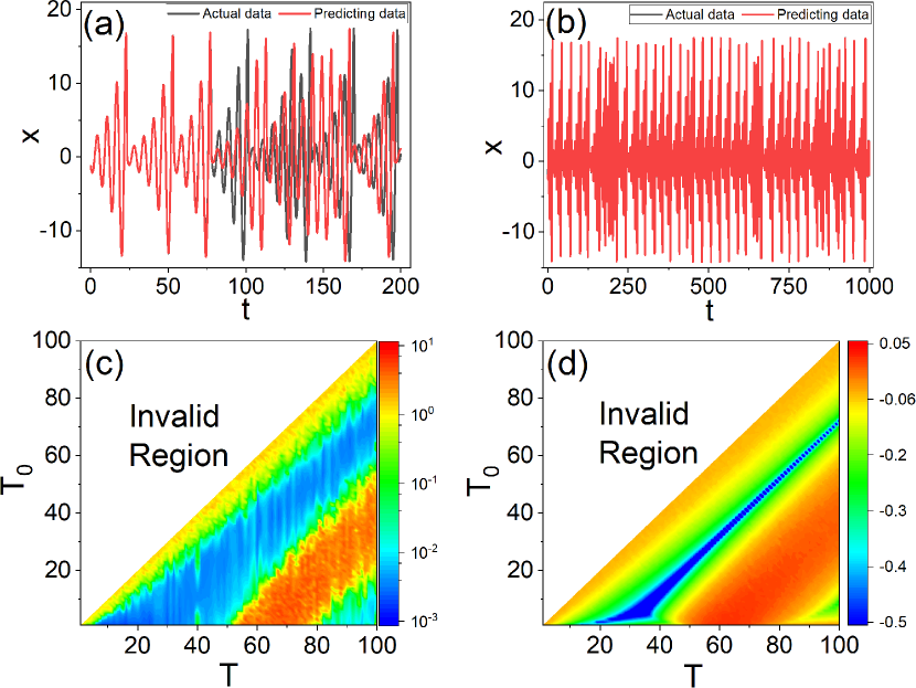
A well trained reservoir computing system can be viewed as a high-dimensional replica of the target system. A previous calculation of the Lyapunov exponents of the reservoir dynamical network revealed that the first few exponents are indeed approximate values of the exponents of the true system, and the vast set of remaining exponents have large negative values Pathak et al. (2017). This is anticipated as the large negative exponents are necessary to reduce the exceedingly high dimension of the reservoir network to the low-dimensional target system through a strong compression of the dynamics along vast majority of orthogonal directions in the phase space. For the chaotic Rössler system, the considerations suggest that the dynamics of the reservoir computing system be approximately described by

$$\dot{x}_{rc}=-y_{rc}-z_{rc},$$ (2)

$$\dot{y}_{rc}=x_{rc}+0.2y_{rc}+\varepsilon(t)(y_{act}-y_{rc}),$$

$$\dot{z}_{rc}=0.2+(x_{rc}-9)z_{rc},$$

where, in the coupling term $\varepsilon(t)(y_{act}-y_{rc})$, $\varepsilon(t)$ specifies the on-off nature of the coupling: $\varepsilon(t)=\varepsilon$ if $nT\Delta t<t<T_{0}\Delta t+nT\Delta t$ ($n=0,1,2,\ldots$) and $\varepsilon(t)=0$ otherwise. There is a linear relation between $\varepsilon$ and $c$: $c=\varepsilon\Delta t$. The data of $y_{act}$ are generated from the target system Eq. (A). In our scheme, predictability implies synchronization between the reduced reservoir computing system Eq. (2) and the true system Eq. (A) with only on-off coupling, where the “on” phase is typically significantly shorter than the “off” phase.

We use stability analysis to quantify synchronization. Let $\delta x=x_{rc}-x_{act}$, $\delta y=y_{rc}-y_{act}$, and $\delta z=z_{rc}-z_{act}$ be the infinitesimal perturbations transverse to the synchronization manifold. The variational equations can be obtained by linearizing Eq. (2) with respect to the true state of the target system as described by Eq. (A):

$$\delta\dot{x}=-\delta y-\delta z,$$

$$\delta\dot{y}=\delta x+0.2\delta y-\varepsilon(t)\delta y,$$ (3)

$$\delta\dot{z}=z\delta x+(x-9.0)\delta z.$$

Combining Eqs. (A) and (A), we calculate the maximum transverse Lyapunov exponent $\Lambda$. Stable synchronization requires $\Lambda<0$. Figure 5(d) shows the color-coded value of $\Lambda$ in the parameter plane $(T_{0},T)$, which exhibits typical features of ragged synchronization Stefański et al. (2007); Perlikowski et al. (2008). Comparing Fig. 5(c) with Fig. 5(d), we observe a striking degree of similarity, indicating synchronization between the reservoir computing and the target systems subject to on-off coupling as the dynamical mechanism responsible for realizing the long prediction horizon with rare data updating.

Figure 6: Predicting the chaotic Lorenz system with rare state updating. (a) Prediction with the conventional reservoir computing scheme without state updating, where the prediction horizon is about ten oscillations. (b) Practically infinite prediction horizon achieved with sparse input of actual data for $T_{0}=1$, $T=40$, and $c=0.8$. (c,d) The difference between the prediction and actual time series corresponding to the results in (a,b), respectively.

Appendix B Predicting chaotic Lorenz system

We demonstrate that a practically infinite prediction horizon can be achieved for the classic chaotic Lorenz system Lorenz (1963) with rare state updating. The equations of the system are

$$\dot{x}=10(y-x),$$

$$\dot{y}=x(28-z)-y,$$ (4)

$$\dot{z}=xy-8/3z.$$

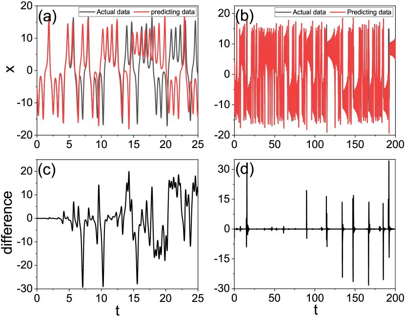
We obtain the time series $x(t)$, $y(t)$, and $z(t)$ with integration step size $\Delta t=0.01$. The parameter setting of the reservoir computing system is $D_{in}=D_{out}=3$, $D_{r}=600$, $\sigma=0.1$, $d^{\prime}=0.3$, $\rho=1.2$, and $\eta=1\times 10^{-5}$. Figure 6(a) shows the prediction result with the conventional scheme without any state updating, where the prediction horizon is $t\approx 5$ (corresponding to approximately ten average oscillations). Figure 6(b) shows that, with rare state updating ($T_{0}=1$ and $T=40$) of one of the dynamical variables, mathematically represented as replacement of $y_{rc}$ by $y^{\prime}_{rc}=y_{rc}+c(y_{act}-y_{rc})$ once every 40 time steps, practically an arbitrarily long prediction horizon can be achieved. Figures 6(c) and 6(d) show the difference between the predicted and true time series from the conventional and our proposed reservoir computing schemes, respectively. It can be seen that, with rare state updating, the prediction error is essentially zero for the time interval displayed, with relatively large errors occurring only at about a few dozen time steps (out of $2\times 10^{4}$ time steps).

Figure 7: Predicting the state evolution of a chaotic Hindmarsh-Rose neuron. (a) Prediction without state updating. (b) Arbitrarily long prediction horizon with rare state updating for $T_{0}=1$, $T=300$, and $c=0.9$. (c,d) The difference between the predicted and true state evolution for the cases in (a,b), respectively.

Figure 8: Predicting the state evolution of the populations of a chaotic food web. (a) Predicted and actual state evolution with the conventional reservoir computing scheme without any state updating. (b) Prediction result with rate state updating: once every 50 time steps ($T_{0}=1$ and $T=50$). The value of the coupling parameter is $c=1$. (c,d) Evolution of the prediction error corresponding to the cases in (a,b), respectively. With the rare state updating, the prediction error is practically zero in the entire time interval of $10^{4}$ time steps tested.

Appendix C Predicting chaotic Hindmarsh-Rose neuron dynamics

We test our reservoir computing scheme with rare state updating for the chaotic Hindmarsh-Rose neuron model Hindmarsh and Rose (1984):

$$\dot{x}=y+3x^{2}-x^{3}-z+3.2,$$

$$\dot{y}=1-5x^{2}-y,$$ (5)

$$\dot{z}=-0.006z+0.024(x+1.6),$$

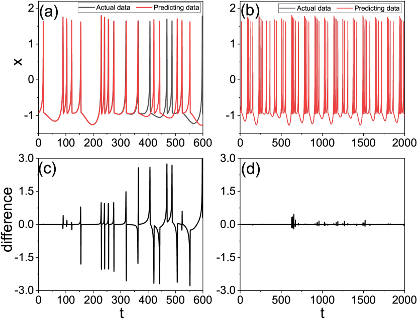
where $x$ is the membrane potential, $y$ and $z$ are the transport rates of the fast and slow channels, respectively. The integration time step is $\Delta t=0.1$. The three time series $x(t)$, $y(t)$, and $z(t)$ are used to train the reservoir computing system with parameters $D_{in}=D_{out}=3$, $D_{r}=600$, $\sigma=0.6$, $d^{\prime}=0.2$, $\rho=0.3$, and $\eta=1\times 10^{-7}$. Figure 7(a) shows the result with the conventional reservoir computing scheme without any state updating, where the prediction horizon is $t\approx 300$, in which there are about a dozen spiking events. With rare state updating (once every 100 time steps: $T_{0}=1$ and $T=100$) of two state variables ($x_{act}$ and $y_{act}$), the prediction horizon is practically infinite. Mathematically, the updating scheme can be described as a single replacement every 100 time steps of $x_{rc}$ and $y_{rc}$ by $x^{\prime}_{rc}=x_{rc}+c(x_{act}-x_{rc})$ and $y^{\prime}_{rc}=y_{rc}+c(y_{act}-y_{rc})$ respectively, for $c=0.9$. The prediction errors corresponding to Figs. 7(a) and 7(b) are shown in Figs. 7(c) and 7(d), respectively.

Appendix D Predicting population evolution in a chaotic food web

We demonstrate an arbitrarily long prediction horizon for the following chaotic food web system Blasius et al. (1999):

$$\dot{x}=x-0.2\frac{xy}{1+0.05x},$$

$$\dot{y}=-y+0.2\frac{xy}{1+0.05x}-yz,$$ (6)

$$\dot{z}=-10(z-0.006)+yz,$$

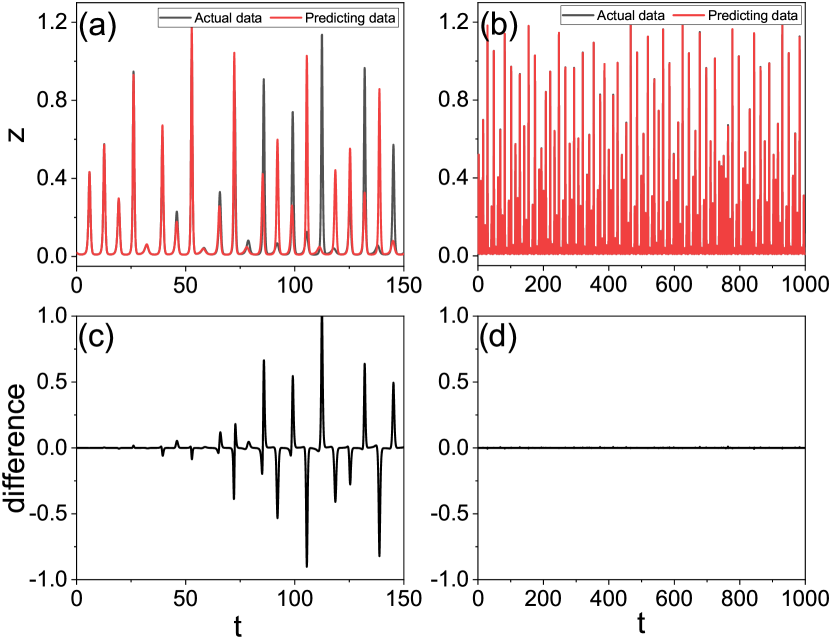
where $x$, $y$ and $z$ represent vegetation, herbivores and predators, and the evolution displays uniform phase evolution but with chaotic amplitude modulation. The integration step size is $\Delta t=0.1$. The parameter values of the reservoir computing system are $D_{in}=D_{out}=3$, $D_{r}=600$, $\sigma=0.15$, $d^{\prime}=0.2$, $\rho=0.2$, and $\eta=1\times 10^{-7}$. Figure 8(a) shows the prediction result from the conventional scheme without any state updating, where the prediction horizon is $t\approx 50$ (containing seven or eight bursts in the predator population). In the food web system, vegetation data are relatively easy to be collected, so we use $x_{act}$ to perform rare state updating. Figure 8(b) shows the predicted and actual predator time series for $T_{0}=1$ and $T=50$, i.e., we replace $x_{rc}$ by $x^{\prime}_{rc}=x_{rc}+c(x_{act}-x_{rc})$ once every 50 time steps. Visually the two types of time series cannot be distinguished. Figures 8(c) and 8(d) show the corresponding evolution of the prediction error for Figs. 8(a) and 8(b), respectively. We see that, with rare state updating, the prediction error is exceedingly small in the long time interval ($10^{4}$ time steps) tested, indicating that a practically infinite prediction horizon has been achieved.

References

- Haynes et al. (2015) N. D. Haynes, M. C. Soriano, D. P. Rosin, I. Fischer, and D. J. Gauthier, “Reservoir computing with a single time-delay autonomous Boolean node,” Phys. Rev. E 91, 020801 (2015).
- Larger et al. (2017) L. Larger, A. Baylón-Fuentes, R. Martinenghi, V. S. Udaltsov, Y. K. Chembo, and M. Jacquot, “High-speed photonic reservoir computing using a time-delay-based architecture: Million words per second classification,” Phys. Rev. X 7, 011015 (2017).
- Pathak et al. (2017) J. Pathak, Z. Lu, B. Hunt, M. Girvan, and E. Ott, “Using machine learning to replicate chaotic attractors and calculate Lyapunov exponents from data,” Chaos 27, 121102 (2017).
- Lu et al. (2017) Z. Lu, J. Pathak, B. Hunt, M. Girvan, R. Brockett, and E. Ott, “Reservoir observers: Model-free inference of unmeasured variables in chaotic systems,” Chaos 27, 041102 (2017).
- Duriez et al. (2017) T. Duriez, S. L. Brunton, and B. R. Noack, Machine Learning Control-Taming Nonlinear Dynamics and Turbulence (Springer, 2017).
- Pathak et al. (2018a) J. Pathak, A. Wilner, R. Fussell, S. Chandra, B. Hunt, M. Girvan, Z. Lu, and E. Ott, “Hybrid forecasting of chaotic processes: Using machine learning in conjunction with a knowledge-based model,” Chaos 28, 041101 (2018a).
- Pathak et al. (2018b) J. Pathak, B. Hunt, M. Girvan, Z. Lu, and E. Ott, “Model-free prediction of large spatiotemporally chaotic systems from data: A reservoir computing approach,” Phys. Rev. Lett. 120, 024102 (2018b).
- Carroll (2018) T. L. Carroll, “Using reservoir computers to distinguish chaotic signals,” Phys. Rev. E 98, 052209 (2018).
- Nakai and Saiki (2018) K. Nakai and Y. Saiki, “Machine-learning inference of fluid variables from data using reservoir computing,” Phys. Rev. E 98, 023111 (2018).
- Roland and Parlitz (2018) Z. S. Roland and U. Parlitz, “Observing spatio-temporal dynamics of excitable media using reservoir computing,” Chaos 28, 043118 (2018).
- Weng et al. (2019) T. Weng, H. Yang, C. Gu, J. Zhang, and M. Small, “Synchronization of chaotic systems and their machine-learning models,” Phys. Rev. E 99, 042203 (2019).
- Jiang and Lai (2019) J. Jiang and Y.-C. Lai, “Model-free prediction of spatiotemporal dynamical systems with recurrent neural networks: Role of network spectral radius,” Phys. Rev. Research 1, 033056 (2019).
- Jaeger (2001) H. Jaeger, “The “echo state” approach to analysing and training recurrent neural networks-with an erratum note,” Bonn, Germany: German National Research Center for Information Technology GMD Technical Report 148, 13 (2001).
- Mass et al. (2002) W. Mass, T. Nachtschlaeger, and H. Markram, “Real-time computing without stable states: A new framework for neural computation based on perturbations,” Neur. Comp. 14, 2531 (2002).
- Jaeger and Haas (2004) H. Jaeger and H. Haas, “Harnessing nonlinearity: Predicting chaotic systems and saving energy in wireless communication,” Science 304, 78 (2004).
- Manjunath and Jaeger (2013) G. Manjunath and H. Jaeger, “Echo state property linked to an input: Exploring a fundamental characteristic of recurrent neural networks,” Neur. Comp. 25, 671 (2013).
- Lu et al. (2018) Z. Lu, B. Hunt, and E. Ott, “Attractor reconstruction by machine learning,” Chaos 28, 061104 (2018).
- Chen et al. (2009) L. Chen, C. Qiu, and H. B. Huang, “Synchronization with on-off coupling: Role of time scales in network dynamics,” Phys. Rev. E 79, 045101 (2009).
- Li et al. (2018) S. Li, N. Sun, L. Chen, and X. Wang, “Network synchronization with periodic coupling,” Phys. Rev. E 98, 012304 (2018).
- Aranson and Kramer (2002) I. S. Aranson and L. Kramer, “The world of the complex Ginzburg-Landau equation,” Rev. Mod. Phys 74, 99 (2002).
- Cross and Hohenberg (1993) M. C. Cross and P. C. Hohenberg, “Pattern formation outside of equilibrium,” Rev. Mod. Phys. 65, 851 (1993).
- Kuramoto (1984) Y. Kuramoto, Chemical Oscillations, Waves and Turbulence (Springer, Berlin, 1984).
- Heagy et al. (1995) J. F. Heagy, L. M. Pecora, and T. L. Carroll, “Short wavelength bifurcations and size instabilities in coupled oscillator systems,” Phys. Rev. Lett. 74, 4185 (1995).
- Pecora and Carroll (1998) L. M. Pecora and T. L. Carroll, “Master stability functions for synchronized coupled systems,” Phys. Rev. Lett. 80, 2109 (1998).
- Rössler (1976) O. E. Rössler, “Equation for continuous chaos,” Phys. Lett. A 57, 397 (1976).
- Lorenz (1963) E. N. Lorenz, “Deterministic nonperiodic flow,” J. Atmos. Sci. 20, 130 (1963).
- Hindmarsh and Rose (1984) J. L. Hindmarsh and R. M. Rose, “A model of neuronal bursting using three coupled first order differential equations,” Proc. Roy. Soc. London Ser. B Biol. Sci. 221, 87 (1984).
- Blasius et al. (1999) B. Blasius, A. Huppert, and L. Stone, “Complex dynamics and phase synchronization in spatially extended ecological systems,” Nature 399, 354 (1999).
- Patil et al. (2001) D. J. Patil, B. R. Hunt, E. Kalnay, J. A. Yorke, and E. Ott, “Local low dimensionality of atmospheric dynamics,” Phys. Rev. Lett. 86, 5878 (2001).
- Ott et al. (2004) E. Ott, B. Hunt, I. Szunyogh, A. V. Zimin, E. J. Kostelich, M. Corazza, E. Kalnay, D. J. Patil, and J. A. Yorke, “A local ensemble Kalman filter for atmospheric data assimilation,” Tellus 56A, 415 (2004).
- Szunyogh et al. (2005) I. Szunyogh, E. Kostelich, G. Gyarmati, D. J. Patil, B. R. Hunt, E. Kalnay, E. Ott, and J. A. Yorke, “Assessing a local ensemble Kalman filter: Perfect model experiments with the national centers for environmental prediction global model,” Tellus 57A, 528 (2005).
- Brajard et al. (2019) J. Brajard, A. Carrassi, M. Bocquet, and L. Bertino, “Combining data assimilation and machine learning to emulate a dynamical model from sparse and noisy observations: a case study with the Lorenz 96 model,” Geosci. Model Dev. Discuss. (2019).
- Broomhead and Lowe (1988) D. S. Broomhead and D. Lowe, “Multivariable functional interpolation and adaptive networks,” Complex Syst. 2, 321 (1988).
- Poggio and Girosi (1990) T. Poggio and F. Girosi, “Networks for approximation and learning,” Proc. IEEE 78, 1484 (1990).
- Gholipour et al. (2006) A. Gholipour, B. N. Araabi, and C. Lucas, “Predicting chaotic time series using neural and neurofuzzy models: A comparative study,” Neural Process. Lett. 24, 217 (2006).
- Chen and Han (2013) D. Chen and W. Han, “Prediction of multivariate chaotic time series via radial basis function neural network,” Complexity 18, 55 (2013).
- Rafsanjani and Samareh (2016) M. K. Rafsanjani and M. Samareh, “Chaotic time series prediction by artificial neural networks,” J. Comp. Methods Sci. Eng. 16, 599 (2016).
- Nguyen and Duong (2018) V. T. Nguyen and T. A. Duong, “Chaotic time series prediction using radial basis function networks,” in 2018 4th International Conference on Green Technology and Sustainable Development (GTSD) (2018).
- Stefański et al. (2007) A. Stefański, P. Perlikowski, and T. Kapitaniak, “Ragged synchronizability of coupled oscillators,” Phys. Rev. E 75, 016210 (2007).
- Perlikowski et al. (2008) P. Perlikowski, B. Jagiello, A. Stefanski, and T. Kapitaniak, “Experimental observation of ragged synchronizability,” Phys. Rev. E 78, 017203 (2008).