Estimating Treatment Effects with Observed
Confounders and Mediators

Abstract

Given a causal graph, the do-calculus can express treatment effects as functionals of the observational joint distribution that can be estimated empirically. Sometimes the do-calculus identifies multiple valid formulae, prompting us to compare the statistical properties of the corresponding estimators. For example, the backdoor formula applies when all confounders are observed and the frontdoor formula applies when an observed mediator transmits the causal effect. In this paper, we investigate the over-identified scenario where both confounders and mediators are observed, rendering both estimators valid. Addressing the linear Gaussian causal model, we demonstrate that either estimator can dominate the other by an unbounded constant factor. Next, we derive an optimal estimator, which leverages all observed variables, and bound its finite-sample variance. We show that it strictly outperforms the backdoor and frontdoor estimators and that this improvement can be unbounded. We also present a procedure for combining two datasets, one with observed confounders and another with observed mediators. Finally, we evaluate our methods on both simulated data and the IHDP and JTPA datasets.

1 Introduction

Causal effects are not, in general, identifiable from observational data alone. The fundamental insight of causal inference is that given structural assumptions on the data generating process, causal effects may become expressible as functionals of the joint distribution over observed variables. The do-calculus, introduced by Pearl [1995], provides a set of three rules that can be used to convert causal quantities into such functionals. We are motivated by the observation that, for some causal graphs, treatment effects may be over-identified. Here, applications of the do-calculus produce distinct functionals, all of which, subject to positivity conditions, yield consistent estimators of the same causal effect. Consider a causal graph (see Figure 1) for which the treatment $X$, mediator $M$, confounder $W$, and outcome $Y$ are all observable. Using the backdoor adjustment, we can express the average treatment effect of $X$ on $Y$ as a function of $P(X,W,Y)$, while the frontdoor adjustment expresses that same causal quantity via $P(X,M,Y)$ [Pearl, 1995]. In our experiments, we work with a real-world dataset that contains both confounders and mediators. Faced with the (fortunate) condition of overidentification, our focus shifts from identification: is our effect estimable?, to optimality: which among multiple valid estimators dominates from a standpoint of statistical efficiency?

In this paper, we address this very graph, focusing our analysis on the linear causal model [Wright, 1934], a central object of study in causal inference and econometrics and also explore the semiparametric setting. Over-identification can arise in many other causal graphs (e.g. multiple backdoor adjustment sets, multiple instrumental variables, etc.). However, we focus on this graph because the frontdoor estimator is a canonical example of a novel identification result derived using graphical models. It is central in the causality literature [Pearl and Mackenzie, 2018, Imbens, 2019] and is a natural first step in the study of over-identified causal models. Deriving the finite sample variance of the backdoor and frontdoor estimators, and precisely characterizing conditions under which each dominates, we find that either may outperform the other to an arbitrary degree depending on the underlying model parameters. These expressions can provide guidance to practitioners for assessing the suitability of each estimator. For example, one byproduct of our analysis is to characterize what properties make for the “ideal mediator”. Moreover, in the data collection phase, if one has a choice between collecting data on the mediator or the confounder, these expressions, together with the practitioner’s beliefs about likely ranges for model parameters, can be used to decide what data to collect.

Figure 1: Causal graph with observed mediator and confounder. The backdoor and frontdoor estimators are both applicable.

Next, we propose techniques that leverage both observed confounders and mediators. For the setting where we simultaneously observe both the confounder and the mediator, we introduce an estimator that optimally combines all information. We prove theoretically that this method achieves lower mean squared error (MSE) than both the backdoor and frontdoor estimators, for all settings of the underlying model parameters. Moreover, the extent to which this estimator can dominate the better of the backdoor and frontdoor estimators is unbounded. Subsequently, we consider the partially-observed setting in which two datasets are available, one with observed confounders (but not mediators) $\{(X,W,Y)\}_{i=1}^{n}$, and another with observed mediators (but not confounders) $\{(X,M,Y)\}_{i=1}^{m}$. Interestingly, the likelihood is convex given simultaneous observations but non-convex under partially-observed data. We introduce an estimator that is guaranteed to achieve higher likelihood than either the backdoor or frontdoor estimators. Finally, we evaluate our methods on synthetic, semi-synthetic, and real datasets. Our proposed estimators that combine confounders and mediators always exhibit lower MSE than the backdoor and frontdoor estimators when our model assumptions are satisfied.

Our principal contributions are the following:

1. Derivation of the parameter regimes where either of the frontdoor and backdoor estimators dominate vis-a-vis sample efficiency.

2. Demonstration of strict (and unbounded) improvements of the optimal (combined) estimator over both the frontdoor and backdoor estimators.

3. Adaptation of a semi-parametric estimator to our graph, showing the benefits of our approach in non-linear settings.

4. Analysis for the partially observed case, where mediators and confounders are observed separately (but never simultaneously).

2 Related Work

The backdoor adjustment formalizes the practice of controlling for known confounders and is widely applied in statistics and econometrics [Pearl, 2009, 2010, Perković et al., 2015]. The frontdoor adjustment, which leverages observed mediators to identify causal effects even amid unobserved confounding, has seen increasing application in real-world datasets [Bellemare and Bloem, 2019, Glynn and Kashin, 2018, 2017, Chinco and Mayer, 2016, Cohen and Malloy, 2014].

In the most similar work to ours, Glynn and Kashin [2018] compare the frontdoor and backdoor adjustments, computing bias (but not variance) formulas for each and performing sensitivity analysis. Exploring a real-world job training dataset, they demonstrate that the frontdoor estimator outperforms its backdoor counterpart (in terms of bias). The finite sample variance of the frontdoor estimator for the linear Gaussian case was previously derived by Kuroki [2000]. Ramsahai [2012] compare the frontdoor and backdoor estimators based on their asymptotic variances and also show that the combined estimator’s variance cannot be higher than the other two. Kuipers and Moffa [2020] derive the finite-sample variances of two possible adjustments in a three-variable binary causal graph and show that the optimal estimator depends on the model parameters. Henckel et al. [2019] introduce a graphical criterion for comparing the asymptotic variances of adjustment sets for the backdoor criterion in linear causal models. Rotnitzky and Smucler [2019] extend this work, showing that the same graphical criterion is valid for non-parametric causal models. They also present a semi-parametric efficient estimator that exploits the conditional independencies in a causal graph.

Researchers have also worked to generalize the frontdoor criterion. Bareinboim et al. [2019] introduce the conditional frontdoor criterion, allowing for both treatment-mediator confounders and mediator-outcome confounders. Fulcher et al. [2020] propose a method for including observed confounders along with a mediator with discrete treatments.

The study of overidentified models dates at least back to Koopmans and Reiersøl [1950]. Sargan [1958], Hansen [1982] formalized the result that in the presence of overidentification, multiple estimators can be combined to improve efficiency. This was extended to the non-parametric setting by Chen and Santos [2018]. A related line of work considers methods for combining multiple datasets for causal inference. Bareinboim and Pearl [2016] study the problem of handling biases while combining heterogeneous datasets, while Jackson et al. [2009] present Bayesian methods for combining datasets with different covariates and some common covariates.

3 Preliminaries

In this work, we work within the structural causal model (SCM) framework due to Pearl [2009], formalizing causal relationships via directed acyclic graphs (DAGs). Each $X\rightarrow Y$ edge in this DAG indicates that the variable $X$ is (potentially) a direct cause of variable $Y$. All measured variables are deterministic functions of their parents and a set of jointly independent per-variable noise terms.

Linear Gaussian SCM   In linear Gaussian SCMs, each variable is assumed to be a linear function of its parents. The noise terms are assumed to be additive and Gaussian. In this paper, the finite sample results are derived for the linear Gaussian SCM for the overidentified confounder-mediator graph (Figure 1), where the structural equations can be written as

$$\begin{split}w_{i}&=u^{w}_{i},\\ x_{i}&=dw_{i}+u^{x}_{i},\\ m_{i}&=cx_{i}+u^{m}_{i},\\ y_{i}&=am_{i}+bw_{i}+u^{y}_{i},\end{split}\begin{split}u^{w}_{i}&\sim\mathcal{N}(0,\sigma^{2}_{u_{w}})\\ u^{x}_{i}&\sim\mathcal{N}(0,\sigma^{2}_{u_{x}})\\ u^{m}_{i}&\sim\mathcal{N}(0,\sigma^{2}_{u_{m}})\\ u^{y}_{i}&\sim\mathcal{N}(0,\sigma^{2}_{u_{y}}).\end{split}$$ (1)

Here, $w_{i},x_{i},m_{i}$, and $y_{i}$ are realized values of the random variables $W,X,M,Y$, respectively, and $u^{w}_{i},u^{x}_{i},u^{m}_{i},u^{y}_{i}$ are realized values of the corresponding noise terms. The zero mean assumption in Eq. 1 simplifies analysis, but is not necessary for the results presented in this paper.

3.1 The Backdoor and Frontdoor Adjustments

The effect of a treatment $X$ is expressible in terms of the post-intervention distributions of the outcome $Y$ for different values of the treatment $X=x$. An intervention $do(X=x)$ in a causal graph can be expressed via the mutilated graph that results from deleting all incoming arrows to $X$, setting $X$’s value to $X=x$ for all instances, while keeping the SCM otherwise identical. This distribution is denoted as $P(Y|do(X=x))$.

The backdoor and frontdoor adjustments [Pearl, 2009] express treatment effects as functionals of the observational distribution. Consider our running example of the causal model in Figure 1. We denote $X$ as the treatment, $Y$ as the outcome, $W$ as a confounder, and $M$ as a mediator. Our goal is to estimate the causal quantity $P(Y|do(X=x))$.

Backdoor Adjustment   When all confounders of both $X$ and $Y$ are observed—in our example, $W$—then the causal effect of $X$ on $Y$, i.e., $P(Y|do(X=x))$ can be written as

$$P(Y| do(X=x))$$

$$=\sum_{w}P(Y|X=x,W=w)P(W=w).$$ (2)

Frontdoor Adjustment   This technique applies even when the confounder $W$ is unobserved. Here we require access to a mediator $M$ that (i) is observed; (ii) transmits the entire causal effect from $X$ to $Y$; and (iii) is not influenced by the confounder $W$ given $X$. The effect of $X$ on $Y$ is computed in two stages. We first find the effect of $X$ on $M$, then the effect of $M$ on $Y$ as:

$$P(M=m|do(X=x))=P(M=m|X=x)$$ (3)

$$\begin{aligned} P(Y|&do(M=m))\\ &=\sum_{x}P(Y|M=m,X=x)P(X=x).\end{aligned}$$ (4)

We can then write the causal effect of $X$ on $Y$ as

$$P( Y|do(X=x))$$

$$=\sum_{m}P(M=m|do(X=x))P(Y|do(M=m)).$$

4 Variance of Backdoor & Frontdoor Estimators

In this section, we analyze the backdoor and frontdoor estimators and characterize the regimes where each dominates. We work with the linear SCM described in Eq. 1. Throughout, our goal is to estimate the causal effect of $X$ on $Y$. In terms of the underlying parameters of the linear SCM, the quantity that we wish to estimate is $ac$. Absent measurement error, both estimators are unbiased (see proof in Appendix C) and thus we focus our comparison on their respective variances.

Variance of the Backdoor Estimator   The backdoor estimator requires only that we observe $\{X,Y,W\}$ (but not necessarily the mediator $M$). Say we observe the samples $\{x_{i},y_{i},w_{i}\}^{n}_{i=1}$. We can estimate the causal effect $ac$ by taking the coefficient on $X$ in an OLS regression of $Y$ on $\{X,W\}$. This controls for the confounder $W$ and corresponds naturally to the adjustment described in Eq. 3.1.

The finite sample and asymptotic variances of the backdoor estimator are (see proof in Appendix D.1)

$$\text{Var}(\widehat{ac})_{\text{backdoor}}=\frac{a^{2}\sigma^{2}_{u_{m}}+\sigma^{2}_{u_{y}}}{(n-3)\sigma^{2}_{u_{x}}},$$

$$\lim_{n\to\infty}\text{Var}(\sqrt{n}(\widehat{ac}-ac))_{\text{backdoor}}=\frac{a^{2}\sigma^{2}_{u_{m}}+\sigma^{2}_{u_{y}}}{\sigma^{2}_{u_{x}}}.$$ (5)

Variance of the Frontdoor Estimator   The frontdoor estimator is used when $\{X,Y,M\}$ samples are observed. Say we observe the samples $\{x_{i},y_{i},m_{i}\}^{n}_{i=1}$. First, we estimate $c$ by taking the coefficient on $X$ in an OLS regression of $M$ on $X$. Let the estimate be $\widehat{c}$. This corresponds to the adjustment in Eq. 3. Then, we estimate $a$ by taking the coefficient on $M$ in an OLS regression of $Y$ on $\{M,X\}$. Let the estimate be $\widehat{a}_{f}$. This corresponds to the adjustment in Eq. 4.

The finite sample variances of $\widehat{c}$ and $\widehat{a}_{f}$ are (see proof in Appendix D.2)

$$\text{Var}(\widehat{c})=\frac{\sigma^{2}_{u_{m}}}{(n-2)(d^{2}\sigma^{2}_{u_{w}}+\sigma^{2}_{u_{x}})},$$ (6)

$$\text{Var}(\widehat{a}_{f})=\frac{b^{2}\sigma^{2}_{u_{w}}\sigma^{2}_{u_{x}}+\sigma^{2}_{u_{y}}(d^{2}\sigma^{2}_{u_{w}}+\sigma^{2}_{u_{x}})}{(n-3)(d^{2}\sigma^{2}_{u_{w}}+\sigma^{2}_{u_{x}})\sigma^{2}_{u_{m}}}.$$ (7)

Using the facts that $\text{Cov}(\widehat{a}_{f},\widehat{c})=0$ and $\text{Cov}(\widehat{a}_{f}^{2},\widehat{c}^{2})=\text{Var}(\widehat{a}_{f})\text{Var}(\widehat{c})$, the finite sample variance of the frontdoor estimator is (see proof in Appendix D.2.4)

$$\text{Var}(\widehat{a}_{f}\widehat{c}) =c^{2}\text{Var}(\widehat{a}_{f})+a^{2}\text{Var}(\widehat{c})+2\text{Var}(\widehat{a}_{f})\text{Var}(\widehat{c}).$$ (8)

And the asymptotic variance, which does not require Gaussianity, is (see proof in Appendix D.2.5)

$$\lim_{n\to\infty} \text{Var}(\sqrt{n}(\widehat{a}_{f}\widehat{c}-ac))=\frac{c^{2}(b^{2}\sigma^{2}_{u_{w}}\sigma^{2}_{u_{x}}+\sigma^{2}_{u_{y}}D)}{D\sigma^{2}_{u_{m}}}+\frac{a^{2}\sigma^{2}_{u_{m}}}{D},$$

$$\text{where}\,\,D=d^{2}\sigma^{2}_{u_{w}}+\sigma^{2}_{u_{x}}.$$ (9)

The Ideal Frontdoor Mediator   A natural question then arises: what properties of a mediator make the frontdoor estimator most precise? We can see that $\text{Var}(\widehat{a}_{f}\widehat{c})$ is non-monotonic in the mediator noise $\sigma_{u_{m}}$. Eq. 8 provides us with guidance. $\text{Var}(\widehat{a}_{f}\widehat{c})$ is a convex function of $\sigma^{2}_{u_{m}}$. The ideal mediator will have noise variance $\sigma^{2*}_{u_{m}}$ which minimizes Eq. 8. That is,

$$\sigma^{2*}_{u_{m}} =\operatorname*{arg\,min}_{\sigma^{2}_{u_{m}}}\left[\text{Var}(\widehat{a}_{f}\widehat{c})\right]$$

$$\implies\sigma^{2*}_{u_{m}} =\frac{|c|\sqrt{b^{2}\sigma^{2}_{u_{w}}\sigma^{2}_{u_{x}}+\sigma^{2}_{u_{y}}D}}{|a|}\sqrt{\frac{n-2}{n-3}},$$

where $D=d^{2}\sigma^{2}_{u_{w}}+\sigma^{2}_{u_{x}}$.

Comparison of Backdoor and Frontdoor Estimators   The relative performance of the backdoor and frontdoor estimators depend on the underlying SCM’s parameters. Using Eqs. 5 and 8, the ratio of the backdoor to frontdoor variance is

$$R_{\text{Var}}=\frac{\text{Var}(\widehat{ac})_{\text{backdoor}}}{\text{Var}(\widehat{a}_{f}\widehat{c})}$$ (10)

$$=\frac{(n-2)\sigma^{2}_{u_{m}}D^{2}(a^{2}\sigma^{2}_{u_{m}}+\sigma^{2}_{u_{y}})}{\sigma^{2}_{u_{x}}((n-3)a^{2}\sigma^{4}_{u_{m}}D+(2\sigma^{2}_{u_{m}}+c^{2}(n-2)D)E)},$$

where $D=(d^{2}\sigma^{2}_{u_{w}}+\sigma^{2}_{u_{x}})$ and $E=(b^{2}\sigma^{2}_{u_{w}}\sigma^{2}_{u_{x}}+\sigma^{2}_{u_{y}}D)$. The backdoor estimator dominates when $R_{\text{Var}}<1$ and vice versa when $R_{\text{Var}}>1$. Note that there exist parameters that cause any value of $R_{\text{Var}}>0$. In particular, as $\sigma^{2}_{u_{x}}\rightarrow 0$, $R_{\text{Var}}\rightarrow\infty$ and as $\sigma^{2}_{u_{x}}\rightarrow\infty$, $R_{\text{Var}}\rightarrow 0$, regardless of the sample size $n$. Thus, either estimator can dominate the other by any arbitrary constant factor.

5 Combining Mediators & Confounders

Having characterized the performance of each estimator separately, we now consider optimal strategies for estimating treatment effects in the overidentified regime, where we observe both the confounder and the mediator simultaneously. Say we observe $n$ samples $\{x_{i},y_{i},w_{i},m_{i}\}_{i=1}^{n}$. We show that the maximum likelihood estimator (MLE) is strictly better than the backdoor and frontdoor estimators. The MLE will be optimal since our model satisfies the necessary regularity conditions for MLE optimality (by virtue of being linear and Gaussian). The combined estimator is unbiased (see Appendix C.3) and thus we focus on the variance.

Let the vector $\mathbf{s_{i}}=[x_{i},y_{i},w_{i},m_{i}]$ denote the $i^{\text{th}}$ sample. Since the data is multivariate Gaussian, the log-likelihood of the data is $\mathcal{LL}=-\frac{n}{2}\left[\log{(\det{\Sigma})}+\operatorname{Tr}{(\widehat{\Sigma}\Sigma^{-1})}\right]$, where $\Sigma=\text{Cov}([X,Y,W,M])$ and $\widehat{\Sigma}=\frac{1}{n}\sum_{i=1}^{n}\mathbf{s_{i}}\mathbf{s_{i}}^{\top}$. The MLE for a Gaussian graphical model is $\Sigma^{\text{MLE}}=\widehat{\Sigma}$ [Uhler, 2019]. Let the MLE estimates for parameters $c$ and $a$ be $\widehat{c}$ and $\widehat{a}_{c}$, respectively. Then

$$\widehat{c} =\frac{\widehat{\Sigma}_{1,4}}{\widehat{\Sigma}_{1,1}},\,\,\,\widehat{a}_{c}=\frac{\widehat{\Sigma}_{1,4}\widehat{\Sigma}_{3,3}-\widehat{\Sigma}_{1,3}\widehat{\Sigma}_{3,4}}{\widehat{\Sigma}_{3,3}\widehat{\Sigma}_{4,4}-\widehat{\Sigma}^{2}_{3,4}}.$$ (11)

The MLE estimate for $c$ in Eq. 11 is the same as for the frontdoor—the coefficient of $X$ in an OLS regression of $M$ on $X$. The MLE estimate for $a$ in Eq. 11 is the coefficient of $M$ in an OLS regression of $Y$ on $\{M,W\}$. The finite sample variance of $\widehat{a}_{c}$ is (see proof in Appendix D.3.1)

$$\text{Var}(\widehat{a}_{c}) =\frac{\sigma^{2}_{u_{y}}}{(n-3)(c^{2}\sigma^{2}_{u_{x}}+\sigma^{2}_{u_{m}})}.$$ (12)

The variance of $\widehat{c}$ is the same as the frontdoor case as in Eq. 7. Let $r_{1}=\sqrt{\frac{n-3}{n-5}}$, $r_{2}=\sqrt{\frac{3(n-2)}{n-4}}$, and $L=\left(\frac{c^{2}\sigma^{2}_{u_{y}}}{c^{2}\sigma^{2}_{u_{x}}+\sigma^{2}_{u_{m}}}+\frac{a^{2}\sigma^{2}_{u_{m}}}{d^{2}\sigma^{2}_{u_{w}}+\sigma^{2}_{u_{x}}}\right)$. We can bound the finite sample variance of the combined estimator as

$$\frac{L}{n} \leq\text{Var}(\widehat{a}_{c}\widehat{c})\leq\left(c^{2}\text{Var}(\widehat{a}_{c})+a^{2}\text{Var}(\widehat{c})+r_{1}\right.$$

$$\left.\left(2|c|\text{Var}(\widehat{a}_{c})\sqrt{\text{Var}(\widehat{c})}+r_{2}\text{Var}(\widehat{a}_{c})\text{Var}(\widehat{c})\right)\right).$$ (13)

The lower bound is derived using the Cramer-Rao theorem (since the estimator is unbiased) and for the upper bound, we use the Cauchy-Schwarz inequality. The complete proof is in Appendix D.3.2. And the asymptotic variance, which does not require Gaussianity, is (see proof in Appendix D.3.3)

$$\lim_{n\to\infty}\text{Var}(\sqrt{n}(\widehat{a}_{c}\widehat{c}-ac)) =L.$$ (14)

The Ideal Mediator   Just as with the frontdoor estimator, we can ask what makes for an ideal mediator in this case. Eq. 14 shows that $\lim_{n\to\infty}\text{Var}(\sqrt{n}\widehat{a}_{c}\widehat{c})$ is a convex function of $\sigma^{2}_{u_{m}}$. The ideal mediator will have noise variance $\sigma^{2*}_{u_{m}}$ which minimizes the variance in Eq. 14. We use the asymptotic variance here since we only have finite-sample bounds on the variance of the combined estimator. This means that

$$\sigma^{2*}_{u_{m}}=\operatorname*{arg\,min}_{\sigma^{2}_{u_{m}}}\left[\lim_{n\to\infty}\text{Var}(\sqrt{n}\widehat{a}_{c}\widehat{c})\right]$$

$$\implies \sigma^{2*}_{u_{m}}=\max\left\{0,\frac{|c|\sigma_{u_{y}}\sqrt{d^{2}\sigma^{2}_{u_{w}}+\sigma^{2}_{u_{x}}}}{|a|}-c^{2}\sigma^{2}_{u_{x}}\right\}.$$

5.1 Comparison with Backdoor and Frontdoor Estimators

We can compare Eqs. 5 and 14 too see that, asymptotically, the combined estimator has lower variance than the backdoor estimator for all values of model parameters. That is, as $n\rightarrow\infty$, $\text{Var}(\sqrt{n}\widehat{a}_{c}\widehat{c})\leq\text{Var}(\sqrt{n}\widehat{ac})_{\text{backdoor}}$. Similarly, we can compare Eqs. 4 and 14 to see that, asymptotically, the combined estimator is always better than the frontdoor estimator for all values of model parameters. That is, as $n\rightarrow\infty$, $\text{Var}(\sqrt{n}\widehat{a}_{c}\widehat{c})\leq\text{Var}(\sqrt{n}\widehat{a}_{f}\widehat{c})$.

In the finite sample case, using Eqs. 5 and 5, we can see that for all model parameters, for a large enough $n$, the combined estimator will dominate the backdoor. That is, $\exists N,\text{s.t.},\forall n>N,\text{Var}(\widehat{a}_{c}\widehat{c})\leq\text{Var}(\widehat{ac})_{\text{backdoor}}$, where the dependence of $N$ on the model parameters is stated in Appendix E.1. We can make a similar argument for the dominance of the combined estimator over the frontdoor estimator. Using Eqs 8 and 5, it can be shown that $\exists N,\text{s.t.},\forall n>N,\text{Var}(\widehat{a}_{c}\widehat{c})\leq\text{Var}(\widehat{a}_{f}\widehat{c})$, where the dependence of $N$ on the model parameters is stated in Appendix E.2.

Next, we show that the combined estimator can dominate the better of the backdoor and frontdoor estimators by an arbitrary amount. That is, we show that the quantity $R=\frac{\min\left\{\text{Var}(\widehat{ac})_{\text{backdoor}},\text{Var}(\widehat{a}_{f}\widehat{c})\right\}}{\text{Var}(\widehat{a}_{c}\widehat{c})}$ is unbounded. Consider the case when $\text{Var}(\widehat{ac})_{\text{backdoor}}=\text{Var}(\widehat{a}_{f}\widehat{c})$. This condition holds for certain settings of the model parameters (see Appendix E.3 for an example). Here,

$$R =\frac{\text{Var}(\widehat{ac})_{\text{backdoor}}}{\text{Var}(\widehat{a}_{c}\widehat{c})}$$

$$\geq\frac{(n-2)DE(a^{2}\sigma^{2}_{u_{m}}+\sigma^{2}_{u_{y}})}{\sigma^{2}_{u_{x}}\left(F+\sigma^{2}_{u_{y}}\left(\sigma^{2}_{u_{m}}+\sqrt{3}\sigma^{2}_{u_{m}}H\right)\right)},$$ (15)

where $D=d^{2}\sigma^{2}_{u_{w}}+\sigma^{2}_{u_{x}}$, $E=c^{2}\sigma^{2}_{u_{x}}+\sigma^{2}_{u_{m}}$, $r_{1}=\sqrt{\frac{n-3}{n-5}}$, $r_{2}=\sqrt{\frac{n-2}{n-4}}$, $F=(n-3)a^{2}\sigma^{2}_{u_{m}}E$, $G=r_{1}\frac{\sigma_{u_{m}}}{\sqrt{(n-2)D}}$, $H=r_{1}r_{2}+|c|(n-2)D\left(|c|+G\right)$ and, in Eq. 15, we used Eq. 5. We can see that as $\sigma_{u_{x}}\rightarrow 0$, $R\rightarrow\infty$ and thus $R$ is unbounded. This shows that, even in finite samples, combining confounders and mediators can lead to an arbitrarily better estimator than the better of the backdoor and frontdoor estimators.

5.2 Semi-Parametric Estimators

Fulcher et al. [2020] derive the efficient influence function and semi-parametric efficiency bound for a generalized model with discrete treatment and non-linear relationships between the variables. While they allow for confounding of the treatment-mediator link and the mediator-outcome link, the graph in Figure 1 has additional restrictions. As per Chen and Santos [2018], this graph is locally overidentified. This suggests that it is possible to improve the estimator by Fulcher et al. [2020, Eq. (6)] (which we refer to as IF-Fulcher). In our model, there are two additional conditional independences compared to the graph studied in Fulcher et al. [2020]: $Y\perp\!\!\!\!\perp X|(M,W)$, and $M\perp\!\!\!\!\perp W|X$. We incorporate these conditional independences in IF-Fulcher by using $\mathbb{E}[Y|M,W,X]=\mathbb{E}[Y|M,W]$, and $f(M|X,W)=f(M|X)$ to create an estimator we refer to as IF-Restricted:

$$\widehat{\Psi}=\frac{1}{n}\sum_{i=1}^{n}(Y_{i}-\widehat{\mathbb{E}}[Y|M_{i},W_{i}])\frac{\widehat{f}(M|x^{*})}{\widehat{f}(M|X_{i})}+$$

$$\frac{1\{X_{i}=x^{*}\}}{\widehat{P}(X_{i}=x^{*}|W_{i})}\times\left\{\widehat{\mathbb{E}}[Y|M_{i},W_{i}]-\right.$$

$$\left.\sum_{m}\mathbb{\widehat{E}}[Y|m,W_{i}]f(m|X_{i})\right\}+\sum_{m}\widehat{\mathbb{E}}[Y|m,W_{i}]\widehat{f}(m|x^{*}),$$

where, if $\widehat{f},\widehat{P}$, and $\widehat{\mathbb{E}}$ are consistent estimators, then $\widehat{\Psi}\overset{p}{\to}\mathbb{E}[Y|do(X=x^{*})]$. By double robustness of the given estimator, if $\widehat{f},\widehat{P}$, and $\widehat{\mathbb{E}}$ are correctly specified, then IF-Restricted has identical asymptotic distribution as IF-Fulcher. But using the additional restrictions improves estimation of nuisance functions. Thus we expect the proposed semi-parametric estimator to perform better in finite samples. Rotnitzky and Smucler [2019], in contemporaneous work, analyzed the same graph and showed that, in addition, the efficient influence function is also changed when imposing these conditional independences (see Example 10 in their paper) (we refer to the estimator for this influence function as IF-Rotnitzky). For our experiments with binary treatments, we use linear regression for $\widehat{f},\,\widehat{\mathbb{E}}$ and logistic regression for $\widehat{P}$. Another way to adapt IF-Fulcher is for the case when we do not observe the confounders (as in the frontdoor adjustment). In this case, we can set $W_{i}=\varnothing$ and apply $\widehat{\Psi}$. We call this special case IF-Frontdoor.

6 Combining Revealed-confounder and Revealed-mediator Datasets

We now consider a situation in which the practitioner has access to two datasets. In the first one, the confounders are observed but the mediators are unobserved. In the second one, the mediators are observed but the confounders are unobserved. This situation might arise if data is collected by two groups, the first selecting variables to measure to apply the backdoor adjustment and the second selecting variables to apply the frontdoor adjustment. Given the two datasets, we wish to optimally leverage all available data to estimate the effect of $X$ on $Y$.

A naive approach would be to apply the backdoor and frontdoor estimator to the first and second dataset, respectively, and take a weighted average of the two estimates. However, in this case, the variance will be between that of the frontdoor and backdoor estimator. We analyze the MLE, showing that this estimator has lower asymptotic variance than both the backdoor and frontdoor estimators.

Combined Log-Likelihood under Partial Observability   Say we have $P$ samples of $\{x_{i},y_{i},w_{i}\}^{P}_{i=1}$. Let each such sample be denoted by the vector $\mathbf{p}_{i}=[x_{i},y_{i},w_{i}]$. Moreover, say we have $Q$ samples of $\{x_{i},y_{i},m_{i}\}^{Q}_{i=1}$. Let each such sample be denoted using the vector $\mathbf{q}_{j}=[x_{j},y_{j},m_{j}]$. Let the observed data be represented as $D$. That is, $D=\left\{\mathbf{p}_{1},\mathbf{p}_{2},\ldots,\mathbf{p}_{P},\mathbf{q}_{1},\mathbf{q}_{2},\ldots,\mathbf{q}_{Q}\right\}$. Let $N=P+Q$ and let $k=\frac{P}{N}$. Since the data is multivariate Gaussian, the conditional log-likelihood given $k$ can be written as

$$\mathcal{LL}(D|k) =-\frac{N}{2}[k\left(\log{\det{\Sigma_{p}}}+\operatorname{Tr}{(\widehat{\Sigma}_{p}\Sigma^{-1}_{p})}\right)+$$

$$(1-k)\left(\log{\det{\Sigma_{q}}}+\operatorname{Tr}{(\widehat{\Sigma}_{q}\Sigma^{-1}_{q})}\right)],$$ (16)

where $\Sigma_{p}=\text{Cov}([X,Y,W])$, $\Sigma_{q}=\text{Cov}([X,Y,M])$, $\widehat{\Sigma}_{p}=\frac{\sum_{i=1}^{P}\mathbf{p}_{i}\mathbf{p}_{i}^{\top}}{P}$ and $\widehat{\Sigma}_{q}=\frac{\sum_{i=1}^{Q}\mathbf{q}_{i}\mathbf{q}_{i}^{\top}}{Q}$.

(a) Optimal k = $0.3$

(b) Optimal k = $0.5$

Figure 2: The asymptotic variance vs $k$ for two cases where the variance is minimized when $k\in(0,1)$. That is, collecting a mix of confounders and mediators is better than collecting only confounders or mediators.

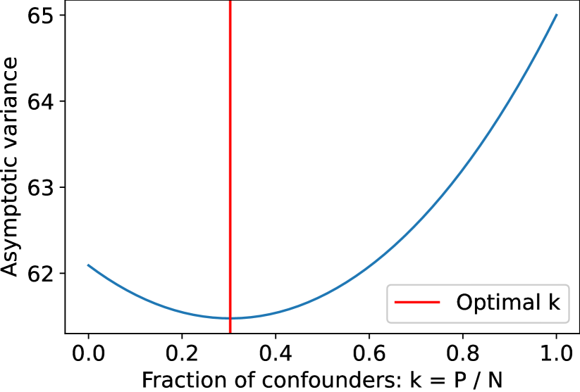
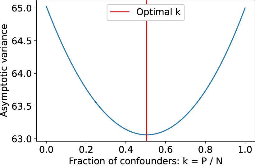
Cramer-Rao Lower Bound   To compute the variance of the estimate of $e=ac$, we compute the Cramer-Rao variance lower bound. We first compute the Fisher information matrix $\mathbf{I}$ as $\mathbf{I}=-\mathbb{E}\left[\nabla^{2}_{\theta}\mathcal{LL}\right]$, where $\theta$ represents the eight model parameters. Let $\widehat{e}$ be the MLE. Since regularity holds for our model (due to linearity and Gaussianity), the MLE is asymptotically normal. Using the Cramer-Rao theorem, for constant $k$, as $N\to\infty$, we have $\sqrt{N}(\widehat{e}-e)\overset{d}{\to}\mathcal{N}(0,V_{e})$, where $V_{e}$ is a function of $\mathbf{I}^{-1}$. The closed form expression for $V_{e}$ is given in Appendix F.1.

For any fixed $k\in(0,1)$, $(V_{e}-\text{AVar}(\sqrt{P}\widehat{ac})_{\text{backdoor}})<0$ and $(V_{e}-\text{AVar}(\sqrt{Q}\widehat{a}_{f}\widehat{c}))<0$, where AVar is asymptotic variance. This shows that the combined estimator always has lower asymptotic variance than that of the backdoor and frontdoor estimators on the individual datasets. Moreover, we also find cases where the combined estimator outperforms both the backdoor and frontdoor estimators even when the total number of samples are the same. That is, there exist model parameters such that $(V_{e}-\text{AVar}(\sqrt{N}\widehat{ac})_{\text{backdoor}})<0$ and $(V_{e}-\text{AVar}(\sqrt{N}\widehat{a}_{f}\widehat{c}))<0$ for some $k\in(0,1)$. This means that is these cases, it is better to collect a mix of confounders and mediators rather than only collecting mediators or confounders. Despite having access to the same number of samples, a mix of confounders and mediators can lead to lower variance. This happens when the variances of the backdoor and frontdoor estimators are close to each other. In Figure 2, we present two examples of causal graphs where having a mix of confounders and mediators leads to the lowest asymptotic variance (see Appendix F.2 for parameter values).

The Maximum Likelihood Estimator   Computing an analytical solution for the model parameters that maximizes the log-likelihood turns out to be intractable. As a result, we update our estimated parameters to maximize the likelihood numerically. The likelihood in Eq. 6 is non-convex. So we intialize the parameters using the two datasets (see Appendix F.3 for details) and run the Broyden–Fletcher–Goldfarb–Shanno (BFGS) algorithm [Fletcher, 2013] to maximize the likelihood. In our experiments, the non-convexity of the likelihood never proved a practical problem. When we find the global minimum, this estimator is optimal and dominates both the backdoor and frontdoor estimators.

7 Experiments

Synthetic Data   To show that the empirical variance of the various estimators is close to the theoretical variance (Table 1), we randomly initialize parameters and for each instance, we compute the Mean and Standard Deviation of Absolute Percentage Error of theoretical variance as a predictor of empirical variance (see Appendix G). Next, we compare the estimators under different settings of the model parameters. Unless stated otherwise, the model parameter values we use for experiments are $a=10,b=4,c=5,d=5,\sigma^{2}_{u_{w}}=1,\sigma^{2}_{u_{x}}=1,\sigma^{2}_{u_{m}}=1,\sigma^{2}_{u_{y}}=1$.

(a) Backdoor better

(b) Frontdoor better

Figure 3: Comparison of MSE when confounders and mediators are observed simultaneously. Either of the backdoor or frontdoor estimators can dominate. The combined estimator is better than both.

(a)

(b)

Figure 4: Comparison of MSE when confounders and mediators are observed in separate datasets. The combined estimator dominates in both cases.

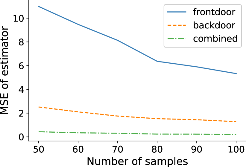
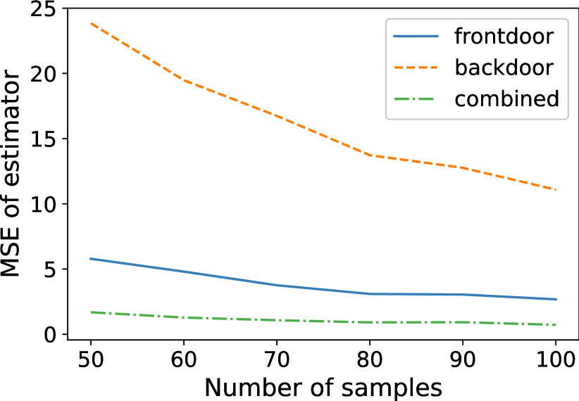
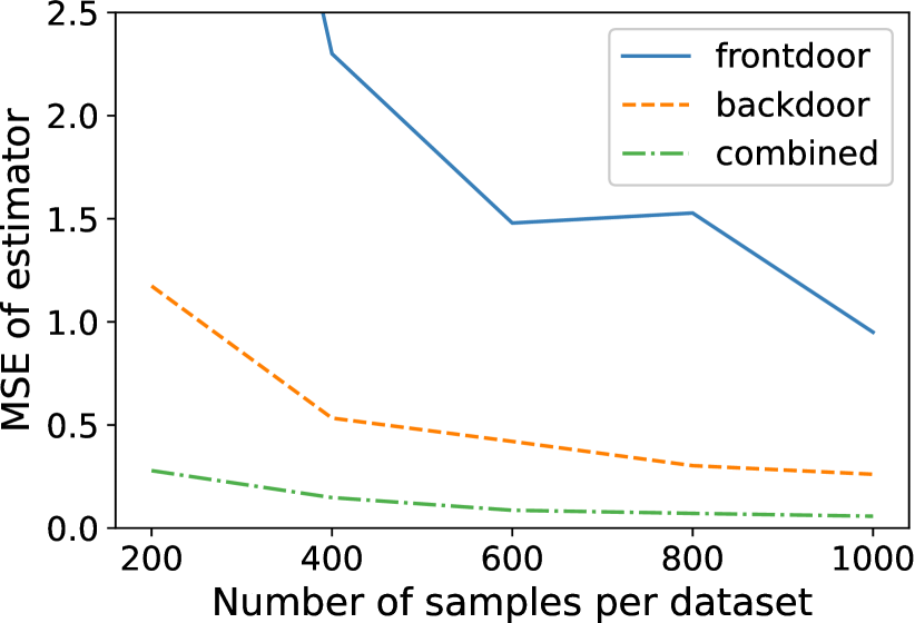
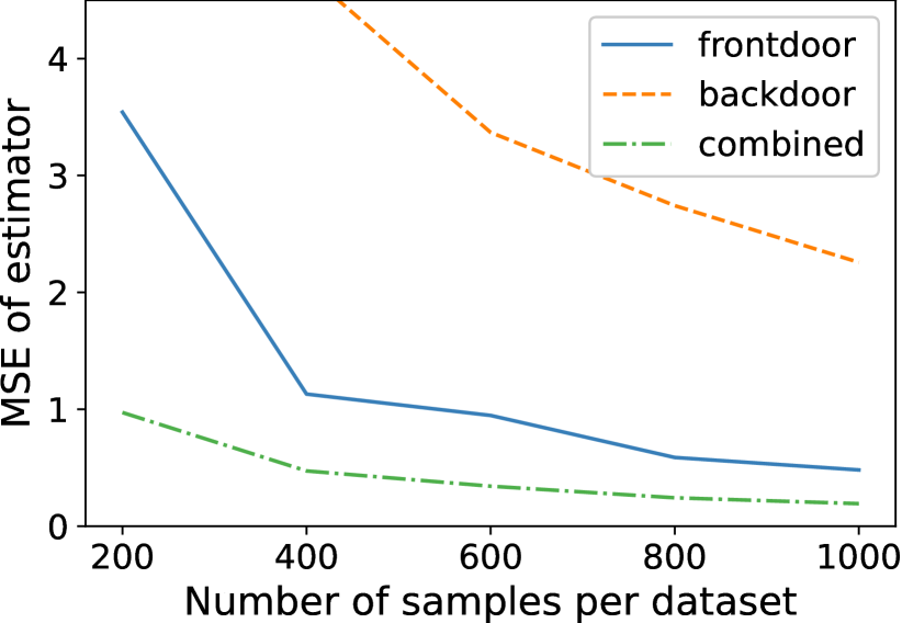
The quantity of interest is the causal effect $ac=50$. For Figure 3(a), we set $\{\sigma^{2}_{u_{x}}=0.05,\sigma^{2}_{u_{m}}=0.05\}$, which makes the backdoor estimator better as predicted by Eq. 10. For Figure 3(b), we set $\{\sigma^{2}_{u_{w}}=2,\sigma^{2}_{u_{x}}=0.01,\sigma^{2}_{u_{m}}=0.1\}$ which makes the frontdoor estimator better as predicted by Eq. 10. The plots in Figure 3(a) and 3(b) corroborate these predictions at different sample sizes. Furthermore, the optimal combined estimator always outperforms both the backdoor and frontdoor estimators.

Next, we evaluate the procedure for combining datasets described in Section 6, generating two datasets with equal numbers of samples. In the first, only $\{X,Y,W\}$ are observed. In the second, only $\{X,Y,M\}$ are observed. We set $\{\sigma^{2}_{u_{x}}=0.05,\sigma^{2}_{u_{m}}=0.05\}$, which makes the backdoor estimator better (Figure 4(a)), and then set $\{\sigma^{2}_{u_{w}}=2,\sigma^{2}_{u_{x}}=0.01,\sigma^{2}_{u_{m}}=0.1\}$, which makes the frondoor estimator better (Figure 4(b)). The plots show that the combined estimator has lower MSE than either for various sample sizes (Figure 4), supporting our theoretical claims.

IHDP Dataset   Hill [2011] constructed a dataset from the Infant Health and Development Program (IHDP). This semi-synthetic dataset has been used for benchmarking in causal inference [Shi et al., 2019, Shalit et al., 2017]. The dataset is is based on a randomized experiment to measure the effect of home visits from a specialist on future cognitive test scores of children. The treatment is binary and the covariates contain both continuous and categorical variables representing measurements on the child and their mother. We use samples from the NPCI package [Dorie, 2016]. We converted the randomized data into an observational study by removing a biased subset of the treated group. This set contains $747$ samples with $25$ covariates.

We use the covariates and the treatment assignment from the real study. We use a procedure similar to Hill [2011] to simulate the mediator and the outcome. The mediator $M$ takes the form $M\sim\mathcal{N}(cX,\sigma^{2}_{u_{m}})$, where $X$ is the treatment. The response $Y$ takes the form $Y\sim\mathcal{N}(aM+w^{\top}\mathbf{b},1)$ where $w$ is the vector of standardized (zero mean and unit variance) covariates and values in the vector $\mathbf{b}$ are randomly sampled (0, 1, 2, 3, 4) with probabilities (0.5, 0.2, 0.15, 0.1, 0.05). The ground truth causal effect is $c\times a$.

We evaluate our estimators and the four IF estimators: IF-Fulcher (IF-Fulc), IF-Restricted (IF-Restr), IF-Frontdoor (IF-FD), and IF-Rotnitzky (IF-Rotz) (Section 5.2). We test the estimators on two settings of the model parameters (Table 2, the Complete dataset setting). The MSE values are computed across 1000 instantiations of the dataset created by simulating the mediators and outcomes. We first evaluate the estimators on the complete dataset of 747 samples. We see that for Setting $1$ (S1): $a=10,c=5,\sigma_{u_{m}}=1$, the backdoor estimator dominates the frontdoor estimator whereas for Setting $2$ (S2): $a=10,c=1,\sigma_{u_{m}}=2$, the frontdoor estimator is better. In both cases, the combined estimator (Section 5) outperforms both estimators. Furthermore, we see that IF-Restricted outperforms IF-Frontdoor, showing the value of leveraging the covariates. Moreover, IF-Restricted also outperforms IF-Fulcher, suggesting that incorporating the additional model restrictions improves performance. Next, we randomly split the data into two sets, one with the confounder observed and the other with the mediator observed, finding that the estimator that combines the datasets (Section 6) outperforms the frontdoor and backdoor estimator (Table 2, the Partial dataset setting). We compute the MSE over 1000 realizations of the dataset.

Table 1: Mean Absolute Percentage Error of the theoretical variance as a predictor of the empirical variance. The values are reported as mean $\pm$ std. The % error is small even for small sample sizes.

Estimator	$n=50$	$n=100$	$n=200$
Backdoor	$0.36\pm.3$	$0.32\pm.2$	$0.34\pm.1$
Frontdoor	$0.33\pm.2$	$0.30\pm.2$	$0.23\pm.1$
Combined	$1.20\pm 1.1$	$0.97\pm.6$	$0.58\pm.2$

Table 2: Results on the IHDP and JTPA datasets. The complete (C) data setting is when $\{W,X,M,Y\}$ are observed and partial (P) is with $\{X,M,Y\}$ and $\{W,X,Y\}$ observed in two separate datasets.

		IHDP MSE		JTPA
Estimator	Data	S1	S2	Var	MSE
Backdoor	C	2.14	1.07	NA	NA
Frontdoor	C	1.97	2.81	40.9k	75.3k
Combined	C	1.78	0.93	33.1k	70.1k
IF-FD	C	4.24	2.07	46.6k	77.9k
IF-Restr	C	3.49	1.48	40.4k	42.1k
IF-Fulc	C	3.82	1.87	45.1k	46.2k
IF-Rotz	C	3.58	2.01	NA	NA
Backdoor	P	5.44	2.43	NA	NA
Frontdoor	P	3.92	4.94	74.8k	115.1k
Combined	P	2.97	1.62	79.5k	123.1k

National JTPA Study   The National Job Training Partnership Act (JTPA) Study evaluates the effect of a job training program on future earnings. We use the dataset from Glynn and Kashin [2019]. The binary treatment $X$ represents if a participant signed up for the program. The outcome $Y$ represents future earnings. The collected covariates (like race, study location, age) are the confounders $W$. The covariates contain both categorical and continuous variables. There was non-compliance among the treated units. The binary mediator $M$ represents compliance, that is, whether the participant make use of JTPA services after signing up. The study contained a randomized component which allowed us to compute the ground truth treatment effect, which was $862.74$. Glynn and Kashin [2018] showed that the backdoor estimator has high bias, suggesting that there was unmeasured confounding, so we omit the backdoor estimator in our results. They also justify the assumptions required for the frontdoor estimator and show that it works well for this study.

A comparison of the frontdoor estimator, the combined estimator (Section 5), IF-Restricted, IF-Frontdoor and IF-Fulcher (Section 5.2) is shown in Table 2 (the “C” data setting). For IF-Restricted, we only use the $f(M|X,W)=f(M|X)$ restriction and do not use the $\mathbb{E}[Y|M,W,X]=\mathbb{E}[Y|M,W]$ restriction since it is not valid. We compute the variance and MSE using 1000 bootstrap iterations. The combined estimator has lower variance and MSE than the frontdoor estimator. IF-Restricted outperforms IF-Frontdoor, reinforcing the utility of combined estimators. Furthermore, IF-Restricted outperforms IF-Fulcher, showing that using model restrictions is valuable. Next, we evaluate our procedure for the partially-observed setting (Section 6). We compute variance and MSE across $1000$ bootstrap iterations. At each iteration, we randomly split our dataset into two datasets of equal size, one with revealed confounders, one with revealed mediators. The combined estimator does not outperform the frontdoor estimator (Table 2, the “P” data setting). This is expected since the backdoor adjustment works poorly and the revealed-confounder data is unlikely to help. Despite this, the combined estimator does not suffer too badly and has low bias despite the required assumptions for one of the identification strategies not holding.

8 Discussion

In this paper, we studied over-identified graphs with confounders and mediators, showing that the two identification strategies can lead to estimators with arbitrarily different variances. We show that having access to both confounders and mediators (either simultaneously or in separate datasets) can give (unbounded) performance gains. We also show that our results qualitatively apply to general non-linear settings.

Future Work

We see several promising lines for future work, including (i) extensions to more general graphs; (ii) online data collection subject to some cost structure over the observations; and (iii) leveraging overidentification to mitigate errors due to measurement and confounding. Our experiments show the applicability of our methods in the frontdoor-backdoor graph, with combined estimators yielding gains in both linear and non-linear settings. We expect these insights to extend to other over-identified settings (e.g. graphs with multiple instrumental variables, multiple confounders, etc.) and we hope next to extend the results to more general over-identified causal graphs. Additionally, we plan to analyze the online data collection setting. Here, subject to budget constraints, a practitioner must choose which variables to observe at each time step. This direction seems especially important in medical applications (where each test may be costly) and survey studies (with a cap on the number of questions). Our current results suggest that the optimal strategy must depend on the model parameters. At each step, the revealed data will improve our estimates of the model parameters, in turn impacting what we collect in the future.

One potential limitation of the method is that situations where there exist multiple valid identification formulas may be uncommon in practice, when finding a single source of identification can already be difficult. However, we believe that in reality, many identification approaches are often available, but members of the community find flaws in each of the proposed estimators. In these cases, with multiple imperfect estimators of the same causal effect, we believe that overidentification might be leveraged to create robust combined estimators.

Appendix A Brief review of OLS regression

Since we use OLS regression for our results, we briefly review OLS estimators. We consider the following setup:

$$\mathbf{y} =\mathbf{X}\mathbf{\beta}+\mathbf{e},$$

where $\mathbf{y}$ and $\mathbf{e}$ are $n\times 1$ vectors, $\mathbf{X}$ is an $n\times d$ matrix of observations, and $\mathbf{\beta}$ is the $d\times 1$ coefficient vector that we want to estimate. If $\mathbf{e}\perp\!\!\!\!\perp\mathbf{X}$ and $\mathbf{e}\sim\mathcal{N}(0,\sigma^{2}_{e}\mathbf{I_{n}})$, where $\mathbf{I_{n}}$ is the $n\times n$ identity matrix, then the OLS estimate of $\mathbf{\beta}$ is

$$\widehat{\mathbf{\beta}} =(\mathbf{X}^{\top}\mathbf{X})^{-1}\mathbf{X}^{\top}\mathbf{y}$$

$$=\mathbf{\beta}+(\mathbf{X}^{\top}\mathbf{X})^{-1}\mathbf{X}^{\top}\mathbf{e},$$

with $\mathbb{E}[\widehat{\mathbf{\beta}}]=\mathbf{\beta}$ and $\text{Var}(\widehat{\mathbf{\beta}})=\sigma^{2}_{e}\mathbb{E}[(\mathbf{X}^{\top}\mathbf{X})^{-1}]$. If each row $X_{i}$ of $\mathbf{X}$ is sampled from $X_{i}\overset{i.i.d.}{\sim}\mathcal{N}(0,\Sigma)$, then the distribution of $(\mathbf{X}^{\top}\mathbf{X})^{-1}$ is an Inverse-Wishart distribution. Then the variance of $\widehat{\mathbf{\beta}}$ is

$$\text{Var}(\widehat{\mathbf{\beta}})=\frac{\sigma^{2}_{e}\Sigma^{-1}}{n-d-1}.$$ (17)

Appendix B Covariance of $\widehat{a}$ and $\widehat{c}$

B.1 Frontdoor estimator

We prove that $\text{Cov}(\widehat{a}_{f},\widehat{c})=0$ for the frontdoor estimator. The expressions for $\widehat{a}_{f}$ and $\widehat{c}$ are

$$\widehat{c} \begin{aligned} &=\frac{\sum x_{i}m_{i}}{\sum x^{2}_{i}}\\ &=c+\frac{\sum x_{i}u^{m}_{i}}{\sum x^{2}_{i}}\end{aligned}$$ (18)

$$\widehat{a}_{f} \begin{aligned} &=\frac{\sum x^{2}_{i}\sum m_{i}y_{i}-\sum x_{i}m_{i}\sum x_{i}y_{i}}{\sum x^{2}_{i}\sum m^{2}_{i}-(\sum x_{i}m_{i})^{2}}\\ &=a+\frac{\sum x^{2}_{i}\sum m_{i}e_{i}-\sum x_{i}m_{i}\sum x_{i}e_{i}}{\sum x^{2}_{i}\sum m^{2}_{i}-(\sum x_{i}m_{i})^{2}},\end{aligned}$$ (19)

where $e_{i}=-\frac{b}{d}u^{x}_{i}+u^{y}_{i}$. Using the fact the $(u^{x},x)$ is bivariate normally distributed, we get

$$\mathbb{E}[e|x] =\frac{b\sigma^{2}_{u_{x}}}{d(d^{2}\sigma^{2}_{u_{w}}+\sigma^{2}_{u_{x}})}x$$

$$=Fx,$$ (20)

where $F=\frac{b\sigma^{2}_{u_{x}}}{d(d^{2}\sigma^{2}_{u_{w}}+\sigma^{2}_{u_{x}})}$. The covariance then is

$$\text{Cov}(\widehat{a}_{f},\widehat{c}) =\mathbb{E}[(\widehat{a}_{f}-a)(\widehat{c}-c)]$$

$$=\mathbb{E}[\mathbb{E}[(\widehat{a}_{f}-a)(\widehat{c}-c)|x,m]]$$

$$=\mathbb{E}\bigg{[}\mathbb{E}\bigg{[}\left(\frac{\sum x^{2}_{i}\sum m_{i}e_{i}-\sum x_{i}m_{i}\sum m_{i}e_{i}}{\sum x^{2}_{i}\sum m^{2}_{i}-(\sum x_{i}m_{i})^{2}}\right)\left(\frac{\sum x_{i}u^{m}_{i}}{\sum x^{2}_{i}}\right)\bigg{|}x,m\bigg{]}\bigg{]}$$

$$=\mathbb{E}\bigg{[}\left(\frac{\sum x^{2}_{i}\sum m_{i}\mathbb{E}[e_{i}|x]-\sum m_{i}x_{i}\sum x_{i}\mathbb{E}[e_{i}|x]}{\sum x^{2}_{i}\sum m^{2}_{i}-(\sum x_{i}m_{i})^{2}}\right)\left(\frac{\sum u^{m}_{i}x_{i}}{\sum x^{2}_{i}}\right)\bigg{]}$$ (21)

$$=\mathbb{E}\bigg{[}F\left(\frac{\sum x^{2}_{i}\sum m_{i}x_{i}-\sum m_{i}x_{i}\sum x^{2}_{i}}{\sum x^{2}_{i}\sum m^{2}_{i}-(\sum x_{i}m_{i})^{2}}\right)\left(\frac{\sum u^{m}_{i}x_{i}}{\sum x^{2}_{i}}\right)\bigg{]}$$

$$=0,$$

where in Eq. 21 we used the expression from Eq. 20. Also, in Eq. 21, we took $u^{m}_{i}$ out of the conditional expectation because $u^{m}_{i}$ is given $x_{i}$ and $m_{i}$ (because $u^{m}_{i}=m_{i}-cx_{i}$).

B.2 Combined estimator

We prove that $\text{Cov}(\widehat{a}_{c},\widehat{c})=0$ for the combined estimator from Section 5. The expressions for $\widehat{a}_{c}$ and $\widehat{c}$ are

$$\widehat{c} \begin{aligned} &=\frac{\sum x_{i}m_{i}}{\sum x^{2}_{i}}\\ &=c+\frac{\sum x_{i}u^{m}_{i}}{\sum x^{2}_{i}}\end{aligned}$$ (22)

$$\widehat{a}_{c} \begin{aligned} &=\frac{\sum w^{2}_{i}\sum m_{i}y_{i}-\sum w_{i}m_{i}\sum w_{i}y_{i}}{\sum w^{2}_{i}\sum m^{2}_{i}-(\sum w_{i}m_{i})^{2}}\\ &=a+\frac{\sum w^{2}_{i}\sum m_{i}u^{y}_{i}-\sum w_{i}m_{i}\sum w_{i}u^{y}_{i}}{\sum w^{2}_{i}\sum m^{2}_{i}-(\sum w_{i}m_{i})^{2}}.\end{aligned}$$ (23)

The covariance is

$$\text{Cov}(\widehat{a}_{c},\widehat{c}) =\mathbb{E}[(\widehat{a}_{c}-a)(\widehat{c}-c)]$$

$$=\mathbb{E}[\mathbb{E}[(\widehat{a}_{c}-a)(\widehat{c}-c)|x,m,w]]$$

$$=\mathbb{E}\bigg{[}\bigg{(}\frac{\sum w^{2}_{i}\sum m_{i}\mathbb{E}[u^{y}_{i}]-\sum m_{i}w_{i}\sum w_{i}\mathbb{E}[u^{y}_{i}]}{\sum w^{2}_{i}\sum m^{2}_{i}-(\sum w_{i}m_{i})^{2}}\bigg{)}\bigg{(}\frac{\sum u^{m}_{i}x_{i}}{\sum x^{2}_{i}}\bigg{)}\bigg{]}$$ (24)

$$=0,$$

where in 24 we used the fact that $\mathbb{E}[u^{y}_{i}]=0$.

Appendix C Unbiasedness of the estimators

C.1 Backdoor estimator

Recall that for the backdoor estimator, we take the coefficient of $X$ in an OLS regression of $Y$ on $\{X,W\}$. The outcome $y_{i}$ can be written as

$$y_{i}=acx_{i}+bw_{i}+au^{m}_{i}+u^{y}_{i}.$$

The error term $au^{m}_{i}+u^{y}_{i}$ is independent of $(x_{i},w_{i})$. In this case, the OLS estimator is unbiased. Therefore, $\mathbb{E}[\widehat{ac}_{\text{backdoor}}]=ac$.

C.2 Frontdoor estimator

For the frontdoor estimator, we first compute $\widehat{c}$ by taking the coefficient of $X$ in an OLS regression of $M$ on $X$. The mediator $m_{i}$ can be written as

$$m_{i}=cx_{i}+u^{m}_{i}.$$

The error term $u^{m}_{i}$ is independent of $x_{i}$. In this case, the OLS estimator is unbiased and hence, $\mathbb{E}[\widehat{c}]=c$.

We then compute $\widehat{a}_{f}$ by taking the coefficient of $M$ in an OLS regression of $Y$ on $\{M,X\}$. The outcome $y_{i}$ can be written as

$$y_{i} =am_{i}+\frac{b}{d}x_{i}-\frac{b}{d}u^{x}_{i}+u^{y}.$$

In this case, the error term $-\frac{b}{d}u^{x}_{i}+u^{y}$ is correlated with $x_{i}$. The expression for $\widehat{a}$ is given in Eq. 19. The expectation $\mathbb{E}[\widehat{a}_{f}]$ is

$$\mathbb{E}[\widehat{a}_{f}] =a+\mathbb{E}\left[\frac{\sum x^{2}_{i}\sum m_{i}e_{i}-\sum x_{i}m_{i}\sum x_{i}e_{i}}{\sum x^{2}_{i}\sum m^{2}_{i}-(\sum x_{i}m_{i})^{2}}\right]$$

$$=a+\mathbb{E}\left[\mathbb{E}\left[\frac{\sum x^{2}_{i}\sum m_{i}e_{i}-\sum x_{i}m_{i}\sum x_{i}e_{i}}{\sum x^{2}_{i}\sum m^{2}_{i}-(\sum x_{i}m_{i})^{2}}\bigg{|}x,m\right]\right]$$

$$=a+\mathbb{E}\left[\frac{\sum x^{2}_{i}\sum m_{i}\mathbb{E}[e_{i}|x]-\sum x_{i}m_{i}\sum x_{i}\mathbb{E}[e_{i}|x]}{\sum x^{2}_{i}\sum m^{2}_{i}-(\sum x_{i}m_{i})^{2}}\right]$$ (25)

$$=a+\mathbb{E}\left[\frac{\sum x^{2}_{i}\sum m_{i}(Fx_{i})-\sum x_{i}m_{i}\sum x_{i}(Fx_{i})}{\sum x^{2}_{i}\sum m^{2}_{i}-(\sum x_{i}m_{i})^{2}}\right]$$

$$=a,$$

where, in Eq. 25, the expression for $E[e_{i}|x]$ is taken from Eq. 20. Using the fact that $\text{Cov}(\widehat{a}_{f},\widehat{c})=0$ (see proof in Appendix B.1), we can see that the frontdoor estimator is unbiased as

$$\mathbb{E}[\widehat{a}_{f}\widehat{c}] =\mathbb{E}[\widehat{a}_{f}]\mathbb{E}[\widehat{c}]+\text{Cov}(\widehat{a}_{f},\widehat{c})$$

$$=ac.$$

C.3 Combined estimator

In the combined estimator, the expression for $\widehat{c}$ is the same as for the frontdoor estimator. Therefore, as shown in Appendix C.2, $\mathbb{E}[\widehat{c}]=c$. We compute $\widehat{a}$ by taking the coefficient of $M$ in an OLS regression of $Y$ on $\{M,W\}$. The outcome $y_{i}$ can be written as

$$y_{i}=am_{i}+bw_{i}+u^{y}_{i}.$$

The error term $u^{y}_{i}$ is independent of $(m_{i},w_{i})$. In this case, the OLS estimator is unbiased. Therefore, $\mathbb{E}[\widehat{a}_{c}]=a$. Using the fact that $\text{Cov}(\widehat{a}_{c},\widehat{c})=0$ (see proof Appendix B.2), we can see that the combined estimator is unbiased as

$$\mathbb{E}[\widehat{a}_{c}\widehat{c}] =\mathbb{E}[\widehat{a}_{c}]\mathbb{E}[\widehat{c}]+\text{Cov}(\widehat{a}_{c},\widehat{c})$$

$$=ac.$$

Appendix D Variance results for the frontdoor, backdoor, and combined estimators

D.1 Backdoor estimator

The outcome $y_{i}$ can be written as

$$y_{i}=acx_{i}+bw_{i}+au^{m}_{i}+u^{y}_{i}.$$

We estimate the causal effect $ac$ by taking the coefficient on $X$ in an OLS regression of $Y$ on $\{X,W\}$. Let $\Sigma=\text{Cov}([X,W])$. Using Eq. 17, the finite sample variance of the backdoor estimator is

$$\text{Var}(\widehat{ac})_{\text{backdoor}} =\frac{\text{Var}(au^{m}+u^{y})\left(\Sigma^{-1}\right)_{1,1}}{n-3}$$

$$=\frac{a^{2}\sigma^{2}_{u_{m}}+\sigma^{2}_{u_{y}}}{(n-3)\sigma^{2}_{u_{x}}}.$$

OLS estimators are asymptotically normally for arbitrary error distributions (and hence, Gaussianity is not needed). Therefore, the asymptotic variance of the backdoor estimator is

$$\lim_{n\to\infty}\text{Var}(\sqrt{n}(\widehat{ac}-ac))_{\text{backdoor}} =\text{Var}(au^{m}+u^{y})\left(\Sigma^{-1}\right)_{1,1}=\frac{a^{2}\sigma^{2}_{u_{m}}+\sigma^{2}_{u_{y}}}{\sigma^{2}_{u_{x}}}.$$

D.2 Frontdoor estimator

D.2.1 Variance of $\widehat{c}$

The regression of $M$ on $X$ can be written as $m_{i}=cx_{i}+u^{m}_{i}$. Let $\Sigma_{c}=\text{Var}(X)$. Using Eq. 17, $\text{Var}(\widehat{c})$ is

$$\text{Var}(\widehat{c}) =\frac{\text{Var}(u^{m})(\Sigma^{-1}_{c})}{n-2}=\frac{\sigma^{2}_{u_{m}}}{(n-2)(d^{2}\sigma^{2}_{u_{w}}+\sigma^{2}_{u_{x}})}.$$

D.2.2 Variance of $\widehat{a}_{f}$

The regression of $Y$ on $\{M,X\}$ can be written as $y_{i}=am_{i}+\frac{b}{d}x_{i}+e_{i}$, where $e_{i}=-\frac{b}{d}u^{x}_{i}+u^{y}_{i}$. In this case, the error $e_{i}$ is not independent of the regressor $x_{i}$. Using the fact that $(u^{x},x)$ has a bivariate normal distribution, $\text{Var}(e|x)$ is

$$\text{Var}(e|x) =\frac{b^{2}\sigma^{2}_{u_{w}}\sigma^{2}_{u_{x}}+\sigma^{2}_{u_{y}}(d^{2}\sigma^{2}_{u_{w}}+\sigma^{2}_{u_{x}})}{(d^{2}\sigma^{2}_{u_{w}}+\sigma^{2}_{u_{x}})}$$ (26)

$$:=V_{e}.$$

Note that $V_{e}$ is a constant and does not depend on $x$. From Eqs. 18 and 19, we know that

$$\widehat{c} =c+\frac{\sum x_{i}u^{m}_{i}}{\sum x^{2}_{i}}$$

$$\widehat{a}_{f} =a+\frac{\sum x^{2}_{i}\sum m_{i}e_{i}-\sum x_{i}m_{i}\sum x_{i}e_{i}}{\sum x^{2}_{i}\sum m^{2}_{i}-(\sum x_{i}m_{i})^{2}}.$$

where $e_{i}=-\frac{b}{d}u^{x}_{i}+u^{y}_{i}$. Let

$$A =\frac{\sum x^{2}_{i}\sum m_{i}e_{i}-\sum x_{i}m_{i}\sum x_{i}e_{i}}{\sum x^{2}_{i}\sum m^{2}_{i}-(\sum x_{i}m_{i})^{2}}$$

$$C =\frac{\sum x_{i}u^{m}_{i}}{\sum x^{2}_{i}}.$$

First, we derive the expression for $\text{Var}(\widehat{a}_{f})$ as follows,

$$\text{Var}(\widehat{a}_{f}) =\text{Var}(a+A)$$

$$=\text{Var}(A)$$

$$=\text{Var}(\mathbb{E}[A|x,m])+\mathbb{E}[\text{Var}(A|x,m)]$$

$$=\text{Var}\left(\mathbb{E}\left[\frac{\sum x^{2}_{i}\sum m_{i}e_{i}-\sum x_{i}m_{i}\sum x_{i}e_{i}}{\sum x^{2}_{i}\sum m^{2}_{i}-(\sum x_{i}m_{i})^{2}}\bigg{|}x,m\right]\right)+\mathbb{E}[\text{Var}(A|x,m)]$$

$$=\text{Var}\left(\mathbb{E}\left[\frac{\sum x^{2}_{i}\sum m_{i}\mathbb{E}[e_{i}|x]-\sum x_{i}m_{i}\sum x_{i}\mathbb{E}[e_{i}|x]}{\sum x^{2}_{i}\sum m^{2}_{i}-(\sum x_{i}m_{i})^{2}}\right]\right)+\mathbb{E}[\text{Var}(A|x,m)]$$ (27)

$$=\text{Var}\left(\mathbb{E}\left[\frac{\sum x^{2}_{i}\sum m_{i}(Fx_{i})-\sum x_{i}m_{i}\sum x_{i}(Fx_{i})}{\sum x^{2}_{i}\sum m^{2}_{i}-(\sum x_{i}m_{i})^{2}}\right]\right)+\mathbb{E}[\text{Var}(A|x,m)]$$

$$=\mathbb{E}[\text{Var}(A|x,m)]$$

$$=\mathbb{E}\left[\text{Var}\left(\frac{\sum x^{2}_{i}\sum m_{i}e_{i}-\sum x_{i}m_{i}\sum x_{i}e_{i}}{\sum x^{2}_{i}\sum m^{2}_{i}-(\sum x_{i}m_{i})^{2}}\bigg{|}x,m\right)\right]$$

$$=\mathbb{E}\left[\frac{1}{\left(\sum x^{2}_{i}\sum m^{2}_{i}-(\sum x_{i}m_{i})^{2}\right)^{2}}\text{Var}\left(\sum x^{2}_{i}\sum m_{i}e_{i}-\sum x_{i}m_{i}\sum x_{i}e_{i}\bigg{|}x,m\right)\right]$$

$$=\mathbb{E}\left[\frac{1}{\left(\sum x^{2}_{i}\sum m^{2}_{i}-(\sum x_{i}m_{i})^{2}\right)^{2}}\text{Var}(e_{i}|x_{i})\sum x^{2}_{i}\left(\sum x^{2}_{i}\sum m^{2}_{i}-(\sum x_{i}m_{i})^{2}\right)\right]$$

$$=V_{e}\mathbb{E}\left[\frac{\sum x^{2}_{i}}{\sum x^{2}_{i}\sum m^{2}_{i}-(\sum x_{i}m_{i})^{2}}\right]$$

$$=V_{e}\mathbb{E}\left[D\right],$$ (28)

where, in Eq. 27, we used the result from Eq. 20, and $D=\frac{\sum x^{2}_{i}}{\sum x^{2}_{i}\sum m^{2}_{i}-(\sum x_{i}m_{i})^{2}}$. Using the fact that $D$ has the distribution of a marginal from an inverse Wishart-distributed matrix, that is, if the matrix $M\sim\mathcal{IW}(\text{Cov}([M,X])^{-1},n)$, then $D=M_{1,1}$, in Eq. 28, we get

$$\text{Var}(\widehat{a}_{f}) =V_{e}\mathbb{E}\left[D\right]$$

$$=V_{e}\frac{\text{Cov}([M,X])^{-1}_{1,1}}{n-2-1}$$

$$=\frac{b^{2}\sigma^{2}_{u_{w}}\sigma^{2}_{u_{x}}+\sigma^{2}_{u_{y}}(d^{2}\sigma^{2}_{u_{w}}+\sigma^{2}_{u_{x}})}{(n-3)(d^{2}\sigma^{2}_{u_{w}}+\sigma^{2}_{u_{x}})\sigma^{2}_{u_{m}}},$$

where the expression for $V_{e}$ is taken from Eq. 26.

D.2.3 Covariance of $\widehat{a}_{f}^{2}$ and $\widehat{c}^{2}$

We prove that $\text{Cov}(\widehat{a}_{f}^{2},\widehat{c}^{2})=\text{Var}(\widehat{a}_{f})\text{Var}(\widehat{c})$. This covariance can be written as

$$\text{Cov}(\widehat{a}_{f}^{2},\widehat{c}^{2}) =\mathbb{E}[(\widehat{a}_{f}^{2}-\mathbb{E}[\widehat{a}_{f}^{2}])(\widehat{c}^{2}-\mathbb{E}[\widehat{c^{2}}])]$$

$$=\mathbb{E}[(\widehat{a}_{f}^{2}-\text{Var}(\widehat{a}_{f})-\mathbb{E}^{2}[\widehat{a}_{f}])(\widehat{c}^{2}-\text{Var}(\widehat{c})-\mathbb{E}^{2}[\widehat{c}])]$$

$$=\mathbb{E}[\widehat{a}_{f}^{2}\widehat{c}^{2}]-\text{Var}(\widehat{a}_{f})\text{Var}(\widehat{c})-a^{2}\text{Var}(\widehat{c})-c^{2}\text{Var}(\widehat{a}_{f})-a^{2}c^{2}.$$ (29)

We can write $\mathbb{E}[\widehat{a}_{f}^{2}\widehat{c}^{2}]$ as

$$\mathbb{E}[\widehat{a}_{f}^{2}\widehat{c}^{2}] =\mathbb{E}[(a+A)^{2}(c+C)^{2}]$$

$$=\mathbb{E}[a^{2}c^{2}+c^{2}A^{2}+a^{2}C^{2}+A^{2}C^{2}+2aAC^{2}+2cCA^{2}]$$

$$=a^{2}c^{2}+c^{2}\text{Var}(\widehat{a})+a^{2}\text{Var}(\widehat{c})+\mathbb{E}[A^{2}C^{2}]+\mathbb{E}[2aAC^{2}]+\mathbb{E}[2cCA^{2}].$$ (30)

Substituting the result from Eq. 30 in Eq. 29, we get

$$\text{Cov}(\widehat{a}_{f}^{2},\widehat{c}^{2}) =\mathbb{E}[A^{2}C^{2}]+\mathbb{E}[2aAC^{2}]+\mathbb{E}[2cCA^{2}].$$ (31)

Now we expand each term in Eq. 31 separately. $\mathbb{E}[2aAC^{2}]$ is

$$\mathbb{E}[2aAC^{2}] =2a\mathbb{E}\left[\left(\frac{\sum x_{i}u^{m}_{i}}{\sum x^{2}_{i}}\right)^{2}\left(\frac{\sum x^{2}_{i}\sum m_{i}e_{i}-\sum x_{i}m_{i}\sum x_{i}e_{i}}{\sum x^{2}_{i}\sum m^{2}_{i}-(\sum x_{i}m_{i})^{2}}\right)\right]$$

$$=2a\mathbb{E}\left[\mathbb{E}\left[\left(\frac{\sum x_{i}u^{m}_{i}}{\sum x^{2}_{i}}\right)^{2}\left(\frac{\sum x^{2}_{i}\sum m_{i}e_{i}-\sum x_{i}m_{i}\sum x_{i}e_{i}}{\sum x^{2}_{i}\sum m^{2}_{i}-(\sum x_{i}m_{i})^{2}}\right)\Bigg{|}{x,m}\right]\right]$$

$$=2a\mathbb{E}\left[\left(\frac{\sum x_{i}u^{m}_{i}}{\sum x^{2}_{i}}\right)^{2}\left(\frac{\sum x^{2}_{i}\sum m_{i}\mathbb{E}[e_{i}|x]-\sum x_{i}m_{i}\sum x_{i}\mathbb{E}[e_{i}|x]}{\sum x^{2}_{i}\sum m^{2}_{i}-(\sum x_{i}m_{i})^{2}}\right)\right]$$ (32)

$$=2a\mathbb{E}\left[\left(\frac{\sum x_{i}u^{m}_{i}}{\sum x^{2}_{i}}\right)^{2}\left(\frac{\sum x^{2}_{i}\sum m_{i}(Fx_{i})-\sum x_{i}m_{i}\sum x_{i}(Fx_{i})}{\sum x^{2}_{i}\sum m^{2}_{i}-(\sum x_{i}m_{i})^{2}}\right)\right]$$

$$=0,$$ (33)

where, in Eq. 32, the expression for $\mathbb{E}[e|x]$ is taken from Eq. 20.

Next, we simplify $\mathbb{E}[2cCA^{2}]$ as

$$\mathbb{E}[ 2cCA^{2}]$$

$$=2c\mathbb{E}\left[\left(\frac{\sum x_{i}u^{m}_{i}}{\sum x^{2}_{i}}\right)\left(\frac{\sum x^{2}_{i}\sum m_{i}e_{i}-\sum x_{i}m_{i}\sum x_{i}e_{i}}{\sum x^{2}_{i}\sum m^{2}_{i}-(\sum x_{i}m_{i})^{2}}\right)^{2}\right]$$

$$=2c\mathbb{E}\left[\mathbb{E}\left[\left(\frac{\sum x_{i}u^{m}_{i}}{\sum x^{2}_{i}}\right)\left(\frac{\sum x^{2}_{i}\sum m_{i}e_{i}-\sum x_{i}m_{i}\sum x_{i}e_{i}}{\sum x^{2}_{i}\sum m^{2}_{i}-(\sum x_{i}m_{i})^{2}}\right)^{2}\Bigg{|}x,m\right]\right]$$

$$=2c\mathbb{E}\left[\mathbb{E}\left[\left(\frac{\sum x_{i}u^{m}_{i}}{\sum x^{2}_{i}}\right)\frac{(\sum x^{2}_{i})^{2}(\sum m_{i}e_{i})^{2}+(\sum x_{i}m_{i})^{2}(\sum x_{i}e_{i})^{2}-2\sum x^{2}_{i}\sum m_{i}e_{i}\sum x_{i}m_{i}\sum x_{i}e_{i}}{\left(\sum x^{2}_{i}\sum m^{2}_{i}-(\sum x_{i}m_{i})^{2}\right)^{2}}\Bigg{|}x,m\right]\right]$$

$$=2c\mathbb{E}\left[\left(\frac{\sum x_{i}u^{m}_{i}}{\sum x^{2}_{i}}\right)\left(\frac{\text{Var}(e|x)(\sum x^{2}_{i})}{\sum x^{2}_{i}\sum m^{2}_{i}-(\sum x_{i}m_{i})^{2}}+\frac{F^{2}\left(2(\sum x^{2}_{i})^{2}(\sum x_{i}m_{i})^{2}-2(\sum x^{2}_{i})^{2}(\sum x_{i}m_{i})^{2}\right)}{\left(\sum x^{2}_{i}\sum m^{2}_{i}-(\sum x_{i}m_{i})^{2}\right)^{2}}\right)\right]$$

$$=2c\mathbb{E}\left[\left(\frac{\sum x_{i}u^{m}_{i}}{\sum x^{2}_{i}}\right)\left(\frac{\text{Var}(e|x)(\sum x^{2}_{i})}{\sum x^{2}_{i}\sum m^{2}_{i}-(\sum x_{i}m_{i})^{2}}\right)\right]$$

$$=2cV_{e}\mathbb{E}\left[\left(\frac{\sum x_{i}u^{m}_{i}}{\sum x^{2}_{i}}\right)\left(\frac{\sum x^{2}_{i}}{\sum x^{2}_{i}\sum m^{2}_{i}-(\sum x_{i}m_{i})^{2}}\right)\right]$$

$$=2cV_{e}\mathbb{E}\left[\left(\widehat{c}-c\right)\left(\frac{\sum x^{2}_{i}}{\sum x^{2}_{i}\sum m^{2}_{i}-(\sum x_{i}m_{i})^{2}}\right)\right]$$

$$=2cV_{e}\left(\mathbb{E}\left[\widehat{c}\left(\frac{\sum x^{2}_{i}}{\sum x^{2}_{i}\sum m^{2}_{i}-(\sum x_{i}m_{i})^{2}}\right)\right]-c\mathbb{E}\left[\left(\frac{\sum x^{2}_{i}}{\sum x^{2}_{i}\sum m^{2}_{i}-(\sum x_{i}m_{i})^{2}}\right)\right]\right)$$

$$=2cV_{e}\left(\mathbb{E}\left[\widehat{c}D\right]-c\mathbb{E}\left[D\right]\right),$$ (34)

where $D=\frac{\sum x^{2}_{i}}{\sum x^{2}_{i}\sum m^{2}_{i}-(\sum x_{i}m_{i})^{2}}$. Using the fact that $\widehat{c}$ and $D$ are independent of each other (see proof at the end of this section), we get

$$\mathbb{E}[\widehat{c}D] =\mathbb{E}[\widehat{c}]\mathbb{E}[D]$$

$$=c\mathbb{E}[D].$$ (35)

Substituting the result from Eq. 35 in Eq. 34, we get

$$\mathbb{E}[2cCA^{2}] =2cV_{e}\left(c\mathbb{E}\left[D\right]-c\mathbb{E}\left[D\right]\right)$$

$$=0.$$ (36)

We proceed similarly to Eq. 34 to write $\mathbb{E}[A^{2}C^{2}]$ as

$$\mathbb{E}[A^{2}C^{2}] =V_{e}\mathbb{E}[C^{2}D].$$

Then we further simplify $\mathbb{E}[A^{2}C^{2}]$ as

$$\mathbb{E}[A^{2}C^{2}] =V_{e}\mathbb{E}[C^{2}D]$$

$$=V_{e}\mathbb{E}[(\widehat{c}-c)^{2}D]$$

$$=V_{e}\left(\mathbb{E}\left[\widehat{c}^{2}\right]\mathbb{E}[D]-c^{2}\mathbb{E}[D]\right)$$

$$=V_{e}\left(\text{Var}(\widehat{c})\mathbb{E}[D]+\mathbb{E}^{2}\left[\widehat{c}\right]\mathbb{E}[D]-c^{2}\mathbb{E}[D]\right)$$

$$=V_{e}\text{Var}(\widehat{c})\mathbb{E}[D]$$ (37)

$$=V_{e}\text{Var}(\widehat{c})\frac{\text{Cov}([M,X])^{-1}_{1,1}}{n-2-1}$$

$$=\frac{V_{e}}{(n-3)\sigma^{2}_{u_{m}}}\text{Var}(\widehat{c})$$ (38)

$$=\text{Var}(\widehat{a}_{f})\text{Var}(\widehat{c}),$$ (39)

where, in Eq. 37, we used the fact that if the matrix $M\sim\mathcal{IW}(\text{Cov}([M,X])^{-1},n)$, then $D=M_{1,1}$ (that is, $D$ has the distribution of a marginal from an inverse Wishart-distributed matrix), and in Eq. 38, the expression for $V_{e}$ is taken from Eq. 26.

Substituting the results from Eqs. 33, 36, and 39 in Eq. 31, we get

$$\text{Cov}(\widehat{a}_{f}^{2},\widehat{c}^{2}) =\text{Var}(\widehat{a}_{f})\text{Var}(\widehat{c}).$$ (40)

Proof that $\widehat{c}$ and $D$ are independent.

Let $\Sigma$ be the following sample covariance matrix:

$$\Sigma=\frac{1}{n}\begin{bmatrix}\sum m^{2}_{i}&\sum m_{i}x_{i}\\ \sum m_{i}x_{i}&\sum x^{2}_{i}\end{bmatrix}.$$

The distribution of $\Sigma$ is a Wishart distribution. That is, $\Sigma\sim\mathcal{W}(\text{Cov}([M,X]),n)$. Then $(\Sigma_{1,1}-\Sigma_{1,2}\Sigma_{2,2}^{-1}\Sigma_{2,1})$ and $(\Sigma_{2,1},\Sigma_{2,2})$ are independent [Eaton, 2007, Proposition 8.7]. We can see that

$$\Sigma_{1,1}-\Sigma_{1,2}\Sigma_{2,2}^{-1}\Sigma_{2,1} =\frac{\sum m^{2}_{i}\sum x^{2}_{i}-\left(\sum x_{i}m_{i}\right)^{2}}{\sum x^{2}_{i}}$$

$$=\frac{1}{D}.$$

Therefore, we get

$$\frac{1}{D} \perp\!\!\!\!\perp\left(\sum x^{2}_{i},\sum x_{i}m_{i}\right)$$

$$\therefore\,\,D \perp\!\!\!\!\perp\left(\sum x^{2}_{i},\sum x_{i}m_{i}\right)$$

$$\therefore\,\,D \perp\!\!\!\!\perp\frac{\sum x_{i}m_{i}}{\sum x^{2}_{i}}$$

$$\therefore\,\,D \perp\!\!\!\!\perp\widehat{c}.$$

D.2.4 Finite Sample Variance of $\widehat{a}_{f}\widehat{c}$

The variance of the product of two random variables can be written as

$$\text{Var}(\widehat{a}_{f}\widehat{c}) =\text{Cov}(\widehat{a}_{f}^{2},\widehat{c}^{2})+(\text{Var}(\widehat{a}_{f})+\mathbb{E}^{2}[\widehat{a}_{f}])(\text{Var}(\widehat{c})+\mathbb{E}^{2}[\widehat{c}])-(\text{Cov}(\widehat{a}_{f},\widehat{c})+\mathbb{E}[\widehat{a}_{f}]\mathbb{E}[\widehat{c}])^{2}$$ (41)

$$=\text{Cov}(\widehat{a}_{f}^{2},\widehat{c}^{2})+(\text{Var}(\widehat{a}_{f})+a^{2})(\text{Var}(\widehat{c})+c^{2})-(\text{Cov}(\widehat{a}_{f},\widehat{c})+ac)^{2},$$

where in Eq. 41 we used the facts that $\mathbb{E}[\widehat{a}_{f}]=a$, and $\mathbb{E}[\widehat{c}]=c$ (see Appendix C.2). Using the facts that $\text{Cov}(\widehat{a}_{f}^{2},\widehat{c}^{2})=\text{Var}(\widehat{a}_{f})\text{Var}(\widehat{c})$ (from Eq. 39) and $\text{Cov}(\widehat{a}_{f},\widehat{c})=0$ (from Appendix B.1), we get

$$\text{Var}(\widehat{a}_{f}\widehat{c}) =a^{2}\text{Var}(\widehat{c})+c^{2}\text{Var}(\widehat{a}_{f})+2\text{Var}(\widehat{c})\text{Var}(\widehat{a}_{f}).$$

D.2.5 Asymptotic Variance of $\widehat{a}_{f}\widehat{c}$

Using asymptotic normality of OLS estimators, which does not require Gaussianity, we have

$$\sqrt{n}\left(\begin{bmatrix}\widehat{a}_{f}\\ \widehat{c}\end{bmatrix}-\begin{bmatrix}a\\ c\end{bmatrix}\right) \overset{d}{\to}\mathcal{N}\left(0,\lim_{n\to\infty}\begin{bmatrix}\text{Var}_{\infty}(\widehat{a}_{f})&\text{Cov}(\sqrt{n}\widehat{a}_{f},\widehat{c})\\ \text{Cov}(\sqrt{n}\widehat{a}_{f},\widehat{c})&\text{Var}_{\infty}(\widehat{c})\end{bmatrix}\right)$$

$$\therefore\,\,\sqrt{n}\left(\begin{bmatrix}\widehat{a}_{f}\\ \widehat{c}\end{bmatrix}-\begin{bmatrix}a\\ c\end{bmatrix}\right) \overset{d}{\to}\mathcal{N}\left(0,\begin{bmatrix}\text{Var}_{\infty}(\widehat{a}_{f})&0\\ 0&\text{Var}_{\infty}(\widehat{c})\end{bmatrix}\right),$$

where $\text{Var}_{\infty}(\widehat{a}_{f})$ and $\text{Var}_{\infty}(\widehat{c})$ are the asymptotic variances of $\widehat{a}_{f}$ and $\widehat{c}$, respectively. The expressions for asymptotic variances are

$$\text{Var}_{\infty}(\widehat{a}_{f}) =V_{e}\text{Cov}([M,X])^{-1}_{1,1}=\frac{b^{2}\sigma^{2}_{u_{w}}\sigma^{2}_{u_{x}}+\sigma^{2}_{u_{y}}(d^{2}\sigma^{2}_{u_{w}}+\sigma^{2}_{u_{x}})}{(d^{2}\sigma^{2}_{u_{w}}+\sigma^{2}_{u_{x}})\sigma^{2}_{u_{m}}}$$

$$\text{Var}_{\infty}(\widehat{c}) =\text{Var}(u^{m})(\Sigma^{-1}_{c})=\frac{\sigma^{2}_{u_{m}}}{d^{2}\sigma^{2}_{u_{w}}+\sigma^{2}_{u_{x}}}.$$

In order to compute the asymptotic variance of $\widehat{a}_{f}\widehat{c}$, we use the Delta method:

$$\sqrt{n}(\widehat{a}_{f}\widehat{c}-ac) \overset{d}{\to}\mathcal{N}\left(0,\begin{bmatrix}c&a\end{bmatrix}\begin{bmatrix}\text{Var}_{\infty}(\widehat{a}_{f})&0\\ 0&\text{Var}_{\infty}(\widehat{c})\end{bmatrix}\begin{bmatrix}c\\ a\end{bmatrix}\right)$$

$$\therefore\,\,\sqrt{n}(\widehat{a}_{f}\widehat{c}-ac) \overset{d}{\to}\mathcal{N}\left(0,c^{2}\text{Var}_{\infty}(\widehat{a}_{f})+a^{2}\text{Var}_{\infty}(\widehat{c})\right).$$

D.3 Combined estimator

D.3.1 Finite sample variance of $\widehat{a}_{c}$

We can write the regression of $Y$ on $\{M,W\}$ as $y_{i}=am_{i}+bw_{i}+u^{y}_{i}$. Let $\Sigma_{a_{c}}=\text{Cov}([M,W])$. Using Eq. 17, we get

$$\text{Var}(\widehat{a}_{c}) =\frac{\text{Var}(u^{y}_{i})(\Sigma^{-1}_{a_{c}})_{1,1}}{n-3}=\frac{\sigma^{2}_{u_{y}}}{(n-3)(c^{2}\sigma^{2}_{u_{x}}+\sigma^{2}_{u_{m}})}.$$

D.3.2 Bounding the finite sample variance

We first compute the lower bound of the combined estimator. Since the estimator is unbiased (see Appendix B.2), we can apply the Cramer-Rao theorem to lower bound the finite sample variance.

Let the vector $\mathbf{s_{i}}=[x_{i},y_{i},w_{i},m_{i}]$ denote the $i^{\text{th}}$ sample. Since the data is multivariate Gaussian, the log-likelihood of the data is

$$\mathcal{LL}=-\frac{n}{2}\left[\log{(\det{\Sigma})}+\operatorname{Tr}{(\widehat{\Sigma}\Sigma^{-1})}\right],$$

where $\Sigma=\text{Cov}([X,Y,W,M])$ and $\widehat{\Sigma}=\frac{1}{n}\sum_{i=1}^{n}\mathbf{s_{i}}\mathbf{s_{i}}^{\top}$. Let $e=ac$ and $\widehat{e}=\widehat{a}_{c}c$. Since we want to lower bound the variance of $\widehat{e}$, we reparameterize the log-likelihood by replacing $c$ with $e/a$ to simplify calculations. Next, we compute the Fisher Information Matrix for the eight model parameters:

$$\mathbf{I} =-E\begin{bmatrix}\frac{\partial^{2}\mathcal{LL}}{\partial e^{2}}&\frac{\partial^{2}\mathcal{LL}}{\partial e\partial a}&\frac{\partial^{2}\mathcal{LL}}{\partial e\partial b}&\ldots&\frac{\partial^{2}\mathcal{LL}}{\partial e\partial\sigma_{u_{y}}}\\ \frac{\partial^{2}\mathcal{LL}}{\partial a\partial e}&\frac{\partial^{2}\mathcal{LL}}{\partial a^{2}}&\frac{\partial^{2}\mathcal{LL}}{\partial a\partial b}&\ldots&\frac{\partial^{2}\mathcal{LL}}{\partial a\partial\sigma_{u_{y}}}\\ \vdots&\vdots&\vdots&\ddots&\vdots\\ \frac{\partial^{2}\mathcal{LL}}{\partial\sigma_{u_{y}}\partial e}&\frac{\partial^{2}\mathcal{LL}}{\partial\sigma_{u_{y}}\partial a}&\frac{\partial^{2}\mathcal{LL}}{\partial\sigma_{u_{y}}\partial b}&\ldots&\frac{\partial^{2}\mathcal{LL}}{\partial^{2}\sigma_{u_{y}}}\end{bmatrix}.$$

Therefore, using the Cramer-Rao theorem, we have

$$\text{Var}(\widehat{e}) =\text{Var}(\widehat{a}_{c}c)$$

$$\geq(\mathbf{I}^{-1})_{1,1}$$

$$=\frac{1}{n}\left(\frac{c^{2}\sigma^{2}_{u_{y}}}{c^{2}\sigma^{2}_{u_{x}}+\sigma^{2}_{u_{m}}}+\frac{a^{2}\sigma^{2}_{u_{m}}}{d^{2}\sigma^{2}_{u_{w}}+\sigma^{2}_{u_{x}}}\right).$$

Next, we compute a finite sample upper bound for $\text{Cov}(\widehat{a}_{c}^{2},\widehat{c}^{2})$. We derive this in a similar manner as the frontdoor estimator in Appendix D.2.3. From Eqs. 22 and 23, we know that

$$\widehat{a}_{c} =a+\frac{\sum w^{2}_{i}\sum m_{i}u^{y}_{i}-\sum w_{i}m_{i}\sum w_{i}u^{y}_{i}}{\sum w^{2}_{i}\sum m^{2}_{i}-(\sum w_{i}m_{i})^{2}}$$

$$\widehat{c} =c+\frac{\sum x_{i}u^{m}_{i}}{\sum x^{2}_{i}}.$$

Let

$$A =\frac{\sum w^{2}_{i}\sum m_{i}u^{y}_{i}-\sum w_{i}m_{i}\sum w_{i}u^{y}_{i}}{\sum w^{2}_{i}\sum m^{2}_{i}-(\sum w_{i}m_{i})^{2}}$$

$$C =\frac{\sum x_{i}u^{m}_{i}}{\sum x^{2}_{i}}.$$

Then, similarly to Eq. 31, we get

$$\text{Cov}(\widehat{a}_{c}^{2},\widehat{c}^{2}) =\mathbb{E}[A^{2}C^{2}]+\mathbb{E}[2aAC^{2}]+\mathbb{E}[2cCA^{2}].$$ (42)

Now we simplify each term in Eq. 42 separately. $\mathbb{E}[2aAC^{2}]$ can be simplified as

$$\mathbb{E}[2aAC^{2}] =2a\mathbb{E}\left[\left(\frac{\sum x_{i}u^{m}_{i}}{\sum x^{2}_{i}}\right)^{2}\left(\frac{\sum w^{2}_{i}\sum m_{i}u^{y}_{i}-\sum w_{i}m_{i}\sum w_{i}u^{y}_{i}}{\sum w^{2}_{i}\sum m^{2}_{i}-(\sum w_{i}m_{i})^{2}}\right)\right]$$

$$=\mathbb{E}\left[\mathbb{E}\left[\left(\frac{\sum x_{i}u^{m}_{i}}{\sum x^{2}_{i}}\right)^{2}\left(\frac{\sum w^{2}_{i}\sum m_{i}u^{y}_{i}-\sum w_{i}m_{i}\sum w_{i}u^{y}_{i}}{\sum w^{2}_{i}\sum m^{2}_{i}-(\sum w_{i}m_{i})^{2}}\right)\Bigg{|}x,m,w\right]\right]$$

$$=\mathbb{E}\left[\left(\frac{\sum x_{i}u^{m}_{i}}{\sum x^{2}_{i}}\right)^{2}\left(\frac{\sum w^{2}_{i}\sum m_{i}\mathbb{E}[u^{y}_{i}]-\sum w_{i}m_{i}\sum w_{i}\mathbb{E}[u^{y}_{i}]}{\sum w^{2}_{i}\sum m^{2}_{i}-(\sum w_{i}m_{i})^{2}}\right)\right]$$ (43)

$$=0,$$ (44)

where, in Eq. 43, we used the fact that $\mathbb{E}[u^{y}]=0$.

Next, we simplify $\mathbb{E}[2cCA^{2}]$ as

$$\mathbb{E}[2cCA^{2}] =2c\mathbb{E}\left[\left(\frac{\sum x_{i}u^{m}_{i}}{\sum x^{2}_{i}}\right)\left(\frac{\sum w^{2}_{i}\sum m_{i}u^{y}_{i}-\sum w_{i}m_{i}\sum w_{i}u^{y}_{i}}{\sum w^{2}_{i}\sum m^{2}_{i}-(\sum w_{i}m_{i})^{2}}\right)^{2}\right]$$

$$=2c\mathbb{E}\left[\mathbb{E}\left[\left(\frac{\sum x_{i}u^{m}_{i}}{\sum x^{2}_{i}}\right)\left(\frac{\sum w^{2}_{i}\sum m_{i}u^{y}_{i}-\sum w_{i}m_{i}\sum w_{i}u^{y}_{i}}{\sum w^{2}_{i}\sum m^{2}_{i}-(\sum w_{i}m_{i})^{2}}\right)^{2}\Bigg{|}x,m,w\right]\right]$$

$$=2c\mathbb{E}\left[\left(\frac{\sum x_{i}u^{m}_{i}}{\sum x^{2}_{i}}\right)\text{Var}(u^{y})\left(\frac{\sum w^{2}_{i}}{\sum w^{2}_{i}\sum m^{2}_{i}-(\sum w_{i}m_{i})^{2}}\right)\right]$$

$$=2c\sigma^{2}_{u_{y}}\mathbb{E}\left[CD\right],$$ (45)

where $D=\frac{\sum w^{2}_{i}}{\sum w^{2}_{i}\sum m^{2}_{i}-(\sum w_{i}m_{i})^{2}}$. We can upper bound the expression in Eq. 45 as

$$\mathbb{E}[2cCA^{2}] =2c\sigma^{2}_{u_{y}}\mathbb{E}\left[CD\right]$$

$$\leq 2|c|\sigma^{2}_{u_{y}}\mathbb{E}\left[CD\right]$$ (46)

$$\leq 2|c|\sigma^{2}_{u_{y}}\sqrt{\mathbb{E}[C^{2}]\mathbb{E}[D^{2}]}$$

$$=2|c|\sigma^{2}_{u_{y}}\sqrt{\text{Var}(\widehat{c})(\text{Var}(D)+\mathbb{E}[D]^{2})}$$ (47)

$$=2|c|\sigma^{2}_{u_{y}}\sqrt{\text{Var}(\widehat{c})\left(\frac{2\left[(\text{Cov}([M,W]))^{-1}_{1,1}\right]^{2}}{(n-2-1)^{2}(n-2-3)}+\left(\frac{(\text{Cov}([M,W]))^{-1}_{1,1}}{n-2-1}\right)^{2}\right)}$$

$$=2|c|\sigma^{2}_{u_{y}}\sqrt{\text{Var}(\widehat{c})}\sqrt{\frac{2}{(n-3)^{2}(n-5)(c^{2}\sigma^{2}_{u_{x}}+\sigma^{2}_{u_{m}})^{2}}+\frac{1}{(n-3)^{2}(c^{2}\sigma^{2}_{u_{x}}+\sigma^{2}_{u_{m}})^{2}}}$$

$$=2|c|\frac{\sigma^{2}_{u_{y}}}{(n-3)(c^{2}\sigma^{2}_{u_{x}}+\sigma^{2}_{u_{m}})}\sqrt{\text{Var}(\widehat{c})}\sqrt{\frac{n-3}{n-5}}$$

$$=2|c|\text{Var}(\widehat{a})\sqrt{\text{Var}(\widehat{c})}\sqrt{\frac{n-3}{n-5}},$$ (48)

where, in Eq. 46, we used the Cauchy–Schwarz inequality, and in Eq. 47, we used the fact that if the matrix $M\sim\mathcal{IW}(\text{Cov}([M,W])^{-1},n)$, then $D=M_{1,1}$ (that is, $D$ has the distribution of a marginal from an inverse Wishart-distributed matrix).

Similarly to Eq. 45, we simplify $\mathbb{E}[A^{2}C^{2}]$ as

$$\mathbb{E}[A^{2}C^{2}] =\sigma^{2}_{u_{y}}\mathbb{E}[C^{2}D].$$ (49)

The expression in Eq. 49 can be upper bounded using the Cauchy-Schwarz inequality as

$$\mathbb{E}[A^{2}C^{2}] =\sigma^{2}_{u_{y}}\mathbb{E}[C^{2}D]$$

$$\leq\sigma^{2}_{u_{y}}\sqrt{\mathbb{E}[C^{4}]\mathbb{E}[D^{2}]}$$

$$=\sigma^{2}_{u_{y}}\sqrt{\mathbb{E}[C^{4}](\text{Var}(D)+\mathbb{E}^{2}[D])}$$

$$=\sigma^{2}_{u_{y}}\sqrt{\mathbb{E}[C^{4}]\left(\frac{2\left[(\text{Cov}([M,W]))^{-1}_{1,1}\right]^{2}}{(n-2-1)^{2}(n-2-3)}+\left(\frac{(\text{Cov}([M,W]))^{-1}_{1,1}}{n-2-1}\right)^{2}\right)}$$

$$=\frac{\sigma^{2}_{u_{y}}}{(n-3)(c^{2}\sigma^{2}_{u_{x}}+\sigma^{2}_{u_{m}})}\sqrt{\frac{n-3}{n-5}}\sqrt{\mathbb{E}[C^{4}]}$$

$$=\text{Var}(\widehat{a}_{c})\sqrt{\frac{n-3}{n-5}}\sqrt{\mathbb{E}[C^{4}]}.$$ (50)

We can simplify $E[C^{4}]$ as follows,

$$E[C^{4}] =\mathbb{E}\left[\left(\frac{\sum x_{i}u^{m}_{i}}{\sum x^{2}_{i}}\right)^{4}\right]$$

$$=\mathbb{E}\left[\mathbb{E}\left[\left(\frac{\sum x_{i}u^{m}_{i}}{\sum x^{2}_{i}}\right)^{4}\bigg{|}x\right]\right]$$

$$=\mathbb{E}\left[\frac{1}{\left(\sum x^{2}_{i}\right)^{4}}\mathbb{E}\left[\left(\sum x_{i}u^{m}_{i}\right)^{4}\bigg{|}x\right]\right]$$

$$=\mathbb{E}\left[\frac{1}{\left(\sum x^{2}_{i}\right)^{4}}\left\{\text{Var}\left(\left(\sum x_{i}u^{m}_{i}\right)^{2}\big{|}x\right)+\mathbb{E}\left[\left(\sum x_{i}u^{m}_{i}\right)^{2}\big{|}x\right]^{2}\right\}\right]$$

$$=\mathbb{E}\left[\frac{1}{\left(\sum x^{2}_{i}\right)^{4}}\left\{\text{Var}\left(\left(\sum x_{i}u^{m}_{i}\right)^{2}\big{|}x\right)+\sigma^{4}_{u_{m}}\left(\sum x^{2}_{i}\right)^{2}\right\}\right]$$

$$=\mathbb{E}\left[\frac{1}{\left(\sum x^{2}_{i}\right)^{4}}\left\{\text{Var}\left(\sigma^{2}_{u_{m}}\sum x^{2}_{i}\frac{\left(\sum x_{i}u^{m}_{i}\right)^{2}}{\sigma^{2}_{u_{m}}\sum x^{2}_{i}}\bigg{|}x\right)+\sigma^{4}_{u_{m}}\left(\sum x^{2}_{i}\right)^{2}\right\}\right]$$

$$=\mathbb{E}\left[\frac{1}{\left(\sum x^{2}_{i}\right)^{4}}\left\{\sigma^{4}_{u_{m}}\left(\sum x^{2}_{i}\right)^{2}\text{Var}\left(\frac{\left(\sum x_{i}u^{m}_{i}\right)^{2}}{\sigma^{2}_{u_{m}}\sum x^{2}_{i}}\bigg{|}x\right)+\sigma^{4}_{u_{m}}\left(\sum x^{2}_{i}\right)^{2}\right\}\right]$$ (51)

$$=\mathbb{E}\left[\frac{1}{\left(\sum x^{2}_{i}\right)^{4}}\left\{\sigma^{4}_{u_{m}}\left(\sum x^{2}_{i}\right)^{2}2+\sigma^{4}_{u_{m}}\left(\sum x^{2}_{i}\right)^{2}\right\}\right]$$

$$=\mathbb{E}\left[\frac{1}{\left(\sum x^{2}_{i}\right)^{4}}\left\{3\sigma^{4}_{u_{m}}\left(\sum x^{2}_{i}\right)^{2}\right\}\right]$$

$$=3\sigma^{4}_{u_{m}}\mathbb{E}\left[\frac{1}{\left(\sum x^{2}_{i}\right)^{2}}\right]$$

$$=3\sigma^{4}_{u_{m}}\left[\text{Var}\left(\frac{1}{\sum x^{2}_{i}}\right)+\mathbb{E}\left[\frac{1}{\sum x^{2}_{i}}\right]^{2}\right]$$ (52)

$$=3\sigma^{4}_{u_{m}}\left[\frac{2}{(n-2)^{2}(n-4)(d^{2}\sigma^{2}_{u_{w}}+\sigma^{2}_{u_{x}})^{2}}+\frac{1}{(n-2)^{2}(d^{2}\sigma^{2}_{u_{w}}+\sigma^{2}_{u_{x}})^{2}}\right]$$

$$=3\frac{\sigma^{4}_{u_{m}}}{(n-2)^{2}(d^{2}\sigma^{2}_{u_{w}}+\sigma^{2}_{u_{x}})^{2}}\left[\frac{n-2}{n-4}\right]$$

$$=3\left(\text{Var}(\widehat{c}^{2})\right)^{2}\left[\frac{n-2}{n-4}\right],$$ (53)

where, in Eq. 51, we used the fact that $\frac{\left(\sum x_{i}u^{m}_{i}\right)^{2}}{\sigma^{2}_{u_{m}}\sum x^{2}_{i}}\bigg{|}x$ has a Chi-squared distribution, that is, $\frac{\left(\sum x_{i}u^{m}_{i}\right)^{2}}{\sigma^{2}_{u_{m}}\sum x^{2}_{i}}\bigg{|}x\sim\chi^{2}(1)$, and in Eq. 52, we used the fact that $\frac{1}{\sum x^{2}_{i}}$ has a scaled inverse Chi-squared distribution, that is, $\frac{1}{\sum x^{2}_{i}}\sim\text{Scale-inv-}\chi^{2}\left(n,\frac{(d^{2}\sigma^{2}_{u_{w}}+\sigma^{2}_{u_{x}})^{2}}{n}\right)$.

Substituting the result from Eq. 53 in Eq. 50, we get

$$\mathbb{E}[A^{2}C^{2}] \leq\text{Var}(\widehat{a}_{c})\text{Var}(\widehat{c})\sqrt{\frac{3(n-3)(n-2)}{(n-5)(n-4)}}.$$ (54)

Substituting the results from Eqs. 44, 48, and 54 in Eq. 42, we get

$$\text{Cov}(\widehat{a}_{c}^{2},\widehat{c}^{2})\leq\sqrt{\frac{n-3}{n-5}}\left(2|c|\text{Var}(\widehat{a}_{c})\sqrt{\text{Var}(\widehat{c})}+\sqrt{3}\sqrt{\frac{n-2}{n-4}}\text{Var}(\widehat{a}_{c})\text{Var}(\widehat{c})\right).$$

The variance of the product of two random variables can be written as

$$\text{Var}(\widehat{a}_{c}\widehat{c}) =\text{Cov}(\widehat{a}_{c}^{2},\widehat{c}^{2})+(\text{Var}(\widehat{a}_{c})+\mathbb{E}^{2}[\widehat{a}_{c}])(\text{Var}(\widehat{c})+\mathbb{E}^{2}[\widehat{c}])-(\text{Cov}(\widehat{a}_{c},\widehat{c})+\mathbb{E}[\widehat{a}_{c}]\mathbb{E}[\widehat{c}])^{2}$$

$$=\text{Cov}(\widehat{a}_{c}^{2},\widehat{c}^{2})+(\text{Var}(\widehat{a}_{c})+a^{2})(\text{Var}(\widehat{c})+c^{2})-(\text{Cov}(\widehat{a}_{c},\widehat{c})+ac)^{2},$$

where we used the facts that $\mathbb{E}[\widehat{a}_{c}]=a$, and $\mathbb{E}[\widehat{c}]=c$ (see Appendix C.3). Using the fact that $\text{Cov}(\widehat{a}_{c},c)=0$ (see Appendix B.2) and the upper bound for $\text{Cov}(\widehat{a}_{c}^{2},\widehat{c}^{2})$, we get

$$\text{Var}( \widehat{a}_{c}\widehat{c})\leq$$

$$c^{2}\text{Var}(\widehat{a}_{c})+a^{2}\text{Var}(\widehat{c})+\sqrt{\frac{n-3}{n-5}}\left(2|c|\text{Var}(\widehat{a}_{c})\sqrt{\text{Var}(\widehat{c})}+\sqrt{3}\sqrt{\frac{n-2}{n-4}}\text{Var}(\widehat{a}_{c})\text{Var}(\widehat{c})\right).$$

D.3.3 Asymptotic variance

Using asymptotic normality of OLS estimators, which does not require Gaussianity, we have

$$\sqrt{n}\left(\begin{bmatrix}\widehat{a}_{c}\\ \widehat{c}\end{bmatrix}-\begin{bmatrix}a\\ c\end{bmatrix}\right) \overset{d}{\to}\mathcal{N}\left(0,\lim_{n\to\infty}\begin{bmatrix}\text{Var}_{\infty}(\widehat{a}_{c})&\text{Cov}(\sqrt{n}\widehat{a}_{c},\widehat{c})\\ \text{Cov}(\sqrt{n}\widehat{a}_{c},\widehat{c})&\text{Var}_{\infty}(\widehat{c})\end{bmatrix}\right)$$

$$\therefore\,\,\sqrt{n}\left(\begin{bmatrix}\widehat{a}_{c}\\ \widehat{c}\end{bmatrix}-\begin{bmatrix}a\\ c\end{bmatrix}\right) \overset{d}{\to}\mathcal{N}\left(0,\begin{bmatrix}\text{Var}_{\infty}(\widehat{a}_{c})&0\\ 0&\text{Var}_{\infty}(\widehat{c})\end{bmatrix}\right),$$

where $\text{Var}_{\infty}(\widehat{a}_{c})$ and $\text{Var}_{\infty}(\widehat{c})$ are the asymptotic variances of $\widehat{a}_{c}$ and $\widehat{c}$, respectively. The expressions for the asymptotic variances are

$$\text{Var}_{\infty}(\widehat{a}_{c}) =\text{Var}(u^{y}_{i})(\Sigma^{-1}_{a_{c}})_{1,1}=\frac{\sigma^{2}_{u_{y}}}{c^{2}\sigma^{2}_{u_{x}}+\sigma^{2}_{u_{m}}}$$

$$\text{Var}_{\infty}(\widehat{c}) =\text{Var}(u^{m})(\Sigma^{-1}_{c})=\frac{\sigma^{2}_{u_{m}}}{d^{2}\sigma^{2}_{u_{w}}+\sigma^{2}_{u_{x}}}.$$

In order to compute the asymptotic variance of $\widehat{a}_{c}\widehat{c}$, we use the Delta method:

$$\sqrt{n}(\widehat{a}_{c}\widehat{c}-ac) \overset{d}{\to}\mathcal{N}\left(0,\begin{bmatrix}c&a\end{bmatrix}\begin{bmatrix}\text{Var}_{\infty}(\widehat{a}_{c})&0\\ 0&\text{Var}_{\infty}(\widehat{c})\end{bmatrix}\begin{bmatrix}c\\ a\end{bmatrix}\right)$$

$$\implies\sqrt{n}(\widehat{a}_{c}\widehat{c}-ac) \overset{d}{\to}\mathcal{N}\left(0,c^{2}\text{Var}_{\infty}(\widehat{a}_{c})+a^{2}\text{Var}_{\infty}(\widehat{c})\right).$$

Appendix E Comparison of combined estimator with backdoor and frontdoor estimators

In this section, we provide more details on the comparison of the combined estimator presented in 5 to the backdoor and frontdoor estimators.

E.1 Comparison with the backdoor estimator

In Section 5.1, we made the claim that

$$\exists N,\text{s.t.},\forall n>N,\text{Var}(\widehat{a}_{c}\widehat{c})\leq\text{Var}(\widehat{ac})_{\text{backdoor}}.$$

In this case, by comparing Eqs. 5 and 5, we have

$$N=\frac{2\left(\sigma^{4}_{u_{x}}F+d^{2}\sigma^{2}_{u_{w}}(\sigma^{2}_{u_{m}}D+\sigma^{2}_{u_{x}}F)+c^{2}\sigma^{6}_{u_{x}}\sqrt{c^{2}\sigma^{6}_{u_{x}}D^{2}(F+2\sqrt{3}\sigma^{2}_{u_{m}})}\right)}{\sigma^{2}_{u_{m}}D^{2}},$$

where $D=d^{2}\sigma^{2}_{u_{w}}+\sigma^{2}_{u_{x}}$, $E=c^{2}\sigma^{2}_{u_{x}}+\sigma^{2}_{u_{m}}$, and $F=E+(1+2\sqrt{3})\sigma^{2}_{u_{m}}$. Thus, for a large enough $n$, the combined estimator has lower variance than the backdoor estimator for all model parameter values.

E.2 Comparison with the frontdoor estimator

In Section 5.1, we made the claim that

$$\exists N,\text{s.t.},\forall n>N,\text{Var}(\widehat{a}_{c}\widehat{c})\leq\text{Var}(\widehat{a}_{f}\widehat{c}).$$

In this case, by comparing Eqs. 8 and 5, we have

$$N=\frac{2\left(\sigma^{6}_{u_{m}}+2\sqrt{3}c^{2}\sigma^{4}_{u_{m}}\sigma^{2}_{u_{x}}-c^{4}\sigma^{2}_{u_{m}}\sigma^{4}_{u_{x}}+\left(D+\sigma^{4}_{u_{m}}\sqrt{\sigma^{4}_{u_{m}}+4\sqrt{3}c^{2}\sigma^{2}_{u_{m}}\sigma^{2}_{u_{x}}-2c^{4}\sigma^{4}_{u_{x}}}\right)\right)}{D^{2}},$$

where $D=c^{6}\sigma^{6}_{u_{x}}$. Thus, for a large enough $n$, the combined estimator has lower variance than the frontdoor estimator for all model parameter values.

E.3 Combined estimator dominates the better of backdoor and frontdoor

In this section, we provide more details for the claim in Section 5.1 that the combined estimator can dominate the better of the backdoor and frontdoor estimators by an arbitrary amount. We show that the quantity

$$R=\frac{\min\left\{\text{Var}(\widehat{ac})_{\text{backdoor}},\text{Var}(\widehat{a}_{f}\widehat{c})\right\}}{\text{Var}(\widehat{a}_{c}\widehat{c})}$$

is unbounded.

We do this by considering the case when $\text{Var}(\widehat{ac})_{\text{backdoor}}=\text{Var}(\widehat{a}_{f}\widehat{c})$. Note that

$$\text{Var}(\widehat{ac})_{\text{backdoor}}=\text{Var}(\widehat{a}_{f}\widehat{c})$$

$$\implies b=\sqrt{\frac{-D(-a^{2}\sigma^{4}_{u_{m}}((n-2)d^{2}\sigma^{2}_{u_{w}}+\sigma^{2}_{u_{x}})+(-(n-2)d^{2}\sigma^{2}_{u_{w}}(\sigma^{2}_{u_{m}}-c^{2}\sigma^{2}_{u_{x}})+\sigma^{2}_{u_{x}}E)\sigma^{2}_{u_{y}})}{\sigma^{2}_{u_{w}}\sigma^{4}_{u_{x}}(2\sigma^{2}_{u_{m}}+(n-2)c^{2}D)}},$$ (55)

where $D=d^{2}\sigma^{2}_{u_{w}}+\sigma^{2}_{u_{x}}$, and $E=(n-2)c^{2}\sigma^{2}_{u_{x}}-(n-4)\sigma^{2}_{u_{m}}$. Hence, if the parameter $b$ is set to the value given in Eq. 55, the backdoor and frontdoor estimators will have equal variance. We have to ensure that the value of $b$ is real. $b$ will be a real number if

$$|c| \leq\frac{\sigma_{u_{m}}}{\sigma_{u_{x}}}\sqrt{1-\frac{2\sigma^{2}_{u_{x}}}{(n-2)D}},\,\text{and}$$

$$n >2.$$

For the value of $b$ in Eq. 55, the quantity $R$ becomes

$$R =\frac{\text{Var}(\widehat{ac})_{\text{backdoor}}}{\text{Var}(\widehat{a}_{c}\widehat{c})}$$

$$\geq\frac{(n-2)DE(a^{2}\sigma^{2}_{u_{m}}+\sigma^{2}_{u_{y}})}{\sigma^{2}_{u_{x}}\left((n-3)a^{2}\sigma^{2}_{u_{m}}E+\sigma^{2}_{u_{y}}\left(\sigma^{2}_{u_{m}}+\sqrt{3}\sigma^{2}_{u_{m}}\left(r_{1}r_{2}+|c|(n-2)D\left(|c|+r_{1}\frac{\sigma_{u_{m}}}{\sqrt{(n-2)D}}\right)\right)\right)\right)},$$

where $D=d^{2}\sigma^{2}_{u_{w}}+\sigma^{2}_{u_{x}}$, $E=c^{2}\sigma^{2}_{u_{x}}+\sigma^{2}_{u_{m}}$, $r_{1}=\sqrt{\frac{n-3}{n-5}}$ and $r_{2}=\sqrt{\frac{n-2}{n-4}}$.

$R$ does not depend on the parameter $b$. It is possible to set the other model parameters in a way that allows $R$ to take any positive value. In particular, it can be seen that as $\sigma_{u_{x}}\rightarrow 0$, $R\rightarrow\infty$, which shows that $R$ is unbounded.

Appendix F Combining Partially Observed Datasets

F.1 Cramer-Rao Lower Bound

We are interested in estimating the value of the product $ac$. Let $e=ac$. We reparameterize the likelihood in Eq. 6 by replacing $c$ with $e/a$. This simplifies the calculations and improves numerical stability. Now, we have the following eight unknown model parameters: $\{e,a,b,d,\sigma^{2}_{u_{w}},\sigma^{2}_{u_{x}},\sigma^{2}_{u_{m}},\sigma^{2}_{u_{y}}\}$.

In order to compute the variance of the estimate of parameter $e=ac$, we compute the Cramer-Rao variance lower bound. We first compute the Fisher information matrix (FIM) $\mathbf{I}$ for the eight model parameters:

$$\mathbf{I} =-E\begin{bmatrix}\frac{\partial^{2}\mathcal{LL}}{\partial e^{2}}&\frac{\partial^{2}\mathcal{LL}}{\partial e\partial a}&\frac{\partial^{2}\mathcal{LL}}{\partial e\partial b}&\ldots&\frac{\partial^{2}\mathcal{LL}}{\partial e\partial\sigma_{u_{y}}}\\ \frac{\partial^{2}\mathcal{LL}}{\partial a\partial e}&\frac{\partial^{2}\mathcal{LL}}{\partial a^{2}}&\frac{\partial^{2}\mathcal{LL}}{\partial a\partial b}&\ldots&\frac{\partial^{2}\mathcal{LL}}{\partial a\partial\sigma_{u_{y}}}\\ \vdots&\vdots&\vdots&\ddots&\vdots\\ \frac{\partial^{2}\mathcal{LL}}{\partial\sigma_{u_{y}}\partial e}&\frac{\partial^{2}\mathcal{LL}}{\partial\sigma_{u_{y}}\partial a}&\frac{\partial^{2}\mathcal{LL}}{\partial\sigma_{u_{y}}\partial b}&\ldots&\frac{\partial^{2}\mathcal{LL}}{\partial^{2}\sigma_{u_{y}}}\end{bmatrix}$$

Let $\widehat{e}$ be the MLE. Since standard regularity conditions hold for our model (due to linearity and Gaussianity), the MLE is asymptotically normal. We can use the Cramer-Rao theorem to get the asymptotic variance of $\widehat{e}$. That is, for constant $k$, as $N\to\infty$, we have

$$\sqrt{N}(\widehat{e}-e) \overset{d}{\to}\mathcal{N}(0,V_{e}),\,\,\,\text{and}$$

$$V_{e} =(\mathbf{I}^{-1})_{1,1}.$$

Below, we present the closed form expression for $V_{e}$. Let $V_{e}=\frac{X}{Y}$. Then

$$X= (a^{2}\sigma^{2}_{u_{m}}+\sigma^{2}_{u_{y}})(-a^{8}d^{2}(k-1)\sigma^{2}_{u_{w}}(\sigma^{2}_{u_{m}})^{5}(d^{2}\sigma^{2}_{u_{w}}+\sigma^{2}_{u_{x}})^{2}+a^{6}(\sigma^{2}_{u_{m}})^{3}(d^{2}\sigma^{2}_{u_{w}}+\sigma^{2}_{u_{x}})$$

$$(b^{2}\sigma^{2}_{u_{w}}\sigma^{2}_{u_{x}}(c^{2}d^{4}(\sigma^{2}_{u_{w}})^{2}+d^{2}\sigma^{2}_{u_{w}}(c^{2}(k+1)\sigma^{2}_{u_{x}}+(-2k^{2}+2k+1)\sigma^{2}_{u_{m}})+\sigma^{2}_{u_{x}}(c^{2}k\sigma^{2}_{u_{x}}+$$

$$\sigma^{2}_{u_{m}}))+\sigma^{2}_{u_{y}}(d^{2}\sigma^{2}_{u_{w}}+\sigma^{2}_{u_{x}})(c^{2}d^{4}(\sigma^{2}_{u_{w}})^{2}+d^{2}\sigma^{2}_{u_{w}}(c^{2}(k+1)\sigma^{2}_{u_{x}}+(3-2k)\sigma^{2}_{u_{m}})+$$

$$k\sigma^{2}_{u_{x}}(c^{2}\sigma^{2}_{u_{x}}+\sigma^{2}_{u_{m}})))-4a^{5}bcd(k-1)k\sigma^{2}_{u_{w}}\sigma^{2}_{u_{x}}(\sigma^{2}_{u_{m}})^{3}(d^{2}\sigma^{2}_{u_{w}}+\sigma^{2}_{u_{x}})$$

$$(b^{2}\sigma^{2}_{u_{w}}\sigma^{2}_{u_{x}}+\sigma^{2}_{u_{y}}(d^{2}\sigma^{2}_{u_{w}}+\sigma^{2}_{u_{x}}))+a^{4}(\sigma^{2}_{u_{m}})^{2}(b^{4}(\sigma^{2}_{u_{w}})^{2}(\sigma^{2}_{u_{x}})^{2}(c^{2}d^{4}(\sigma^{2}_{u_{w}})^{2}+$$

$$d^{2}\sigma^{2}_{u_{w}}(2c^{2}(-k^{2}+k+1)\sigma^{2}_{u_{x}}+(k+1)\sigma^{2}_{u_{m}})+\sigma^{2}_{u_{x}}(c^{2}(-2k^{2}+2k+1)\sigma^{2}_{u_{x}}+2\sigma^{2}_{u_{m}}))-$$

$$b^{2}\sigma^{2}_{u_{w}}\sigma^{2}_{u_{x}}\sigma^{2}_{u_{y}}(d^{2}\sigma^{2}_{u_{w}}+\sigma^{2}_{u_{x}})(2c^{2}d^{4}(k-2)(\sigma^{2}_{u_{w}})^{2}+d^{2}\sigma^{2}_{u_{w}}(c^{2}(4k^{2}-3k-5)\sigma^{2}_{u_{x}}+2$$

$$(k^{2}-2k-1)\sigma^{2}_{u_{m}})+\sigma^{2}_{u_{x}}(c^{2}(4k^{2}-5k-1)\sigma^{2}_{u_{x}}-2(k+1)\sigma^{2}_{u_{m}}))-(\sigma^{2}_{u_{y}})^{2}(d^{2}\sigma^{2}_{u_{w}}+\sigma^{2}_{u_{x}})^{2}$$

$$(c^{2}d^{4}(2k-3)(\sigma^{2}_{u_{w}})^{2}+d^{2}\sigma^{2}_{u_{w}}(c^{2}(2k^{2}-k-3)\sigma^{2}_{u_{x}}+(k-3)\sigma^{2}_{u_{m}})+k\sigma^{2}_{u_{x}}(c^{2}(2k-3)\sigma^{2}_{u_{x}}-$$

$$2\sigma^{2}_{u_{m}})))-4a^{3}bcd(k-1)k\sigma^{2}_{u_{w}}\sigma^{2}_{u_{x}}(\sigma^{2}_{u_{m}})^{2}\sigma^{2}_{u_{y}}(d^{2}\sigma^{2}_{u_{w}}+\sigma^{2}_{u_{x}})(b^{2}\sigma^{2}_{u_{w}}\sigma^{2}_{u_{x}}+\sigma^{2}_{u_{y}}(d^{2}\sigma^{2}_{u_{w}}+\sigma^{2}_{u_{x}}))+$$

$$a^{2}\sigma^{2}_{u_{m}}(b^{2}\sigma^{2}_{u_{w}}\sigma^{2}_{u_{x}}+\sigma^{2}_{u_{y}}(d^{2}\sigma^{2}_{u_{w}}+\sigma^{2}_{u_{x}}))(b^{4}(\sigma^{2}_{u_{w}})^{2}(\sigma^{2}_{u_{x}})^{2}(c^{2}(d^{2}\sigma^{2}_{u_{w}}-(k-2)\sigma^{2}_{u_{x}})+\sigma^{2}_{u_{m}})+$$

$$b^{2}\sigma^{2}_{u_{w}}\sigma^{2}_{u_{x}}\sigma^{2}_{u_{y}}(2c^{2}d^{4}(\sigma^{2}_{u_{w}})^{2}+2d^{2}\sigma^{2}_{u_{w}}(c^{2}(-k^{2})\sigma^{2}_{u_{x}}+k(c^{2}\sigma^{2}_{u_{x}}+\sigma^{2}_{u_{m}})+2c^{2}\sigma^{2}_{u_{x}})+\sigma^{2}_{u_{x}}(2c^{2}$$

$$(-k^{2}+k+1)\sigma^{2}_{u_{x}}+(k+1)\sigma^{2}_{u_{m}}))+(\sigma^{2}_{u_{y}})^{2}(d^{2}\sigma^{2}_{u_{w}}+\sigma^{2}_{u_{x}})(d^{2}\sigma^{2}_{u_{w}}+k\sigma^{2}_{u_{x}})(\sigma^{2}_{u_{m}}-c^{2}(2k-3)$$

$$(d^{2}\sigma^{2}_{u_{w}}+\sigma^{2}_{u_{x}})))+c^{2}(b^{2}\sigma^{2}_{u_{w}}\sigma^{2}_{u_{x}}+\sigma^{2}_{u_{y}}(d^{2}\sigma^{2}_{u_{w}}+\sigma^{2}_{u_{x}}))^{2}(b^{4}(\sigma^{2}_{u_{w}})^{2}(\sigma^{2}_{u_{x}})^{2}+b^{2}\sigma^{2}_{u_{w}}\sigma^{2}_{u_{x}}\sigma^{2}_{u_{y}}$$

$$(2d^{2}k\sigma^{2}_{u_{w}}+k\sigma^{2}_{u_{x}}+\sigma^{2}_{u_{x}})+(\sigma^{2}_{u_{y}})^{2}(d^{2}\sigma^{2}_{u_{w}}+\sigma^{2}_{u_{x}})(d^{2}\sigma^{2}_{u_{w}}+k\sigma^{2}_{u_{x}}))),$$

and

$$Y= (a^{2}\sigma^{2}_{u_{m}}(d^{2}\sigma^{2}_{u_{w}}+\sigma^{2}_{u_{x}})+b^{2}\sigma^{2}_{u_{w}}\sigma^{2}_{u_{x}}+\sigma^{2}_{u_{y}}(d^{2}\sigma^{2}_{u_{w}}+\sigma^{2}_{u_{x}}))(a^{6}(-d^{2})(k-1)$$

$$\sigma^{2}_{u_{w}}(\sigma^{2}_{u_{m}})^{4}(d^{2}\sigma^{2}_{u_{w}}+\sigma^{2}_{u_{x}})^{2}+a^{4}(\sigma^{2}_{u_{m}})^{2}(d^{2}\sigma^{2}_{u_{w}}+\sigma^{2}_{u_{x}})(b^{2}\sigma^{2}_{u_{w}}\sigma^{2}_{u_{x}}(d^{2}k\sigma^{2}_{u_{w}}$$

$$(c^{2}\sigma^{2}_{u_{x}}-2k\sigma^{2}_{u_{m}}+2\sigma^{2}_{u_{m}})+\sigma^{2}_{u_{x}}(c^{2}k\sigma^{2}_{u_{x}}+\sigma^{2}_{u_{m}}))+\sigma^{2}_{u_{y}}(d^{2}\sigma^{2}_{u_{w}}+\sigma^{2}_{u_{x}})(d^{2}\sigma^{2}_{u_{w}}$$

$$(c^{2}k\sigma^{2}_{u_{x}}-3k\sigma^{2}_{u_{m}}+3\sigma^{2}_{u_{m}})+k\sigma^{2}_{u_{x}}(c^{2}\sigma^{2}_{u_{x}}+\sigma^{2}_{u_{m}})))-4a^{3}bcd(k-1)k\sigma^{2}_{u_{w}}\sigma^{2}_{u_{x}}(\sigma^{2}_{u_{m}})^{2}$$

$$(d^{2}\sigma^{2}_{u_{w}}+\sigma^{2}_{u_{x}})(b^{2}\sigma^{2}_{u_{w}}\sigma^{2}_{u_{x}}+\sigma^{2}_{u_{y}}(d^{2}\sigma^{2}_{u_{w}}+\sigma^{2}_{u_{x}}))+a^{2}\sigma^{2}_{u_{m}}(b^{4}(\sigma^{2}_{u_{w}})^{2}(\sigma^{2}_{u_{x}})^{2}(\sigma^{2}_{u_{x}}$$

$$(\sigma^{2}_{u_{m}}-2c^{2}(k-1)k\sigma^{2}_{u_{x}})-d^{2}(k-1)\sigma^{2}_{u_{w}}(2c^{2}k\sigma^{2}_{u_{x}}+\sigma^{2}_{u_{m}}))+2b^{2}\sigma^{2}_{u_{w}}\sigma^{2}_{u_{x}}\sigma^{2}_{u_{y}}(d^{2}\sigma^{2}_{u_{w}}+\sigma^{2}_{u_{x}})$$

$$(\sigma^{2}_{u_{x}}(\sigma^{2}_{u_{m}}-2c^{2}(k-1)k\sigma^{2}_{u_{x}})-2d^{2}(k-1)k\sigma^{2}_{u_{w}}(c^{2}\sigma^{2}_{u_{x}}+\sigma^{2}_{u_{m}}))+(\sigma^{2}_{u_{y}})^{2}(d^{2}\sigma^{2}_{u_{w}}+\sigma^{2}_{u_{x}})^{2}$$

$$(-d^{2}(k-1)\sigma^{2}_{u_{w}}(2c^{2}k\sigma^{2}_{u_{x}}+3\sigma^{2}_{u_{m}})-k\sigma^{2}_{u_{x}}(2c^{2}(k-1)\sigma^{2}_{u_{x}}+(k-2)\sigma^{2}_{u_{m}})))-4abcd(k-1)$$

$$k\sigma^{2}_{u_{w}}\sigma^{2}_{u_{x}}\sigma^{2}_{u_{m}}\sigma^{2}_{u_{y}}(d^{2}\sigma^{2}_{u_{w}}+\sigma^{2}_{u_{x}})(b^{2}\sigma^{2}_{u_{w}}\sigma^{2}_{u_{x}}+\sigma^{2}_{u_{y}}(d^{2}\sigma^{2}_{u_{w}}+\sigma^{2}_{u_{x}}))+b^{6}c^{2}k(\sigma^{2}_{u_{w}})^{3}(\sigma^{2}_{u_{x}})^{4}+b^{4}$$

$$(\sigma^{2}_{u_{w}})^{2}(\sigma^{2}_{u_{x}})^{2}\sigma^{2}_{u_{y}}(d^{2}\sigma^{2}_{u_{w}}+\sigma^{2}_{u_{x}})(3c^{2}k\sigma^{2}_{u_{x}}-k\sigma^{2}_{u_{m}}+\sigma^{2}_{u_{m}})+b^{2}\sigma^{2}_{u_{w}}\sigma^{2}_{u_{x}}(\sigma^{2}_{u_{y}})^{2}(d^{2}\sigma^{2}_{u_{w}}+\sigma^{2}_{u_{x}})$$

$$(d^{2}k\sigma^{2}_{u_{w}}(3c^{2}\sigma^{2}_{u_{x}}-2(k-1)\sigma^{2}_{u_{m}})+\sigma^{2}_{u_{x}}(3c^{2}k\sigma^{2}_{u_{x}}-k^{2}\sigma^{2}_{u_{m}}+\sigma^{2}_{u_{m}}))+(\sigma^{2}_{u_{y}})^{3}(d^{2}\sigma^{2}_{u_{w}}+\sigma^{2}_{u_{x}})^{2}$$

$$(d^{2}\sigma^{2}_{u_{w}}(c^{2}k\sigma^{2}_{u_{x}}-k\sigma^{2}_{u_{m}}+\sigma^{2}_{u_{m}})+k\sigma^{2}_{u_{x}}(c^{2}\sigma^{2}_{u_{x}}-k\sigma^{2}_{u_{m}}+\sigma^{2}_{u_{m}}))),$$

where $k=\frac{P}{N}$.

F.2 Comparison with frontdoor and backdoor estimators

(a)

(b)

(c)

Figure 5: Cases where collecting a mix of confounders and mediators is better than collecting only confounders or mediators.

In this section, we show some examples of regimes where the combining partially observed datasets results in lower variance than applying either of the backdoor or frontdoor estimator even when the total number of samples are the same. In other words, there exist settings of model parameters such that, for some $k\in(0,1)$, we have

$$V_{e}\leq\text{Var}(\sqrt{N}\widehat{ac})_{\text{backdoor}},\,\,\text{and}\,\,V_{e}\leq\text{Var}(\sqrt{N}\widehat{a}_{f}\widehat{c}).$$

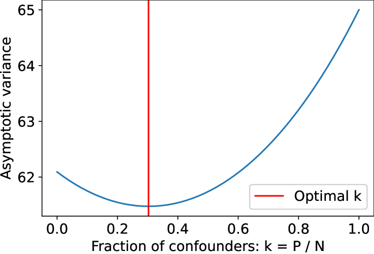
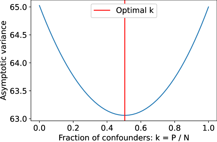
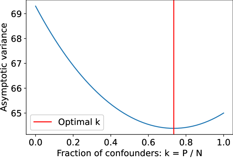
Figure 5 shows three examples where the optimal value of $k$ is between $0$ and $1$. We plot the variance as predicted by the expression for $V_{e}$ versus the value of $k$. The plots show that in some cases, it is better to collect a mix of confounders and mediators rather than only mediators or only confounders. The expression for $V_{e}$ in the previous section allows us to verify that. This happens when the variance of the frontdoor and backdoor estimators do not differ by too much.

In Figure 5(a), the model parameters are $\{a=10,b=3.7,c=5,d=5,\sigma^{2}_{u_{w}}=1,\sigma^{2}_{u_{x}}=1,\sigma^{2}_{u_{m}}=0.64,\sigma^{2}_{u_{y}}=1\}$. In this case, the variance of the frontdoor estimator is lower than the backdoor estimator. Despite this, it is not optimal to only collect mediators. The optimal value of $k$ is $0.303$, that is, $30\%$ of the collected samples should be confounders and the rest should be mediators to achieve lowest variance.

In Figure 5(b), the model parameters are $\{a=10,b=3.955,c=5,d=5,\sigma^{2}_{u_{w}}=1,\sigma^{2}_{u_{x}}=1,\sigma^{2}_{u_{m}}=0.64,\sigma^{2}_{u_{y}}=1\}$. In this case, the variance of the frontdoor estimator is almost equal to that of the backdoor estimator. The optimal ratio $k$ is $0.505$, that is, we should collect the same of amount of confounders as mediators.

In Figure 5(c), the model parameters are $\{a=10,b=4.3,c=5,d=5,\sigma^{2}_{u_{w}}=1,\sigma^{2}_{u_{x}}=1,\sigma^{2}_{u_{m}}=0.64,\sigma^{2}_{u_{y}}=1\}$. In this case, the variance of the frontdoor estimator is greater than the backdoor estimator. The optimal ratio $k$ is $0.735$, that is, we should collect the more confounders than mediators.

F.3 Parameter initialization for finding the MLE

The likelihood in Eq. 6 is non-convex. As a result, we cannot start with arbitrary initial values for model parameters because we might encounter a local minimum. To avoid this, we use the two datasets to initialize our parameter estimates. Each of the eight parameters can be identified using only data from one of the datasets. For example, $d$ can be initialized using the revealed-confounder dataset (via OLS regression of $X$ on $W$). The parameter $e$ is can be identified using either dataset, so we pick the value with lower bootstrapped variance.

After initializing the eight model parameters, we run the Broyden–Fletcher–Goldfarb–Shanno (BFGS) algorithm [Fletcher, 2013] to find model parameters that minimize the negative log-likelihood.

Appendix G More details on experiments

Here we provide more details for how results in Table 1 are generated. We initialize the model parameters by sampling $200$ times from the following distributions:

$$\begin{split}a,b,c,d&\sim\text{Unif}[-10,10]\\ \sigma^{2}_{u_{w}},\sigma^{2}_{u_{x}},\sigma^{2}_{u_{m}},\sigma^{2}_{u_{y}}&\sim\text{Unif}[0.01,2].\end{split}$$ (56)

For each initialization, we compute the Mean Absolute Percentage Error (MAPE) of the theoretical variance as a predictor of empirical variance:

$$\text{MAPE}=\frac{\left|\text{Var}_{\text{theoretical}}-\text{Var}_{\text{empirical}}\right|}{\text{Var}_{\text{empirical}}}*100\%$$

We report the mean and standard deviation of the MAPE across $1000$ realizations of datasets sampled from Eq. 56. We find that the theoretical variance is close to the empirical variance even for small sample sizes (Table 1).

References

- Bareinboim and Pearl [2016] Elias Bareinboim and Judea Pearl. Causal inference and the data-fusion problem. Proceedings of the National Academy of Sciences, 113(27):7345–7352, 2016.
- Bareinboim et al. [2019] Elias Bareinboim et al. Causal inference and data-fusion in econometrics. Technical report, arXiv. org, 2019.
- Bellemare and Bloem [2019] Marc F Bellemare and Jeffrey R Bloem. The paper of how: Estimating treatment effects using the front-door criterion. Working Paper, 2019.
- Chen and Santos [2018] Xiaohong Chen and Andres Santos. Overidentification in regular models. Econometrica, 86(5):1771–1817, 2018.
- Chinco and Mayer [2016] Alex Chinco and Christopher Mayer. Misinformed speculators and mispricing in the housing market. The Review of Financial Studies, 29(2):486–522, 2016.
- Cohen and Malloy [2014] Lauren Cohen and Christopher J Malloy. Friends in high places. American Economic Journal: Economic Policy, 6(3):63–91, 2014.
- Dorie [2016] V. Dorie. Non-parametrics for causal inference. https://github.com/vdorie/npci, 2016.
- Eaton [2007] Morris L. Eaton. Chapter 8: The Wishart Distribution, volume Volume 53 of Lecture Notes–Monograph Series, pages 302–333. Institute of Mathematical Statistics, 2007. 10.1214/lnms/1196285114. URL https://doi.org/10.1214/lnms/1196285114.
- Fletcher [2013] Roger Fletcher. Practical methods of optimization. John Wiley & Sons, 2013.
- Fulcher et al. [2020] Isabel R Fulcher, Ilya Shpitser, Stella Marealle, and Eric J Tchetgen Tchetgen. Robust inference on population indirect causal effects: the generalized front door criterion. Journal of the Royal Statistical Society: Series B (Statistical Methodology), 2020.
- Glynn and Kashin [2017] Adam N Glynn and Konstantin Kashin. Front-door difference-in-differences estimators. American Journal of Political Science, 61(4):989–1002, 2017.
- Glynn and Kashin [2018] Adam N Glynn and Konstantin Kashin. Front-door versus back-door adjustment with unmeasured confounding: Bias formulas for front-door and hybrid adjustments with application to a job training program. Journal of the American Statistical Association, 113(523):1040–1049, 2018.
- Glynn and Kashin [2019] Adam N. Glynn and Konstantin Kashin. Replication Data for: Front-Door Versus Back-Door Adjustment With Unmeasured Confounding: Bias Formulas for Front-Door and Hybrid Adjustments With Application to a Job Training Program, 2019. URL https://doi.org/10.7910/DVN/G7NNUL.
- Hansen [1982] Lars Peter Hansen. Large sample properties of generalized method of moments estimators. Econometrica, 50(4):1029–1054, 1982.
- Henckel et al. [2019] Leonard Henckel, Emilija Perković, and Marloes H Maathuis. Graphical criteria for efficient total effect estimation via adjustment in causal linear models. arXiv preprint arXiv:1907.02435, 2019.
- Hill [2011] Jennifer L Hill. Bayesian nonparametric modeling for causal inference. Journal of Computational and Graphical Statistics, 20(1):217–240, 2011.
- Imbens [2019] Guido Imbens. Potential outcome and directed acyclic graph approaches to causality: Relevance for empirical practice in economics. Technical report, National Bureau of Economic Research, 2019.
- Jackson et al. [2009] CH Jackson, NG Best, and Sylvia Richardson. Bayesian graphical models for regression on multiple data sets with different variables. Biostatistics, 10(2):335–351, 2009.
- Koopmans and Reiersøl [1950] Tjalling C Koopmans and Olav Reiersøl. The identification of structural characteristics. The Annals of Mathematical Statistics, 21(2):165–181, 1950.
- Kuipers and Moffa [2020] Jack Kuipers and Giusi Moffa. The variance of causal effect estimators for binary v-structures. arXiv preprint arXiv:2004.09181, 2020.
- Kuroki [2000] Manabu Kuroki. Selection of post-treatment variables for estimating total effect from empirical research. Journal of the Japan Statistical Society, 2000.
- Pearl [1995] Judea Pearl. Causal diagrams for empirical research. Biometrika, 82(4):669–688, 1995.
- Pearl [2009] Judea Pearl. Causality. Cambridge university press, 2009.
- Pearl [2010] Judea Pearl. The foundations of causal inference. Sociological Methodology, 40(1):75–149, 2010.
- Pearl and Mackenzie [2018] Judea Pearl and Dana Mackenzie. The book of why: the new science of cause and effect. Basic Books, 2018.
- Perković et al. [2015] Emilija Perković, Johannes Textor, Markus Kalisch, and Marloes H Maathuis. A complete generalized adjustment criterion. In Uncertainty in Artificial Intelligence (UAI), 2015.
- Ramsahai [2012] Roland R Ramsahai. Supplementary variables for causal estimation. Wiley Online Library, 2012.
- Rotnitzky and Smucler [2019] Andrea Rotnitzky and Ezequiel Smucler. Efficient adjustment sets for population average treatment effect estimation in non-parametric causal graphical models. arXiv preprint arXiv:1912.00306, 2019.
- Sargan [1958] John D Sargan. The estimation of economic relationships using instrumental variables. Econometrica: Journal of the Econometric Society, pages 393–415, 1958.
- Shalit et al. [2017] Uri Shalit, Fredrik D Johansson, and David Sontag. Estimating individual treatment effect: generalization bounds and algorithms. In International Conference on Machine Learning (ICML), 2017.
- Shi et al. [2019] Claudia Shi, David Blei, and Victor Veitch. Adapting neural networks for the estimation of treatment effects. In Advances in Neural Information Processing Systems, pages 2503–2513, 2019.
- Uhler [2019] C Uhler. Gaussian graphical models: An algebraic and geometric perspective. Chapter in Handbook of Graphical Models, 2019.
- Wright [1934] Sewall Wright. The method of path coefficients. Ann. Math. Statist., 5(3):161–215, 09 1934. 10.1214/aoms/1177732676.