Multivariate Matrix Mittag–Leffler distributions
Abstract.
We extend the construction principle of multivariate phase-type distributions to establish an analytically tractable class of heavy-tailed multivariate random variables whose marginal distributions are of Mittag-Leffler type with arbitrary index of regular variation. The construction can essentially be seen as allowing a scalar parameter to become matrix-valued. The class of distributions is shown to be dense among all multivariate positive random variables and hence provides a versatile candidate for the modelling of heavy-tailed, but tail-independent, risks in various fields of application.
Key words and phrases:
Multivariate distribution; heavy tails; Markov process; Mittag-Leffler distribution; phase-type; matrix distribution; extremes; Laplace transforms1. Introduction
The joint modelling of dependent risks is a crucial task in many areas of applied probability and quantitative risk management, see e.g. McNeil et al., (2015). While in many situations there is a reasonable amount of data available for the fitting procedure of univariate risks, the identification of multivariate models is much more delicate. A frequent approach proposed in applications is to use the available data for univariate fitting, and choose a parametric copula to combine the margins, where the parameters of that copula are then either assumed a priori or estimated from the joint data. The choice of such a copula is of course crucial for the resulting joint distribution and the conclusions one draws from it, cf. Mai and Scherer, (2017); Mikosch, (2006). In multivariate extremes, which is currently a very active research topic, one typically uses less restrictive assumptions for the quantification of joint exceedances, see e.g. Falk et al., (2019); Kiriliouk et al., (2019). Some specific families, like multivariate regular variation, are considered particularly attractive in this context, as they have a natural interpretation in terms of how to extend univariate behaviour into higher dimensions Ho and Dombry, (2019); Joe and Li, (2011); Resnick, (2002). These results focus, however, on the asymptotic behaviour, so that for a concrete application with an available data set one typically has to choose thresholds above which this respective behaviour is assumed Wan and Davis, (2019), and the bulk of the distribution is then to be modelled by a different distribution (see e.g. Beirlant et al., (2004) and (Albrecher et al.,, 2017, Ch.IV.5)).
In this paper we would like to establish a family of multivariate distributions that can be applied for modeling across the entire positive orthant, so that no threshold selection is needed. In particular, we are interested in a family that leads to explicit and tractable expressions for the model fitting and interpretation. While such a family already exists for marginally light (exponentially bounded) tails in the form of multivariate phase-type (MVPH) distributions, our goal here is to develop a related family with heavy-tailed marginal distributions. The univariate starting point for this procedure is the matrix Mittag-Leffler (MML) distribution, which is a heavy-tailed distribution that was recently studied in Albrecher et al., (2019), and which proved to be very tractable, with excellent fitting properties. While in principle there are many possible ways of defining a vector of random variables with given marginals, we want to consider here the natural concept of multivariate families that can be characterized by the property that any linear combination of the components of such a vector is again of the same marginal type. This is exactly one possible definition of MVPH distributions (so any linear combination of the coordinates of a random vector are again (univariate) phase-type), and it is also a characterizing property of multivariate regular variation of a random vector, namely that any linear combination of the coordinates of such a vector is again (univariate) regularly varying, see Basrak et al., (2002).
The goal is hence to study the class of multivariate random vectors for which such a property applies with MML marginal distributions. It will turn out that for this approach to work, we first need to consider a slightly more general class, which we will refer to as generalized MML distributions. We will show that the analysis developed for the MVPH case can then be extended to our more general situation. In particular, we will establish some properties of this class and work out explicit expressions for a number of concrete cases. The analysis is considerably simpler for the symmetric situation where all marginal distributions share the same index of regular variation, but the general case can be handled as well. The resulting multivariate MML distribution is asymptotically independent, i.e. there is tail-independence for each bivariate pair of components. In the case of multivariate regular variation, the subclass of random vectors with asymptotic independence was studied and characterized in terms of second order conditions in Resnick, (2002), where also concrete application areas for such heavy-tailed, but asymptotically independent risks are given. In a sense, the multivariate MML family of distributions we introduce here is another candidate for models in this domain, with the advantage of being explicit and tractable across the entire range . In that respect, this family is also an interesting alternative to multivariate Linnik distributions (see e.g. Anderson, (1992) and Lim and Teo, (2010)), which can be conveniently defined in terms of their characteristic function, have the range (rather than ) and also have heavy-tailed marginals, but which do not lead to explicit expressions for the multivariate density.
The remainder of the paper is organized as follows. Section 2 recapitulates the construction principle of univariate and multivariate PH distributions and provides the available background on MML distributions. Section 3 introduces generalized MML distributions. In Section 4 we then develop the necessary theoretical background for our definition of the multivariate MML family and establish some of its properties. We also consider power transforms, which will provide useful flexibility for modeling applications, and we derive denseness properties of the resulting multivariate family. In Section 5 we work out a concrete simple example in detail and illustrate resulting dependence properties for this case. Section 6 concludes.
2. Phase–type distributions
2.1. Notation
We shall apply a common convention from phase–type theory that matrices are expressed in bold capital letters (e.g. , row vectors are bold minuscular greek letters (e.g. while column vectors are bold minuscular roman letters (e.g. , . Elements of matrices and vectors are denoted by their corresponding minuscular unbold letters with indices, e.g. and . If is a vector, then by we shall denote the diagonal matrix with as diagonal.
2.2. Univariate phase–type distributions
Phase–type distributions are defined as the distribution of the time until absorption of a finite state–space Markov jump process with one absorbing state and the other states being transient.
Let be a positive integer, and denote a Markov jump process on , where states are transient and state is absorbing. Let and assume that , i.e. initiation in the absorbing state is not possible. The intensity matrix of can be written as
| (1) |
where is the sub–intensity matrix whose off diagonal elements consist of transition rates between the transient states, is a –dimensional column vector is a –dimensional row vector. The diagonal elements of are given by , since the row sums of must be zero.
Let denote the vector of ones and . Dimensions are usually suppressed and may then have any adequate dimension depending on the context.
Then the time until absorption,
is said to have a phase–type (PH) distribution with representation and we write . Since rows of sum to zero, we get . Note that the case leads to an exponential distribution.
If , then a number of relevant formulas can be written compactly in matrix notation, like e.g.
for the density, c.d.f., Laplace transform and (fractional) moments, respectively. Here denotes the eigenvalue with maximum real part of , and this real part is strictly negative. In particular, the Laplace transform is well defined for all and in a neighbourhood around zero.
Remark 1.
Representations of phase–type distributions are not unique. In fact, one can construct an infinite number of different representations, which may even be of different orders . Hence phase–type representations may also suffer from over-parametrisation, and it is not possible to attach a specific significance to individual elements of an intensity matrix. While one can typically construct a certain behaviour by means of structuring the sub–intensity matrix , the opposite task of deducing such a behaviour from a given matrix is typically not possible. Some simple cases, however, may be described. For instance, means one phase and the resulting distribution is exponential, hence unimodal. For , bimodality cannot be achieved either, as one could at most aim for a mixture of exponentials. For it is possible to have a mixture of an exponential with an Erlang() which is bimodal.
2.3. Multivariate phase–type distributions
A non–negative random vector is phase–type distributed (MVPH) if all non–negative, non-vanishing linear combinations of its coordinates , have a (univariate) phase–type distribution. This is the most general definition of a multivariate phase–type distribution which, however, lacks practicality since it does not suggest how to construct such distributions. It contains a sub–class of multivariate distributions, MPH∗, which have multidimensional Laplace transforms of the form
| (2) |
and we write that . Here is a phase–type representation of dimension , say, is a matrix and . Furthermore, the joint Laplace transform exists in a neighbourhood around zero ((Bladt and Nielsen,, 2017, Thm.8.1.2)).
The form (2) is established from the following probabilistic construction (cf. Kulkarni, (1989)). Consider the Markov jump process underlying the phase–type distribution with representation . The columns of are –dimensional vectors which contain non–negative numbers. These numbers are “rewards” to be earned during sojourns in state . If denotes the time until absorption of the underlying Markov jump process, then
| (3) |
is the total reward earned according to column of until absorption. The structure matrix hence picks scaled sojourns out of the underlying Markov jump process. Correlation between different total rewards, and say, will then depend on the structure of and on the underlying stochastic process. If there are common states in which reward is earned for both and , then this will contribute to a positive correlation between them. If there are no common states, the correlation will be entirely generated by the structure of the matrix. Negative correlation between and is achieved if large rewards earned in one reduces the one earned in the other and vice versa. Specific constructions of dependencies between Phase–type distributed random variables with given marginals is non–trivial, see. e.g. Bladt and Nielsen, (2010) for an example with exponentially distributed marginals.
The random variables defined in (3) are again phase–type distributed and in general dependent since different variables may be generated through earning positive rewards on certain common states (while in other states there may be zero reward for one variable whenever the other has positive reward). If all , , then is phase–type distributed with initial distribution and sub–intensity matrix . This follows easily from a sample path argument: if reward is earned during a sojourn in state , then the distribution of the reward during a sojourn is exponentially distributed with intensity .
If some , then finding a representation for is more involved. Let denote a non–zero vector. For obtaining the ’th marginal distribution we would choose , the ’th Euclidean unit vector, while for a more general projection we may choose for some constants , . For this given , decompose the set of transient states into , where denotes states for which and states for which . Decompose and
| (4) |
accordingly. Then we have the following theorem which is proved in (Bladt and Nielsen,, 2017, p.441).
Theorem 1.
The distribution of is given by an atom at zero of size and an absolute continuous part given by a possibly defective phase-type distribution with representation , where
This means that
| (5) | |||||
where .
Remark 2.
It is still an open question whether or whether .
Remark 3.
As for univariate phase–type distributions, representations of MPH∗ are not uniquely determined by their distributions, and they may be over–parametrised as well. In particular, the interplay between and introduces further ambiguity.
While both MPH∗ and MPVH distributions lack explicit formulas for distribution and density functions, there is a sub–class of MPH∗ distributions that does allow explicit forms. The latter is the one where the structure of the underlying Markov chain is of so–called feed–forward type.
Let be sub–intensity matrices and let denote non–negative matrices such that . The matrices are not necessarily square matrices, with the number of rows being equal to the number of rows in and the number of columns equal to the number of rows (and columns) of . Define
| (6) |
and let the reward matrix be
| (7) |
The structure of the matrix implies that the ’th total reward, , then equals the inter–arrival time between arrivals and . Positive correlation between two consecutive inter–arrivals and can then be obtained by choosing the matrix in such a way that a long (short) duration of the Markov chain in block will imply a long (short) duration in block as well. For a negative correlation we have to choose the matrix such that the implications are reversed. The joint density of the MPH∗ distribution is then given by
| (8) |
Remark 4.
The matrices are sub–intensity matrices, providing a phase–type distributed time until arrival . The matrices are non–negative matrices containing intensities for initiating a new inter–arrival time for arrival at the time of the arrival . Hence the matrices create the dependence between the inter–arrivals. In particular, if , where is the exit rate (column) vector corresponding to and is some probability (row) vector on , then the inter–arrivals are independent.
Remark 5.
The (full) matrix is not really needed for our purposes, but only the exit vector . Thus we may rewrite (8) in the form
| (9) |
We shall, however, maintain the notation with for notational reasons. Since for all , this also implies the exit vector
so , which is not part of , is part of (see (1)).
Remark 6.
Remark 7.
If and for all , then (8) is the joint density function for the first inter–arrival times of a Markovian Arrival Process (MAP) (see e.g. Neuts, (1979),Bladt and Nielsen, (2017)). This class of point processes is dense in class of point process on (see Asmussen and Koole, (1993)), and therefore the class of distributions given by (8) is also dense – in the sense of weak convergence and with flexible dimension of the matrices and – in the class of multivariate distributions on .
Later we shall need the joint fractional moments for such distributions, which are given in the following lemma.
Lemma 1.
Suppose that has a joint phase–type distribution with density (8). Then for , ,
Proof.
It is sufficient to prove the lemma for .
where is the Laplace transform for . Since the Laplace transforms are analytic (where they are defined), the result follows by a functional calculus argument (see Theorem 3.4.4 of Bladt and Nielsen, (2017)). ∎
2.4. Matrix Mittag–Leffler distributions
Let be a phase–type representation. Then a random variable has a matrix Mittag–Leffler (MML) distribution with representation , if it has Laplace transform
where . We write . Let
denote the Mittag–Leffler (ML) function. Then (see Albrecher et al., (2019)) the density of is given by
and the corresponding c.d.f. is
The ML function with (complex) matrix argument is defined as
For , one can express the (then entire) ML function of a matrix by Cauchy’s formula
where is a simple path enclosing the eigenvalues of . Invoking the residue theorem, for each entry of the matrix , then provides a simple method for calculating .
As outlined in Albrecher et al., (2019), MML distributions with are heavy-tailed with tail indices less than one, so that their mean does not exist. This may be too restrictive in many situations, and one way to obtain a closely related class of distributions is by considering power transformations of the original MML distributed random variables. Indeed, if , then has density
and distribution function
for (cf. Albrecher et al., (2019)). Rewriting leads to the reparametrization
| (10) |
and
| (11) |
Thus, for any and , (10) and (11) define densities and their corresponding distribution functions, with tail index instead of . We shall refer to distributions with densities of the form (10) as power MML and write . Their Laplace transforms are somewhat more involved. Indeed, the Laplace transform for is given by (see formula (5.1.30) in Gorenflo et al., (2014) and compare to (Gorenflo et al.,, 2014, p.364))
3. Generalized matrix Mittag–Leffler distributions
The convolution of Mittag–Leffler distributions is not a Mittag–Leffler distribution. However, if the components in the convolution have the same tail index, then the resulting distribution is a MML.
Theorem 2.
Suppose that and . Then
with
Proof.
This result follows from the Laplace transform of being
∎
Since implies that for any constant , where
we conclude that if are independent MML with the same tail index , then any linear combination with is again MML with tail index .
The convolution of MML distributions with different tail indices are not MML distributions, but naturally lead to an extended class of MML distributions which we refer to as Generalized MML, as we will define in the sequel. If and with , then calculations similar to the proof of Theorem 2 lead to having Laplace transform
| (14) |
where denotes the block diagonal matrix
for square matrices and . The linear combination will then have a Laplace transform on the form,
This motivates the following definition.
Definition 1.
A random variable is said to have a (univariate) generalized matrix Mittag–Leffler distribution, if there exist with , and a phase–type representation for which the absolutely continuous part of its Laplace transform is given by
where are identity matrices and . We write
where .
Then, if are independent with
we get
where
and
By scaling, any non–negative non–zero linear combination of GMML distributed random variables will again follow a GMML distribution.
4. The multivariate matrix Mittag–Leffler distribution
Motivated by Section 3, we proceed now to define the multivariate MML in a similar way as their underlying multivariate phase–type distributions.
Definition 2.
A random vector has a multivariate GMML distribution in the wide sense, if all non–negative non–vanishing linear combinations have a GMML distribution.
As for MVPH distributions, this definition is not very practical from a constructive point of view, and we shall introduce a subclass inspired by (2). To this end we first notice the following result.
Lemma 2.
Let be a multidimensional Laplace transform and let denote functions for which are completely monotone. Then it follows that
is again a Laplace transform.
Proof.
This follows immediately from the multidimensional Bernstein–Widder theorem, see (Bochner,, 2005, p.87), which states that a multivariate function is a multidimensional Laplace transform if and only if it is infinitely often differentiable and
for all . ∎
From this we immediately get the following important result.
Theorem 3.
Let be a representation for a multivariate PH distribution (2). Then the multidimensional function
| (15) |
with , is a multidimensional Laplace transform.
From Theorem 1 we now obtain the following.
Theorem 4.
Proof.
The result follows from
∎
For possibly distinct , we proceed as follows.
Theorem 5.
Proof.
We have that
where . Now splitting into blocks according to and , we see that
where
Then
Now inserting
we get
with
∎
From the previous results we see that we have found a sub-class of multivariate matrix Mittag–Leffler distributions with explicit Laplace transform. This allows us to concentrate on this class, and to make the following definition.
Definition 3.
Let be a random vector. Then we say that has a multivariate matrix generalized Mittag–Leffler distribution if it has joint Laplace transform given by (15), and write
The following result generalizes Theorem 3.6 of Albrecher et al., (2019) to the multivariate case. In particular, it gives the probabilistic interpretation of the GMML class as a family of random vectors whose marginals are absorption times of randomly-scaled, time-inhomogeneous Markov processes. The dependence of the corresponding Markov processes arises from the fact that they are all generated according to a reward structure on an underlying common Markov jump process.
Theorem 6.
Let . Then
| (16) |
where with (see (2)), and where is a vector of independent stable random variables, each with Laplace transform . Here, refers to component-wise multiplication of vectors.
Proof.
We observe that
which implies the desired representation. ∎
Remark 8.
From representation (16), we have that the marginals of any multivariate GMML distribution are regularly varying with indices , all smaller than 1. Moreover, by the multivariate version of Breiman’s lemma (cf. Basrak et al., (2002)) and the fact that multivariate phase–type distributions have moments of all orders, it follows that the tail independence structure of the vector carries over to . That is, the multivariate GMML family introduced in this paper has (very) heavy-tailed GMML marginals, but is tail-independent. As mentioned in the introduction, application areas for such models are e.g. given in Resnick, (2002).
A consequence of is that the mean does not exist. To alleviate this potential practical drawback, it was proposed in Albrecher et al., (2019) to consider power-transformed variables in the univariate case. In the same way, we propose the following definition.
Definition 4.
Let . For , we define
and refer to it as the class of power multivariate MML distributions.
Under the power transform, the class is in general no longer closed under linear combinations. For fixed , however, it possesses the following denseness property (in contrast to distributions with Laplace transform (15)). Here ‘dense on ’ means dense in the sense of weak convergence among all distributions on .
Theorem 7.
(i) The class of variables is dense on .
(ii) For any fixed , the class of variables is dense on .
(iii) For any fixed marginal tail indices , the class of
variables is dense on .
Proof.
(i) The statement is evident by noticing that we may choose and recalling that the class of variables with Laplace transform (2) is dense on .
(ii) Let be any increasing and (entry-wise) diverging sequence of vectors and be an arbitrary random vector on . Let be as in Theorem 6 and notice that . In particular . Moreover, we may choose an independent sequence of vectors with Laplace transforms of the form (2) such that . Applying the continuous mapping theorem, and by the characterization of Theorem 6, the statement follows.
Remark 9.
The above result shows how several classes of multivariate Mittag-Leffler distributions and their power transforms are dense in the set of all distributions of the -dimensional positive orthant. However, since we are dealing with a tail-independent model, the number of phases increases drastically when faced with the need to capture dependence above high thresholds. Heuristically, the tail dependence is only correctly modelled in the limit. This is in some way analogous to the fact that phase–type distributions are dense on all distributions on the positive real line, but they are all light-tailed (of exponential decay), and very large dimensions are needed for approximations of heavy-tailed distributions, cf. Bladt and Nielsen, (2017).
5. Special structures and examples
From the previous sections, it becomes clear that the tail behavior of the GMML class is determined by the parameters (cf. Remark 8) and the dependence structure is mainly triggered by the parameters of the reward matrix , as these determine joint contributions to the size of each component. The marginal behavior and overall shape in the body of the distribution is then finally implied by the structure of the phase-type components (). In particular, the dimension of the latter also determines the potential for possible multimodalities of the components.
In fact, Theorem 7 on the denseness of distributions on relies (implicitly in part (i)) on the possibility of having arbitrarily large dimension , a flexibility that is needed for modelling multiple modes, as the latter can require many phases. However, due to the possibly complex interaction of all parameters, one can not uniquely assign the role of each of the parameters to achieve a particular distributional behavior or shape. Moreover, for arbitrary combinations of parameters it is not always possible to get an explicit expression for the density of a GMML distribution (a complication inherited from the phase-type distributions).
We now proceed to give an example of a subclass that, however, does allow an explicit form. To that end, consider the special structure (6) and (7) for , which in the exponential case led to the density (8),
This choice of , when plugged into (15), results in the joint Laplace transform of
| (17) |
where we now use the shorthand notation . For the resulting class of GMML distributions we can derive joint and marginal density functions, but first we notice the following lemma.
Lemma 3.
Proof.
Since is an analytic function, and a density as a function of , we get that
∎
Remark 10.
The matrix is the so–called Green matrix which has the following probabilistic interpretation: The element of is the expected time that the Markov jump process underlying a phase–type distribution with generator spends in state (prior to absorption) given that it starts in state .
The main result of this section is as follows.
Theorem 8.
The Laplace transform (17) can equivalently be written as
| (18) |
The corresponding joint density is given by
| (19) |
For the ’th marginal distribution of we have
where
Proof.
It is sufficient to prove the result for . (18) follows from the general block diagonal inversion formula
Concerning (19), we have that
which is of the form (15).
The result on the marginal distributions follow from Lemma 3 and by using that , implying that . ∎
The previous result can be used in the construction of bivariate (or multivariate) Mittag–Leffler distributions of a reasonably general type.
Example 1 (Bivariate Mittag–Leffler distribution).
In this example we construct a class of bivariate distributions with Mittag–Leffler distributed marginals. The starting point is the construction of a bivariate exponential distribution underlying the MML. For details on this construction we refer to Section 8.3.2 of Bladt and Nielsen, (2017). Let be a positive integer and
Then for any initial distribution , the phase–type distribution is simply an exponential distribution with intensity . Similarly, if we let
and , then is again exponentially distributed with intensity . Let be a doubly stochastic matrix, i.e. its elements are non–negative and
and define
Consider the reward matrix
Then is a bivariate exponential distribution. This class of bivariate exponential distributions is capable of achieving any feasible correlation (ranging from to ) by choosing sufficiently large and adequately (see Bladt and Nielsen, (2010)). Independence is achieved for
where is the matrix of ones, maximum negative (minimum) correlation (up to order ) by
and maximum positive correlation for order up to by
which is the anti–diagonal unit matrix, cf. He et al., (2012).
The correponding then has a density of the form
| (20) |
where as usual denotes the ’th Euclidian unit vector. The marginals are Mittag–Leffler distributions with densities
for , which follows directly from the invariance under different representations (parametrisations), or by simple integration and using Lemma 3. Note that the present dependence structure has a very natural interpretation as a copula constructed in terms of combining marginal order statistics, cf. Baker, (2008) and (Bladt and Nielsen,, 2017, Sec.8.3.2), here for Mittag-Leffler marginals.
We can write the expression (20) slightly more explicit. The eigenvalues of are , ,…, . To the eigenvalue there corresponds an eigenvector with
Similarly, has eigenvalues and to the eigenvalue there corresponds an eigenvector with
Considering and as column vectors, we form the matrices and . Then we may write
Though the correlation between the Mittag–Leffler marginals is not defined (since moments of orders larger than do not exist), some notion of dependence may be appreciated from the correlation structure of the underlying phase–type distribution.
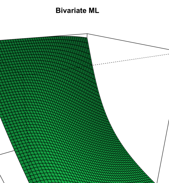
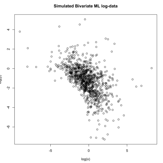
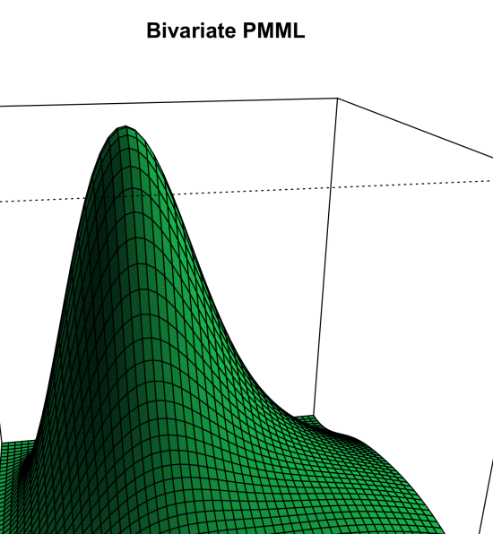
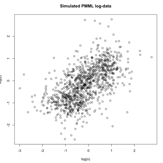
In Figure 1 we depict a bivariate Mittag-Leffler density along with simulated data for the parameters , , , , and the identity matrix.
In Figure 2 we use the same parameters but with being the counter-identity matrix. As expected, the sign of the log-correlation is determined by the structure of the latter matrix. Notice that the number of effective parameters corresponding to each of the two proposed structures is five.
∎
Concerning the power MML with this structure we have the following result.
Theorem 9.
Proof.
Example 2.
Consider the case of a bivariate MML distribution, , and that and have the same dimension (the latter can always be achieved by augmenting the smaller one). Using the abbreviation
we get
If we can calculate variances and correlation. Indeed, with
one has
from which the correlation coefficient is readily calculated.
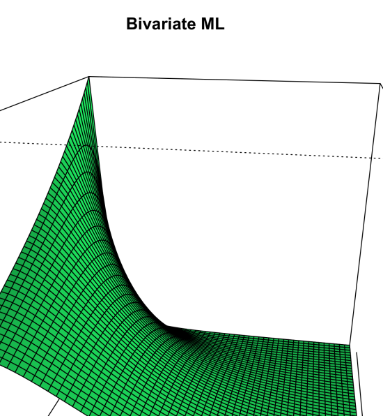
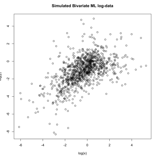
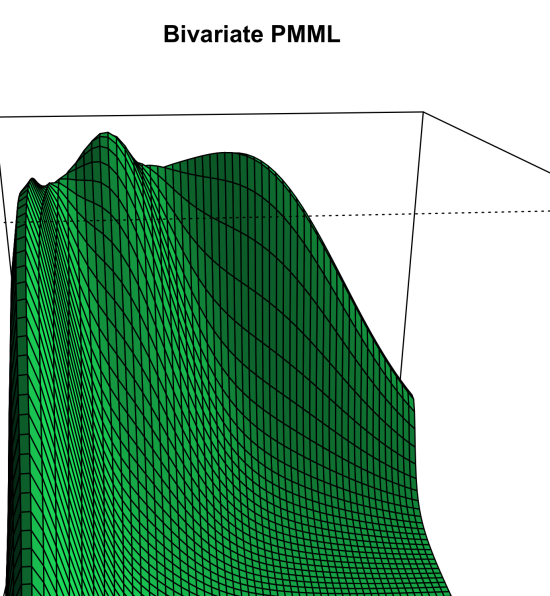
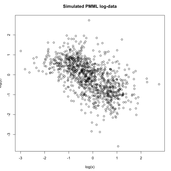
In Figure 3 we depict a bivariate density from a distribution along with simulated data. The parameters are given by
and the phase-type component being of the feed-forward structure (6) and (7), with , , ,
Hence both marginals are mixtures of power Mittag–Leffler distributions. The mixing probabilities of the two distributions are also the same, , since the diagonal form of ensures that the second mixture draws the same component as the first. The first marginal mixture distribution has a density given by
| (21) |
where and , while the second marginal density has the form
| (22) |
The reward matrix is
and and simply correspond to the aforementioned mixtures. The structure of implies a strong positive correlation. For example, if is picked from the mixture component with rate , then will be picked from the same component (but then drawn independently).
In Figure 4 we use the same parameters, except for
Here the correlation between and will be negative: if is drawn from the component with rate , then will be drawn from a component with rate , . The marginal distributions are again given by (21) and (22) since the mixing probabilities are all equal. We observe how the sign of the correlation is affected by the structure of the matrix , and the fact that the matrices are no longer of Erlang structure, the effect is qualitatively opposite to that of the bivariate ML case. One also sees that the class provides quite some flexibility in terms of the shape of the joint density function.
Remark 11.
Dependence may often be constructed by introducing certain structures into the intensity matrices like in Example 1. More generally, dependence between several random variables of MPH∗ type may be constructed using the so–called Baker copula (Baker, (2008)), where order statistics are used and any feasible correlation structure can be obtained.
6. Conclusion
This paper introduces a class GMML of multivariate distributions with matrix Mittag-Leffler distributed marginals. With a construction essentially based on the multivariate phase–type distribution, the GMML class remains a flexible and tractable dense class of distributions maintaining a number of closed form properties. Two important sub–classes are considered, which lead to explicit formulas for distributional properties such as densities and fractional moments. This makes it an attractive candidate for the modelling of both theoretical and practical aspects of multivariate heavy-tailed risks, in situations with tail-independence. The present construction can not be extended to tail-dependent scenarios, so that other approaches will be needed for the latter, which will be an interesting topic for future research.
References
- Albrecher et al., (2017) Albrecher, H., Beirlant, J., and Teugels, J. L. (2017). Reinsurance: Actuarial and Statistical Aspects. John Wiley & Sons, Chichester.
- Albrecher et al., (2019) Albrecher, H., Bladt, M., and Bladt, M. (2019). Matrix Mittag–Leffler distributions and modeling heavy-tailed risks. arXiv preprint arXiv:1906.05316.
- Anderson, (1992) Anderson, D. N. (1992). A multivariate Linnik distribution. Statistics & Probability Letters, 14(4):333–336.
- Asmussen and Koole, (1993) Asmussen, S. and Koole, G. (1993). Marked point processes as limits of Markovian arrival streams. Journal of Applied Probability, 30(2):365–372.
- Baker, (2008) Baker, R. (2008). An order-statistics-based method for constructing multivariate distributions with fixed marginals. Journal of Multivariate Analysis, 99(10):2312–2327.
- Basrak et al., (2002) Basrak, B., Davis, R. A., and Mikosch, T. (2002). A characterization of multivariate regular variation. The Annals of Applied Probability, 12(3):908–920.
- Beirlant et al., (2004) Beirlant, J., Goegebeur, Y., Segers, J., and Teugels, J. L. (2004). Statistics of extremes: theory and applications. John Wiley & Sons, Chichester.
- Bladt and Nielsen, (2010) Bladt, M. and Nielsen, B. F. (2010). On the construction of bivariate exponential distributions with an arbitrary correlation coefficient. Stochastic Models, 26(2):295–308.
- Bladt and Nielsen, (2017) Bladt, M. and Nielsen, B. F. (2017). Matrix-Exponential Distributions in Applied Probability. Springer, Berlin.
- Bochner, (2005) Bochner, S. (2005). Harmonic analysis and the theory of probability. Dover Publications, New York.
- Falk et al., (2019) Falk, M., Padoan, S. A., and Wisheckel, F. (2019). Generalized Pareto copulas: A key to multivariate extremes. Journal of Multivariate Analysis, 174(104538):17 pp.
- Gorenflo et al., (2014) Gorenflo, R., Kilbas, A. A., Mainardi, F., and Rogosin, S. V. (2014). Mittag-Leffler functions, related topics and applications. Springer Monographs in Mathematics. Springer, Berlin.
- He et al., (2012) He, Q.-M., Zhang, H., and Vera, J. C. (2012). On some properties of bivariate exponential distributions. Stochastic Models, 28(2):187–206.
- Ho and Dombry, (2019) Ho, Z. W. O. and Dombry, C. (2019). Simple models for multivariate regular variation and the Hüsler-Reiß Pareto distribution. Journal of Multivariate Analysis, 173:525–550.
- Joe and Li, (2011) Joe, H. and Li, H. (2011). Tail risk of multivariate regular variation. Methodology and Computing in Applied Probability, 13(4):671–693.
- Kiriliouk et al., (2019) Kiriliouk, A., Rootzén, H., Segers, J., and Wadsworth, J. L. (2019). Peaks over thresholds modeling with multivariate generalized Pareto distributions. Technometrics, 61(1):123–135.
- Kulkarni, (1989) Kulkarni, V. G. (1989). A new class of Multivariate Phase type distributions. Operations Research, 37:151–158.
- Lim and Teo, (2010) Lim, S. C. and Teo, L. P. (2010). Analytic and asymptotic properties of multivariate generalized Linnik’s probability densities. The Journal of Fourier Analysis and Applications, 16(5):715–747.
- Mai and Scherer, (2017) Mai, J.-F. and Scherer, M. (2017). Simulating copulas, volume 6 of Series in Quantitative Finance. World Scientific Publishing Co. Pte. Ltd., Hackensack, NJ.
- McNeil et al., (2015) McNeil, A. J., Frey, R., and Embrechts, P. (2015). Quantitative risk management. Princeton Series in Finance. Princeton University Press, Princeton, NJ, revised edition.
- Mikosch, (2006) Mikosch, T. (2006). Copulas: tales and facts. Extremes, 9(1):3–20.
- Neuts, (1979) Neuts, M. (1979). A versatile Markovian point process. Journal of Applied Probability, 16(4):764–779.
- Resnick, (2002) Resnick, S. (2002). Hidden regular variation, second order regular variation and asymptotic independence. Extremes, 5(4):303–336.
- Wan and Davis, (2019) Wan, P. and Davis, R. A. (2019). Threshold selection for multivariate heavy-tailed data. Extremes, 22(1):131–166.