Complexity of Shapes Embedded in with a Bias Towards Squares
Abstract
Shape complexity is a hard-to-quantify quality, mainly due to its relative nature. Biased by Euclidean thinking, circles are commonly considered as the simplest. However, their constructions as digital images are only approximations to the ideal form. Consequently, complexity orders computed in reference to circle are unstable. Unlike circles which lose their circleness in digital images, squares retain their qualities. Hence, we consider squares (hypercubes in ) to be the simplest shapes relative to which complexity orders are constructed. Using the connection between norm and squares we effectively encode squareness-adapted simplification through which we obtain multi-scale complexity measure, where scale determines the level of interest to the boundary. The emergent scale above which the effect of a boundary feature (appendage) disappears is related to the ratio of the contacting width of the appendage to that of the main body. We discuss what zero complexity implies in terms of information repetition and constructibility and what kind of shapes in addition to squares have zero complexity.
Keywords ARS-RBS Morphological analysis methods Shape models and metrics TEC-PDE Partial Differential Equation Based Processing, Level set methods OTH-EMR Complexity TEC-FIL Nonlinear Filtering TEC-FOR Reconstructibility
1 Introduction
Quantifying shape complexity is a classical yet unsolved problem. The key source of difficulty is that complexity is a relative concept. In general, for a given object, the complexity has to do with how it is of interest and what tools are available to describe it (i.e. it is easier to construct a circle if compasses are available, or a triangle if rulers are available).
In the vast majority of the works in the literature, it is assumed that circles are the simplest shapes. The geometric definition and properties of circle bring forth a strong motivation for it to be considered as the simplest. In Euclidean space, one number (radius) is sufficient to construct a circle. However, the property that each point of the circle being equidistant to an enclosed center as measured under the Euclidean metric is not satisfiable in digital spaces. Hence, identifying geometric notions of circularity such as uniform curvature or minimal perimeter per area do not extend when circles are represented as digital images [1], i.e., as subsets of . In this sense, circles lose their circle-ness. Consequently, any measurement obtained by taking circle or circularity as reference is inherently unstable.
In , unlike circles which lose their circle-ness, rectangles with sides parallel to grid axes do not lose their rectangle-ness. An approximation of such a rectangle is still a rectangle; though, it may not be the same one because the aspect ratio of the approximated rectangle may be distorted. Nonetheless, rectangle-ness is unharmed. Of specific interest among rectangles is the one with unit aspect ratio namely square, for it also preserves its unit aspect ratio under approximations. While circles satisfy the property of being equidistant to an enclosed center as measured under Euclidean metric, squares satisfy the same property under metric. The arguments can be extended to arbitrary dimensional shapes. Therefore, we formulate our shape complexity measure with the bias that hypersquares are the simplest shapes by choosing as the right space to measure interactions among a digital shape’s atomic elements, pixels.
Any shape complexity measure should be multi-scale. This is important because a given shape data may contain noise or a shape may have features that are only meaningful at certain scales. Hence, a key ingredient of any shape complexity measurement method is a coarsening process. For the consistency and robustness of the complexity measure, the coarsening process should be suitable with the chosen metric space, meaning that shapes are expected to flow towards the simplest shapes that can be constructed in the chosen space. This is the main drive behind our constructions which use space to construct functions that represent gradual coarsening of the shape boundary. In our multi-scale framework, the scale interval can be sampled up to a number of discrete scale intervals not exceeding the shape width as measured in . At coarser scales, the sensitivity to boundary details is lost causing different shapes (or shapes with different noise levels) to converge in complexity. Indeed, in our method, a cutoff scale emerges such that above it the effect of an appendage (boundary noise or detail) disappears. For rectangular compositions, this cutoff scale is related to the ratio of the contacting width of the appendage to the width of the main body (§ 3.2). Furthermore, when integrated over low-, high-, or all- scales, the proposed complexity measure yields multi-indicators that can be used to construct partial orders if the relationships are too complex to be explained by linear order.
The proposed complexity measure attains absolute zero for shapes in a non-trivial equivalence class including square. This equivalence class, which emerges as a consequence of our constructions, makes compositionality explicit. To exemplify, the measure attains absolute zero for certain square tiles obtained by translating the largest possible base square in the direction of two grid axes (§4). For such square tiles, the size of the largest square that fits the shape is constant at every pixel. That is, the proposed complexity measure respects information repetition. Roughly speaking, a member of the zero-complexity class is maximally compressible and constructible. Additionally, if the measure is used as a guide in an application, such as image segmentation, shape optimization or compression, preference may be steered towards the nearest member(s) of the zero-complexity equivalence class rather than a simple square.
Recently, Fatemi et al. [2] studied recovering binary shape from its sampled representations such that the constructed image is constrained to regenerate the same representations. A more recent work addressing shape from samples is Razavikia et al. [3]. In this context, proposed shape complexity measure can be utilized as a guide for judging how difficult the reconstruction of a shape is.
A different but related problem of recent interest is quantifying the complexity of high-dimensional datasets for estimating their classification difficulty. In that context, a growing number of works emphasize the role of the shape of the decision hyper-surface as a determinant of either how complex the data is [4] or how robust its classification by a certain classifier [5]. As another work in classification context, Varshney and Willsky [6] measured their classifiers in terms of levelsets of the decision hypersurfaces geometrical complexity using -entropy. It appears that measuring high-dimensional shapes is of importance in understanding classifiers and large scale data sets. A particularly interesting claim by Fawzi et al. [5] is that vulnerability to adversarial attacks is related to positive curvature of the decision boundary. Fawzi et al. further attributed the robustness of the popular deep networks to the flatness of the shape of the produced decision boundaries.
2 Literature
Maragos [7] proposed an entropy-like shape-size complexity measure by quantifying the deviation of the shape from a reference shape in a multi-scale way using binary morphological openings and closings with convex structuring elements of increasing sizes. Nguyen and Hoang [8] exploit the properties of Radon transform to measure polygonality. Niimi et al. [9] measured local complexity of bit plane images for data encryption purposes. Gartus and Leder [10] examined the relation between perceived symmetry of abstract binary patterns and computational measures. Fan et al. [11] examined visual complexity of binary ink paintings. Zanette [12] proposed a complexity measure for binary images based on diversity of the length scales in the depicted motifs. The proposed measure penalizes images where gray levels are either distributed at random or ordered into a simple broad pattern. Plotze et al. [13], for the purpose of plant species identification, defined complexity measures of leaf outline and veins. Complexity of binary images and shapes is of wide interest and examples can be enriched.
Page et al. [14] associated shape complexity via entropy of boundary curvature; Chen and Sundaram [15] proposed correlates of Kolmogorov-complexity on boundary curvature, and used them to design efficient shape rejection algorithms [16] that incorporate shape complexity; Chazelle and Incerpi [17] related complexity for polygonal shapes to how entangled the polygon is. Widespread use of boundary-curvature-related information as a correlate of complexity is due to Euclidean geometric consideration of complexity of shapes and seminal perception work [18, 19] that established circle as the simplest. Recently, Genctav and Tari, using curvature-dependent flows, proposed characterizing local circularity [20] and ordered shapes based on entropy in curvature scale space [21].
The earliest interest in quantifying circularity can be traced back to the isoperimetric problem which is the problem of finding which contour, among those of equal perimeters, encloses the maximal area. From this problem follows the form factor, a measure given by for a two dimensional shape of perimeter and area , and is maximized for circles. The form factor and its variants are reviewed by Ritter and Cooper [22]. Rosin proposed several global measures of basic shapes [23, 24].
Measuring rectangularity is emerging as a specific interest due to applications. Urban planning and landscape ecology is one area where rectangular shapes rather than circular ones form a reference [25]. Proper alignment of parts on a robotic production line is another application. In image segmentation applications, rectangularity measure can be used to improve over-segmented images [26]. The need for measuring high dimensional shapes is motivated by understanding large datasets and classifier behavior [6, 5].
3 Method
Using concepts from mathematical morphology (structuring elements, erosions and distance transforms), we make the following observations:
-
•
For a shape , successive upper levelsets of its Euclidean distance transform (EDT) correspond to its successive erosions using a disc structuring element.
-
•
If we shrink the shape boundary by moving its points at a speed proportional to the curvature and in the direction of inward normal, the boundary deforms towards a curve of uniform curvature, i.e., a circle. The regions closed by successive shape boundaries are adaptive erosions and form a multi-scale shape representation.
-
•
If is a circle, i.e, has a uniform boundary curvature, its distance transform’s upper levelsets agree with adaptive erosions. A deviates from a circle, the discrepancy between the respective levelsets increase. The discrepancy is higher for those levelsets that are nearer to boundary and lower for those that are nearer to center.
Suppose we are able to embed boundaries of successive adaptive erosions as levelsets of a field on . Then the congruency between and EDT can be measured by how uniform is at a levelset of of the latter. If is a disc, the levelsets of the two agree. It can be said that the field implicitly encodes curvature [27].
The field construction can be extended to spaces other than Euclidean. In that case, the field may encode some other concept, e.g. of having angles.
Intuitive idea is the following: Circle is the unit ball in Euclidean space. Hence, in Euclidean space, circle is the simplest shape because one parameter (radius) is enough to construct it. Likewise, under the unit ball is the square, which is the ideal shape that can be constructed as a binary image. This motivates us to employ as the proper metric space to implicitly code relevant features.
The proposed method has two components: The first component is to compute in . The second component is to measure how well and the distance transform computed with the right metric agree. In our case, it is , also known as Chebyshev or chessboard distance. In the rest of the paper, will be used to denote the normalized distance transform for a shape.
3.1 Constructing
Assuming the space in which shape is embedded has uniform grid, we solve the following PDE inside
| (1) |
where is the Laplace operator in . We note that is the minimizer of as . Parameter is chosen to be an estimate of the shape radius as measured under . This choice ensures the robustness of solutions under changes in scale. After its construction, is normalized to , which renders the constant on the right hand side of (1) devoid of meaning, so long as the sign is negative. To acquire numerical solutions, the approximation to Laplace operator in [28],
| (2) |
where denotes a unit ball centered at , is used. Note that the expression (2) corresponds to difference between forward and backward morphological derivatives [29, 30].
Points at a system governed by (1) generates and cumulates the values of field. Each point introduces an increment to the neighborhood average (which is in ). Amount of increment is decided by the screening parameter . This increment creates levelsets increasing away from the boundary and these levelsets can be viewed as embeddings of gradual deformations of towards a curve possessing features of the reference shape as determined by the ball of chosen metric space. The maximum value of field is attained at the points with maximum distance to the boundaries, as they are the points of most cumulation.
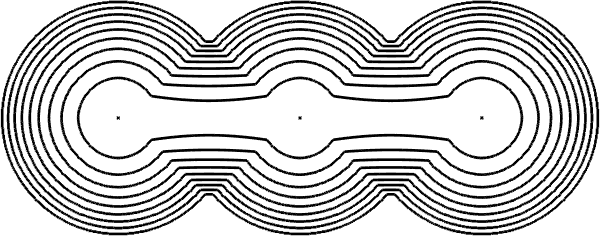
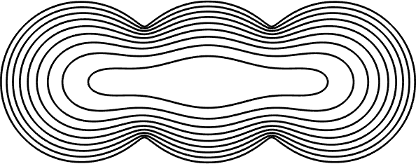
An illustration of the levelsets of (1) is given in Fig. 1 (a). Observe that the level curves become locally flat. For comparison, solution in is depicted in Fig. 1 (b). In the later case, the level sets gets rounder.
 |
 |
| (a) | (b) |
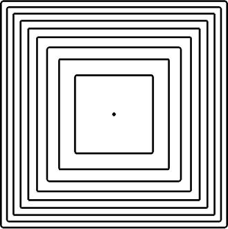
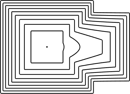
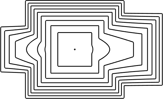
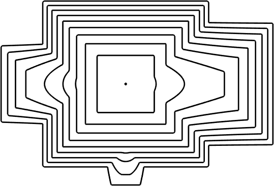
Now let us consider (in setting) the effect of rectangular appendages on the field of a square (Fig. 2). These appendages affect the field only in a region determined by their widths. Outside these regions, they are disregarded. The square has a side length of pixels. The contacting width of the appendages are , , and pixels, respectively.
 |
 |
 |
 |
 |
 |
 |
 |
3.2 Measuring How Well and Agree
The field can be regarded as a well-behaving distance transform. Recall that its levelsets agree with the levelsets of whenever the boundary is isotropic in the sense of chosen metric. The discrepancy between and is due to the smoothed propagation of levelsets of in comparison to those of . To measure discrepancy, it is enough to measure deviation of the values of collected from a level set of from uniformity. Thus, the problem becomes uniformity quantification.
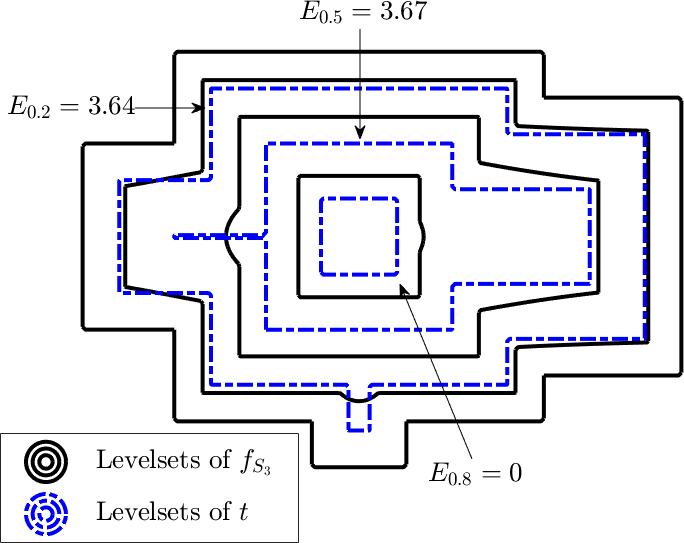
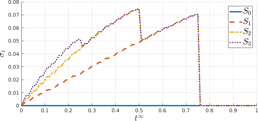
The process is visualized in Fig. 3 using from Fig. 2. The black lines correspond to levelsets of at , , , , and blue dotted lines correspond to those of at , , . is the uniformity estimated at using entropy. To calculate entropy, we need to acquire a pseudo probability distribution. For that purpose, the values of at a levelset of are partitioned into a fixed number of bins (in our implementation, ), and then normalized.
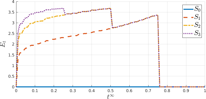
Our intuition is that any uniformity estimator could be used to obtain an ordinal number for complexity. We experimented with both the entropy and standard deviation and observed that their behavior with respect to scale seemed to be equivalent even though their numerical values differ (Fig. 4). In the rest of the paper, to avoid any confusion, we will mean the uniformity estimated using the entropy whenever we refer to shape complexity.
We can talk about a cutoff level of an appendage, such that for effect of the appendage on the field disappears. is determined by the ratio of contacting width of the appendage to the width of the main body. For example, in Fig. 2, for the appendage introduced in is , meaning that for , and are identical. Likewise, for , we have ; and for we have . If we order the four shapes based on the uniformity of the levelsets, the order is for ; for ; for ; finally all shapes become equal after .
 |
 |
Though , it does not define a continuous scale parameter. This is because distance transform produces integer values in . Hence, admits only -many distinct scales.
3.3 Implementation Details
Discretizing (1), we obtain
| (3) |
The field constructed using the explicit scheme
| (4) |
where is the constructed field at the th step, and . Convergence conditions imposed on this scheme are
-
1.
maximum absolute value, , of RHS of (4) is below some threshold, ,
-
2.
In our implementation and are used where is the number of nonzeros of the shape. We can improve this solution by using our insight about the correlation of with the distance transform, and construct a systems based solution. In doing so we use to guide us about the locations of local maxima and minima of the neighborhood of each point.
With this initial guess, we construct where is a sparse matrix and solve for . Pointwise error of the acquired solution is calculated using the LHS of (3), and is fedback to . This process is iterated by using the acquired in the last step as our next guess about the location of local maxima and minima. Convergence condition for the iteration on the systems solution is either having
-
1.
, or
-
2.
.
We used which is greater than since correction of small errors via systems solutions is more costly than correction via the purely iterative scheme. If the iteration on systems solution converged with the second convergence condition, acquired solution is passed to the explicit scheme as the initial condition.
4 Zero-Complexity Shapes
Zero complexity implies that the level sets of and the constructed field are congruent. Consider a shape obtained by adding a rectangular appendage to a base square. If we imagine, at any pixel, comparing the value of to what the value would be if that pixel belonged to a square, the disagreement vanishes after the cutoff scale. If the contacting width is equal to the side length of the square the formed shape becomes a rectangle, making the cutoff scale approach to one and the respective level sets congruent at any scale. We can think of obtaining a rectangle from a base square as translating the center in the direction of the either of the grid axes. Let such that be the side lengths of our rectangle. Consider adding to it a rectangular appendage of height with contacting width of , making either a new rectangle with sides and or compound shape with two rectangles of sizes and . In either of the cases, congruence is unharmed. These are the shapes with constant width and they can be constructed using identical square tiles without losing their qualities. We can also translate the base square in the diagonal direction such that the two squares either overlap or touch. The complexity is zero in either of the cases. This because in the vicinity of the overlap or touch, the configuration is symmetric (in the sense of norm); consequently, level sets of and are congruent. In the case of overlap, a neck joining the two squares is formed; hence, the resulting shape is not of constant width. These shapes attain zero-complexity also in the shape-size complexity framework of Maragos [7], if measured at the scale given by the size of the maximal square. Illustrative examples are depicted in Fig. 5.

A relevant claim by Donderi [31] is that the perceived complexity of a compound shape obtained by overlapping two shapes is the average of their dissimilarity and the average complexity value obtained by averaging perceived complexities of the individual shapes. The behavior of our measure is consistent with this claim. While earlier perception research links perceived complexity to features such as curvature, Donderi [31], Forsythe et al. [32] and several others showed a correlation between compressed-file-size and perceived complexity.
5 Experimental Results and Discussion
In the first experiment, we compare squares and disks with varying sizes. The order shown in Fig. 6 is observed uniformly at all scales. Single arrows are from simpler shapes to more complex ones and double arrows indicate equal complexity. Whenever there is equivalence among a group of shapes, the equivalent shapes are displayed inside a rectangular box. Squares have the lowest (zero) complexity, regardless of their sizes, whereas disks are ordered by increasing size. This is the expected behavior for shapes in . The peak complexity value for the circles is close to , and even for the smallest circle with pixel radius, of the time (scale), the value remains above . In low radius limit, the digital circle becomes a cross hence a zero-complexity shape.

In the second experiment, we compare four rectangular shapes obtained by adding four appendages of widths pixels to a base square with side length pixels.
 |
The ordering at lower scales, , is shown in Fig. 7. As increases beyond the cutoff, , all four shapes attain the same complexity. Any irregularity caused on the field occurs around joints because of the local behavior of solutions. Since the shapes introducing sixteen corners (the last three shapes) cannot be distinguished around joints from one another locally, they have the same complexity. The shape that introduces twelve vertices (the first shape from left), however, can be told apart since it has only four joints, in contrast to eight joints of the other three shapes.
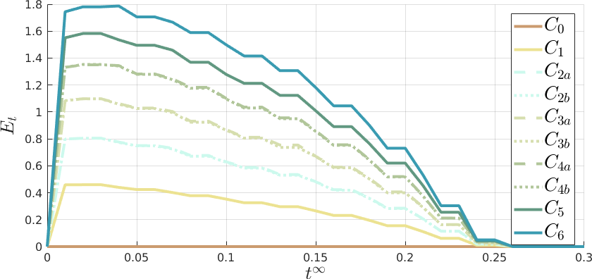
In the third experiment, we construct ten shapes by successively appending smaller cubes of side length voxel at the center of the surfaces of a larger cube of side length voxel. Five samples from the set are depicted in Fig. 8. The naming of the shapes indicate the number of appendages, and their locations, if needed. Subscript indicates a preference towards opposite surfaces when appending a smaller cube, and indicates a preference towards adjacent surfaces.

Scale versus complexity plots in the interval are shown in Fig. 9. is the simplest shape, as expected, with a complexity score of zero uniformly across all values of and the complexity increases with increasing amount of appendages. As the scale increases beyond the cutoff, , all shapes attain zero complexity. These results are in agreement with the results of the two-dimensional shapes.
In the fourth experiment, we observe the joint effect of the placement, size and number of appendages. We construct a set of shapes by varying these three properties. The appendage placement is chosen in two ways: at the center or the corner. The size (width) of appendages is also chosen in two ways: or pixels. Finally, the number of the appendages is chosen in three ways: or . Ordering obtained by our method using values collected at is shown in the top row of Fig. 10. The order is based on the number of appendages first, and between equals, width of appendages is taken into account. That is, it induces a dictionary order. Ordering obtained using values collected at is shown in the bottom row of Fig. 10. All shapes with pixel width appendages attain the same complexity. As increases further, all twelve shapes attain the same complexity.
5.1 Noisy Shapes
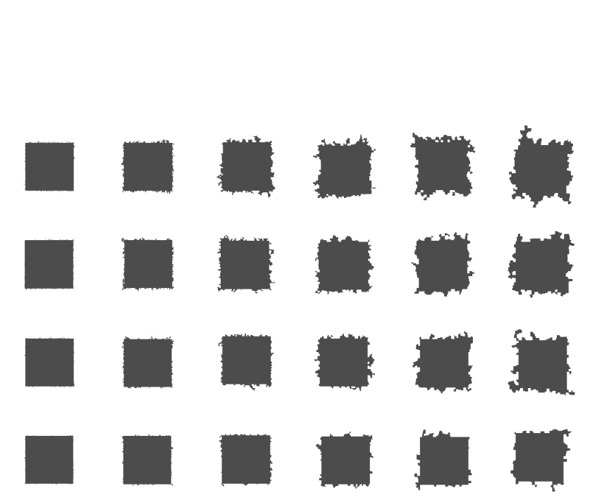
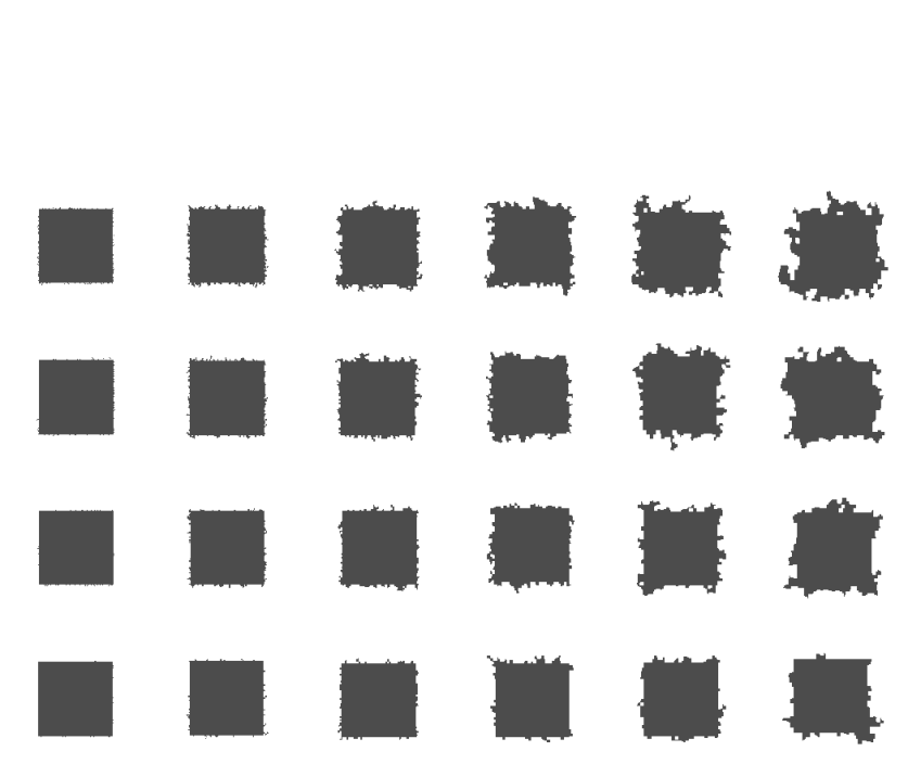
We created fifty random datasets with differing amount of noise
()
and varying noise factors
(),
which results in twenty-four shapes in each of the datasets.
The noise factor determines the width and height of noise stochastically based on the
radius of shape.
Pseudocode addNoise (.) is given in Algorithm. 1.
Two random datasets are shown in Fig. 11.
 |
 |
strel(‘square’, nf)
In the first experiment, we fix the noise factor and then at each noise factor calculate modified Kendall correlation between the expected order (i.e. the order with respect to number of noise applications) and the obtained order. Correlations are calculated for all fifty random datasets. The top four rows of Table 1 show the results for each noise factor. The entries are averaged modified Kendall scores. Respective standard errors of the estimation are depicted in the top four rows of Table 2. We note that the modified Kendall returns for equal pairs regardless of the reference ordering. This is because in this dataset equal complexity values are observed to arise only when the complexity is zero, which means that added noise is completely disregarded.
In the next experiment, we fix the number of noise addition and then at each number calculate modified Kendall correlation between the expected order (i.e. the order with respect to noise factor) and the obtained one. The results are given in the respective bottom four rows of Table 1 and Table 2.
The drop in the scores with increasing and can be explained through the observation that the shapes start to lose their squareness with excessive noise. The agreement between the induced and expected orderings increase with , which is in accordance with the claim that effects of noise are disregarded at higher s.
5.2 Line Drawings of Floor Plans
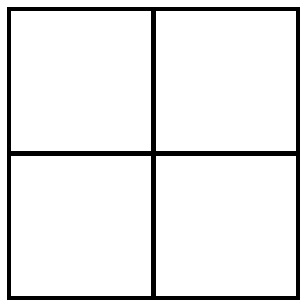
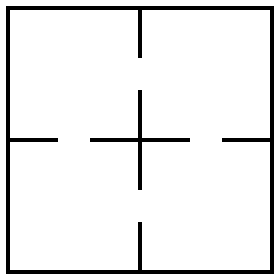
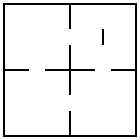
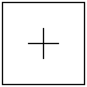
We started with a rectangular drawing of a floor plan and then constructed four simpler cases. All five drawings are displayed in Fig. 12. We inserted them in a frame where lines (shown in black) serve as artificial shape boundaries. The fields and are constructed in the white regions. is a plan of four disconnected identical rooms of side lengths pixels. is constructed by connecting the rooms with apertures of pixels. is constructed by adding an obstacle to one of the rooms aligned with the vertical aperture and of size pixels. is constructed by expanding the length of apertures of to pixel.
 |
 |
 |
 |
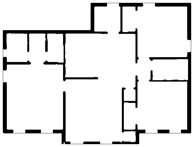 |
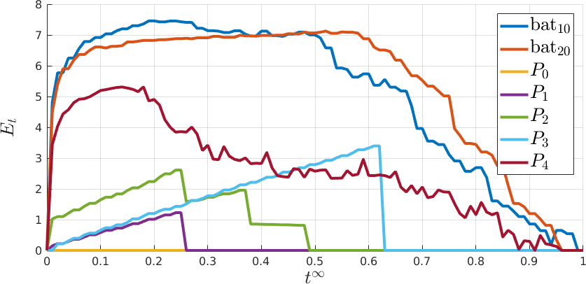
In Fig. 13 scale versus complexity plot for the five line drawings are shown. For comparison, we also include two complex shapes, and (bat silhouettes taken from MPEG7-dataset). The complexity of is higher than that of , , and at all scales, and is lower than that of and at all scales except at where the complexity of is higher than ’s. The complexity of is higher than ’s at and drops to 0 at . This drop is explained by the cutoff level of the apertures of .
5.3 Complex Relations Between Shapes: Incomparable Pairs
As the relation between a pair of shapes gets more complex than adding a rectangular appendage, so does their order relation which no longer exhibits a monotonic behavior with respect to scale. For example, let us compare the complexity of plots of and using Fig. 13. Integrating over all scales in order to obtain single number representing complexity, we can claim that is more complex than . But at lower scales where the boundary features dominate, is simpler than . It is only after a certain scale, when the effect of the obstacle in the upper right room is disregarded, that the order is reversed. There are also other incomparable pairs: and or and . Indeed, it is impossible to linearly order all shapes.
It is, however, of important practical concern to compare shapes based on different complexity considerations. Under such circumstances, although a linear order can not be established on the set of all shapes, it is possible to establish a partial order. Partial order mainly differs from linear order by the presence of incomparable pairs. From a given partial order, subsets on which a linear order is possible -chains- can be extracted. For example, using the measure integrated over low scales, , together with the measure integrated over all scales, yields partial order where and as well as and are incomparable. is the least complex shape.
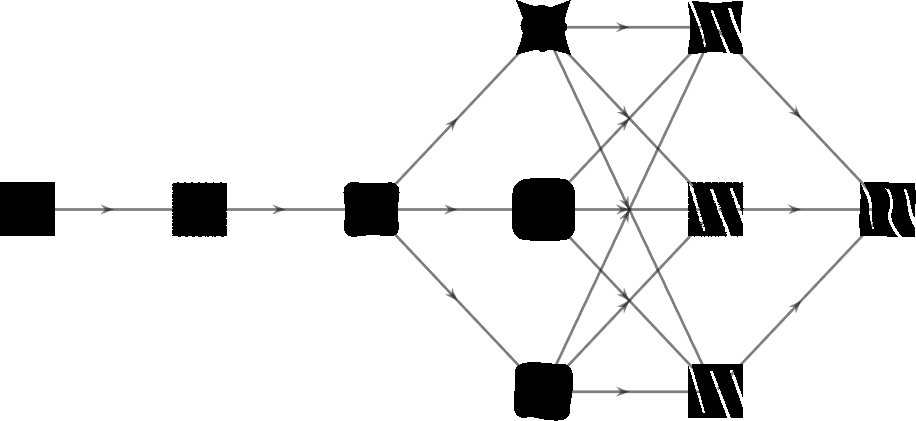
As another example where partial order is more natural than linear order, we considered a set of shapes from device3 category of MPEG7-dataset. Using the same two indicators for measuring complexity (low-scale and all-scale), we constructed a partial order whose graph (Hasse diagram) is depicted in Fig. 14. The first three shapes are ordered linearly based on the deformations of square. The third shape is followed by three others in different branches, each with a different kind of deformation: more concave, more oval, or more curved. All of them are considered less complex than the shapes of the cut group. Among the shapes of the cut group, the most complex is the one with curvy cuts.
6 Summary and Concluding Remarks
Measuring complexity of shapes is important for a variety of reasons. Though the problem is an old one, it lacks robust rigorous solutions because the concept is ill-defined, and biases due to Euclidean geometry are not necessarily useful in digital setting.
We set forth a clear goal in terms of constructibility in digital setting. This motivated us to consider squares (hypercubes in high dimensions) rather than circles as the simplest. Using the link between metric and squares (cubes and hypercubes in higher dimensions) we constructed a field, , whose levelsets encode squareness-adapted multi-scale simplifications. We defined a multi-scale complexity measure by estimating the uniformity of restricted to a certain levelset of . We observed an emergent cutoff scale above which the effect of a boundary detail vanishes. This resulted in different shapes to converge in complexity at higher scales. Furthermore, integrating the complexity over intervals of the scale parameter, we obtained multiple indicators that can be used to construct partial orders.
An interesting future work is to identify local shape elements that increase complexity and suggest a complexity reducing decomposition.
References
- [1] Azriel Rosenfeld. Compact figures in digital pictures. IEEE Transactions on Systems, Man, and Cybernetics, (2):221–223, 1974.
- [2] M. Fatemi, A. Amini, L. Baboulaz, and M. Vetterli. Shapes from pixels. IEEE Transactions on Image Processing, 25(3):1193–1206, 2016.
- [3] S. Razavikia, A. Amini, and S. Daei. Reconstruction of binary shapes from blurred images via hankel-structured low-rank matrix recovery. IEEE Transactions on Image Processing, 2019.
- [4] Tin Kam Ho and M. Basu. Complexity measures of supervised classification problems. IEEE Transactions on Pattern Analysis and Machine Intelligence, 24(3):289–300, 2002.
- [5] A. Fawzi, S. Moosavi-Dezfooli, and P. Frossard. The robustness of deep networks: A geometrical perspective. IEEE Signal Processing Magazine, 34(6):50–62, 2017.
- [6] Kush R. Varshney and Alan S. Willsky. Classification using geometric level sets. J. Mach. Learn. Res., 11:491–516, 2010.
- [7] Petros Maragos. Pattern spectrum and multiscale shape representation. IEEE Transactions on Pattern Analysis and Machine Intelligence, 11(7):701–716, 1989.
- [8] Thanh Phuong Nguyen and Thai V Hoang. Projection-based polygonality measurement. IEEE Transactions on Image Processing, 24(1):305–315, 2014.
- [9] Michiharu Niimi, Hideki Noda, and Eiji Kawaguchi. An image embedding in image by a complexity based region segmentation method. In IEEE International Conference on Image Processing, volume 3, pages 74–77, 1997.
- [10] Andreas Gartus and Helmut Leder. Predicting perceived visual complexity of abstract patterns using computational measures: The influence of mirror symmetry on complexity perception. PloS one, 12(11), 2017.
- [11] Zhen Bao Fan, Yi-Na Li, Jinhui Yu, and Kang Zhang. Visual complexity of chinese ink paintings. In Proceedings of the ACM Symposium on Applied Perception, pages 9:1–9:8, 2017.
- [12] D Zanette. Quantifying the complexity of black-and-white images. PloS one, 13(11), 2018.
- [13] Rodrigo Oliveira Plotze, M Falvo, Juliano Gomes Padua, Luis Carlos Bernacci, Maria Lúcia Carneiro Vieira, Giancarlo Conde Xavier Oliveira, and Odemir Martinez Bruno. Leaf shape analysis using the multiscale minkowski fractal dimension, a new morphometric method: a study with passiflora (passifloraceae). Canadian Journal of Botany, 83(3):287–301, 2005.
- [14] D. L. Page, A. F. Koschan, S. R. Sukumar, B. Roui-Abidi, and M. A. Abidi. Shape analysis algorithm based on information theory. In IEEE International Conference on Image Processing, volume 1, pages 229–232, 2003.
- [15] Y. Chen and H. Sundaram. Estimating complexity of 2d shapes. In IEEE Workshop on Multimedia Signal Processing, pages 1–4, 2005.
- [16] Yinpeng Chen and Hari Sundaram. A computationally efficient 3d shape rejection algorithm. In IEEE International Conference on Multimedia and Expo, pages 4–pp, 2005.
- [17] B. Chazelle and J. Incerpi. Triangulation and shape-complexity. ACM Transactions on Graphics, 3(2):135–152, April 1984.
- [18] Fred Attneave. Physical determinants of the judged complexity of shapes. Journal of Experimental Psychology, 53(4):221, 1957.
- [19] Malcolm D Arnoult. Prediction of perceptual responses from structural characteristics of the stimulus. Perceptual and Motor Skills, 11(3):261–268, 1960.
- [20] Asli Genctav and Sibel Tari. Discrepancy: Local/global shape characterization with a roundness bias. Journal of Mathematical Imaging and Vision, 61(1):160–171, 2019.
- [21] Asli Genctav and Sibel Tari. A product shape congruity measure via entropy in shape scale space. arXiv preprint arXiv:1709.03086, 2017.
- [22] Nicola Ritter and James Cooper. New resolution independent measures of circularity. Journal of Mathematical Imaging and Vision, 35(2):117–127, 2009.
- [23] Paul L Rosin. Measuring rectangularity. Machine Vision and Applications, 11(4):191–196, 1999.
- [24] Paul L Rosin. Measuring shape: ellipticity, rectangularity, and triangularity. Machine Vision and Applications, 14(3):172–184, 2003.
- [25] Dietmar Moser, Harald G Zechmeister, Christoph Plutzar, Norbert Sauberer, Thomas Wrbka, and Georg Grabherr. Landscape patch shape complexity as an effective measure for plant species richness in rural landscapes. Landscape Ecology, 17(7):657–669, 2002.
- [26] Tran-Thanh Ngo, Christophe Collet, and Vincent Mazet. Automatic rectangular building detection from vhr aerial imagery using shadow and image segmentation. In IEEE International Conference on Image Processing, pages 1483–1487, 2015.
- [27] Z Sibel Goktepe Tari, Jayant Shah, and Homer Pien. A computationally efficient shape analysis via level sets. In IEEE Workshop on Mathematical Methods in Biomedical Image Analysis, pages 234–243, 1996.
- [28] Adam Oberman. A convergent difference scheme for the infinity laplacian: construction of absolutely minimizing lipschitz extensions. Mathematics of Computation, 74(251):1217–1230, 2005.
- [29] Petros Maragos. Differential morphology and image processing. IEEE Transactions on Image Processing, 5(6):922–937, 1996.
- [30] Roger W Brockett and Petras Maragos. Evolution equations for continuous-scale morphology. In IEEE International Conference on Acoustics, Speech, and Signal Processing, volume 3, pages 125–128, 1992.
- [31] D. C. Donderi. An information theory analysis of visual complexity and dissimilarity. Perception, 35(6):823–35, 2006.
- [32] A Forsythe, Marcos Nadal, Noel Sheehy, Camilo José Cela-Conde, and Martin Sawey. Predicting beauty: fractal dimension and visual complexity in art. British Journal of Psychology, 102(1):49–70, 2011.