Mix-n-Match: Ensemble and Compositional Methods for Uncertainty Calibration in Deep Learning

Abstract

This paper studies the problem of post-hoc calibration of machine learning classifiers. We introduce the following desiderata for uncertainty calibration: (a) accuracy-preserving, (b) data-efficient, and (c) high expressive power. We show that none of the existing methods satisfy all three requirements, and demonstrate how Mix-n-Match calibration strategies (i.e., ensemble and composition) can help achieve remarkably better data-efficiency and expressive power while provably maintaining the classification accuracy of the original classifier. Mix-n-Match strategies are generic in the sense that they can be used to improve the performance of any off-the-shelf calibrator. We also reveal potential issues in standard evaluation practices. Popular approaches (e.g., histogram-based expected calibration error (ECE)) may provide misleading results especially in small-data regime. Therefore, we propose an alternative data-efficient kernel density-based estimator for a reliable evaluation of the calibration performance and prove its asymptotically unbiasedness and consistency. Our approaches outperform state-of-the-art solutions on both the calibration as well as the evaluation tasks in most of the experimental settings. Our codes are available at https://github.com/zhang64-llnl/Mix-n-Match-Calibration.

1 Introduction

Figure 1: (Top): (left) Temperature Scaling (TS) (Guo et al., 2017) is data-efficient (initial rapid ECE drop) but not expressive (fails to make progress later); in contrast, Isotonic Regression (IR) (Zadrozny & Elkan, 2002) is more expressive but data-inefficient; (right) IR does not preserve accuracy and introduces significant accuracy drop. (Bottom) Mix-n-Match: (left) Data Ensemble and Composition improve the data efficiency of IR, and (right) Model Ensemble enhances the expressive power of TS. All results are for calibrating a 50-layer Wide ResNet on ImageNet, apart from (a) left (28-layer Wide ResNet on CIFAR-10).

Machine learning (ML) models, e.g., deep neural networks, are increasingly used for making potentially important decisions in applications ranging from object detection (Girshick, 2015), autonomous driving (Chen et al., 2015) to medical diagnosis (Litjens et al., 2017). Several of these applications are high-regret in nature and incorrect decisions have significant costs. Therefore, besides achieving high accuracy, it is also crucial to obtain reliable uncertainty estimates, which can help deciding whether the model predictions can be trusted (Jiang et al., 2018; Kendall & Gal, 2017). Specifically, a classifier should provide a calibrated uncertainty measure in addition to its prediction. A classifier is well-calibrated, if the probability associated with the predicted class label matches the probability of such prediction being correct (Bröcker, 2009; Dawid, 1982). Unfortunately, many off-the-shelf ML models are not well calibrated (Niculescu-Mizil & Caruana, 2005; Zadrozny & Elkan, 2001, 2002). Poor-calibration is particularly prominent in highly complex models such as deep neural network classifiers (Guo et al., 2017; Hein et al., 2019; Lakshminarayanan et al., 2017; Nguyen et al., 2015).

A popular calibration approach is to learn a transformation (referred to as a calibration map) of the trained classifier’s predictions on a calibration dataset in a post-hoc manner. Pioneering work along this direction include Platt scaling (Platt, 2000), histogram binning (Zadrozny & Elkan, 2001), isotonic regression (Zadrozny & Elkan, 2002), Bayesian binning into quantiles (Naeini et al., 2015). Recently, calibration methods for multi-class deep neural network classifiers have been developed, which include: temperature, vector & matrix scaling (Guo et al., 2017), Dirichlet scaling (Kull et al., 2019), intra order-preserving method (Rahimi et al., 2020) and Gaussian processes based calibration methods (Milios et al., 2018; Wenger et al., 2020). Besides post-hoc calibrations, there also exist approaches for training ab-initio well calibrated models (Kumar et al., 2018; Lakshminarayanan et al., 2017; Pereyra et al., 2017; Seo et al., 2019; Tran et al., 2019), or representing the prediction uncertainty in a Bayesian framework (Blundell et al., 2015; Gal & Ghahramani, 2016; Maddox et al., 2019).

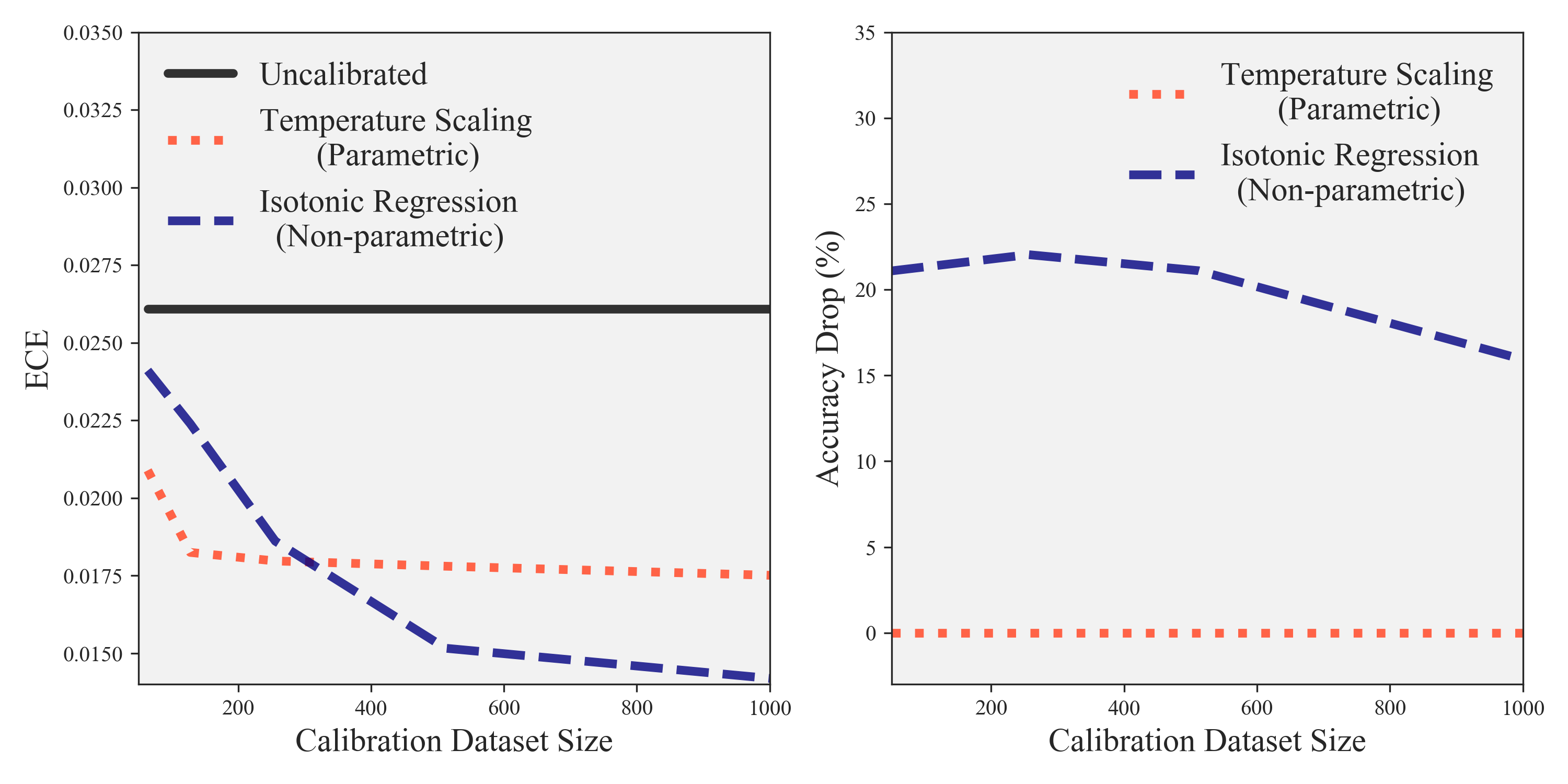
Ideally, an uncertainty calibration method should satisfy the following properties: (a) accuracy-preserving – calibration process should not degrade the classification accuracy of the original classifier, (b) data-efficiency – the ability to achieve well-calibration without requiring a large amount of calibration data, and (c) high expressive power – sufficient representation power to approximate the canonical calibration function given enough calibration data. Despite the popularity of post-hoc calibration, we found that none of the existing methods satisfy all requirements simultaneously (Figure 1). Yet given practical constraints, such as high data collection costs, high complexity of calibration tasks, and need for accurate classifiers, the development of calibration methods which satisfy all three requirements simultaneously is crucial for the success of real-world ML systems.

After calibrating a classifier, the next equally important step is to reliably evaluate the calibration performance. Most of the existing works judge the calibration performance by the expected calibration error (ECE) (Naeini et al., 2015). ECE is usually estimated from a reliability diagram and its associated confidence histogram (Guo et al., 2017; Naeini et al., 2015). However, histogram-based ECE estimators can be unreliable (e.g., asymptotically biased or noisy) due to their sensitivity to binning schemes (Ashukha et al., 2020; Ding et al., 2020; Nixon et al., 2019; Vaicenavicius et al., 2019). Additionally, as a density estimator, histogram is known to be less data-efficient than alternative choices, such as kernel density estimators (Scott, 1992). Therefore, it is of utmost importance to develop reliable and data-efficient methods to evaluate the calibration performance.

To achieve the aforementioned objectives, this paper makes the following contributions:

1. We introduce the following desiderata for uncertainty calibration – (a) accuracy-preserving, (b) data-efficient, and (c) expressive.

2. We propose ensemble and compositional calibration strategies to achieve high data-efficiency and expressive power while provably preserving accuracy.

3. We propose a data-efficient kernel density estimator for a reliable evaluation of the calibration performance.

4. Using extensive experiments, we show that the proposed Mix-n-Match calibration schemes achieve remarkably better data-efficiency and expressivity upon existing methods while provably preserve accuracy.

2 Definitions and Desiderata

Consider a multi-class classification problem. The random variable $X\in\mathcal{X}$ represents the input feature, and $Y=(Y_{1},\ldots,Y_{L})\in\mathcal{Y}$ represents the $L$-class one-hot encoded label. Let $f:\mathcal{X}\rightarrow\mathcal{Z}\subseteq\Delta^{L}$ be a probabilistic classifier that outputs a prediction probability (or confidence) vector $z=f(x)=(f_{1}(x),\ldots,f_{L}(x))$, where $\Delta^{L}$ is the probability simplex $\{(z_{1},\ldots,z_{L})\in[0,1]^{L}|\sum_{l=1}^{L}z_{l}=1\}$. Let $\mathbb{P}(Z,Y)$ denote the joint distribution of the prediction $Z$ and label $Y$. Expectations ($\mathbb{E}$) are taken over this distribution unless otherwise specified. Let the canonical calibration function $\pi(z)$ represents the actual class probability conditioned on the prediction $z$ (Vaicenavicius et al., 2019):

$$\begin{split}\pi(z)&=(\pi_{1}(z),\ldots,\pi_{L}(z))\\ \text{with }&\pi_{l}(z)=\mathbb{P}[Y_{l}=1|f(X)=z].\end{split}$$ (1)

We would like the predictions to be calibrated, which intuitively means that it represents a true probability. The formal definition of calibration is as follows:

Definition 2.1.

The classifier $f$ is perfectly calibrated, if for any input instances $x\in\mathcal{X}$, the prediction and the canonical calibration probabilities match: $z=\pi(z)$ (Dawid, 1982).

We focus on a post-hoc approach for calibrating a pre-trained classifier, which consists of two steps: $(1)$ finding a calibration map $T:\Delta^{L}\rightarrow\Delta^{L}$ that adjusts the output of an existing classifier to be better calibrated, based on a set of $n_{c}$ calibration data samples; and $(2)$ evaluate the calibration performance based on a set of $n_{e}$ evaluation data samples. Next, we discuss both steps in detail and highlight shortcomings of current methods.

2.1 Calibration Step

The first task in the calibration pipeline is to learn a calibration map $T$ based on $n_{c}$ calibration data samples $\{(z^{(i)},y^{(i)})\}_{i=1}^{n_{c}}$. Existing calibration methods can be categorized into two groups:

Parametric methods assume that the calibration map belongs to a finite-dimensional parametric family $\mathcal{T}=\{T(z;\theta)|\theta\in\Theta\ \subseteq\mathbb{R}^{M}\}$. As an example, for binary classification problems, Platt scaling (Platt, 2000) uses the logistic transformation to modify the prediction probability of a class (assuming $z_{1}$): $T(z_{1};a,b)=(1+\exp{(-az_{1}-b)})^{-1}$, where the scalar parameters $a$, $b$ are learned by minimizing the negative log likelihood on the calibration data set. Parametric methods are easily extendable to multi-class problems, such as temperature, matrix scaling (Guo et al., 2017) and Dirichlet scaling (Kull et al., 2019).

Non-parametric methods assume that the calibration map is described with infinite-dimensional parameters. For binary classification problems, popular methods include: histogram binning (Zadrozny & Elkan, 2001) which leverages histograms to estimate the calibration probabilities $\pi(z)$ as the calibrated prediction $T(z)$, Bayesian Binning (Naeini et al., 2015) performs Bayesian averaging to ensemble multiple histogram binning calibration maps, and isotonic regression (Zadrozny & Elkan, 2002) learns a piecewise constant isotonic function that minimizes the residual between the calibrated prediction and the labels. A common way to extend these methods to a multi-class setting is to decompose the problem as $L$ one-versus-all problems (Zadrozny & Elkan, 2002), separately identify the calibration map $T_{l}$ for each class probability ($z_{l}$) in the binary manner, and finally normalize the calibrated predictions into $\Delta^{L}$.

While there are existing approaches tailored for calibrating multi-class deep neural network models, none of them simultaneously satisfy all three proposed desiderata (accuracy-preserving, data-efficient, expressive). Figure 1 (top right) highlights that good calibration capability might come at the cost of classification accuracy for approaches such as isotonic regression. This motivates us to design provably accuracy-preserving calibration methods. Furthermore, the effectiveness of calibration method changes with the amount of calibration data. Parametric approaches are usually data-efficient but have very limited expressive power. On the other hand, non-parametric approaches are expressive but highly data-inefficient. Therefore, in Figure 1 (top left), we see that temperature scaling is the best calibration method in data-limited regime, while isotonic regression is superior in data-rich regime. It is thus naturally desirable to design a calibrator that is effective in both data-limited and data-rich regime. However, earlier studies examined calibration methods with fixed dataset size (Guo et al., 2017; Kull et al., 2019; Wenger et al., 2020), and shed no light on this issue.

2.2 Calibration Error Evaluation Step

The next task in the calibration pipeline is to evaluate the calibration performance based on $n_{e}$ evaluation data points $\{(z^{(i)},y^{(i)})\}_{i=1}^{n_{e}}$. A commonly used statistics is the expected deviation from $z$ to $\pi(z)$, also called expected calibration error (Naeini et al., 2015):

$$\text{ECE}^{d}(f)=\mathbb{E}\lVert Z-\pi(Z)\rVert_{d}^{d}=\int\lVert z-\pi(z)\rVert_{d}^{d}\;p(z)\mathop{dz}$$ (2)

where $\lVert\cdot\rVert_{d}^{d}$ denotes the $d$-th power of the $\ell_{d}$ norm, and $p(z)$ represents the marginal density function of $Z=f(X)$. The original ECE definition adopts $d=1$ (Guo et al., 2017; Naeini et al., 2015), while $d=2$ is also commonly used (Bröcker, 2009; Hendrycks et al., 2019; Kumar et al., 2019).

Note that probabilities in Eq. (1) and Eq. (2) cannot be computed directly using finite samples, since $\pi(z)$ is a continuous random variable. This motivates the need of designing reliable ECE estimators. A popular estimation approach is based on histograms (Naeini et al., 2015). It partitions the evaluation data points into $b$ bins $\{B_{1},\ldots,B_{b}\}$ according to the predictions $z$, calculate the average prediction $\bar{f}(B_{i})$ and label $\bar{\pi}(B_{i})$ inside the bins $B_{i}$, and estimate ECE by:

$$\overline{\text{ECE}}^{d}(f)=\sum_{i=1}^{b}\frac{\#B_{i}}{n_{e}}\lVert\bar{f}(B_{i})-\bar{\pi}(B_{i})\rVert_{d}^{d}.$$ (3)

where $\#B_{i}$ denotes the number of instances in $B_{i}$.

Despite its simplicity, histogram-based estimator suffers from several issues. First, it has bias-variance dilemma with respect to the selection of bin amount and edge locations. For example, too few bins lead to under-estimation of ECE (Kumar et al., 2019), while too many bins leads to noisy estimates as each bin becomes sparsely populated (Ashukha et al., 2020; Ding et al., 2020; Nixon et al., 2019; Vaicenavicius et al., 2019). Therefore, histogram-based ECE estimators are unreliable (e.g., asymptotically biased or noisy) due to their sensitivity to the binning scheme. Unfortunately, a consistently reliable binning selection scheme does not exist (Scott, 1992; Simonoff & Udina, 1997). Finally, histogram-based estimator is known to converge slower than other advanced non-parametric density estimators (Scott, 1992), leading to a data-inefficient estimation of ECE.

Next (in Sec. 3), we discuss the proposed Mix-n-Match calibration strategies which satisfy the above discussed desiderata. Later (in Sec. 4), we will address the issue of designing a reliable and data-efficient ECE estimator.

3 Designing Calibration Methods

We first present (in Sec. 3.1) a general strategy to design provably accuracy-preserving calibration methods. Next, we discuss strategies for parametric (in Sec. 3.2) and non-parametric calibration methods (in Sec. 3.3) to fulfill remaining desiderata.

3.1 Accuracy-preserving Calibration

We present a general form of accuracy-preserving calibration maps and validate its accuracy-preserving property.

Definition 3.1 (Accuracy-Preserving Calibration Map).

Let $g:[0,1]\rightarrow\mathbb{R}_{\geq 0}$ be a non-negative strictly isotonic function. Then, an accuracy-preserving calibration map is given by:

$$T(z)={(g(z_{1}),g(z_{2}),\ldots,g(z_{L}))}/{\sum_{l=1}^{L}g(z_{l})}.$$ (4)

In Eq. (4), we apply the same function $g$ to transform all entries in the prediction probability vector $z$ to an un-normalized vector $g(z)=(g(z_{1}),\ldots,g(z_{L}))$; and normalize $g(z)$ to a probability simplex $\Delta^{L}$. The single strictly isotonic function $g$ maintains the ordering of class prediction probabilities, and preserves the classification accuracy.

Proposition 3.1.

The calibration map in Eq. (4) preserves the classification accuracy of the uncalibrated classifier.

Proof.

Please see supplementary material Sec. A. ∎

3.2 Parametric Calibrations

Parametric methods are already data-efficient, thus, one simply needs to enforce the accuracy-preserving requirement and improve their insufficient expressive power.

3.2.1 Preserving accuracy

As discussed in Proposition 3.1, the use of a strictly isotonic function preserves the accuracy. Fortunately, several existing parametric methods, such as, Platt (Platt, 2000) or temperature scaling (Guo et al., 2017), and beta scaling (Kull et al., 2017), employ strictly isotonic functions – logistic function and beta function, respectively. Therefore, these methods are already accuracy-preserving. Otherwise, the general form as provided in Eq. (4) can be used for designing accuracy-preserving calibration maps.

3.2.2 Improving expressivity by model ensemble

We outline a strategy compatible with any parametric calibration method to improve its expressivity. The idea is to use an ensemble of calibration maps from the same accuracy-preserving parametric family, but with different parameters (see Figure 2):

$$T(z)=w_{1}T(z;\theta_{1})+w_{2}T(z;\theta_{2})+\ldots+w_{M}T(z;\theta_{M}),$$

where $w$ are non-negative coefficients summing up to one. The weighted sum preserves isotonicity, thus the ensemble inherits the accuracy-preserving property from its individual components. The increased expressivity stems from the fact that more parameters becomes adjustable, including $\theta_{j}$ and the weights $w_{j}$ for each component $j$ in the ensemble. We find the weights $w$ and parameters $\theta$ by minimizing the loss $R(.)$ between calibrated predictions $T(z)$ and labels $y$:

$$\underset{w,\theta}{\text{minimize}} \sum_{i=1}^{n_{c}}R\big{(}\sum_{j=1}^{M}w_{j}T(z^{(i)};\theta_{j}),y^{(i)}\big{)}$$

s.t. $$\mathbf{1}_{1\times M}w=1;w\geq\mathbf{0}_{M\times 1}.$$

Figure 2: Model Ensemble calibration for improving expressivity. The idea is to use the weighted averaged outputs of an ensemble of $M$ calibration maps to get the final calibrated prediction. Trainable parameters are highlighted in red.

Using the above formulation, we show a specific generalization of temperature scaling (TS) (Guo et al., 2017) to satisfy the proposed desiderata.

Ensemble Temperature Scaling (ETS). Note that TS is already accuracy-preserving and data-efficient. Next, we propose an ensemble formulation to improve the expressivity of TS while maintaining its accuracy-preserving and data-efficiency properties. Specifically, we propose a three-component ensemble as follows:

$$T(z;w,t)=w_{1}T(z;t)+w_{2}z+w_{3}\frac{1}{L},$$ (5)

where the calibration map for original TS is expressed by $T(z;t)={(z_{1}^{1/t},z_{2}^{1/t},\ldots,z_{L}^{1/t})}/{\sum_{l=1}^{L}z_{l}^{1/t}}$. Interestingly, the remaining two components in the ensemble are also TS calibration maps but with fixed temperature $t$:

• TS calibration map with $t=1$ (outputs uncalibrated prediction $z$). It increases the stability when the original classifier is well calibrated (Kull et al., 2017).

• TS calibration map with $t=\infty$ (outputs uniform prediction $z_{l}=1/L$ for each class). It ‘smooths’ the predictions, similar to how label-smoothing training technique smooths the one-hot labels (Szegedy et al., 2016), which has shown to be successful in training better calibrated neural networks (Müller et al., 2019).

The weight $w$ and temperature $t$ of ensemble is identified by solving the following convex optimization problem:

$$\underset{t,w}{\text{minimize}} \sum_{i=1}^{n_{c}}R\big{(}w_{1}T(z^{(i)};t)+w_{2}z^{(i)}+w_{3}\frac{1}{L},y^{(i)}\big{)}$$

s.t. $$t>0;\mathbf{1}_{1\times 3}w=1;w\geq\mathbf{0}_{3\times 1}.$$

ETS preserves the accuracy, as it uses a convex combination of (strictly) isotonic function $g=z_{l}^{1/t}$ across all classes/components. Further, as ETS only has three additional parameters (the weights) compared to TS, we expect it to be data-efficient. We will see later in Sec. 5.1, ETS is significantly more expressive than TS while maintaining its accuracy-preserving and data-efficiency properties.

3.3 Non-parametric Calibrations

Since non-parametric methods are generally expressive, we focus on providing solutions to enforce the accuracy-preserving requirement, and to improve their data-efficiency.

3.3.1 Preserving Accuracy

Following Proposition 3.1, in order to preserve accuracy, a strictly isotonic calibration function is needed to be constructed non-parametrically. For binary classification, this requirement is satisfied by the isotonic regression (IR) calibration (Zadrozny & Elkan, 2002): for class $1$ (class $2$ is the complement), it sorts data points according to their predictions ($z_{1}^{(1)}\leq z_{1}^{(2)}\ldots\leq z_{1}^{(n_{c})}$), then fits an isotonic function $g$ to minimize the residual between $g(z_{1})$ and $y_{1}$. The common way to extend this method to a multi-class setting is to decompose the problem as $L$ one-versus-all problem, which we further denote as IROvA. Unfortunately, this formulation is neither accuracy-preserving nor data-efficient. To extend IR to multi-class problems while preserving accuracy, we use the accuracy-preserving calibration map as defined in Def. 3.1. This calibration map work identically on all the classes and does not distinguish among them. Next, we explain how this procedure is also more data-efficient than the conventional IROvA approach.

Figure 3: Data Ensemble calibration for improving data-efficiency. The idea is to ensemble the prediction-label pairs from all $L$ classes and learn a single calibration map (e.g., strictly isotonic function for IRM) that is highlighted in red.

3.3.2 Improving Efficiency by Data Ensemble

We first explain the proposed multi-class isotonic regression (IRM) procedure, and then comment on its data-efficiency.

IRM first ensembles the predictions and labels from all the classes, then learn a strictly isotonic function $g$ that best fits the transformed predictions versus labels (see Figure 3):

Step 1 (Data ensemble): extract all entries of prediction vector $\{z^{(i)}\}_{i=1}^{n_{c}}$ and label vector $\{y^{(i)}\}_{i=1}^{n_{c}}$. Let $\{a^{(j)}\}_{j=1}^{n_{c}L}$ and $\{b^{(j)}\}_{j=1}^{n_{c}L}$ denote the set of $n_{c}L$ prediction and label entries. Sort both vectors such that $a^{(1)}\leq a^{(2)}\leq\ldots a^{(n_{c}L)}$.

Step 2 (Isotonic regression): learn an isotonic function $g^{*}$ by minimizing the squared error loss between $g(a)$ and $b$:

$$\underset{g\in\mathcal{G}}{\text{minimize}} \sum_{j=1}^{n_{c}L}[g(a^{(j)})-b^{(j)}]^{2},$$

where $\mathcal{G}$ is a family of piecewise constant isotonic functions (Zadrozny & Elkan, 2002). The pair-adjacent violator algorithm (Ayer et al., 1955) is used to find the best function.

Step 3 (Imposing strict isotonicity): the learned function $g^{*}$ is only isotonic. To make it strictly isotonic, we modify it to $\hat{g}(a)=g^{*}(a)+\epsilon a$, where $\epsilon$ is a very small positive number, such that $g(a)<g(a^{\prime})$ whenever $a<a^{\prime}$. Plugging the strictly isotonic function $\hat{g}$ back to Eq. (4), we can obtain the non-parametric calibration map.

Remark. Comparing to IROvA, the proposed IRM preserves the accuracy. In addition, it is more data-efficient, since it uses $n_{c}L$ data points to identify one isotonic function in contrast to $n_{c}$ data points in IROvA. We should also highlight that these benefits do not come free: by enforcing the same calibration map on all the classes, the proposed approach is less expressive than IROvA. In fact, we expect an efficiency-expressivity trade-off for the proposed solution – with the number of classes $L$ increasing, it will become more data-efficient but less expressive comparing to one-vs-all. This phenomenon is later verified in Sec. 5.2.

Figure 4: Composition-based calibration for achieving both high data-efficiency as well as high expressivity. The uncalibrated prediction is transformed by the parametric (or efficient) calibrator, followed by the non-parametric (or expressive) calibrator. Trainable parameters are highlighted in red.

3.4 The Best of Both Worlds by Composition

Parametric and non-parametric approaches each have their own advantages. To get the best of both worlds, i.e., high data-efficiency of parametric methods and high expressivity of non-parametric methods, we propose a compositional method as well. Specifically, we propose to apply a data-efficient parametric calibration method first, and then conduct non-parametric calibration on the parametric calibrated entries (see Figure 4). Intuitively, first fitting a parametric function acts like a baseline for variance reduction (Kumar et al., 2019) and then conducting a non-parametric calibration enjoys higher data-efficiency than the non-parametric calibration alone. Expressivity is unaffected by the composition since no additional restriction is imposed on the non-parametric layer. Accuracy-preserving property is satisfied if the adopted parametric and non-parametric calibration maps satisfy Def. 3.1, since the composition of strictly isotonic functions remains strictly isotonic.

4 Evaluating Calibration Errors

Next step in the calibration pipeline is to evaluate the calibration performance by estimating the expected calibration error as given in Eq. (2). The primary challenge is the involvement of two unknown densities $p(z)$ and $\pi(z)$. Histogram-based estimator (Naeini et al., 2015) replaces the unknown densities by their bin-discretized version as given in Eq. (3). It is easy to implement, but also inevitably inherits drawbacks from histograms, such as the sensitivity to the binning schemes, and the data-inefficiency.

We alleviate these challenges by replacing histograms with non-parametric density estimators that are continuous (thus, avoid the binning step) and, are more data-efficient. Specifically, we use kernel density estimation (KDE) (Parzen, 1962; Rosenblatt, 1956) to estimate the ECE for its implementation easiness and tractable theoretical properties.

4.1 KDE-based ECE Estimator

Let $K:\mathbb{R}\rightarrow\mathbb{R}_{\geq 0}$ denote a smoothing kernel function (Tsybakov, 2008). Given a fixed bandwidth $h>0$, we have $K_{h}(a)=h^{-1}K(a/h)$. Based on the evaluation dataset, the unknown probabilities are estimated using KDE as follows:

$$\begin{split}\tilde{p}(z)&=\dfrac{h^{-L}}{n_{e}}\sum\limits_{i=1}^{n_{e}}\prod_{l=1}^{L}K_{h}(z_{l}-z_{l}^{(i)}),\\ \tilde{\pi}(z)&=\dfrac{\sum\limits_{i=1}^{n_{e}}y^{(i)}\prod_{l=1}^{L}K_{h}(z_{l}-z_{l}^{(i)})}{\sum\limits_{i=1}^{n_{e}}\prod_{l=1}^{L}K_{h}(z_{l}-z_{l}^{(i)})}.\end{split}$$

Plugging them back in Eq. (2), we obtain the KDE-based ECE estimator:

$$\widetilde{\text{ECE}}^{d}(f)=\int\lVert z-\tilde{\pi}(z)\rVert_{d}^{d}\;\tilde{p}(z)\mathop{dz}.$$ (6)

The integration in Eq. (6) can be performed numerically (e.g., using Trapzoidal rule).

We next provide a theoretical analysis of statistical properties of the proposed KDE ECE estimator when $d=1$. The results for $d=2$ can be obtained similarly.

Theorem 4.1 (Statistical properties).

Assuming the unknown densities $p(z)$ and $\pi(z)$ are smooth ($\beta$-Hölder) and bounded, with the bandwidth $h\asymp n_{e}^{-1/(\beta+L)}$, the KDE ECE is asymptotically unbiased and consistent, with a convergence rate $|\mathbb{E}[\widetilde{\text{ECE}}^{1}(f)]-\text{ECE}^{1}(f)|\in O(n_{e}^{-\beta/(\beta+L)})$.

Proof.

Please see supplementary material Sec. B. ∎

As verifying these smoothness assumptions in practice is highly non-trivial (Kumar et al., 2019), we corroborate our theoretical results using empirical comparisons in Sec. 5.1. The implementation details for KDE is provided in the supplementary material Sec. C.

Dimensional reduction for multi-class problems. Convergence rates of non-parametric density estimators depend undesirably on the class dimension $L$, making the estimation challenging for multi-class problems. A way around this curse of dimensionality problem is to use the top-label ECE^d (Guo et al., 2017) or the class-wise ECE^d (Kull et al., 2019; Kumar et al., 2019). Both reduce the effective dimension to one, but weaken the calibration notion in Def. 2.1, meaning that they can be zero even if the model is not perfectly calibrated (Vaicenavicius et al., 2019).

4.2 A Dimensionality-Independent Ranking Method

In many practical situations, the main goal for evaluating calibration errors is to compare (or rank) calibration maps. However, rankings based on the approximations, e.g., top-label and class-wise ECE^d, have been observed to be contradictory (Kull et al., 2019; Nixon et al., 2019). This raises the question rankings based on these approximations are indicative of the ranking based on actual ECE^d in Eq. (2).

Next, we present a dimensionality-independent solution to compare calibration maps according to their actual calibration capabilities, rather than resorting to weaker variants. The solution relies on the well-known calibration refinement decomposition (Murphy, 1973) for the strictly proper scoring loss (Gneiting & Raftery, 2007). Thus, it is applicable only when $d=2$, since the absolute loss ($d=1$) is improper (Buja et al., 2005). Since ECE¹ and ECE² are closely related ($\sqrt{\text{ECE}^{2}}<$ECE${}^{1}<\sqrt{L\cdot\text{ECE}^{2}}$), we anticipate comparisons based on ECE² and ECE¹ should be similar. Specifically, we propose to use calibration gain (defined next) for the comparison.

Definition 4.1.

The calibration gain is defined as the reduction in ECE^d after applying a calibration map ($T\circ f$):

$$\Delta\text{ECE}^{2}(T)=\text{ECE}^{2}(f)-\text{ECE}^{2}(T\circ f).$$

Higher gain indicates a better calibration map.

Proposition 4.2.

For accuracy-preserving maps in Def. 3.1, the calibration gain equals the reduction of squared loss between predictions and labels after calibration:

$$\Delta\text{ECE}^{2}(T)=\mathbb{E}\lVert Z-Y\rVert_{2}^{2}-\mathbb{E}\lVert T(Z)-Y\rVert_{2}^{2}.$$ (7)

Proof.

Please see supplementary material Sec. D. ∎

For non accuracy-preserving methods (Table 1), the squared loss reduction in Eq. (7) bounds its actual calibration gain from below, and may not facilitate a fair comparison.

Finally, given an evaluation dataset, Eq. (7) is estimated by:

$$\Delta\widehat{\text{ECE}}^{2}(T)=\frac{1}{n_{e}}{\sum\limits_{i=1}^{n_{e}}\big{(}\lVert z^{(i)}-y^{(i)}\rVert_{2}^{2}-\lVert T(z^{(i)})-y^{(i)}\rVert_{2}^{2}\big{)}}$$ (8)

which converges at the rate of $O(n_{e}^{-1/2})$ independent of the class dimension $L$ and avoids the curse of dimensionality.

5 Experiments

5.1 Calibration Error Evaluations

Table 1: Top-label ECE¹ (%) (lower is better). The number following a model’s name denotes the network depth (and width if applicable).

Dataset	Model	Uncalibrated	TS	ETS	IRM	IROvA	IROvA-TS	DirODIR	GPC
				(ours)	(ours)		(ours)
CIFAR-10	DenseNet 40	3.30	1.04	1.04	1.18	1.16	1.11	1.23	1.68
CIFAR-10	LeNet 5	1.42	1.16	1.13	1.19	1.26	1.26	1.29	1.14
CIFAR-10	ResNet 110	4.25	2.05	2.05	1.53	1.45	1.39	1.82	1.40
CIFAR-10	WRN 28-10	2.53	1.61	1.61	1.02	0.994	0.967	1.49	1.05
CIFAR-100	DenseNet 40	12.22	1.55	1.54	3.32	4.48	2.22	1.56	1.51
CIFAR-100	LeNet 5	2.76	1.11	1.05	1.33	3.67	3.18	1.17	1.36
CIFAR-100	ResNet 110	13.61	2.75	1.93	4.78	5.27	3.00	2.46	1.98
CIFAR-100	WRN 28-10	4.41	3.24	2.80	3.16	3.45	2.92	3.11	1.58
ImageNet	DenseNet 161	5.09	1.72	1.33	2.13	3.97	3.01	4.61	-
ImageNet	ResNeXt 101	7.44	3.03	2.02	3.51	4.64	3.09	5.02	-
ImageNet	VGG 19	3.31	1.64	1.36	1.85	3.77	3.03	4.04	-
ImageNet	WRN 50-2	4.83	2.52	1.81	2.54	3.91	3.03	4.80	-

Table 2: Calibration Gain $\Delta$ECE² (%) (higher is better). Reported $\Delta$ECE² underestimate the actual calibration gains for IROvA, IROvA-TS, DirODIR, GPC. The number following a model’s name denotes the network depth (and width if applicable).

Dataset	Model	TS	ETS	IRM	IROvA	IROvA-TS	DirODIR	GPC
			(ours)	(ours)		(ours)
CIFAR-10	DenseNet 40	0.611	0.611	0.562	0.560	0.593	0.606	0.457
CIFAR-10	LeNet 5	0.027	0.028	-0.028	-0.004	-0.007	-0.119	0.022
CIFAR-10	ResNet 110	0.821	0.821	0.976	1.11	1.15	1.13	1.02
CIFAR-10	WRN 28-10	0.403	0.403	0.596	0.614	0.617	0.297	0.624
CIFAR-100	DenseNet 40	2.74	2.75	2.50	1.99	2.17	2.36	2.57
CIFAR-100	LeNet 5	0.077	0.085	0.028	-0.576	-0.558	-0.445	0.055
CIFAR-100	ResNet 110	3.14	3.17	2.90	2.63	3.09	3.50	3.14
CIFAR-100	WRN 28-10	0.204	0.263	0.534	0.134	0.218	0.0289	0.841
ImageNet	DenseNet 161	0.397	0.423	0.368	-0.518	-0.438	-1.63	-
ImageNet	ResNeXt 101	0.915	0.995	0.90	0.028	0.233	-1.35	-
ImageNet	VGG 19	0.147	0.168	0.115	-0.989	-0.969	-1.68	-
ImageNet	WRN 50-2	0.266	0.317	0.321	-0.604	-0.543	-1.51	-

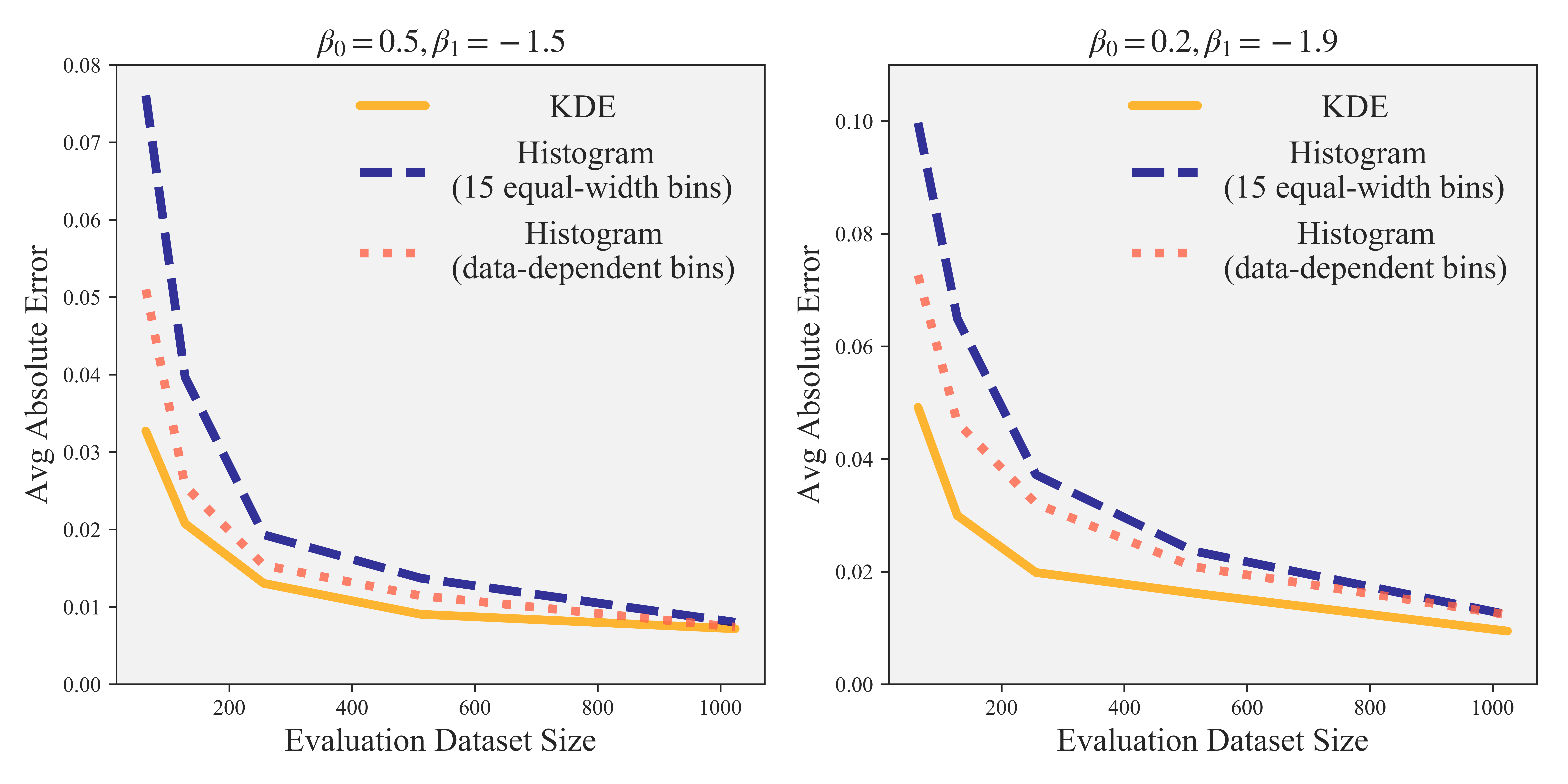
We compare the finite sample performance of proposed KDE-based ECE^d estimator with histogram-based ones on a synthetic binary classification problem  (Vaicenavicius et al., 2019). The classifier is parameterized by two parameters $\beta_{0},\beta_{1}$ (described in detail in supplementary material Sec. E). We consider a less-calibrated case $\beta_{0}=0.5,\beta_{1}=-1.5$, and a better-calibrated case with $\beta_{0}=0.2,\beta_{1}=-1.9$. The canonical calibration probability $\pi^{(f)}(z)$ has a closed-form expression (Eq. (14)), allowing us to obtain the ground truth ECE (Eq. (2)) using Monte Carlo integration with $10^{6}$ samples. We compare the ground truth to the estimation of ECE¹ using KDE and histogram-based estimators – one with $15$ equal-width bins and other with data-dependent binning scheme (Sturges, 1926). In Figure 5, we vary the size of evaluation samples $n_{e}$ from $64$ to $1024$ and plot the mean absolute error (averaged over $1000$ independent experiments) between KDE/Histograms estimates and the ground truth. KDE consistently outperforms histogram-based estimators regardless of the binning schemes. The discrepancy is particularly noticeable with small $n_{e}$, highlighting KDE’s superior efficiency in data-limited regime. In rest of the paper, we adopt KDE for estimating ECE, unless otherwise specified. Additional results can be found in the supplementary material, e.g., the distribution of the estimation errors in Figure 7 and comparison of the proposed KDE estimators with recently proposed debiased histogram ECE estimators (Kumar et al., 2019) in Figure 9.

Figure 5: Average absolute error for different ECE estimators as a function of the number of samples used in the ECE estimation. KDE-based ECE estimator achieves lower estimation error, especially when the evaluation dataset is small.

5.2 Calibrating Neural Network Classifiers

We calibrate various deep neural network classifiers on popular computer vision datasets: CIFAR-10/100 (Krizhevsky, 2009) with 10/100 classes and ImageNet (Deng et al., 2009) with 1000 classes. For CIFAR-10/100, we trained DenseNet (Huang et al., 2017), LeNet (LeCun et al., 1998), ResNet (He et al., 2016) and WideResNet (WRN) (Zagoruyko & Komodakis, 2016). The training detail is described in Sec. F. We use 45000 images for training and hold out 15000 images for calibration and evaluation. For ImageNet, we acquired 4 pretrained models from (Paszke et al., 2019) which were trained with $1.3$ million images, and $50000$ images are hold out for calibration and evaluation.

We compare seven calibration methods: for parametric approaches, we use TS, our proposed three-component model ensemble approach ETS, and the Dirichlet calibration with off-diagonal regularization (DirODIR) (Kull et al., 2019). Following (Kumar et al., 2019), we use the squared error as the loss function to fit TS and ETS. For non-parametric approaches, we compare IROvA, our proposed multi-class accuracy-preserving scheme IRM, and the composition method that combines IROvA with TS as described in Sec. 3.3 (referred to as IROvA-TS). In addition, we include the Gaussian Process calibration (GPC) (Wenger et al., 2020). Among all examined methods, only TS, ETS and IRM are accuracy-preserving.

Figure 6: Learning curve comparisons of various calibration methods on top-label ECE¹ (top) and the classification accuracy (bottom).

For our first experiment, we adopt a standard calibration setup (Guo et al., 2017) with fixed-size calibration $n_{c}$ and evaluation $n_{e}$ datasets. We randomly split the hold-out dataset into $n_{c}=5000$, $n_{e}=10000$ for CIFAR-10/100 and $n_{c}=n_{e}=25000$ for ImageNet. We randomly split the hold-out dataset into $n_{c}$ calibration points to learn the calibration map, and $n_{e}$ evaluation points to evaluate ECE and classification accuracy. All results are averaged over $100$ independent runs. On ImageNet, GPC fails to converge due to its high computational cost, thus we exclude its results.

Table 1 displays top-label ECE¹ and Table 2 displays the calibration gain $\Delta$ECE². Overall the rankings of calibration methods by top-label ECE¹ or by $\Delta$ECE² are very similar. Our proposed strategies consistently lead to better performance than the baseline implementations (ETS over TS; IRM and IROvA-TS over IROvA). Depending on the model/data complexity, either parametric or non-parametric variants may be more suitable.

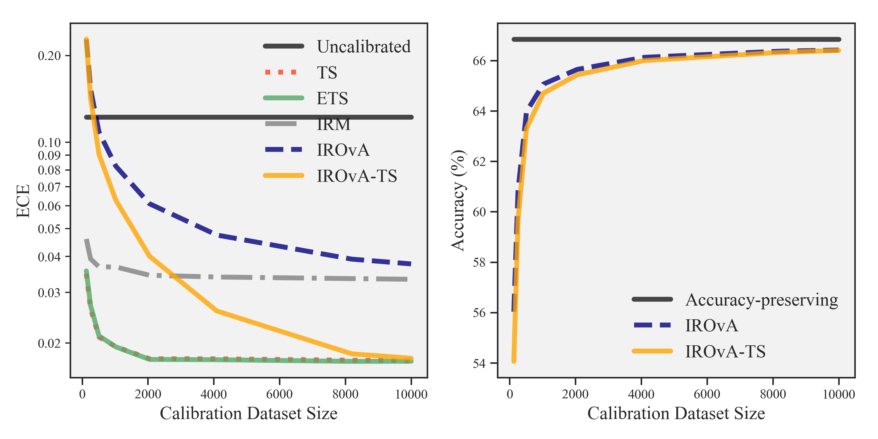
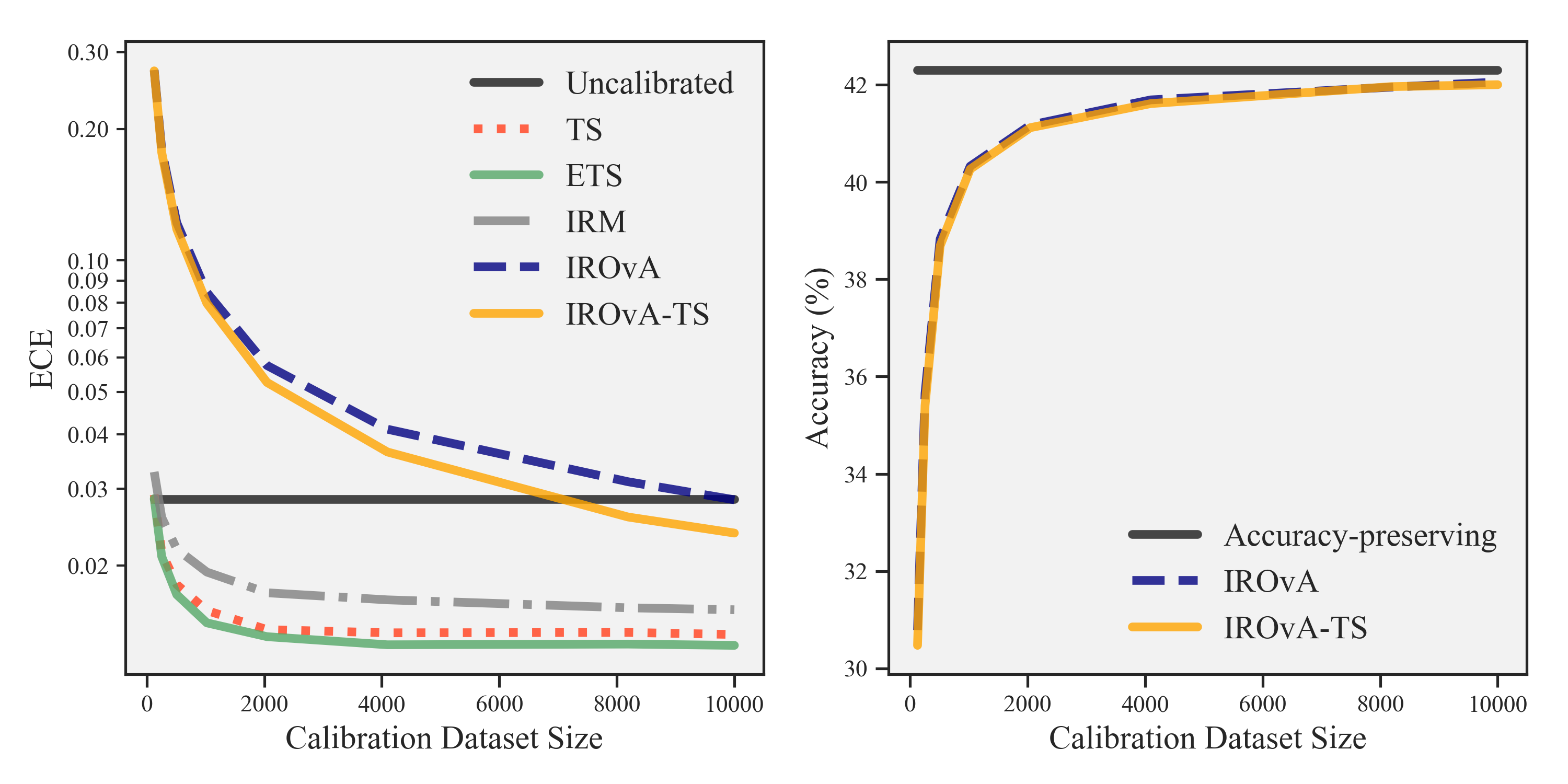
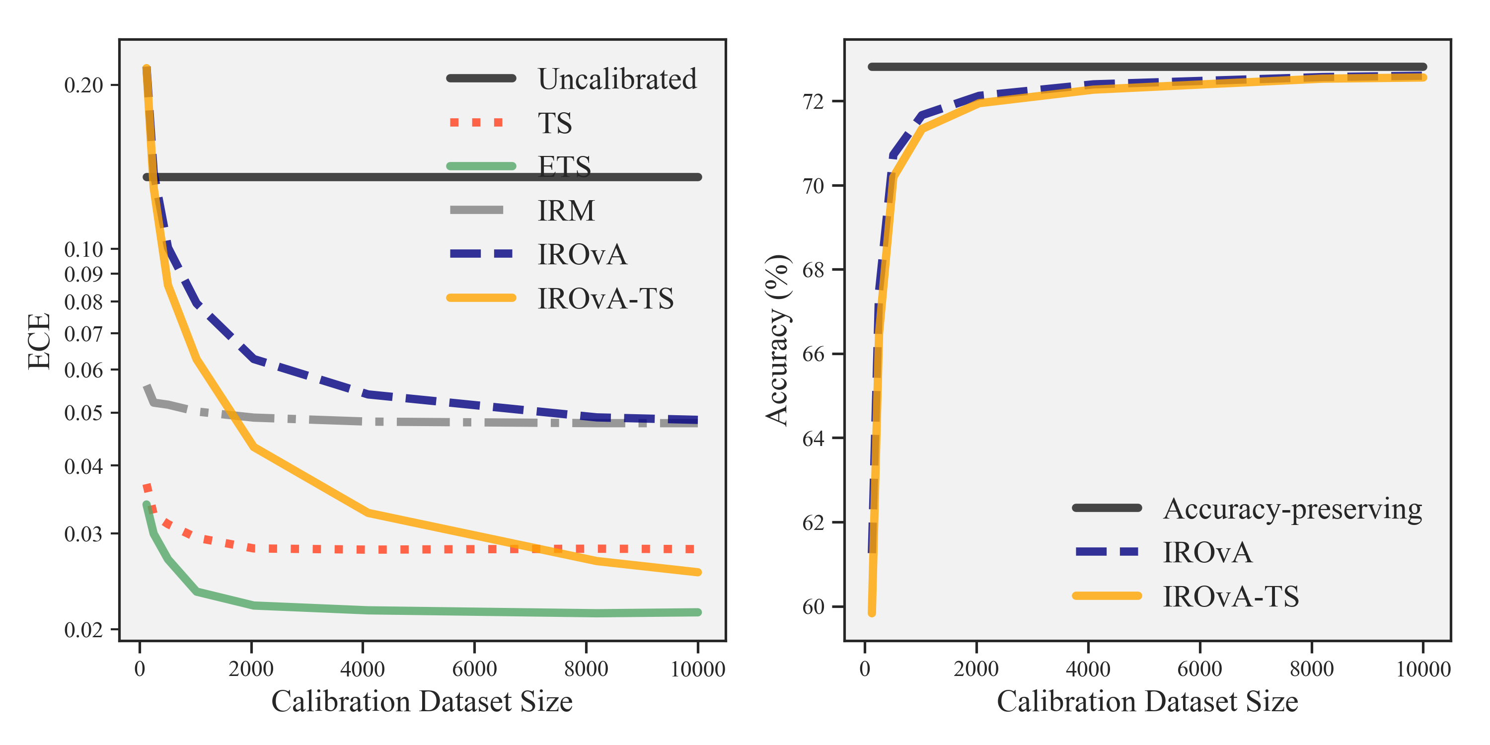
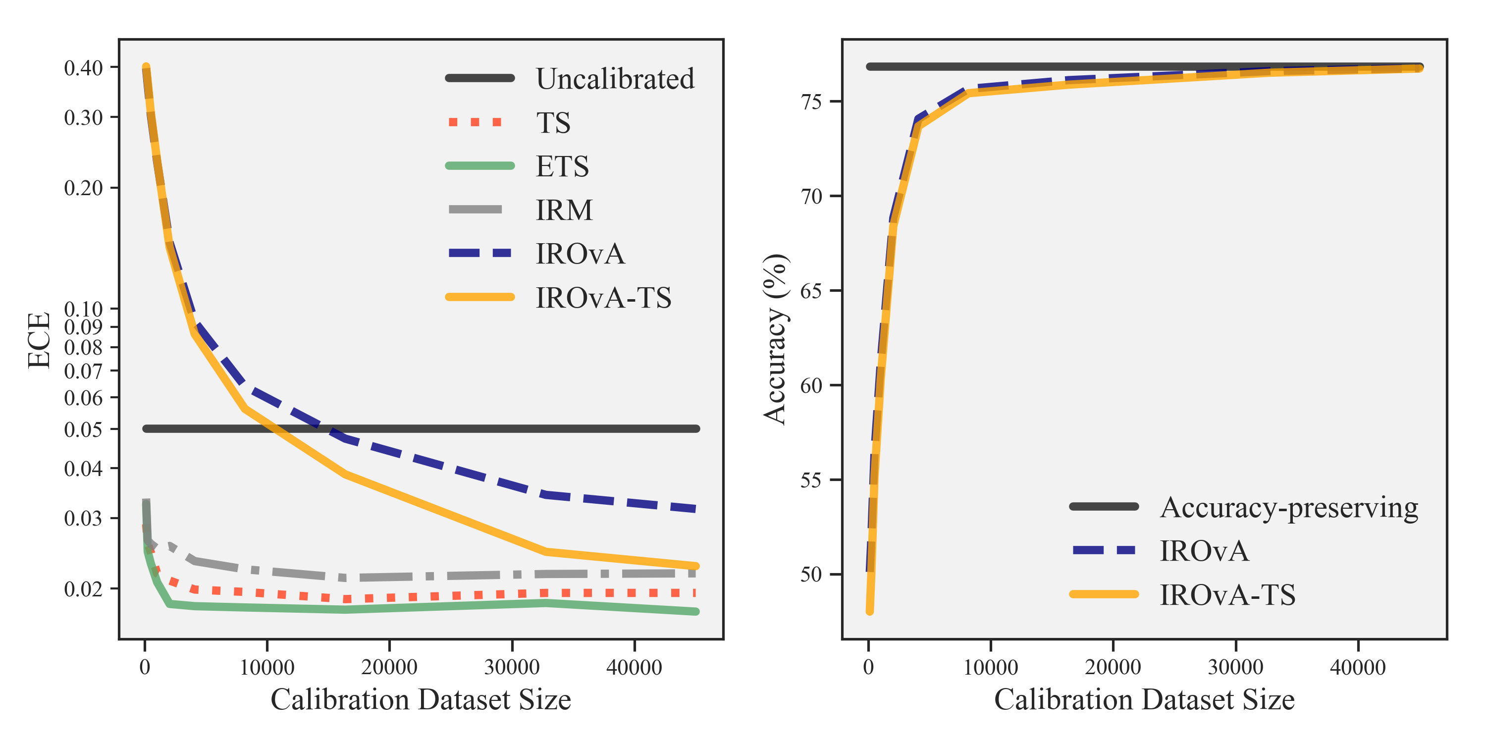
Note that calibration methods may perform differently with varying amounts of calibration data. A critically missing aspect of the standard practice of fixed-size comparison is that it does not reveal the data-amount-dependent behavior, and it may provide an incomplete picture of the calibration method’s performance. To explore this holistically, we next conduct a learning curve analysis by varying the calibration dataset size and evaluating three desiderata-related properties (accuracy, data-efficiency and expressivity) of calibration approaches. While such learning curve analysis has been extensively used in the standard machine learning literature, its use in the calibration of deep neural network classifiers is scarce. Specifically, we reserve the same set of $5000$ data points for evaluation, and vary the number of calibration data from $128$ to $10000$ (CIFAR-10/100) or $45000$ (ImageNet). This process is repeated 100 times on the baseline (TS, IROvA) and their variants (ETS, IRM, IROvA-TS) to validate the effectiveness of Mix-n-Match.

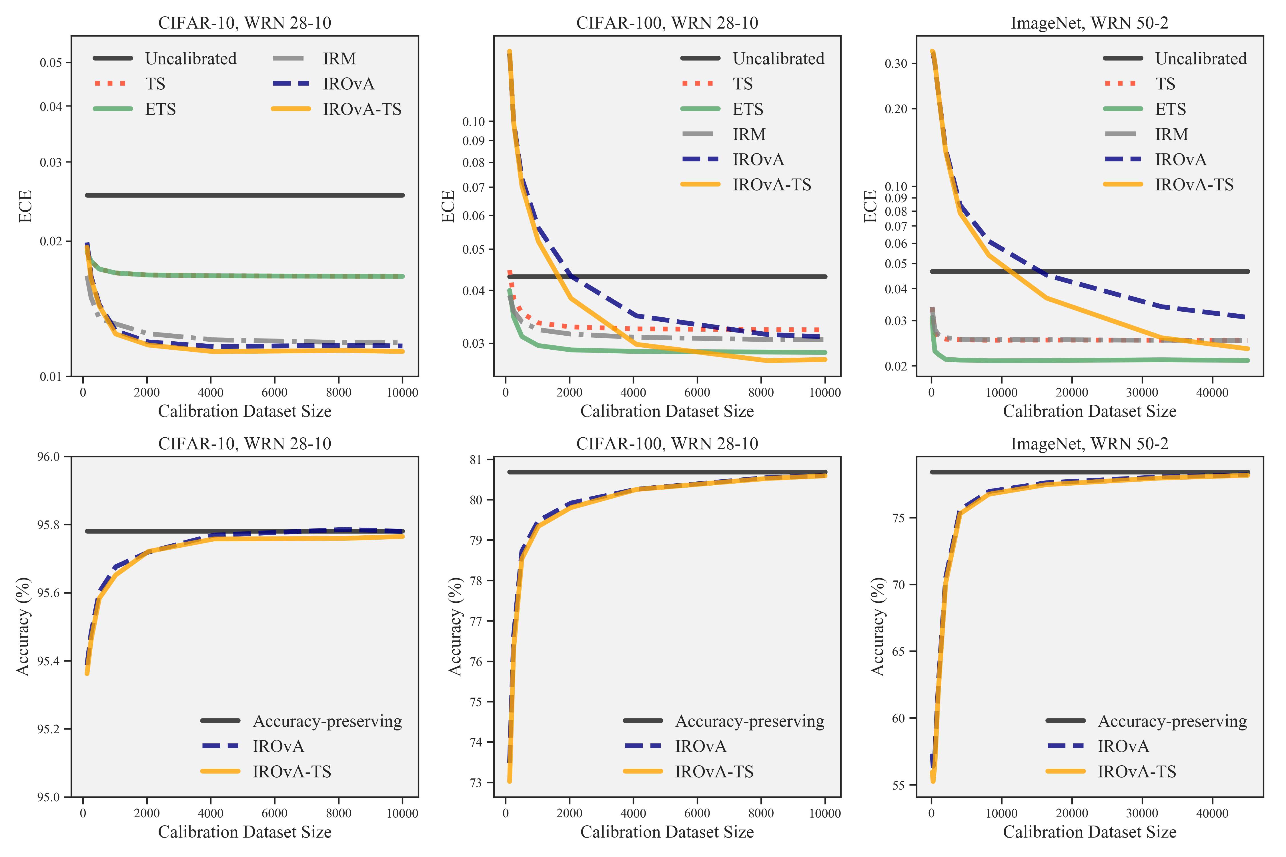
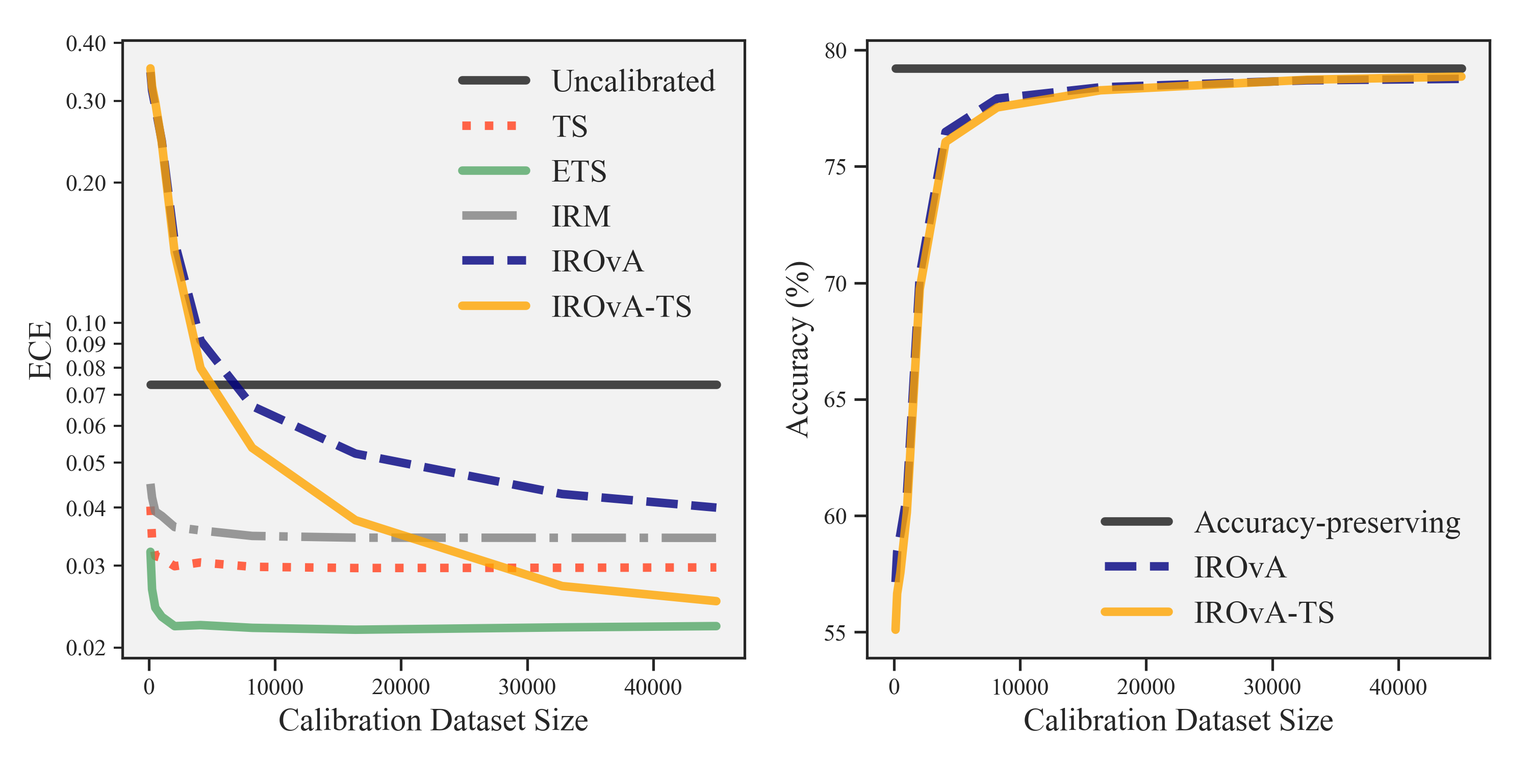
For Wide ResNets, Figure 6 shows how the average ECE and the accuracy over the repetitions change as a function of calibration dataset size $n_{c}$. Results for other cases are provided in the supplementary material Sec. F. We provide a thorough analysis on the learning curves below.

Accuracy. From Figure 6 bottom, we observe that IROvA and IROvA-TS lead to serious accuracy reduction in the data-limited regime, and require a large calibration datasets to recover the original accuracy, while the accuracy-preserving approaches maintain the accuracy.

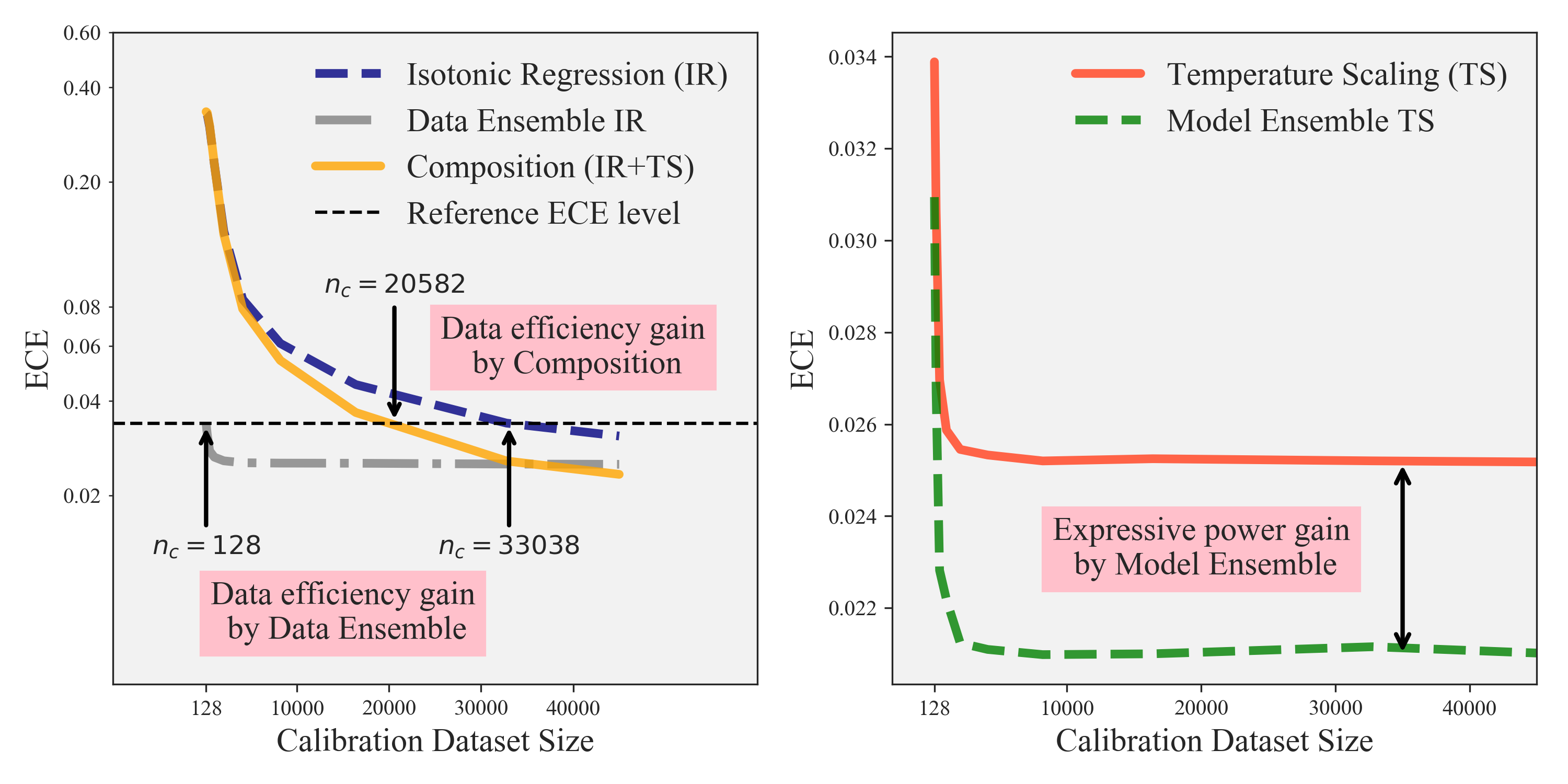
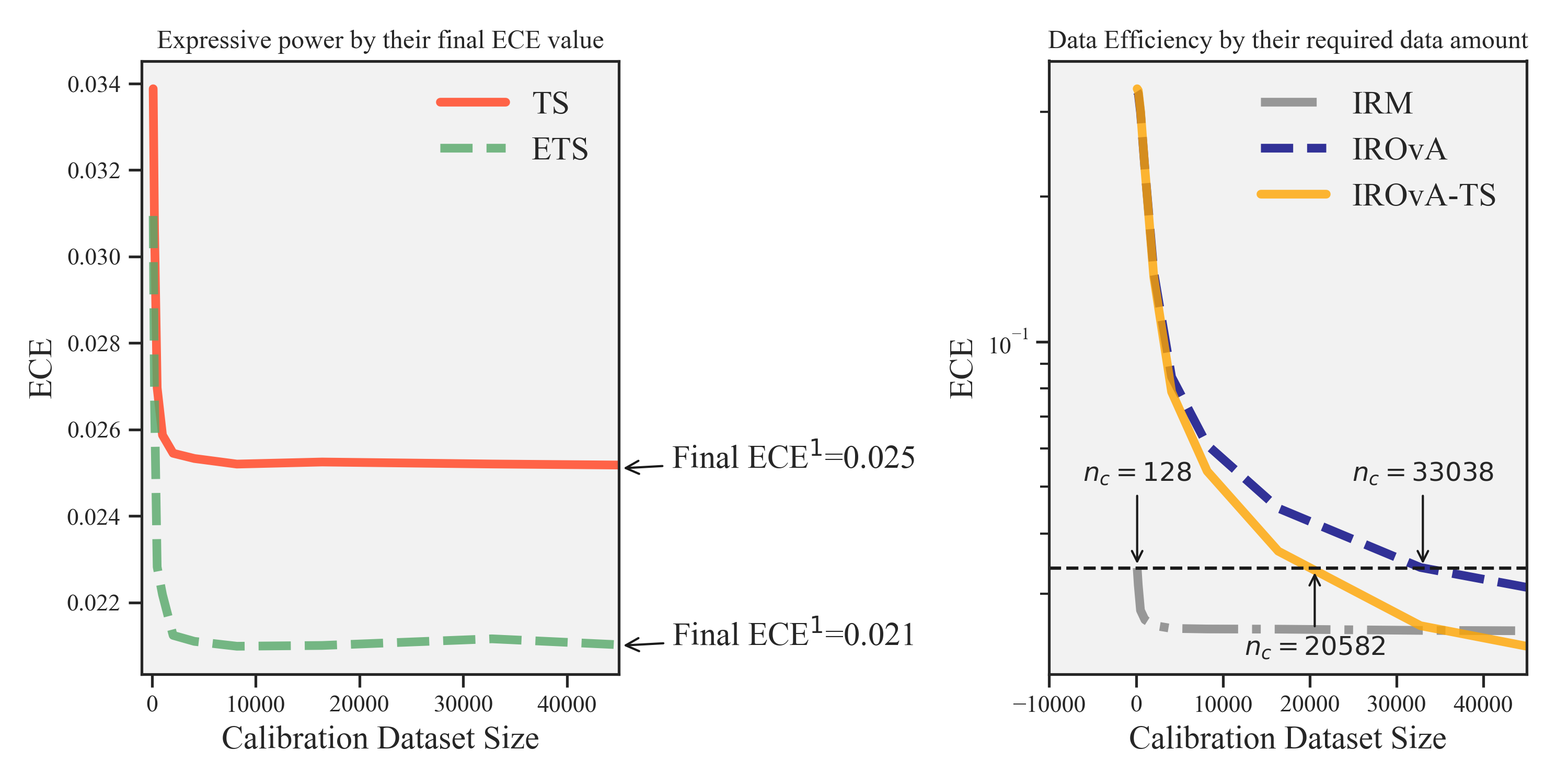
Data-efficiency. Parametric methods (TS, ETS) enjoy the fastest converge of ECE (see Figure 6 top), which is anticipated. Our proposed data ensemble (IRM) and compositional (IROvA-TS) solutions also converge faster than IROvA. To quantify their data-efficiency gain, we record the required amount of data for non-parametric approaches to reach a reference calibration level (see Figure 10 right) in Table 4. The proposed data ensemble and compositional approaches achieve remarkable data-efficiency gains.

Expressivity. Note that a more expressive method should attain lower ECE with a sufficiently large calibration dataset. From Figure 6 top, we see that the proposed ensemble approach ETS is significantly more expressive than TS. This gain is particularly visible in many-class datasets, e.g., CIFAR-100 and ImageNet, where the canonical calibration function is expected to be complex. Also, the reduced expressivity of IRM over IROvA can be observed, verifying our hypothesis of its efficiency-expressivity trade-off. In Table 3, we provide a quantitative comparison on the expressivity of TS and ETS by measuring their final ECE (at the highest values of $n_{c}$, see Figure 10 left). We see that ETS is consistently more expressive and achieves lower final ECE value than TS across different models/datasets.

Finally, we provide general guidelines on choosing an appropriate calibration method. We recommend ETS for general use and IRM as a strong alternative when the parametric form of ETS is misspecified (see Figure 6 left). Both approaches are accuracy-preserving and can be compared based on the proposed calibration gain metric. For complex calibration tasks, we recommend IROvA-TS if a large calibration dataset is available and the user does not have hard constraints on preserving the accuracy (see Figure 6 middle-right). We expand the analysis and the recommendation in the supplementary material Sec. G.

To summarize, our proposed Mix-n-Match strategies provide substantial benefits for calibration, and can be easily incorporated into many existing calibration methods. We also provide guidelines on determining the most appropriate calibration method for a given problem in Sec. G. We expect the observed trends to generalize to other potential extensions. For example, the ensemble beta scaling method should be more expressive than the original beta scaling method (Kull et al., 2017), and the composition of TS with other non-parametric methods, e.g., IRM, should also be more data-efficient. We also anticipate additional efficiency gain if one substitutes TS with ETS in the composition, since ETS has been shown to be more expressive.

6 Conclusion

We demonstrated the practical importance of designing calibration methods with provable accuracy-preserving characteristics, high data-efficiency, and high expressivity. We proposed general Mix-n-Match calibration strategies (i.e., ensemble and composition) to extend existing calibration methods to fulfill such desiderata simultaneously. Furthermore, we proposed a data-efficient kernel density-based estimator for a reliable evaluation of the calibration performance. Comparisons with existing calibration methods across various datasets and neural network models showed that our proposed strategies consistently outperform their conventional counterparts. We hope that our developments will advance research on this essential topic further.

Appendix A Proofs of Proposition 3.1: Accuracy-Preserving Calibration Maps

For an arbitrary pair of classes ($\forall i,j\in[L]$, where $[L]$ denotes the set of positive integers up to $L$) of the prediction probability vector z, let us assume that $z_{i}<z_{j}$ without loss of generality. By definition, the strictly isotonic function $g$ will output $g(z_{i})<g(z_{j})$ after the transformation. After dividing by the same normalization constant $G(z)$, the following relationship holds: $[T(z)]_{i}<[T(z)]_{j}$, where $[.]_{i}$ represents the $i$-th entry of the vector. Since the order of entries in the prediction vector is unchanged after the calibration, the classification accuracy is preserved.

Appendix B Proofs of Theorem 4.1: Statistical Properties of KDE-based ECE

Mirror image KDE for boundary correction. Considering that we work with the probability simplex $\Delta^{L}$ in the context of calibration, KDE can suffer from excessively large bias near the boundary of the simplex. To suitably correct for boundary bias without compromising the estimation quality, we adopt the mirror image KDE strategy (Singh & Póczos, 2014b). The convergence/consistency properties will be proved for such a choice.

Smoothness assumption on the underlying densities. Let $\beta$ and $N$ be positive numbers. Given a vector $s=(s_{1},\ldots,s_{L})$ with non-negative integer entries, let us use $D^{s}:=\frac{\partial^{\lVert s\rVert_{1}}}{\partial^{s_{1}}z_{1}\ldots\partial^{s_{L}}z_{L}}$ to denote the differential operator. The $\beta$-Hölder class of densities $\Sigma(\beta,N)$ contains those densities $p:[0,1]^{L}\rightarrow\mathbb{R}$ satisfying the following relationship:

$$|D^{s}p(z)-D^{s}p(z^{\prime})|\leq N\lVert z-z^{\prime}\rVert^{\beta-\lVert s\rVert_{1}},$$

for all $z,z^{\prime}\in\mathcal{Z}$ and all $s$ with $\lVert s\rVert_{1}=\beta-1$. We assume that the distribution for predictions $p(z)$ as well as the calibration probabilities $\pi_{l}$ for each class $l\in[L]$ belongs to the $\beta$-Hölder class.

Assumption on the kernel function. We assume that the kernel function $K:\mathbb{R}\rightarrow\mathbb{R}_{\geq 0}$ has bounded support $[-1,1]$ and satisfies:

$$\int_{-1}^{1}K(u)\mathop{du}=1;\lVert K\rVert_{1}=\int_{-1}^{1}|K(u)|\mathop{du}<\infty;\forall j\in[\beta-1],\int_{-1}^{1}u^{j}K(u)\mathop{du}=1.$$

Boundedness assumption. We denote $C_{\pi}:=\text{sup}_{z}\lVert z-\pi(z)||_{1}$ and $C_{z}:=\text{sup}_{z}\tilde{p}(z)$ and assume they are both finite.

We can bound the KDE estimation error of $|\text{ECE}(f)-\widetilde{\text{ECE}}(f)|$ after applying the triangle inequality:

$$\begin{split}&|\text{ECE}(f)-\widetilde{\text{ECE}}(f)|=\bigg{|}\int\lVert z-\pi(z)\rVert_{1}p(z)\mathop{dz}-\int\lVert z-\tilde{\pi}(z))\rVert_{1}\tilde{p}(z)\mathop{dz}\bigg{|}\\ &\leq\int\bigg{|}p(z)\lVert z-\pi(z)\rVert_{1}-\tilde{p}(z)\lVert z-\pi(z)\rVert_{1}\bigg{|}\mathop{dz}+\int\bigg{|}\tilde{p}(z)\big{(}\lVert z-\pi(z)\rVert_{1}-\lVert z-\tilde{\pi}(z)\rVert_{1}\big{)}\bigg{|}\mathop{dz}\\ &\leq\text{sup}_{z}\lVert z-\pi(z)\rVert_{1}\int|p(z)-\tilde{p}(z)|\mathop{dz}+\text{sup}_{z}\tilde{p}(z)\int\lVert\pi(z)-\tilde{\pi}(z)\rVert_{1}\mathop{dz}\\ &\leq C_{\pi}\int|p(z)-\tilde{p}(z)|\mathop{dz}+C_{z}\int\lVert\pi(z)-\tilde{\pi}(z)\rVert_{1}\mathop{dz}\end{split}$$ (9)

which connects the absolute estimation error of ECE to the integrated estimation errors on the unknown densities $p(z)$ and $\pi(z)$. We then borrow the established convergence rate and consistency proofs for (conditional) density functional of mirror KDE (Singh & Póczos, 2014a) to derive the statistical properties for the proposed KDE-based ECE estimator.

Bias convergence rate. Taking the expectation and applying the Fubini’s theorem on both sides in Eq. (9), we can derive:

$$\mathbb{E}|\text{ECE}(f)-\widetilde{\text{ECE}}(f)|\leq C_{\pi}\int\mathbb{E}|p(z)-\tilde{p}(z)|\mathop{dz}+C_{z}\int\mathbb{E}\lVert\pi(z)-\tilde{\pi}(z))\rVert_{1}\mathop{dz}$$

$$\leq C_{\pi}C_{B1}(h^{\beta}+h^{2\beta}+\frac{1}{n_{e}h^{L}})+C_{z}C_{B_{2}}(h^{\beta}+h^{2\beta}+\frac{1}{n_{e}h^{L}})\leq C(h^{\beta}+h^{2\beta}+\frac{1}{n_{e}h^{L}}),$$

where $C_{B1}$ and $C_{B2}$ are constants given the sample size $n_{e}$ and bandwidth $h$ and $C=C_{\pi}C_{B1}+C_{z}C_{B2}$. The quantity $h^{2\beta}$ is introduced by the Bias Lemma (Singh & Póczos, 2014b) from the mirror image KDE. For $\int\mathbb{E}|p(z)-\tilde{p}(z)|\mathop{dz}$, we follow the standard KDE results (see Prop 1.1,1.2 and 1.2.3 (Tsybakov, 2008)) while the bound on the other term $\int\mathbb{E}\lVert\pi(z)-\tilde{\pi}(z))\rVert_{1}\mathop{dz}$ follows 6.2 in (Singh & Póczos, 2014a) or (Döring et al., 2016; Györfi et al., 2006).

The optimal bandwidth is $h\asymp n_{e}^{-1/(\beta+L)}$, leading to a convergence rate of $O\big{(}n_{e}^{-\beta/(\beta+L)}\big{)}$.

Consistency. Let $\tilde{p}^{\prime}$ denote the KDE marginal density of $z$ when an existing sample point is replaced by a new sample from the same distribution $p(z)$, and similarly $\tilde{\pi}^{\prime}$ denote the KDE canonical calibration function after replacing a sample. Following (Singh & Póczos, 2014a), we can bound the density discrepancy before/after replacing a single sample by:

$$\int|\tilde{p}(z)-\tilde{p}^{\prime}(z)|\mathop{dz}\leq\frac{C_{V1}}{n_{e}};\int\lVert\tilde{\pi}(z)-\tilde{\pi}^{\prime}(z)\rVert_{1}\mathop{dz}\leq\frac{C_{V2}}{n_{e}},$$ (10)

where $C_{V1}$ and $C_{V2}$ are constants in the class-dimension $L$ and the kernel norm $\lVert K\rVert_{1}$ for exact values. Suppose that we use two sets of $n_{e}$ independent samples to estimate $p$ and $\pi$, respectively. Since $\widetilde{\text{ECE}}(f)$ depends on $2n_{e}$ independent variables, combining Eq. (10) with Eq. (9), we can use McDiarmid’s Inequality (McDiarmid, 1989) to derive that:

$$\mathbb{P}(|\widetilde{\text{ECE}}(f)-\mathbb{E}\widetilde{\text{ECE}}(f)|>\varepsilon) \leq 2\exp\bigg{(}-\frac{2\varepsilon^{2}}{2n_{e}(2C_{V}/n_{e})^{2}}\bigg{)}=2\exp\bigg{(}-\frac{\varepsilon^{2}n_{e}}{4C_{V}^{2}}\bigg{)}.$$

for $C_{V}=\max(C_{V1},C_{V2})$. As $\mathbb{P}(|\widetilde{\text{ECE}}(f)-\mathbb{E}\widetilde{\text{ECE}}(f)|>\varepsilon)$ approaches 0 when $n_{e}\rightarrow\infty$, the KDE-based ECE estimator is consistent.

Appendix C KDE Implementation Detail

Kernel function choice. Different types of kernel functions $K(u)$ can be used, such as the Gaussian and Epanechnikov functions. Our choice is the Triweight Kernel $K_{h}(u)=(1/h)\frac{35}{32}(1-(u/h)^{2})^{3}$ on $[-1,1]$, since it has been recommended for problems with limited support interval (de Haan, 1999).

Bandwidth selection. We use the popular rule-of-thumb $h=1.06\hat{\sigma}n_{e}^{-1/5}$ (Scott, 1992), where $\hat{\sigma}$ is the standard deviation of the samples.

Appendix D Proof for Proposition 4.2: Calibration Gain for Accuracy-Preserving Methods

According to the calibration refinement decomposition (Murphy, 1973), the expected calibration error ECE² is equal to:

$$\text{ECE}^{2}(f)=\mathbb{E}\lVert z-\pi(z)\rVert_{2}^{2}=\mathbb{E}\lVert z-y\rVert_{2}^{2}-\mathbb{E}\lVert\pi(z)-y\rVert_{2}^{2},$$ (11)

where $\mathbb{E}\lVert z-y\rVert_{2}^{2}$ is the standard square loss and $\mathbb{E}\lVert\pi(z)-y\rVert_{2}^{2}$ is the refinement error (Murphy, 1973) that penalizes the existence of inputs sharing the same prediction but different class labels. Before proceeding further, we first introduce the definition of injective calibration maps:

Definition D.1 (Injective Calibration Map).

The calibration map is injective if different prediction vectors remain different after calibration: $\forall z,z^{\prime}\in\mathcal{Z},T(z)\neq T(z)\text{ if }z\neq z^{\prime}$.

Proposition D.1.

The accuracy-preserving calibration map $T$ in Def. 3.1is injective.

Proof.

Given $z\neq z^{\prime}$, without loss of generality assume $G(z)\geq G(z^{\prime})$ for their normalization constants. Since $z\neq z^{\prime}$, there must exists at least one class $l$ where $z_{l}<z_{l}^{\prime}$. After the transformation by a strictly isotonic function $g$, we know that $g(z_{l})<g(z^{\prime}_{l})$. Then we can derive that:

$$[T(z)]_{l}-[T(z^{\prime})]_{l}=\frac{g(z_{l})}{G(z)}-\frac{g(z_{l}^{\prime})}{G(z^{\prime})}=\frac{g(z_{l})G(z^{\prime})-g(z_{l}^{\prime})G(z)}{G(z)G(z^{\prime})}<0.$$

Therefore, $T(z)\neq T(z^{\prime})$ because their $l$-th entry is not equal. The calibration map is then injective.

Note that the canonical calibration function in Eq. (1) is essentially the conditional expectation of binary random variables $Y$, as $\pi_{l}(z)=\mathbb{P}[Y_{l}=1|f(X)=z]=\mathbb{E}[Y_{l}|f(X)=z]$. By elementary properties of the conditional expectation, one can easily show that injective calibration maps will not change the canonical calibration probabilities, thus $\pi(z)=\pi(T(z))$ for injective $T$. Combining this with the decomposition relationship in Eq. (11), we can show that:

$$\begin{split}\Delta\text{ECE}^{2}(T)&=\text{ECE}^{2}(f)-\text{ECE}^{2}(T\circ f)\\ &=\mathbb{E}\lVert z-y\rVert_{2}^{2}-\mathbb{E}\lVert\pi(z)-y\rVert_{2}^{2}-\big{(}\mathbb{E}\lVert T(z)-y\rVert_{2}^{2}-\mathbb{E}\lVert\pi(T(z))-y\rVert_{2}^{2}\big{)}\\ &=\mathbb{E}\lVert z-y\rVert_{2}^{2}-\mathbb{E}\lVert T(z)-y\rVert_{2}^{2}.\end{split}$$ (12)

Therefore, after applying an injective calibration map, which include the proposed accuracy-preserving ones, any changes in the squared loss will be due to the change in ECE². ∎

Remark. Most existing calibration methods are not injective. For example, in histogram binning (Zadrozny & Elkan, 2001) or the original isotonic regression method (Zadrozny & Elkan, 2002), all predictions inside certain intervals will be mapped to be identical, and violate the injective requirement. For parametric methods, such as vector, matrix (Guo et al., 2017), or Dirichlet scaling (Kull et al., 2019), different logits can be transformed to produce the same prediction probability vectors, and violate the injective requirement.

Appendix E Experimental Details and Additional Results in Section 5.1

E.1 Experimental details

For the synthetic example, the labels ($Y$) and input features ($X$) are distributed as:

$$\begin{split}\mathbb{P}(Y_{1}=1)=\mathbb{P}(Y_{2}=1)=1/2;\mathbb{P}(X=x|Y_{1}=1)=\mathcal{N}(x;-1,1);\mathbb{P}(X=x|Y_{2}=1)=\mathcal{N}(x;1,1).\end{split}$$ (13)

The probability of observing the label $Y_{1}=1$ conditioned on the input $x$ can be written as:

$$\mathbb{P}(Y_{1}=1|X=x)=1/[1+\exp(2x)].$$

We assume the prediction models to be in the following form, parameterized by $\beta_{0}$ and $\beta_{1}$:

$$z=f(x)=(z_{1},z_{2})=\bigg{(}\frac{1}{1+\exp(-\beta_{0}-\beta_{1}x)},\frac{\exp(-\beta_{0}-\beta_{1}x)}{1+\exp(-\beta_{0}-\beta_{1}x)}\bigg{)}.$$

This leads to close-form expressions for the canonical calibration functions $\pi(z)=(\pi_{1}(z),\pi_{2}(z))$:

$$\pi_{1}(z)=[1+\exp(-2\frac{\beta_{0}+\log(1/z_{1}-1)}{\beta_{1}})]^{-1},\pi_{2}(z))=1-\pi_{1}(z).$$ (14)

Finally, we estimate the ground-truth ECE^d based on Monte Carlo integration: (i) generate $10^{6}$ random input-output sample pairs according to Eq. (13), and (ii) record the sample average value of the quantity $|z_{1}-\pi_{1}(z)|^{d}$ as the ground-truth.

E.2 Additional results

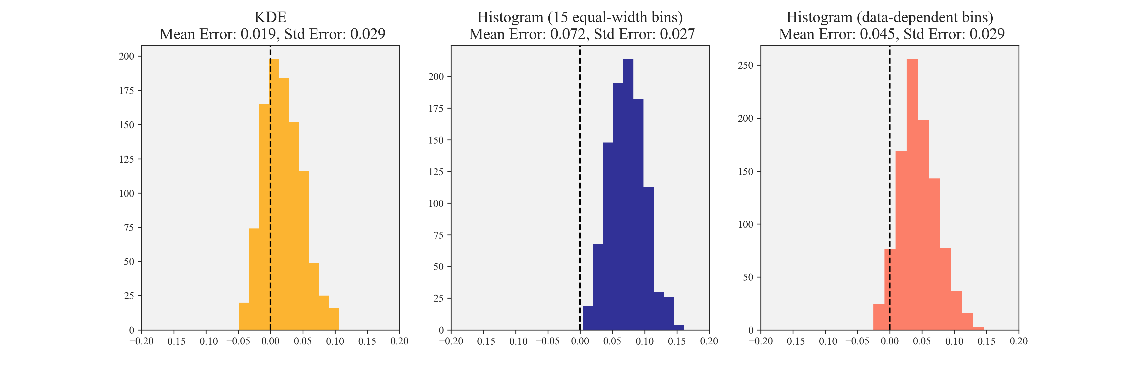
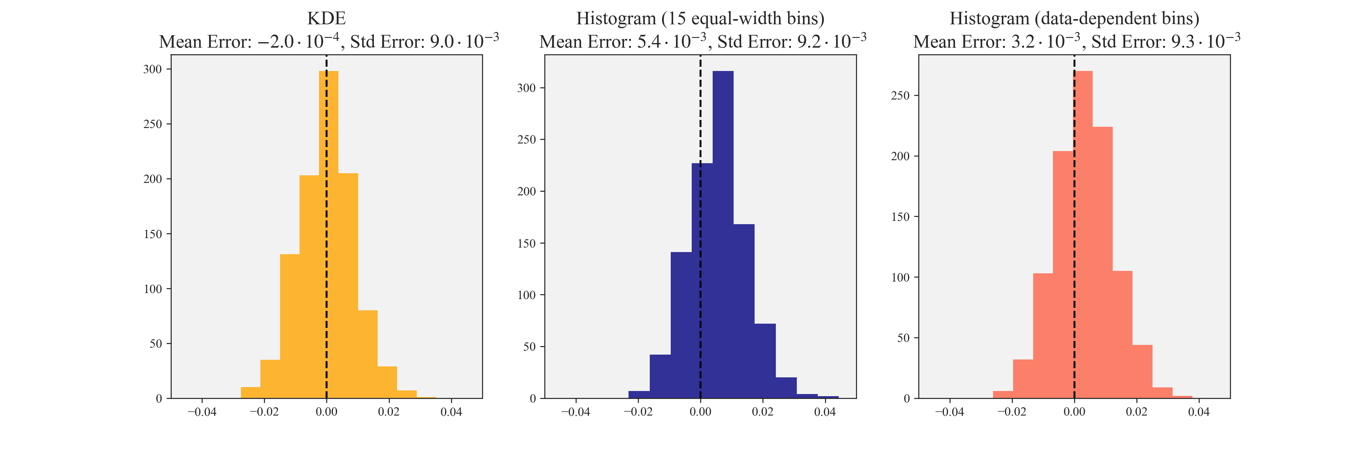
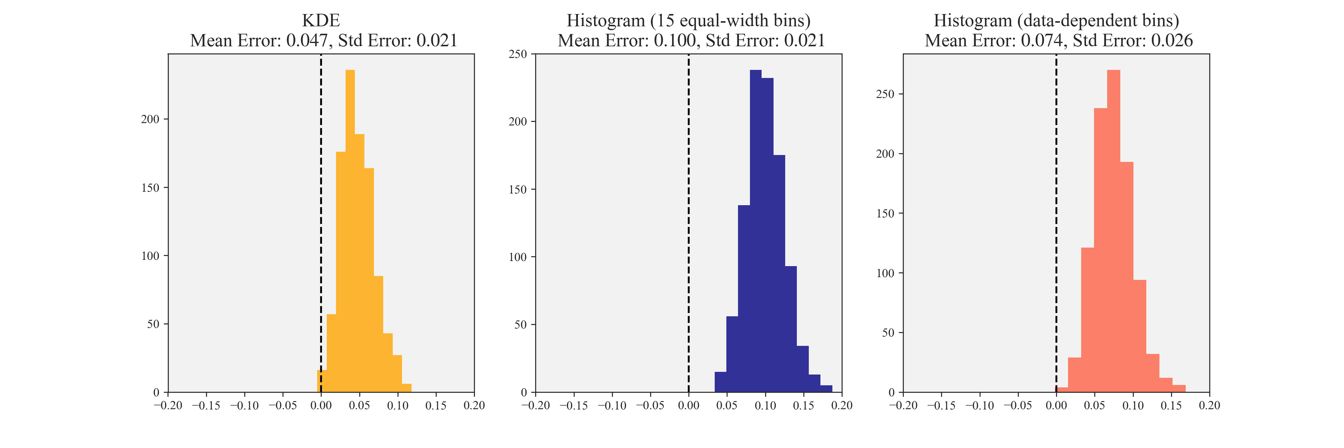
We plot the distribution of the errors between the ECE estimates and the ground-truth ECE in two representative scenarios: a data-limited scenario with $n_{e}=64$ in Figure 7 and a data-rich scenario with $n_{e}=1024$ in Figure 8. The KDE estimation errors are generally less biased (more concentrated around zero) as compared to histograms, corroborating the findings in Sec. 5.1. Judging from the variance of the estimation errors, the KDE estimation errors are generally less dispersed than the two histogram estimators, indicating that the KDE estimators are more reliable. In contrast, histogram ECE estimators tend to severely over-estimates ECE in data-limited regime, with the majority of their estimation errors being positive. Their sensitivity to the binning schemes can be also observed from the distribution discrepancies between using equal-width and data-dependent bins: the histogram estimator with data-dependent bins generally performs better than the one with equal-width bins, although it cannot reach the accuracy level of KDE estimators. However, it performs the worst in the data-rich scenario of Case 2 (Figure 8 bottom).

(a) $n_{e}=64$

(b) $n_{e}=1024$

Figure 7: Distribution of ECE estimation errors in Case 1: $\beta_{0}=0.5,\beta_{1}=-1.5$ with (a) $n_{e}=64$ and, (b) $n_{e}=1024$.

(a) $n_{e}=64$

(b) $n_{e}=1024$

Figure 8: Distribution of ECE estimation errors in Case 2: $\beta_{0}=0.2,\beta_{1}=-1.9$ with (a) $n_{e}=64$, and (b) $n_{e}=1024$.

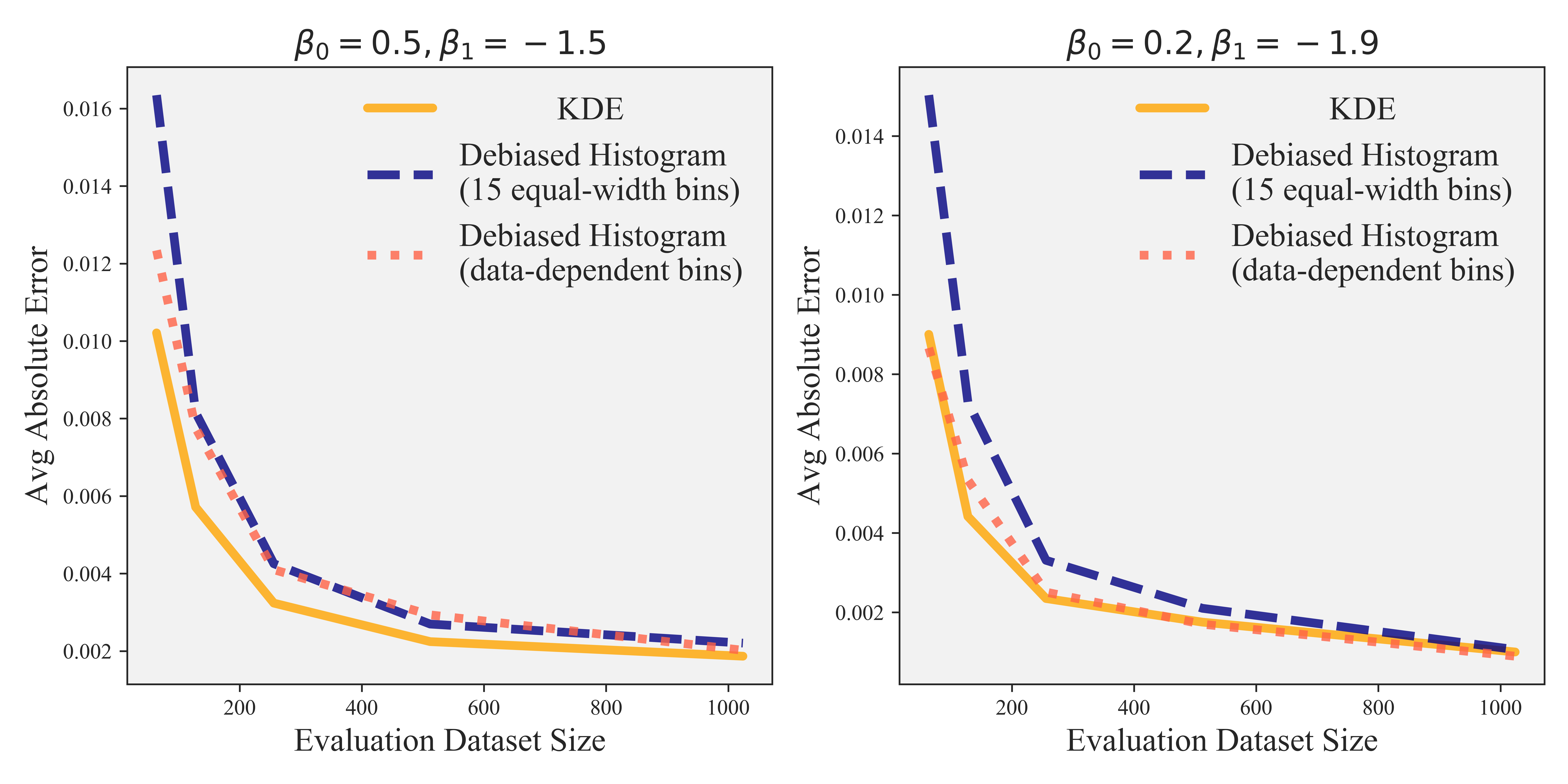
Recently (Kumar et al., 2019) proposed a debiased histogram-based estimator for ECE^d=2, by leveraging error cancellations across different bins. We compare the proposed KDE ECE estimator with the debiased versions of histogram-based ECE estimators with both equal-width and data-dependent binning schemes. We vary the size of evaluation samples $n_{e}$ from $64$ to $1024$ and plot the mean absolute error (averaged over $1000$ independent experiments) between KDE/Debiased-Histograms estimates for ECE² and the ground truth in Figure 9. We observe that KDE-based estimator consistently performs better than the best-performing debiased histogram-based ECE estimators. This agrees with the findings in Sec. 5.1 and confirms the advantage of using KDE-based estimator over histograms-based estimators.

Figure 9: Average absolute error for KDE ECE and debiased histogram ECE estimators as a function of the number of samples used in the ECE estimation. KDE-based ECE estimator achieves lower estimation error, especially when the evaluation dataset is small.

Appendix F Experimental Detail and Additional Results in Section 5.2

F.1 Training details

For training neural networks on CIFAR-10/100, we use SGD with Nesterov momentum and the cross-entropy loss. The weight decay is set to 0.0005, dampening to 0, momentum to 0.9, and minibatch size to 128. The initial learning rate is set to 0.1, and is dropped by a factor of 0.2 at 60, 120 and 160 epochs. For Wide ResNets, we use a dropout rate of 0.3. We train the models for a total of 500 epochs. We use standard mean/std normalization with flipping and data cropping augmentation as described in (Zagoruyko & Komodakis, 2016) on CIFAR-10/100 images.

F.2 Expanded results

The quantitative measure of expressive power and data-efficiency is illustrated graphically in Figure 10 and discussed in Table 3 and Table 4. To summarize, ETS is comparably expressive to TS on CIFAR-10 and noticeably more expressive on CIFAR-100 and ImageNet. Both IRM and IROvA-TS are more efficient than IROvA. The relative efficiency gain of IRM increases as the problems become more complex. On the other hand, the relative efficiency gain of IROvA-TS appears to be quite stable on a wide range of problems.

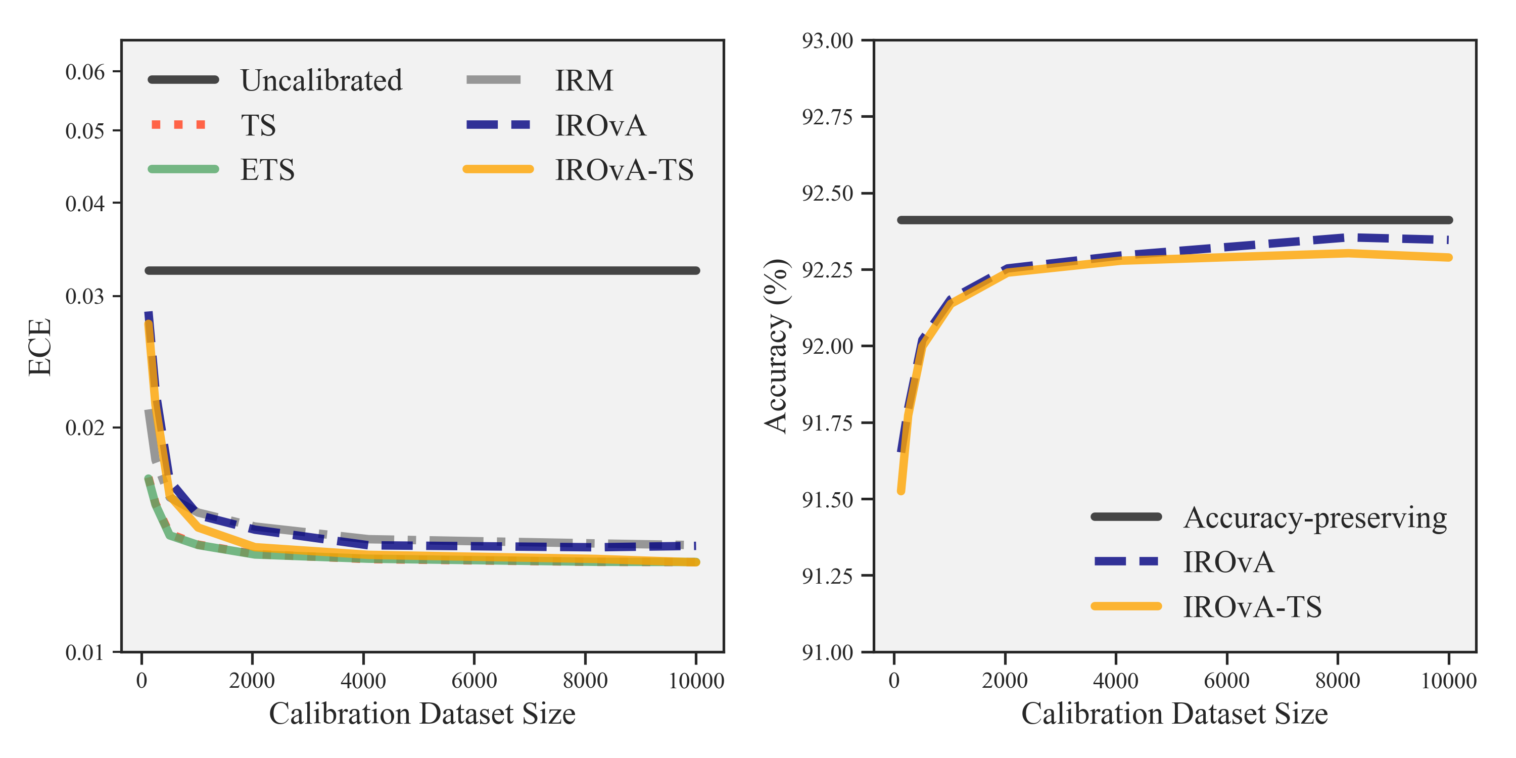
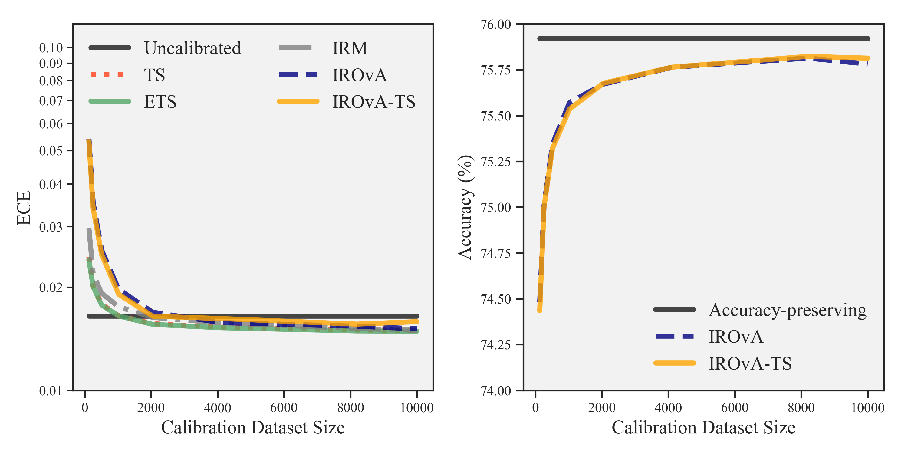
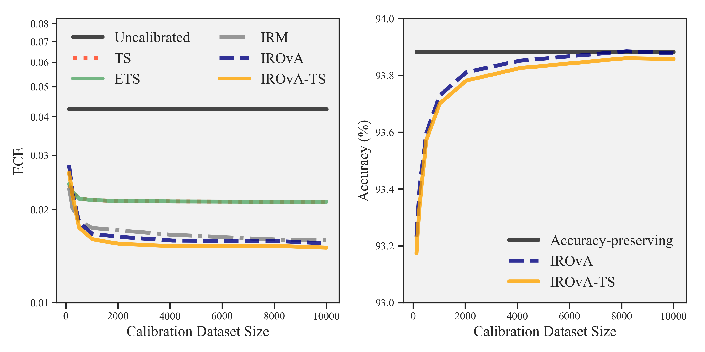
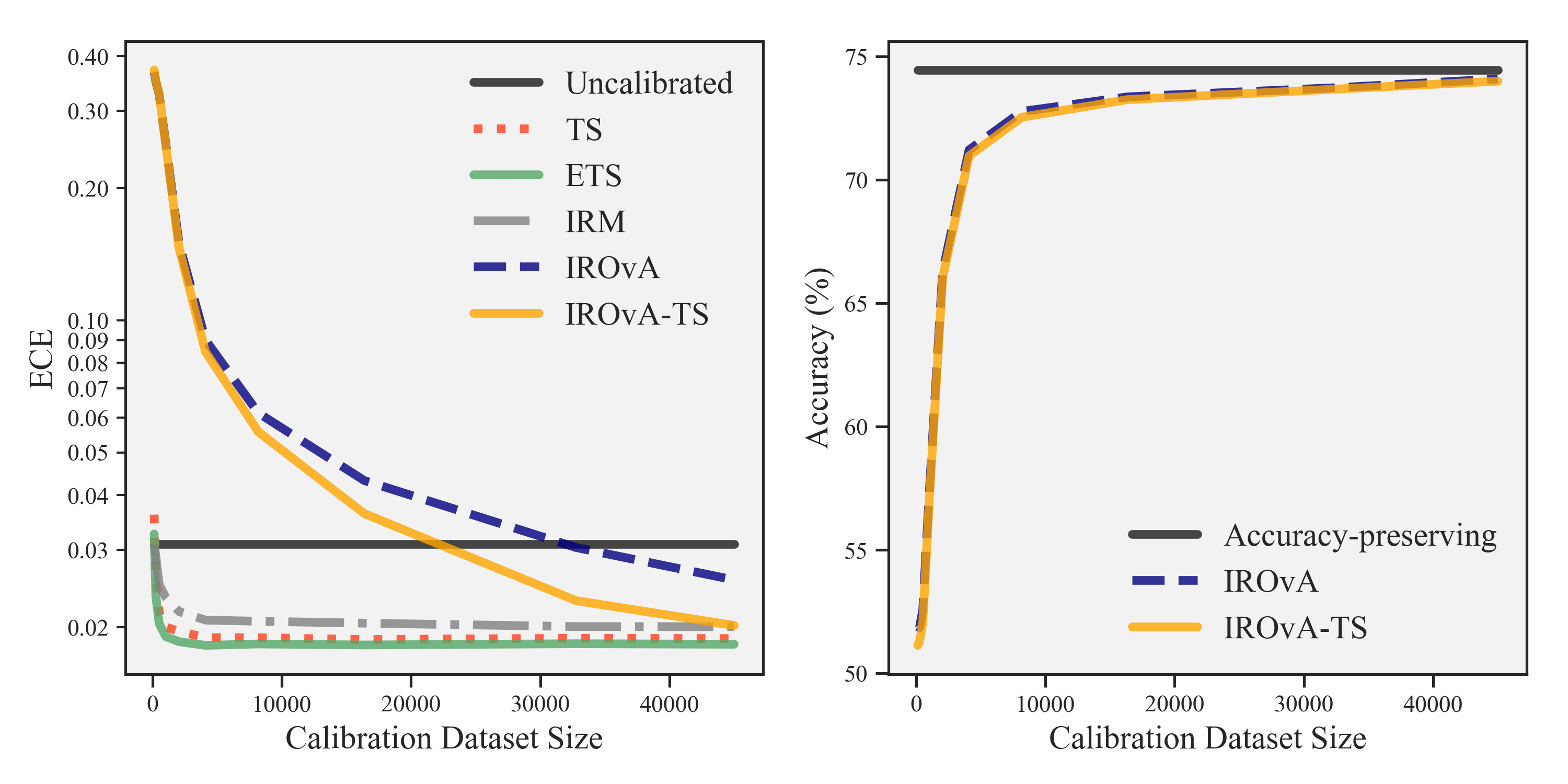
We also provide expanded results on the learning curve analysis for additional neural network classifiers (see Figure 11 to Figure 13). From the visual comparison of the ECE learning curves of ETS and TS, or IRM/IROvA-TS and IROvA, we can confirm the importance to preserve the classification accuracy and the consistent benefit of employing the proposed Mix-n-Match strategies. Overall, in data-limited regime, parametric variants (TS, ETS) perform better than traditional non-parametric variants (IROvA, IROvA-TS) due to their high data-efficiency. ETS significantly outperforms TS and performs the best as the added expressive power from ensembles allow ETS to make further descent on ECE. The proposed accuracy-preserving non-parametric variant IRM also performs good: it is sometimes more effective than TS, although it cannot outperform ETS in most examined cases. The relatively good performance of IRM can be accredited to its high data-efficiency on complex calibration tasks. Going to the data-rich regime, the ECE reduction progress stalls for parametric methods. On complex problems, such as CIFAR-100 and ImageNet, this also applies to the accuracy-preserving non-parametric variants (IRM) due to its expressivity-efficiency trade-off. In contrast, the high expressive power of non-parametric variants (IROvA, IROvA-TS) allow them to keep minimizing the ECE and eventually outperform less expressive methods (ETS, TS or IRM) with sufficient amount of data – although, this cannot be verified in all the examined cases due to our limited data budget. In such regime, the composition method IROvA-TS significantly outperforms IROvA and performs the best due to its enhanced data-efficiency. Based on such observations, our further discussion on the guidelines of calibration methods will be restricted to ETS, IRM and IROvA-TS.

Figure 10: Graphical illustration for the proposed measure of expressive power and data-efficiency.

Table 3: ECE¹ (%) with $n_{c}=10000$ for CIFAR and $n_{c}=45000$ for ImageNet; lower values imply more expressive power.

Dataset	Model	TS	ETS
CIFAR-10	DenseNet 40	1.32	1.32
CIFAR-10	LeNet 5	1.49	1.48
CIFAR-10	ResNet 110	2.12	2.12
CIFAR-10	WRN 28-10	1.67	1.67
CIFAR-100	DenseNet 40	1.73	1.72
CIFAR-100	LeNet 5	1.39	1.31
CIFAR-100	ResNet 110	2.81	2.15
CIFAR-100	WRN 28-10	3.23	2.85
ImageNet	DenseNet 161	1.95	1.75
ImageNet	ResNeXt 101	2.97	2.22
ImageNet	VGG 19	1.89	1.83
ImageNet	WRN 50-2	2.52	2.10

Table 4: Required calibration data amount $n_{c}$ to reach IRM’s performance with $n_{c}=128$ samples; lower value means more data-efficient. All values are normalized (divided by 128) to show how many samples are equivalent to one sample in IRM for each method.

Dataset	Model	IRM	IROvA	IROvA-TS
CIFAR-10	DenseNet 40	1.0	2.45	2.10
CIFAR-10	LeNet 5	1.0	3.15	2.92
CIFAR-10	ResNet 110	1.0	1.84	1.70
CIFAR-10	WRN 28-10	1.0	1.98	1.90
CIFAR-100	DenseNet 40	1.0	37.6	17.9
CIFAR-100	LeNet 5	1.0	58.7	43.0
CIFAR-100	ResNet 110	1.0	28.1	10.7
CIFAR-100	WRN 28-10	1.0	24.2	15.6
ImageNet	DenseNet 161	1.0	282	174
ImageNet	ResNeXt 101	1.0	226	98.6
ImageNet	VGG 19	1.0	251	180
ImageNet	WRN 50-2	1.0	258	161

(a) CIFAR-10+DenseNet 40

(b) CIFAR-10+LeNet 5

(c) CIFAR-10+ResNet 110

Figure 11: Learning curve comparisons of various calibration methods on top-label ECE¹ (left) and the classification accuracy (right) on CIFAR-10 dataset with (a) DenseNet 40 model; (b) LeNet 5 model; and (c) ResNet 110 model.

(a) CIFAR-100+DenseNet 40

(b) CIFAR-100+LeNet 5

(c) CIFAR-100+ResNet 110

Figure 12: Learning curve comparisons of various calibration methods on top-label ECE¹ (left) and the classification accuracy (right) on CIFAR-100 dataset with (a) DenseNet 40 model; (b) LeNet 5 model; and (c) ResNet 110 model.

(a) ImageNet+DenseNet 161

(b) ImageNet+ResNext 101

(c) ImageNet+VGG19

Figure 13: Learning curve comparisons of various calibration methods on top-label ECE¹ (left) and the classification accuracy (right) on ImageNet dataset with (a) DenseNet 161 model; (b) ResNext 101 model; and (c) VGG 19 model.

Appendix G Guidelines

First, we provide guidelines on choosing an appropriate calibration evaluation metric. If knowing the exact value of ECE is important, we recommend KDE-based top-label ECE estimator for its superior data-efficiency as compared to histograms. If the goal is to infer just the rankings not actual calibration errors, one should use the calibration gain metric. It provides a reliable and faithful comparison of different methods based on their actual calibration capabilities. We also note that calibration gain metric might be a lower bound for certain calibration methods, e.g., non accuracy-preserving methods.

We next provide general guidelines on selecting the best calibration method (ETS vs. IRM vs. IROvA-TS), based on: (a) the complexity of the calibration task which is a function of the model complexity (number of free parameters) and the data complexity (number of classes), and (b) resources at hand (the amount of the calibration data).

The complexity of the calibration task is directly related to the complexity of the canonical calibration function in Eq. (1). Although, we do not have the knowledge of the canonical calibration function, we expect a learning task with low model complexity and low data complexity to result in a low complexity calibration task ( see Figure 11 (b)). Next, a learning task with low model complexity but high data complexity (Figure 12 (b)), or high model complexity but low data complexity (Figure 11 (a) and (c)) is expected to result in a moderately complex calibration task. Finally, we expect a learning task with high model & data complexity to result in a highly complex calibration task (Figure 12 (a) and (c), Figure 13).

For low complexity calibration tasks, we see that the performance of uncalibrated models are already satisfactory. This observation agrees with results in (Guo et al., 2017). Further, all the calibration methods perform similarly, however, proposed variants performing slightly better than the baseline approaches. The use case of the most practical interest is where the calibration task is expected to be complex. In such scenarios, an ideal calibration map should have enough expressive power to accurately approximate the canonical calibration function in Eq. (1). However, to fit an expressive calibration map, sufficiently large amount of calibration data is required which may or may not be available. In data limited regime, ETS is recommended as the first choice, while IRM is a potential alternative when the parametric assumptions of ETS are improper (see Figure 6 top left and Figure 11 (c)). In data rich regime, we recommend using IROvA-TS for its high expressive power. For moderate complexity calibration tasks, the patterns are similar to high complexity calibration tasks. The only difference is that the gain of the proposed Mix-n-Match strategies are not as drastic as of the case where calibration task is of high complexity. Of course, if the user has hard-constraints on accuracy-preservation, the choice would be limited to the accuracy-preserving calibrators regardless of the data size or the task complexity. In such scenarios, we recommend ETS and IRM. We also want to emphasize that both ETS and IRM are fairly efficient and perform well on all ranges of the calibration data size.

In summary, our take-home messages on the most appropriate calibration method are the following:

• For complex calibration task (poorly calibrated model, large number of classes), when a large calibration dataset is available and the user does not have hard constraints on preserving accuracy, the proposed compositional method IROvA-TS is recommended to achieve the best degree of calibration.

• For all other cases, the proposed ensemble method ETS is recommended when the parametric assumption is proper. IRM is a strong alternative to be considered in order to avoid the risk of parametric form mis-specification of ETS in certain cases. Both approaches preserve the classification accuracy, and one can conveniently compare them based on the proposed calibration gain metric.

References

- Ashukha et al. (2020) Ashukha, A., Lyzhov, A., Molchanov, D., and Vetrov, D. Pitfalls of in-domain uncertainty estimation and ensembling in deep learning. In International Conference on Learning Representations (ICLR), 2020.
- Ayer et al. (1955) Ayer, M., Brunk, H. D., Ewing, G. M., Reid, W. T., and Silverman, E. An empirical distribution function for sampling with incomplete information. The Annals of Mathematical Statistics, pp. 641–647, 1955.
- Blundell et al. (2015) Blundell, C., Cornebise, J., Kavukcuoglu, K., and Wierstra, D. Weight uncertainty in neural networks. In International Conference on Machine Learning (ICML), pp. 1613–1622, 2015.
- Bröcker (2009) Bröcker, J. Reliability, sufficiency, and the decomposition of proper scores. Quarterly Journal of the Royal Meteorological Society, 135(643):1512–1519, 2009.
- Buja et al. (2005) Buja, A., Stuetzle, W., and Shen, Y. Loss functions for binary class probability estimation and classification: Structure and applications. Technical report, University of Pennsylvania, 2005.
- Chen et al. (2015) Chen, C., Seff, A., Kornhauser, A., and Xiao, J. Deepdriving: Learning affordance for direct perception in autonomous driving. In Proceedings of the IEEE International Conference on Computer Vision (ICCV), pp. 2722–2730, 2015.
- Dawid (1982) Dawid, A. P. The well-calibrated bayesian. Journal of the American Statistical Association, 77(379):605–610, 1982.
- de Haan (1999) de Haan, P. On the use of density kernels for concentration estimations within particle and puff dispersion models. Atmospheric Environment, 33(13):2007–2021, 1999.
- Deng et al. (2009) Deng, J., Dong, W., Socher, R., Li, L.-J., Li, K., and Fei-Fei, L. Imagenet: A large-scale hierarchical image database. In Proceedings of the IEEE Conference on Computer Vision and Pattern Recognition (CVPR), pp. 248–255, 2009.
- Ding et al. (2020) Ding, Y., Liu, J., Xiong, J., and Shi, Y. Revisiting the evaluation of uncertainty estimation and its application to explore model complexity-uncertainty trade-off. In Proceedings of the IEEE/CVF Conference on Computer Vision and Pattern Recognition Workshops, pp. 4–5, 2020.
- Döring et al. (2016) Döring, M., Györfi, L., and Walk, H. Exact rate of convergence of kernel-based classification rule. In Challenges in Computational Statistics and Data Mining, pp. 71–91. Springer, 2016.
- Gal & Ghahramani (2016) Gal, Y. and Ghahramani, Z. Dropout as a bayesian approximation: Representing model uncertainty in deep learning. In International Conference on Machine Learning (ICML), pp. 1050–1059, 2016.
- Girshick (2015) Girshick, R. Fast r-cnn. In Proceedings of the IEEE International Conference on Computer Vision (ICCV), pp. 1440–1448, 2015.
- Gneiting & Raftery (2007) Gneiting, T. and Raftery, A. E. Strictly proper scoring rules, prediction, and estimation. Journal of the American Statistical Association, 102(477):359–378, 2007.
- Guo et al. (2017) Guo, C., Pleiss, G., Sun, Y., and Weinberger, K. Q. On calibration of modern neural networks. In International Conference on Machine Learning (ICML), pp. 1321–1330, 2017.
- Györfi et al. (2006) Györfi, L., Kohler, M., Krzyzak, A., and Walk, H. A distribution-free theory of nonparametric regression. Springer Science & Business Media, 2006.
- He et al. (2016) He, K., Zhang, X., Ren, S., and Sun, J. Deep residual learning for image recognition. In Proceedings of the IEEE Conference on Computer Vision and Pattern Recognition (CVPR), pp. 770–778, 2016.
- Hein et al. (2019) Hein, M., Andriushchenko, M., and Bitterwolf, J. Why relu networks yield high-confidence predictions far away from the training data and how to mitigate the problem. In Proceedings of the IEEE Conference on Computer Vision and Pattern Recognition (CVPR), pp. 41–50, 2019.
- Hendrycks et al. (2019) Hendrycks, D., Mazeika, M., and Dietterich, T. Deep anomaly detection with outlier exposure. In International Conference on Learning Representations (ICLR), 2019.
- Huang et al. (2017) Huang, G., Liu, Z., Van Der Maaten, L., and Weinberger, K. Q. Densely connected convolutional networks. In Proceedings of the IEEE Conference on Computer Vision and Pattern Recognition (CVPR), pp. 4700–4708, 2017.
- Jiang et al. (2018) Jiang, H., Kim, B., Guan, M., and Gupta, M. To trust or not to trust a classifier. In Advances in Neural Information Processing Systems (NeurIPS), pp. 5541–5552, 2018.
- Kendall & Gal (2017) Kendall, A. and Gal, Y. What uncertainties do we need in bayesian deep learning for computer vision? In Advances in Neural Information Processing Systems (NeurIPS), pp. 5574–5584, 2017.
- Krizhevsky (2009) Krizhevsky, A. Learning multiple layers of features from tiny images. Technical report, 2009.
- Kull et al. (2017) Kull, M., Silva Filho, T. M., Flach, P., et al. Beyond sigmoids: How to obtain well-calibrated probabilities from binary classifiers with beta calibration. Electronic Journal of Statistics, 11(2):5052–5080, 2017.
- Kull et al. (2019) Kull, M., Nieto, M. P., Kängsepp, M., Silva Filho, T., Song, H., and Flach, P. Beyond temperature scaling: Obtaining well-calibrated multi-class probabilities with dirichlet calibration. In Advances in Neural Information Processing Systems (NeurIPS), pp. 12295–12305, 2019.
- Kumar et al. (2018) Kumar, A., Sarawagi, S., and Jain, U. Trainable calibration measures for neural networks from kernel mean embeddings. In International Conference on Machine Learning (ICML), pp. 2810–2819, 2018.
- Kumar et al. (2019) Kumar, A., Liang, P. S., and Ma, T. Verified uncertainty calibration. In Advances in Neural Information Processing Systems (NeurIPS), pp. 3787–3798, 2019.
- Lakshminarayanan et al. (2017) Lakshminarayanan, B., Pritzel, A., and Blundell, C. Simple and scalable predictive uncertainty estimation using deep ensembles. In Advances in Neural Information Processing Systems (NeurIPS), pp. 6402–6413, 2017.
- LeCun et al. (1998) LeCun, Y., Bottou, L., Bengio, Y., Haffner, P., et al. Gradient-based learning applied to document recognition. Proceedings of the IEEE, 86(11):2278–2324, 1998.
- Litjens et al. (2017) Litjens, G., Kooi, T., Bejnordi, B. E., Setio, A. A. A., Ciompi, F., Ghafoorian, M., van der Laak, J. A., van Ginneken, B., and Sánchez, C. I. A survey on deep learning in medical image analysis. Medical Image Analysis, 42:60–88, 2017.
- Maddox et al. (2019) Maddox, W. J., Izmailov, P., Garipov, T., Vetrov, D. P., and Wilson, A. G. A simple baseline for bayesian uncertainty in deep learning. In Advances in Neural Information Processing Systems (NeurIPS), pp. 13132–13143, 2019.
- McDiarmid (1989) McDiarmid, C. On the method of bounded differences. Surveys in Combinatorics, 141(1):148–188, 1989.
- Milios et al. (2018) Milios, D., Camoriano, R., Michiardi, P., Rosasco, L., and Filippone, M. Dirichlet-based gaussian processes for large-scale calibrated classification. In Advances in Neural Information Processing Systems (NeurIPS), pp. 6005–6015, 2018.
- Müller et al. (2019) Müller, R., Kornblith, S., and Hinton, G. E. When does label smoothing help? In Advances in Neural Information Processing Systems (NeurIPS), pp. 4696–4705, 2019.
- Murphy (1973) Murphy, A. H. A new vector partition of the probability score. Journal of Applied Meteorology, 12(4):595–600, 1973.
- Naeini et al. (2015) Naeini, M., Cooper, G., and Hauskrecht, M. Obtaining well calibrated probabilities using bayesian binning. In Proceedings of the AAAI Conference on Artificial Intelligence, pp. 2901–2907, 2015.
- Nguyen et al. (2015) Nguyen, A., Yosinski, J., and Clune, J. Deep neural networks are easily fooled: High confidence predictions for unrecognizable images. In Proceedings of the IEEE Conference on Computer Vision and Pattern Recognition (CVPR), pp. 427–436, 2015.
- Niculescu-Mizil & Caruana (2005) Niculescu-Mizil, A. and Caruana, R. Predicting good probabilities with supervised learning. In International Conference on Machine Learning (ICML), pp. 625–632, 2005.
- Nixon et al. (2019) Nixon, J., Dusenberry, M. W., Zhang, L., Jerfel, G., and Tran, D. Measuring calibration in deep learning. In Proceedings of the IEEE Conference on Computer Vision and Pattern Recognition Workshops, pp. 38–41, 2019.
- Parzen (1962) Parzen, E. On estimation of a probability density function and model. The Annals of Mathematical Statistics, 33(3):1065–1076, 1962.
- Paszke et al. (2019) Paszke, A., Gross, S., Massa, F., Lerer, A., Bradbury, J., Chanan, G., Killeen, T., Lin, Z., Gimelshein, N., Antiga, L., et al. Pytorch: An imperative style, high-performance deep learning library. In Advances in Neural Information Processing Systems (NeurIPS), pp. 8024–8035, 2019.
- Pereyra et al. (2017) Pereyra, G., Tucker, G., Chorowski, J., Kaiser, Ł., and Hinton, G. Regularizing neural networks by penalizing confident output distributions. arXiv preprint arXiv:1701.06548, 2017.
- Platt (2000) Platt, J. Probabilistic outputs for support vector machines and comparison to regularized likelihood methods. Advances in Large Margin Classifiers, 10(3):61–74, 2000.
- Rahimi et al. (2020) Rahimi, A., Shaban, A., Cheng, C.-A., Boots, B., and Hartley, R. Intra order-preserving functions for calibration of multi-class neural networks. arXiv preprint arXiv:2003.06820, 2020.
- Rosenblatt (1956) Rosenblatt, M. Remarks on some nonparametric estimates of a density function. The Annals of Mathematical Statistics, pp. 832–837, 1956.
- Scott (1992) Scott, D. Multivariate density estimation. Multivariate Density Estimation, Wiley, New York, 1992, 1992.
- Seo et al. (2019) Seo, S., Seo, P. H., and Han, B. Learning for single-shot confidence calibration in deep neural networks through stochastic inferences. In Proceedings of the IEEE Conference on Computer Vision and Pattern Recognition (CVPR), pp. 9030–9038, 2019.
- Simonoff & Udina (1997) Simonoff, J. S. and Udina, F. Measuring the stability of histogram appearance when the anchor position is changed. Computational Statistics & Data Analysis, 23(3):335–353, 1997.
- Singh & Póczos (2014a) Singh, S. and Póczos, B. Exponential concentration of a density functional estimator. In Advances in Neural Information Processing Systems (NeurIPS), pp. 3032–3040, 2014a.
- Singh & Póczos (2014b) Singh, S. and Póczos, B. Generalized exponential concentration inequality for rényi divergence estimation. In International Conference on Machine Learning (ICML), pp. 333–341, 2014b.
- Sturges (1926) Sturges, H. A. The choice of a class interval. Journal of the American Statistical Association, 21(153):65–66, 1926.
- Szegedy et al. (2016) Szegedy, C., Vanhoucke, V., Ioffe, S., Shlens, J., and Wojna, Z. Rethinking the inception architecture for computer vision. In Proceedings of the IEEE Conference on Computer Vision and Pattern Recognition (CVPR), pp. 2818–2826, 2016.
- Tran et al. (2019) Tran, G.-L., Bonilla, E., Cunningham, J., Michiardi, P., and Filippone, M. Calibrating deep convolutional gaussian processes. In International Conference on Artificial Intelligence and Statistics (AISTATS), pp. 1554–1563, 2019.
- Tsybakov (2008) Tsybakov, A. B. Introduction to Nonparametric Estimation. Springer Publishing Company, Incorporated, 1st edition, 2008. ISBN 0387790519, 9780387790510.
- Vaicenavicius et al. (2019) Vaicenavicius, J., Widmann, D., Andersson, C., Lindsten, F., Roll, J., and Schön, T. Evaluating model calibration in classification. In International Conference on Artificial Intelligence and Statistics (AISTATS), pp. 3459–3467, 2019.
- Wenger et al. (2020) Wenger, J., Kjellström, H., and Triebel, R. Non-parametric calibration for classification. In International Conference on Artificial Intelligence and Statistics (AISTATS), pp. 178–190, 2020.
- Widmann et al. (2019) Widmann, D., Lindsten, F., and Zachariah, D. Calibration tests in multi-class classification: A unifying framework. In Advances in Neural Information Processing Systems (NeurIPS), pp. 12236–12246, 2019.
- Zadrozny & Elkan (2001) Zadrozny, B. and Elkan, C. Learning and making decisions when costs and probabilities are both unknown. In International Conference on Knowledge Discovery and Data Mining (KDD), pp. 204–213, 2001.
- Zadrozny & Elkan (2002) Zadrozny, B. and Elkan, C. Transforming classifier scores into accurate multiclass probability estimates. In International Conference on Knowledge Discovery and Data Mining (KDD), pp. 694–699, 2002.
- Zagoruyko & Komodakis (2016) Zagoruyko, S. and Komodakis, N. Wide residual networks. In Proceedings of the British Machine Vision Conference (BMVC), pp. 87.1–87.12, 2016.