Tuning Ranking in Co-occurrence Networks with General Biased Exchange-based Diffusion on Hyper-bag-graphs

Abstract

Co-occurence networks can be adequately modeled by hyper-bag-graphs (hb-graphs for short). A hb-graph is a family of multisets having same universe, called the vertex set. An efficient exchange-based diffusion scheme has been previously proposed that allows the ranking of both vertices and hb-edges. In this article, we extend this scheme to allow biases of different kinds and explore their effect on the different rankings obtained. The biases enhance the emphasize on some particular aspects of the network.

1 Introduction

Co-occurrence network can be modeled efficiently by using hyper-bag-graphs (hb-graphs for short) introduced in [1]. Depending on the information the co-occurrence network carries, the ranking of the information hold by the associated hb-graph has to be performed on different features, and the importance stressed on the lower, higher or medium values. Hence, the necessity of extending the exchange-based diffusion that is already coupled to a biased random walk given in [2] to a more general approach using biases. We start by giving the background in Section 2. We then propose a framework to achieve such a kind of diffusion in Section 3 and evaluate it in Section 4, before concluding in Section 5.

2 Mathematical Background and Related Work

A hb-graph $\mathfrak{H}=\left(V,\mathfrak{E}\right)$ is a family of multisets $\mathfrak{E}=\left(\mathfrak{e}_{j}\right)_{j\in\left\llbracket p\right\rrbracket}$ of same universe $V=\left\{v_{i}:i\in\left\llbracket n\right\rrbracket\right\}.$ The elements of $\mathfrak{E}$ are called the hb-edges; each hb-edge $\mathfrak{e}_{j},$ $j\in\left\llbracket p\right\rrbracket,$ is a multiset of universe $V$ and of multiplicity function: $m_{\mathfrak{e}_{j}}:V\rightarrow\mathbb{R}^{+}.$ The m-cardinality $\#_{m}\mathfrak{e}_{j}$ of a hb-edge is: $\#_{m}\mathfrak{e}_{j}=\sum\limits_{i\in\text{$\left\llbracket n\right\rrbracket$}}m_{\mathfrak{e}_{j}}\left(v_{i}\right).$ For more information on hb-graphs, the interested reader can refer to [3] for a full introduction. A weighted hb-graph has hb-edges having a weight given by: $w_{e}:\mathfrak{E}\rightarrow\mathbb{R}^{+}.$

In [4], the authors introduce an abstract information function $f:V\rightarrow\mathbb{R}^{+}$ which is associated to a probability for each vertex $v_{i}\in V:$ $p^{f}\left(v_{i}\right)=\dfrac{f\left(v_{i}\right)}{\sum\limits_{j\in\left\llbracket\left|V\right|\right\rrbracket}f\left(v_{j}\right)}.$ In [5], a bias is introduced in the transition probability of a random walk in order to explore communities in a network. The bias is either related to a vertex property $x_{i}$ such as the degree or to an edge property $y_{j}$ such as the edge multiplicity or the shortest path betweenness. For a vertex, the new transition probability between vertex $v_{i}$ and $v_{j}$ is given by: $T_{ij}\left(x,\beta\right)=\dfrac{a_{ij}e^{\beta x_{i}}}{\sum\limits_{l}a_{lj}e^{\beta x_{l}}},$where $A=\left(a_{ij}\right)_{i,j\in\left\llbracket n\right\rrbracket}$ is the adjacency matrix of the graph and $\beta$ is a parameter.

A same kind of bias, can be used related to the edges and can be combined to the former to have the overall transition probability from one vertex to another.

3 Biased Diffusion in Hb-graphs

We consider a weighted hb-graph $\mathcal{\mathfrak{H}}=\left(V,\mathfrak{E},w_{e}\right)$ with $V=\left\{v_{i}:i\in\left\llbracket n\right\rrbracket\right\}$ and $\mathfrak{E}=\left(\mathfrak{e}_{j}\right)_{j\in\left\llbracket p\right\rrbracket};$ we write $H=\left[m_{\mathfrak{e_{j}}}\left(v_{i}\right)\right]_{\begin{subarray}{c}i\in\left\llbracket n\right\rrbracket\\ j\in\left\llbracket p\right\rrbracket\end{subarray}}$ the incidence matrix of the hb-graph.

3.1 Abstract Information Functions and Bias

We consider a hb-edge based vertex abstract information function: $f_{V}:V\times E\rightarrow\mathbb{R}^{+}.$ The exchange-based diffusion presented in [6, 2] is a particular example of biased diffusion, where the biases are given in Table 1. An unbiased diffusion would be to have a vertex abstract function and a hb-edge vertex function that is put to 1 for every vertices and hb-edges, i.e. equi-probability for every vertices and every hb-edges.

Hb-edge based vertex abstract information function	$f_{V}\left(v_{i},\mathfrak{e}_{j}\right)=m_{j}\left(v_{i}\right)w\left(\mathfrak{e}_{j}\right)$
Vertex abstract information function	$F_{V}\left(v_{i}\right)=d_{w,v_{i}}$
Vertex bias function	$g_{V}\left(x\right)=x$
Vertex overall bias	$G_{V}\left(v_{i}\right)=d_{w,v_{i}}$
Vertex-based hb-edge abstract information function	$f_{E}\left(\mathfrak{e}_{j},v_{i}\right)=m_{j}\left(v_{i}\right)w\left(\mathfrak{e}_{j}\right)$
Hb-edge abstract information function	$F_{E}\left(\mathfrak{e}_{j}\right)=w\left(\mathfrak{e}_{j}\right)\#_{m}\mathfrak{e}_{j}$
Hb-edge bias function	$g_{E}\left(x\right)=x$
Hb-edge overall bias	$G_{E}\left(\mathfrak{e}_{j}\right)=w\left(\mathfrak{e}_{j}\right)\#_{m}\mathfrak{e}_{j}$

Table 1: Features used in the exchange-based diffusion in [6].

The vertex abstract information function is defined as the function: $F_{V}:V\rightarrow\mathbb{R}^{+}$ such that: $F_{V}\left(v_{i}\right)\overset{\Delta}{=}\sum\limits_{j\in\left\llbracket p\right\rrbracket}f_{V}\left(v_{i},\mathfrak{e}_{j}\right).$ The probability corresponding to this hb-edge based vertex abstract information as: $p^{f_{V}}\left(\mathfrak{e}_{j}|v_{i}\right)\overset{\Delta}{=}\dfrac{f_{V}\left(v_{i},\mathfrak{e}_{j}\right)}{F_{V}\left(v_{i}\right)}.$ If we now consider a vertex bias function: $g_{V}:\mathbb{R}^{+}\rightarrow\mathbb{R}^{+}$ applied to $f_{V}\left(v_{i},\mathfrak{e}_{j}\right),$ we can define a biased probability on the transition from vertices to hb-edges as:

$$\widetilde{p_{V}}\left(\mathfrak{e}_{j}|v_{i}\right)\overset{\Delta}{=}\dfrac{g_{V}\left(f_{V}\left(v_{i},\mathfrak{e}_{j}\right)\right)}{G_{V}\left(v_{i}\right)},$$

where $G_{V}\left(v_{i}\right)$, the vertex overall bias, is defined as: $G_{V}\left(v_{i}\right)\overset{\Delta}{=}\sum\limits_{j\in\left\llbracket p\right\rrbracket}g_{V}\left(f_{V}\left(v_{i},\mathfrak{e}_{j}\right)\right).$

Typical choices for $g_{V}$ are: $g_{V}\left(x\right)=x^{\alpha}$ or $g_{V}\left(x\right)=e^{\alpha x}.$ When $\alpha>0$, higher values of $f_{V}$ are encouraged, and on the contrary, when $\alpha<0$ smaller values of $f_{V}$ are encouraged.

Similarly,the vertex-based hb-edge abstract information function is defined as the function: $f_{E}:E\times V\rightarrow\mathbb{R}^{+}.$ The hb-edge abstract information function is defined as the function: $F_{E}:V\rightarrow\mathbb{R}^{+},$ such that: $F_{E}\left(\mathfrak{e}_{j}\right)\overset{\Delta}{=}\sum\limits_{i\in\left\llbracket n\right\rrbracket}f_{E}\left(\mathfrak{e}_{j},v_{i}\right).$ The probability corresponding to the vertex-based hb-edge abstract information is defined as: $p^{f_{E}}\left(v_{i}|\mathfrak{e}_{j}\right)\overset{\Delta}{=}\dfrac{f_{E}\left(\mathfrak{e}_{j},v_{i}\right)}{F_{E}\left(\mathfrak{e}_{j}\right)}.$ Considering a vertex bias function: $g_{E}:\mathbb{R}^{+}\rightarrow\mathbb{R}^{+}$ applied to $f_{E}\left(\mathfrak{e}_{j},v_{i}\right),$ a biased probability on the transition from hb-edges to vertices is defined as:

$$\widetilde{p_{E}}\left(v_{i}|\mathfrak{e}_{j}\right)\overset{\Delta}{=}\dfrac{g_{E}\left(f_{E}\left(\mathfrak{e}_{j},v_{i}\right)\right)}{G_{E}\left(\mathfrak{e_{j}}\right)},$$

where the hb-edge overall bias $G_{E}\left(\mathfrak{e}_{j}\right)$ is defined as: $G_{E}\left(\mathfrak{e}_{j}\right)\overset{\Delta}{=}\sum\limits_{i\in\left\llbracket n\right\rrbracket}g_{E}\left(f_{E}\left(\mathfrak{e}_{j},v_{i}\right)\right).$

Typical choices for $g_{E}$ are: $g_{E}\left(x\right)=x^{\alpha}$ or $g_{E}\left(x\right)=e^{\alpha x}.$ When $\alpha>0$, higher values of $f_{E}$ are encouraged, and on the contrary, when $\alpha<0$ smaller values of $f_{E}$ are encouraged.

3.2 Biased Diffusion by Exchange

A two-phase step diffusion by exchange is now considered—with a similar approach to [6, 2]—, taking into account the biased probabilities on vertices and hb-edges.

The vertices hold an information value at time $t$ given by: $\alpha_{t}:\left\{\begin{array}[]{c}V\rightarrow\left[0;1\right]\\ v_{i}\mapsto\alpha_{t}\left(v_{i}\right)\end{array}\right..$

The hb-edges hold an information value at time $t$ given by: $\epsilon_{t}:\left\{\begin{array}[]{c}\mathfrak{E}\rightarrow\left[0;1\right]\\ \mathfrak{e}_{j}\mapsto\epsilon_{t}\left(\mathfrak{e}_{j}\right)\end{array}\right..$

We write $P_{V,t}=\left(\alpha_{t}\left(v_{i}\right)\right)_{i\in\left\llbracket n\right\rrbracket}$ the row state vector of the vertices at time $t$ and $P_{\mathfrak{E},t}=\left(\epsilon_{t}\left(\mathfrak{e}_{j}\right)\right)_{j\in\left\llbracket p\right\rrbracket}$ the row state vector of the hb-edges. We call information value of the vertices, the value: $I_{t}\left(V\right)=\sum\limits_{v_{i}\in V}\alpha_{t}\left(v_{i}\right)$ and $I_{t}\left(\mathfrak{E}\right)=\sum\limits_{\mathfrak{e}_{j}\in\mathfrak{E}}\epsilon_{t}\left(\mathfrak{e}_{j}\right)$ the one of the hb-edges. We write: $I_{t}\left(\mathfrak{H}\right)=I_{t}\left(V\right)+I_{t}\left(\mathfrak{E}\right).$

The initialisation is done such that $I_{0}\left(\mathfrak{H}\right)=1.$ At the diffusion process start, the vertices concentrate uniformly and exclusively all the information value. Writing $\alpha_{\text{ref}}=\dfrac{1}{\left|V\right|},$ we set for all $v_{i}\in V:$ $\alpha_{0}\left(v_{i}\right)=\alpha_{\text{ref}}$ and for all $\mathfrak{e}_{j}\in\mathfrak{E},$ $\epsilon_{0}\left(\mathfrak{e}_{j}\right)=0.$

At every time step, the first phase starts at time $t$ and ends at $t+\dfrac{1}{2},$ where values held by the vertices are shared completely to the hb-edges, followed by the second phase between time $t+\dfrac{1}{2}$ and $t+1$, where the exchanges take place the other way round. The exchanges between vertices and hb-edges aim at being conservative on the global value of $\alpha_{t}$ and $\epsilon_{t}$ distributed over the hb-graph.

During the first phase between time $t$ and time $t+\dfrac{1}{2}$, the contribution to the value $\epsilon_{t+\frac{1}{2}}\left(\mathfrak{e}_{j}\right)$ from the vertex $v_{i}$ is given by:

$$\delta\epsilon_{t+\frac{1}{2}}\left(\mathfrak{e}_{j}|v_{i}\right)=\widetilde{p_{V}}\left(\mathfrak{e}_{j}|v_{i}\right)\alpha_{t}\left(v_{i}\right)$$

and:

$$\epsilon_{t+\frac{1}{2}}\left(\mathfrak{e}_{j}\right)=\sum\limits_{i=1}^{n}\delta\epsilon_{t+\frac{1}{2}}\left(\mathfrak{e}_{j}\mid v_{i}\right).$$

We have:

$$\alpha_{t+\frac{1}{2}}\left(v_{i}\right)=\alpha_{t}\left(v_{i}\right)-\sum\limits_{j=1}^{p}\delta\epsilon_{t+\frac{1}{2}}\left(\mathfrak{e}_{j}\mid v_{i}\right).$$

Claim 1 (No information on vertices at $t+\dfrac{1}{2}$).

It holds: $\forall i\in\left\llbracket n\right\rrbracket:\alpha_{t+\frac{1}{2}}\left(v_{i}\right)=0.$

Proof.

For all $i\in\left\llbracket n\right\rrbracket:$

$$\alpha_{t+\frac{1}{2}}\left(v_{i}\right)=\alpha_{t}\left(v_{i}\right)\left(1-\dfrac{\sum\limits_{j\in\left\llbracket p\right\rrbracket}g_{V}\left(f_{V}\left(v_{i},\mathfrak{e}_{j}\right)\right)}{G_{V}\left(v_{i}\right)}\right)=0.$$

∎

Claim 2 (Conservation of the information of the hb-graph at $t+\dfrac{1}{2}$).

It holds: $I_{t+\frac{1}{2}}\left(\mathfrak{H}\right)=1.$

Proof.

We have:

$$I_{t+\frac{1}{2}}\left(\mathfrak{H}\right) =I_{t+\frac{1}{2}}\left(V\right)+I_{t+\frac{1}{2}}\left(\mathfrak{E}\right)$$

$$=I_{t+\frac{1}{2}}\left(\mathfrak{E}\right)$$

$$=\sum\limits_{\mathfrak{e}_{j}\in\mathfrak{E}}\sum\limits_{i\in\left\llbracket n\right\rrbracket}\delta\epsilon_{t+\frac{1}{2}}\left(\mathfrak{e}_{j}\mid v_{i}\right)$$

$$=\sum\limits_{\mathfrak{e}_{j}\in\mathfrak{E}}\sum\limits_{i\in\left\llbracket n\right\rrbracket}\dfrac{g_{V}\left(f_{V}\left(v_{i},\mathfrak{e}_{j}\right)\right)}{G_{V}\left(v_{i}\right)}\alpha_{t}\left(v_{i}\right)$$

$$=\sum\limits_{i\in\left\llbracket n\right\rrbracket}\alpha_{t}\left(v_{i}\right)\dfrac{\sum\limits_{\mathfrak{e}_{j}\in\mathfrak{E}}g_{V}\left(f_{V}\left(v_{i},\mathfrak{e}_{j}\right)\right)}{G_{V}\left(v_{i}\right)}$$

$$=\sum\limits_{i\in\left\llbracket n\right\rrbracket}\alpha_{t}\left(v_{i}\right)$$

$$=1.$$

∎

We introduce the vertex overall bias matrix: $G_{V}\overset{\Delta}{=}\text{diag}\left(\left(G_{V}\left(v_{i}\right)\right)_{i\in\left\llbracket n\right\rrbracket}\right)$ and the biased vertex-feature matrix: $B_{V}\overset{\Delta}{=}\left[g_{V}\left(f_{V}\left(v_{i},\mathfrak{e}_{j}\right)\right)\right]_{\begin{subarray}{c}i\in\left\llbracket n\right\rrbracket\\ j\in\left\llbracket p\right\rrbracket\end{subarray}}.$ It holds:

$$P_{\mathfrak{E},t+\frac{1}{2}}=P_{V,t}G_{V}^{-1}B_{V}.$$ (1)

During the second phase that starts at time $t+\dfrac{1}{2}$, the values held by the hb-edges are transferred to the vertices. The contribution to $\alpha_{t+1}\left(v_{i}\right)$ given by a hb-edge $\mathfrak{e}_{j}$ is proportional to $\epsilon_{t+\frac{1}{2}}$ in a factor corresponding to the biased probability $\widetilde{p_{E}}\left(v_{i}|\mathfrak{e}_{j}\right):$

$$\delta\alpha_{t+1}\left(v_{i}\mid\mathfrak{e}_{j}\right)=\widetilde{p_{E}}\left(v_{i}|\mathfrak{e}_{j}\right)\epsilon_{t+\frac{1}{2}}\left(\mathfrak{e}_{j}\right).$$

Hence, we have: $\alpha_{t+1}\left(v_{i}\right)=\sum\limits_{j=1}^{p}\delta\alpha_{t+1}\left(v_{i}\mid\mathfrak{e}_{j}\right)$ and:

$$\epsilon_{t+1}\left(\mathfrak{e}_{j}\right)=\epsilon_{t+\frac{1}{2}}\left(\mathfrak{e}_{j}\right)-\sum\limits_{i=1}^{n}\delta\alpha_{t+1}\left(v_{i}\mid\mathfrak{e}_{j}\right).$$

Claim 3 (The hb-edges have no value at $t+1$).

It holds: $\epsilon_{t+1}\left(\mathfrak{e}_{j}\right)=0.$

Proof.

Similar to the one of the first phase for $\alpha_{t+\frac{1}{2}}\left(v_{i}\right).$

∎

Claim 4 (Conservation of the information of the hb-graph at $t+1$).

It holds: $I_{t+1}\left(\mathfrak{H}\right)=1.$

Proof.

Similar to the one for the first phase.

∎

We now introduce $G_{\mathfrak{E}}\overset{\Delta}{=}\text{diag}\left(\left(G_{E}\left(\mathfrak{e}_{j}\right)\right)_{j\in\left\llbracket p\right\rrbracket}\right)$ the diagonal matrix of size $p\times p$ and the biased hb-edge-feature matrix: $B_{E}\overset{\Delta}{=}\left[g_{E}\left(f_{E}\left(\mathfrak{e}_{j},v_{i}\right)\right)\right]_{\begin{subarray}{c}j\in\left\llbracket p\right\rrbracket\\ i\in\left\llbracket n\right\rrbracket\end{subarray}},$ it comes:

$$P_{\mathfrak{E},t+\frac{1}{2}}G_{\mathfrak{E}}^{-1}B_{E}=P_{V,t+1}.$$ (2)

Regrouping (1) and (2):

$$P_{V,t+1}=P_{V,t}G_{V}^{-1}B_{V}G_{\mathfrak{E}}^{-1}B_{E}.$$ (3)

It is valuable to keep a trace of the intermediate state: $P_{\mathfrak{E},t+\frac{1}{2}}=P_{V,t}G_{V}^{-1}B_{V}$ as it records the information on hb-edges.

Writing $T=G_{V}^{-1}B_{V}G_{\mathfrak{E}}^{-1}B_{E}$, it follows from 3: $P_{V,t+1}=P_{V,t}T.$

Claim 5 (Stochastic transition matrix).

$T$ is a square row stochastic matrix of dimension $n.$

Proof.

Let: $A=\left(a_{ij}\right)_{\begin{subarray}{c}i\in\left\llbracket n\right\rrbracket\\ j\in\left\llbracket p\right\rrbracket\end{subarray}}=G_{V}^{-1}B_{V}\in M_{n,p}$ and: $B=\left(b_{jk}\right)_{\begin{subarray}{c}j\in\left\llbracket p\right\rrbracket\\ k\in\left\llbracket n\right\rrbracket\end{subarray}}=G_{\mathfrak{E}}^{-1}B_{E}\in M_{p,n}.$ $A$ and $B$ are non-negative rectangular matrices. Moreover:

• $a_{ij}=\widetilde{p_{V}}\left(\mathfrak{e}_{j}|v_{i}\right)$ and: $\sum\limits_{j\in\left\llbracket p\right\rrbracket}a_{ij}=\sum\limits_{j\in\left\llbracket p\right\rrbracket}\widetilde{p_{V}}\left(\mathfrak{e}_{j}|v_{i}\right)=\sum\limits_{j\in\left\llbracket p\right\rrbracket}\dfrac{g_{V}\left(f_{V}\left(v_{i},\mathfrak{e}_{j}\right)\right)}{G_{V}\left(v_{i}\right)}=1;$

• $b_{jk}=\widetilde{p_{E}}\left(v_{k}|\mathfrak{e}_{j}\right)$ and: $\sum\limits_{k\in\left\llbracket n\right\rrbracket}b_{jk}=\sum\limits_{k\in\left\llbracket n\right\rrbracket}\widetilde{p_{E}}\left(v_{k}|\mathfrak{e}_{j}\right)=\dfrac{\sum\limits_{k\in\left\llbracket n\right\rrbracket}g_{E}\left(f_{E}\left(\mathfrak{e}_{j},v_{k}\right)\right)}{G_{E}\left(\mathfrak{e_{j}}\right)}=1.$

We have: $P_{V,t+1}=P_{V,t}AB,$ where: $AB=\left(\sum\limits_{j\in\left\llbracket p\right\rrbracket}a_{ij}b_{jk}\right)_{\begin{subarray}{c}i\in\left\llbracket n\right\rrbracket\\ k\in\left\llbracket n\right\rrbracket\end{subarray}}.$

It yields: $\sum\limits_{k\in\left\llbracket n\right\rrbracket}\sum\limits_{j\in\left\llbracket p\right\rrbracket}a_{ij}b_{jk}=\sum\limits_{j\in\left\llbracket p\right\rrbracket}a_{ij}\sum\limits_{k\in\left\llbracket n\right\rrbracket}b_{jk}=\sum\limits_{j\in\left\llbracket p\right\rrbracket}a_{ij}=1.$

Hence $AB$ is a non-negative square matrix with its row sums all equal to 1: it is a row stochastic matrix.

∎

Claim 6 (Properties of T).

Assuming that the hb-graph is connected, the biased feature exchange-based diffusion matrix $T$ is aperiodic and irreducible.

Proof.

This stochastic matrix is aperiodic, due to the fact that any vertex of the hb-graph retrieves a part of the value it has given to the hb-edge, hence $t_{ii}>0$ for all $i\in\left\llbracket n\right\rrbracket$. Moreover, as the hb-graph is connected, the matrix is irreducible as any state can be joined from any other state.

∎

The fact that $T$ is a stochastic matrix aperiodic and irreducible for a connected hb-graph ensures that $\left(\alpha_{t}\right)_{t\in\mathbb{N}}$ converges to a stationary state which is the probability vector $\pi_{V}$ associated to the eigenvalue 1 of $T$. Nonetheless, due to the presence of the different functions for vertices and hb-edges, the simplifications do not occur anymore as in [6, 2] and thus we do not have an explicit expression for the stationary state vector of the vertices.

The same occurs for the expression of the hb-edge stationary state vector $\pi_{E}$ which is still calculated from $\pi_{V}$ using the following formula: $\pi_{E}=\pi_{V}G_{V}^{-1}B_{V}.$

4 Results and Evaluation

We consider different biases on a randomly generated hb-graph using still the same features that in the exchange-based diffusion realized in [6, 2]. We generate hb-graphs with 200 collaborations—built out of 10,000 potential vertices—with a maximum m-cardinality of 20, such that the hb-graph has five groups that are generated with two of the vertices chosen out of a group of 10, that have to occur in each of the collaboration; there are 20 vertices that have to stand as central vertices, i.e. that ensures the connectivity in between the different groups of the hb-graph.

The approach is similar to the one taken in [6, 2], using the same hb-edge based vertex abstract information function and the same vertex-based hb-edge abstract information function, but putting different biases as it is presented in Table 2.

Experiment	1	2	3	4	5
Vertex bias function $g_{V}\left(x\right)=$	$x$	$x^{2}$	$x^{0.2}$	$e^{2x}$	$e^{-2x}$
Hb-edge bias function $g_{E}\left(x\right)=$	$x$	$x^{2}$	$x^{0.2}$	$e^{2x}$	$e^{-2x}$
Experiment	6	7	8	9
Vertex bias function $g_{V}\left(x\right)=$	$x^{2}$	$e^{2x}$	$x^{0.2}$	$e^{-2x}$
Hb-edge bias function $g_{E}\left(x\right)=$	$x$	$x$	$x$	$x$
Experiment	10	11	12	13	14	15
Vertex bias function $g_{V}\left(x\right)=$	$x$	$x$	$x$	$x$	$e^{2x}$	$e^{-2x}$
Hb-edge bias function $g_{E}\left(x\right)=$	$x^{2}$	$e^{2x}$	$x^{0.2}$	$e^{-2x}$	$e^{-2x}$	$e^{2x}$

Table 2: Biases used during the 15 experiments.

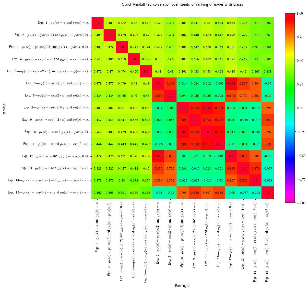
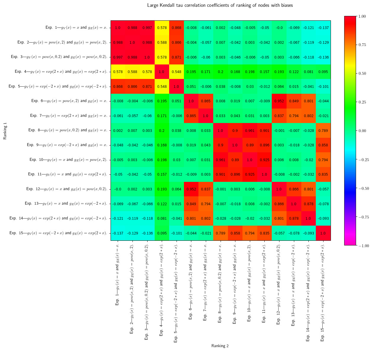
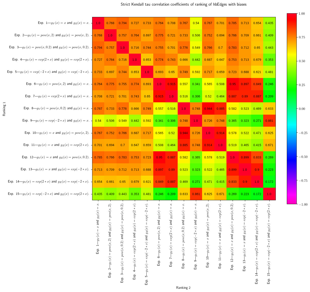
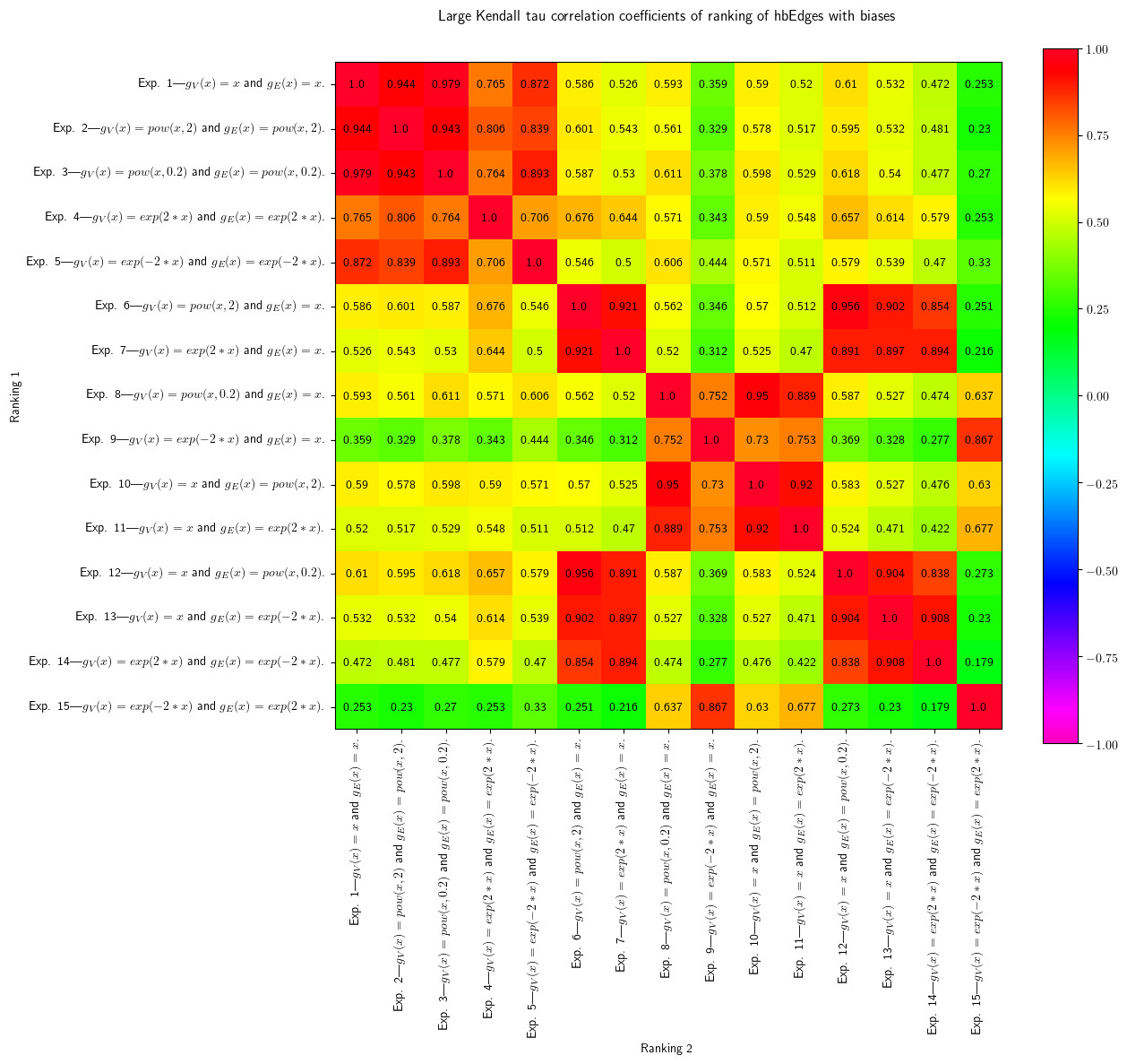
We compare the rankings obtained on vertices and hb-edges after 200 iterations of the exchange-based diffusion using the strict and large Kendall tau correlation coefficients for the different biases proposed in Table 2. We present the results as a visualisation of correlation matrices in Figure 1 and in Figure 2, lines and columns of these matrices being ordered by the experiment index presented in Table 2.

We write $\sigma_{i,t}$ the ranking obtained with Experiment $i$ biases for $t\in\left\{V,E\right\}$ indicating whether the ranking is performed on vertices or hb-edges—the absence of $t$ means that it works for both rankings. The ranking obtained by Experiment 1 is called the reference ranking.

In Experiments 2 to 5, the same bias is applied to both vertices and hb-edges. In Experiments 2 and 3, the biases are increasing functions on $\left[0;+\infty\right[,$ while in Experiments 4 and 5, they are decreasing functions.

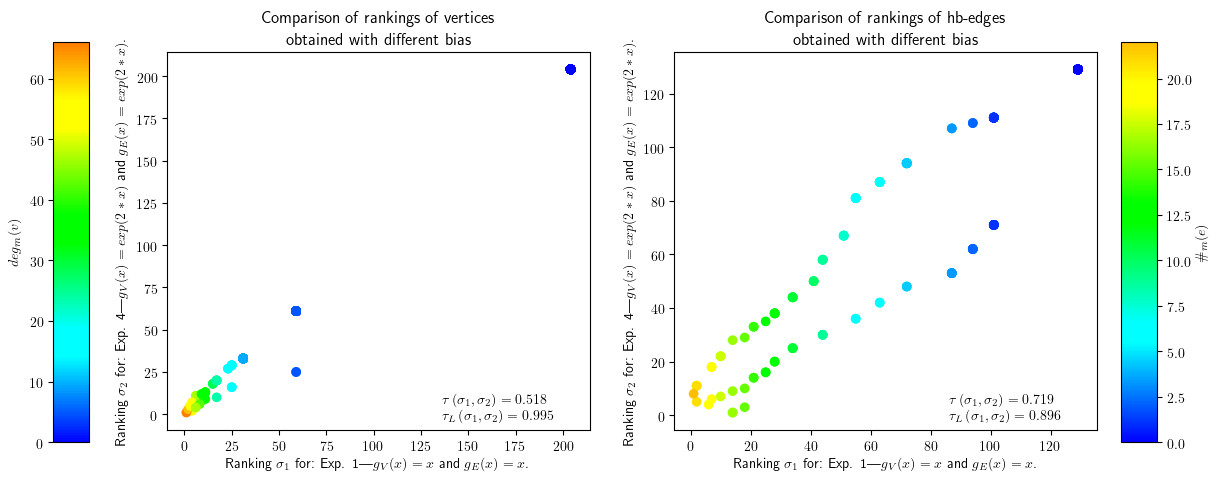
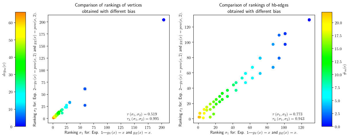
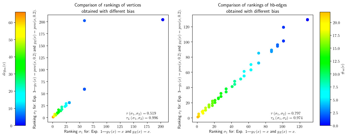
Experiments 2 and 3 lead to rankings that are well correlated with the reference ranking given the large Kendall tau correlation coefficient value. The higher value of $\tau_{L}\left(\sigma_{i},\sigma_{j}\right)$ compared to the one of $\tau\left(\sigma_{i},\sigma_{j}\right)$ marks the fact that the rankings with pair of similar biases agree with the ties in this case. The exponential bias yields to a ranking that is more granular in the tail for vertices, and reshuffles the way the hb-edges are ranked; similar observations can be done for both the vertex and hb-edge rankings in Experiments 2 and 3.

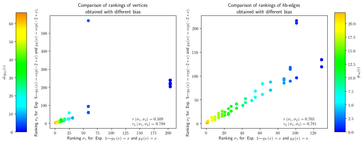
In Experiments 4 and 5, the rankings remain well correlated with the reference ranking but the large Kendall tau correlation coefficient values show that there is much less agreement on the ties, but it is very punctual in the rankings, with again more discrimination with an exponential bias. This slight changes imply a reshuffling of the hb-edge rankings in both cases, significantly emphasized by the exponential form.

None of these simultaneous pairs of biases reshuffle very differently the rankings obtained in the head of the rankings of vertices, but most of them have implications on the head of the rankings of the hb-edges: typical examples are given in Figure 3. It would need further investigations using the Jaccard index.

Dissimilarities in rankings occur when the bias is applied only to vertices or to hb-edges. The strict Kendall tau correlation coefficients between the rankings obtained when applying the bias of Experiments 6 to 9—bias on vertices—and 10 to 13—bias on hb-edges—and the reference ranking for the vertices show weak consistency for vertices with values around 0.4—Figure 1 (a)—, while the large Kendall tau correlation coefficient values show a small disagreement with values around -0.1—Figure 1 (b). For hb-edges, the gap is much less between the strict—values around 0.7 as shown in Figure 2 (a)—and large Kendall tau correlation coefficient values—with values around 0.6 as shown in Figure 2 (b).

Biases with same monotony variations—$g_{t}\left(x\right)=x^{2}$ and $g_{t}\left(x\right)=e^{2x}$ on the one hand and $g_{t}\left(x\right)=x^{0.2}$ and $g_{t}\left(x\right)=e^{-2x}$ on the other hand—have similar effects independently of their application to vertices xor to hb-edges. It is also worth to remark that increasing biases lead to rankings that have no specific agreement or disagreement with rankings of decreasing biases—as it is shown with $\tau_{L}\left(\sigma_{i},\sigma_{j}\right)$ and $\tau\left(\sigma_{i},\sigma_{j}\right)$ for $i\in\left\llbracket 6;13\right\rrbracket.$

We remark also that increasing biases applied only to vertices correlate with the corresponding decreasing biases applied only to hb-edges, and vice-versa. This is the case for Experiments 6 and 12, Experiments 7 and 13, Experiments 8 and 10, and Experiments 9 and 11 for both vertices—Figures 1 (a) and (b)—and hb-edges—Figures 2 (a) and (b).

Finally, we conduct two more experiments—Experiments 14 and 15—combining the biases $g_{t}\left(x\right)=e^{2x}$ and $g_{t}\left(x\right)=e^{-2x}$ in two different manners. With no surprise, they reinforce the disagreement with the reference ranking both on vertices and hb-edges, with a stronger disagreement when the decreasing bias is put on vertices. We can remark that Experiment 14—$g_{V}\left(x\right)=e^{2x}$ and $g_{E}\left(x\right)=e^{-2x}$—has the strongest correlations with the rankings of dissimilar biases that are either similar to the one of vertices—Experiments 6 and 7— or to the one of hb-edges—Experiments 12 and 13.

(a) Strict Kendall tau correlation coefficient

(b) Large Kendall tau correlation coefficient

Figure 1: Strict (a) and large (b) Kendall tau correlation coefficient for node ranking with biases. Realized on 100 random hb-graphs with 200 hb-edges of maximal size 20, with 5 groups.

(a) Strict Kendall tau correlation coefficient

(b) Large Kendall tau correlation coefficient

Figure 2: Strict (a) and large (b) Kendall tau correlation coefficient for hb-edge ranking with biases. Realized on 100 random hb-graphs with 200 hb-edges of maximal size 20, with 5 groups.

(a) First ranking: $g_{V}\left(x\right)=x$ and $g_{E}\left(x\right)=x$; Second ranking: $g_{V}\left(x\right)=e^{2x}$ and $g_{E}\left(x\right)=e^{2x}.$

(b) First ranking: $g_{V}\left(x\right)=x$ and $g_{E}\left(x\right)=x$; Second ranking: $g_{V}\left(x\right)=x^{2}$ and $g_{E}\left(x\right)=x^{2}.$

(c) First ranking: $g_{V}\left(x\right)=x$ and $g_{E}\left(x\right)=x$; Second ranking: $g_{V}\left(x\right)=e^{-2x}$ and $g_{E}\left(x\right)=e^{-2x}.$

(d) First ranking: $g_{V}\left(x\right)=x$ and $g_{E}\left(x\right)=x$; Second ranking: $g_{V}\left(x\right)=x^{0.2}$ and $g_{E}\left(x\right)=x^{0.2}.$

Figure 3: Effect of vertex biases on ranking.

A last remark is on the variability of the results: if the values of the correlation coefficients change, from one hb-graph to another, the phenomenon observed remains the same, whatever the first hb-graph observed; however, the number of experiments performed ensures already a minimized fluctuation in these results.

5 Further Comments

The biased-exchange-based diffusion proposed in this Chapter enhances a tunable diffusion that can be integrated into the hb-graph framework to tune adequately the ranking of the facets. The results obtained on randomly generated hb-graphs have still to be applied to real hb-graphs, with the known difficulty of the connectedness: it will be addressed in future work. There remains a lot to explore on the subject in order to refine the query results obtained with real searches. The difficulty remains that in ground truth classification by experts, only a few criteria can be retained, that ends up in most cases in pairwise comparison of elements, and, hence, does not account for higher order relationships.

References

• [1] X. Ouvrard, J.-M. Le Goff, and S. Marchand-Maillet, “Adjacency and Tensor Representation in General Hypergraphs. Part 2: Multisets, Hb-graphs and Related e-adjacency Tensors,” arXiv preprint arXiv:1805.11952, 2018.
• [2] X. Ouvrard, J.-M. Le Goff, and S. Marchand-Maillet, “Diffusion by Exchanges in HB-Graphs: Highlighting Complex Relationships Extended version,” Arxiv:1809.00190v2, 2019.
• [3] X. Ouvrard, J.-M. Le Goff, and S. Marchand-Maillet, “On Hb-graphs and their Application to General Hypergraph e-adjacency Tensor,” MCCCC32 Special Volume of the Journal of Combinatorial Mathematics and Combinatorial Computing, to be published, 2019.
• [4] M. Dehmer and A. Mowshowitz, “A history of graph entropy measures,” Information Sciences, vol. 181, pp. 57–78, Jan. 2011.
• [5] V. Zlatic, A. Gabrielli, and G. Caldarelli, “Topologically biased random walk and community finding in networks,” Physical Review E, vol. 82, p. 066109, Dec. 2010.
• [6] X. Ouvrard, J.-M. Le Goff, and S. Marchand-Maillet, “Diffusion by Exchanges in HB-Graphs: Highlighting Complex Relationships,” CBMI Proceedings, 2018.