HST/STIS transmission spectrum of the ultra-hot Jupiter WASP-76 b confirms the presence of sodium in its atmosphere

We present an atmospheric transmission spectrum of the ultra-hot Jupiter WASP-76 b by analyzing archival data obtained with the Space Telescope Imaging Spectrograph (STIS) on board the Hubble Space Telescope (HST). The dataset spans three transits, two with a wavelength coverage between 2900 and 5700 Å, and the third one between 5250 and 10300 Å. From the one-dimensional, time dependent spectra we constructed white and chromatic light curves, the latter with typical integration band widths of $\sim$200 Å. We computed the wavelength dependent planet-to-star radii ratios taking into consideration WASP-76’s companion. The resulting transmission spectrum of WASP-76 b is dominated by a spectral slope of increasing opacity towards shorter wavelengths of amplitude of about three scale heights under the assumption of planetary equilibrium temperature. If the slope is caused by Rayleigh scattering, we derive a lower limit to the temperature of $\sim$870 K. Following-up on previous detection of atomic sodium derived from high resolution spectra, we re-analyzed HST data using narrower bands centered around sodium. From an atmospheric retrieval of this transmission spectrum, we report evidence of sodium at 2.9$\sigma$ significance. In this case, the retrieved temperature at the top of the atmosphere ($10^{-5}$ bar) is $2300^{+412}_{-392}$ K. We also find marginal evidence for titanium hydride. However, additional high resolution ground-based data are required to confirm this discovery.

1 Introduction

Transiting exoplanets allow us to study their atmospheres and determine their physical and chemical properties through transmission spectroscopy, and to do so we analyze the light of their host stars filtered through their atmospheres. This technique has been used to detect several atomic and molecular species in exoplanetary atmospheres, as for example sodium on HAT-P-1 b (Nikolov et al., 2014), sodium and potassium on WASP-103 b (Lendl et al., 2017), WASP-39 b (Fischer et al., 2016) and WASP-127 b (Chen et al., 2018), H₂O and CO on HD 209458 b (Deming et al., 2013), H₂O on WASP-19 b (Huitson et al., 2013) and HAT-P-32 b (Damiano et al., 2017), VO on WASP-121 b (Evans et al., 2018), and clouds and hazes on HD 189733 b (Sing et al., 2011), HAT-P-18 b (Kirk et al., 2017), WASP-49 b (Lendl et al., 2016), and WASP-6 b (Nikolov et al., 2015). It was Charbonneau et al. (2002) who first observed an exoplanetary atmosphere on HD 209458 b via the detection of atmospheric neutral sodium at 5980 Å with the Space Telescope Imaging Spectrograph (STIS) mounted on the Hubble Space Telescope (HST). Since then, transmission spectroscopy, space-based and ground-based, has been widely used to characterize exo-atmospheres (see e.g., Sing et al., 2016; Tsiaras et al., 2018, for comparative studies of large samples of exoplanets).

Ultra-hot Jupiters are a population of planets that have day-side temperatures higher than $\sim$2200 K and a large thermal difference between their hemispheres, thereby offering excellent conditions for detailed studies of the physics and chemistry of their atmospheres (Parmentier et al., 2018). Due to the extreme atmospheric temperatures these exoplanets are expected to be more diverse when compared to hot Jupiters. So far, ultra-hot Jupiters that were discovered by transit surveys presenting inflated radii are more likely to be found orbiting hot stars (see e.g., Hartman et al., 2016). It was with the interest in knowing more about these worlds that West et al. (2016) first announced and further examined WASP-76 b, an inflated ultra-hot Jupiter orbiting each $\sim$1.8 days a main sequence star of $\sim$6200 K. The optical transit depth of WASP-76 b is $\sim$1.2%, but if the planet was not inflated it would merely be $\sim$0.36%. This translates into a large scale height, of approximately 1250 km above the nominal planet radius. Comparing WASP-76 b to other exoplanets in their mass versus incident flux, it is clear that WASP-76 b has a higher incident flux than other exoplanets of the same mass, which could in principle explain its inflated radius.

The ultra-hot Jupiters that were studied to a good level of detail so far seem to show a large spread of features. For example, WASP-12 b shows a Rayleigh slope with an amplitude of $\sim$2 scale heights (Stevenson et al., 2014). Hoeijmakers et al. (2019) found heavy metals in one of the hottest exoplanets known to date, KELT-9 b. The controversial WASP-19 b shows either titanium oxide (Sedaghati et al., 2017) or a flat spectrum (Espinoza et al., 2019). Aluminium oxide was discovered in the atmosphere of WASP-33 b (von Essen et al., 2019), and WASP-121 b revealed magnesium and iron absorption at UV wavelengths, absorption of a currently unknown source at short optical wavelengths and indications for VO (Evans et al., 2018). Lendl et al. (2017) detected sodium and potassium on WASP-103 b, and interpreted its atmosphere as potentially cloud-free. A recent study carried out by Seidel et al. (2019); Žák et al. (2019) report on the detection of neutral sodium in the atmosphere of WASP-76 b, obtained analyzing high resolution spectra. In particular, Seidel et al. (2019) found the sodium lines to be significantly broadened, and they speculate this broadening to be an indicator of super-rotation in the upper atmosphere of WASP-76 b.

In this work, we present the characterization of the atmosphere of WASP-76 b from the near UV to the near IR, obtained analyzing three primary transits using archival data of HST/STIS. This article is structured as follows. In Section 2 we present the observations and the data reduction, and then give a detailed description of the model parameters and fitting process in Section 3. In Section 4 we show our results on the transmission spectrum of WASP-76 b, we determine the impact of third light contamination into our transmission spectrum in Section 4.1, we investigate some mechanisms that could mimic the derived slope in detail in Section 5, we discuss our results in Section 6, and we finalize with some concluding remarks in Section 7.

2 Data log and data preparation

For this work we used archival data provided in the Mikulski Archive for Space Telescopes (Proposal ID 14767). Two transits of WASP-76 b were observed during the 16^th of November, 2016, and the 17^th of January, 2017. These data sets were collected using the HST STIS G430L grating. A third transit was observed on the 19^th of February, 2017, but this time with the G750L grating. The G430L data set consists of 164 spectra spanning the two transits covering the wavelength range between 2900 and 5700 Å. The G750L data set consists of 81 spectra covering the wavelength range between 5250 and 10300 Å. Each transit spans five spacecraft orbits, and the visits are such that the third and fourth spacecraft orbits contain the center of the transit, which provides good coverage between second and third contact, as well as an out-of-transit baseline before and after the transit. The exposure time is fixed to 140 seconds in all cases, and the timestamp of each exposure is converted to Barycentric Julian Dates using the mid-time of the exposure and Eastman et al. (2010)’s tool.

During the reduction process we cleaned the data from cosmic ray hits using the cosmicrays task in IRAF, which locates and removes cosmic rays using statistical modelling (Wells & Bell, 1994). As this IRAF task is usually used and thought to work on images of stars rather than spectral images, we carried out a detailed process of cosmic ray extraction. Here, we divided one of our spectral images into three images, one image containing most of the light along the spectral trace, and two images containing the background, above and below the trace. The two images containing the background should only have light from cosmic rays, and we can thus identify the pixels contaminated from cosmic rays without confusing them with pixels containing light from the star. We used these images to train the selection criteria in the cosmicrays task, as the input parameters are fundamental for the success of the extraction.

To determine the spectral trace we used IRAF’s task APALL, with pixel-dependent polynomials which order ranged from first to tenth. An eight order polynomial was finally chosen, as this minimized the residuals of the fitted trace. Following von Essen et al. (2019), we used the background subtraction that comes with the APALL task. The function for removing the background was set to second order and the predefined background regions were set to be as far away from the spectral trace as possible ($\sim$ 50 pixels/20 full width at half maximum, FWHM) while still having a substantial width containing purely background, of $\sim$10 pixels at each side of the spectral trace. Following the example of Huitson et al. (2013) and von Essen et al. (2019), the aperture extraction was performed using APALL. First, we extracted fluxes using several apertures, specifically from 10 to 50 pixels in steps of 1 pixel. Then, we produced white transit light curves (this is, light curves produced integrating fluxes in all wavelengths) and we computed the standard deviation of the off-transit data points. As final aperture we chose the one minimizing this standard deviation. The final apertures were fixed to 19 pixels for the G430L grating, and 43 pixels for the G750L grating. Our final aperture sizes include WASP-76’s companion (see e.g., Wöllert & Brandner, 2015; Ngo et al., 2016). The adequate treatment for third light contamination that we carry out to correctly derive the transmission spectrum of WASP-76 b is detailed in Section 4.1.

The STIS spectra were used to create both a white light photometric time series, where the flux is integrated over all wavelengths for each exposure, and chromatic light curves, where custom wavelength bands were chosen, integrating the flux in each wavelength bin for each exposure. The resulting light curves exhibit all the expected instrumental effects other authors have also encountered (Sing et al., 2011, 2015; Huitson et al., 2013; Nikolov et al., 2014, 2015), though first described by Brown et al. (2001), and we follow their example to handle them. The main instrument related systematic effect is due to the thermal breathing of HST, which warms and cools the telescope during its $\sim$96 min day/night cycle (Sing et al., 2013). This results in changes in the point spread function and in the central position of the spectrum. This was accounted for by fitting a fourth order polynomial phased to the HST period to the fluxes, in simultaneous to the transit model. As carried out by other authors, we also included in our detrending model a linear slope in time. Although this was our final detrending model setup, we also tried a second and third order polynomial phased to the HST period, a second order polynomial as a function of time, and a linear combination between the time-dependent spatial and wavelength shifts of the spectra (see Section 3.2), combining them in all possible ways. Our final detrending choice is favoured by the minimization of the Bayesian Information Criterion, BIC = $\chi^{2}$ + k ln N, where k is the number of model parameters, $\chi^{2}$ is computed between data and sub-models, and N is the number of data points.

When the telescope is moved to a new pointing position it takes approximately one spacecraft orbit to thermally relax, which compromises the stability of the first orbit (Huitson et al., 2013). In our first analysis we tried to keep the first orbit, but found that our detrending was not satisfactory, as a fourth order polynomial could not remove the large systematic trends. Therefore, we did not consider the first orbit of each transit during our analysis. For STIS it is also known that the first exposure of each spacecraft orbit is significantly fainter than the remaining exposures. To bypass this problem, Sing et al. (2011, 2015); Huitson et al. (2013); Nikolov et al. (2014, 2015) have set the exposure time of the first exposure to only 1 second. The main idea is to discard this exposure without suffering from a significant loss of valuable observing time. The observations analyzed in this work were obtained using this observing strategy.

For our transit light curves we computed the individual spectro-photometric errors following von Essen et al. (2017). For this end, we used the formalism provided by IRAF’s photometric errors, i.e.,

$$\epsilon^{2}=\frac{F/g+A\sigma^{2}+(A^{2}\sigma^{2})/N}{F},$$ (1)

where F is the integrated flux inside the wavelength band and aperture, A is the area inside the band and aperture, $\sigma$ is the standard deviation of the background, N the number of pixels in the background, and g is the gain of the detector. As also pointed out by von Essen et al. (2017), errors produced in this fashion are often underestimated, as they follow a photon-noise-only distribution, which is most likely unrealistic. We therefore scaled our errors with the standard deviation of the residual light curves. These were obtained subtracting to the fluxes a first model obtained from a quick least-squared fit.

3 Data modelling and fitting parameters

3.1 Transit model and limb darkening coefficients

The light curves were modelled using Mandel & Agol (2002). Here, the model parameters are the orbital inclination, i, the mid-transit time, T₀, the orbital period, P, the semi-major axis in stellar radii, $\mathrm{a/R_{s}}$, the planet-to-star radius ratio, $\mathrm{R_{P}/R_{S}}$, the third light contribution, described as the flux ratio between the stellar companion and the main star, and the limb darkening coefficients corresponding to a quadratic limb-darkening law:

$$\frac{I(\mu)}{I(1)}=1-a(1-\mu)-b(1-\mu)^{2},$$ (2)

where $I(1)$ is the specific intensity at the centre of the stellar disk, $a$ and $b$ are the linear and quadratic limb darkening coefficients (LDCs), respectively, and $\mu=\cos(\gamma)$, where $\gamma$ is the angle between the line of sight and the emergent intensity. We chose the simplest law as the differences in transit shape between a quadratic and a four-parametric non-linear limb darkening law are beyond the precision of our data (see e.g, Sotzen et al., 2020, for a similar choice). Nonetheless, we would like to emphasize that the precision given by limb-darkening coefficients only reflects the precision in the fit between stellar intensity models and the limb darkening model (von Essen et al., 2017), regardless of the choice of law. It does not reflect the real accuracy at which we know the radial profiles of stellar intensities (see e.g., White et al., 2013; Boyajian et al., 2015; Kervella et al., 2017), reason why we disbelieve in applying changes that might have an impact in the third or fourth decimal of the limb-darkening coefficients, as these would not be supported by our knowledge on stellar physics. To calculate the customized LDCs for each wavelength bin, we used angle-dependent, specific intensity spectra from PHOENIX (Göttingen, 2018) with main stellar parameters corresponding to the effective temperature, $\mathrm{T_{eff}}$ = 6200 K, the surface gravity, log(g) = 4.5, and the metallicity, [Fe/H] = 0.00, closely matching the values of WASP-76, which are $\mathrm{T_{eff}}$ = 6250 K, log(g) = 4.4 (Seidel et al., 2019) and [Fe/H] = 0.19 (Brown et al., 2017). As performed by von Essen et al. (2017) and Claret & Bloemen (2011), to compute the limb darkening coefficients we neglect the data points at small $\mu$’s, specifically those between $\mu$ = 0 and $\mu$ = 0.064. The uncertainties of the linear and quadratic LDCs are obtained from $\chi^{2}$ maps, specifically choosing the values of the LDCs at which $\Delta\chi^{2}$ = 1. All the LDCs used for the chromatic light curves are presented in Table 4.

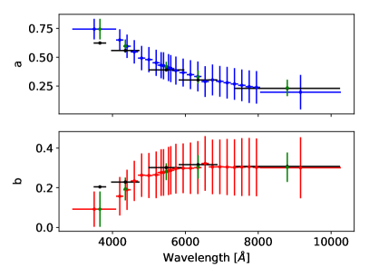
To assess the quality of our procedure, we compared our LDCs with the ones computed by Claret (2000) and Claret & Bloemen (2011) for the Johnson-Cousins $U$, $B$, $V$, $R$ and $I$ filters. A comparison between LDCs can be seen in Figure 1. In the figure, the blue and red data points are our calculated LDCs for each wavelength bin for the linear, $a$, and quadratic, $b$, coefficients specified in Equation 2. The horizontal lines represent the width of the bins, and the vertical lines show the uncertainty on each LDC. To compare our costumed LDCs with those computed by Claret (2000) and Claret & Bloemen (2011) for the $UBVRI$ filters, we compute averages and errors of those LDCs contained within the FWHM of each broad band filter. The derived values are shown in the Figure in green. The best match between our customized LDCs and published ones comes from the values reported by Claret & Bloemen (2011), shown in black in Figure 1. The resulting values are presented in Table 1. Claret & Bloemen (2011) does not provide uncertainties. In consequence, these are absent in the Table and the Figure. As Figure 1 reveals, ours and Claret & Bloemen (2011)’s LDCs match at all wavelengths considering 1-$\sigma$ uncertainties. It is worth to mention that the errors provided in this work are merely statistical, and do not realistically reflect the accuracy at which we know any limb-darkening coefficients.

Table 1: LDCs for the $U$, $B$, $V$, $R$ and $I$ filters obtained from Claret & Bloemen (2011) (C11), and computed in this work (TW). The coefficients, a and b, correspond to those in equation 2.

	$U$	$B$	$V$	$R$	$I$
$a_{\mathrm{C11}}$	0.6234	0.5578	0.3898	0.3021	0.2296
$a_{\mathrm{TW}}$	0.7442 $\pm$ 0.0889	0.5971 $\pm$ 0.1704	0.4188 $\pm$ 0.3287	0.3280 $\pm$ 0.2875	0.2340 $\pm$ 0.2850
$b_{\mathrm{C11}}$	0.2043	0.2286	0.3013	0.3162	0.3069
$b_{\mathrm{TW}}$	0.09210 $\pm$ 0.0889	0.1936 $\pm$ 0.1727	0.2807 $\pm$ 0.3387	0.3048 $\pm$ 0.2965	0.3031 $\pm$ 0.2950

Figure 1: Computed limb darkening coefficients (LDCs) for the chromatic light curves in red (linear LDC) and blue (quadratic LDC), compared to the LDCs for the $UBVRI$ filters taken from Claret & Bloemen (2011) in black. In all cases, horizontal lines correspond to the width of the integration band for the custom wavelength bins, and the FWHM for the broad band filters. The green dots represent average values of the LDCs computed in this work, coinciding with the wavelength coverage of each of the $UBVRI$ filters. The vertical lines show their uncertainties.

3.2 Detrending model

HST light curves show non-Gaussian, correlated noise (see Section 2). In consequence, as previously done (Sing et al., 2011, 2015; Huitson et al., 2013; Nikolov et al., 2014, 2015), we apply orbit-to-orbit flux corrections by fitting a fourth degree polynomial phased to the orbit of HST (henceforth, model M4) to account for the thermal breathing of HST, and a linear slope (henceforth, model M1) in time. The resulting detrending function is described as follows:

$$\begin{split}f(t)=&\leavevmode\nobreak\ (a_{0}+a_{1}\cdot x+a_{2}\cdot x^{2}+a_{3}\cdot x^{3}+a_{4}\cdot x^{4})\\ &\cdot(c_{0}+c_{1}\cdot(t-T_{0})),\end{split}$$ (3)

where $a_{0},a_{1},a_{2},a_{3}$ and $a_{4}$ are the detrending coefficients for the fourth degree polynomial, and $c_{0}$ and $c_{1}$ are the detrending coefficients for the linear slope. In addition, $t$ is the time, $T_{0}$ is the mid-time of the transits, and:

$$x_{i}=\frac{t_{i}-t_{0}}{\mathrm{per_{HST}}}-\mathrm{int}\left(\frac{t_{i}-t_{0}}{\mathrm{per_{HST}}}\right).$$ (4)

Here, $t_{0}$ corresponds to the first time stamp for each transit, and per_HST corresponds to the period of HST’s orbit. These functions are fitted simultaneously to the transit model.

Earlier studies using HST data (see e.g., Sing et al., 2011, 2013; Huitson et al., 2013) have also included systematic trends which correlate with the X and Y detector positions of the spectra. To analyze if this was necessary, we computed both X (model X, MX) and Y (MY) shifts. First, we determined the shift in the Y detector position by fitting multiple Gaussian functions to the stellar spectrum in its spatial direction. The reference position of the trace per X pixel is represented by the mean of the Gaussian function. For this exercise we considered the first spectral exposure of each transit to be the reference spectrum, and found the shift in the spectral trace by comparing the other spectra to this, making one-to-one differences of these mean values, that were afterwards averaged. Then, we computed the shift in X detector position by selecting 3 deep absorption lines from the stellar spectra. To each one of these lines we fitted a Gaussian function, and used their means as central wavelength positions. Equivalently to the Y shifts, we chose the first frame as the reference one. Computing one-by-one differences between the line centers of the reference frame and the subsequent spectral exposures, and averaging these differences in time, we determined the X shifts. To quantify to which extent were the chromatic light curves affected by the X and Y detector positions of the spectral traces, we made use of the Pearson correlation coefficient (PCC), computed between our residuals and the X and Y trends determined as just explained. After finding no strong correlation between these pairs (PCC$<$0.2 in all cases), we decided not to include these components in the detrending model. This choice was also supported making use of the BIC. In Table 2 we list some of the most relevant detrending models and their corresponding BIC values, obtained averaging the BIC’s computed from each one of the three white light curves. Besides the BIC minimization, in this work we have considered $\Delta$BIC $<$ -5 between two given models as strong evidence to which model is more likely (Kass & Raftery, 1995).

Table 2: BIC minimization computed considering different detrending models. From left to right the detrending model, the number of detrending parameters fitted in each case, NDP, and the Bayesian Information Criterion (BIC).

Model	NDP	BIC
(1) M1	2	178.5
(2) M4	5	164.2
(3) M1 $\times$ M4	7	137.9
(4) M1 $\times$ M4 $\times$ MX	8	142.3
(5) M1 $\times$ M4 $\times$ MY	8	143.1
(6) M1 $\times$ M4 $\times$ (MX + MY)	9	143.7

3.3 Generalities on our fitting procedure

As carried out by von Essen et al. (2019), to derive the model parameters we fitted all the light curves simultaneously using Markov-chain Monte Carlo (MCMC), all wrapped up in PyAstronomy (Patil et al., 2010; Jones et al., 2001). For both white (flux integrated in all wavelengths) and chromatic (flux integrated in narrow wavelength bands) light curves, we carried out our parameter fitting procedure in two stages. The first stage was carried out specifically to quantify the amount of correlated noise in our light curves, in order to determine reliable spectro-photometric error bars. The second stage was carried out to determine reliable error bars for the fitting parameters, using enlarged photometric error bars that accounted for correlated noise.

In general, the iterations used for the white light curves are 200 000 and 1 000 000 for the first and second stages, respectively, with a burn in of the initial 20% samples. Equivalently, for the chromatic light curves we iterated 400 000 and 500 000 times, with a burn-in of the initial 100 000 samples. From the posterior distributions we computed the mean and standard deviation (1-$\sigma$), and used them as our best-fit values and uncertainties, respectively. The MCMC chains were checked for convergency by visual inspection, which in turn was used to set the burn-in. We also divided the chains in three sub-chains, and computed from each one of them the usual statistics. We considered a chain to converge if the derived parameters were consistent between each other at 1-$\sigma$ level.

Finally, we chose the starting values for our MCMC chains during the first stage to be the ones specified in Table 3, adopted from Seidel et al. (2019). The uncertainty in the Gaussian priors were set to be three times the author’s uncertainties for each parameter. For the second stage we used the best-fit values from the first run, considering uncertainties at a 3-$\sigma$ level.

3.4 First MCMC run: correlated noise

To compute the amount of correlated noise in our light curves, we followed the methods of von Essen et al. (2013). To do so, we computed residuals from our first MCMC fit, subtracting the transit-times-detrending model from our transit light curves. As each HST orbit takes about 45 minutes and the ingress/egress duration of WASP-76 b is approximately half of that, we divided each HST orbit into 2 bins of equal duration (M = 2$\times$4 orbits = 8), and calculated the number of points in each bin, N. If the data are not affected by correlated noise, they should follow the expectation of independent random numbers,

$$\sigma_{N}=\sigma_{1}N^{-1/2}[M/(M-1)]^{1/2},$$ (5)

where $\sigma_{1}$ is the variance of the unbinned data, and $\sigma_{N}$ is the variance of the binned data, with the following expression:

$$\sigma_{N}=\sqrt{\frac{1}{M}\sum^{M}_{i=1}(\langle\hat{\mu}_{i}\rangle-\hat{\mu}_{i})^{2}}.$$ (6)

Here, $\hat{\mu}_{i}$ is the mean value of the residuals per bin, and $\langle\hat{\mu}_{i}\rangle$ is the mean value of all the means. If the data are affected by correlated noise, each $\sigma_{N}$ value would differ by a factor of $\beta_{N}$ from their expectation value. $\beta$ is an estimation of the strength of the correlated noise computed from averaging certain $\beta_{N}$’s, so a $\beta=1$ means no correlated noise. As we chose to divide each HST orbit only in two, $\beta_{N}=\beta$. We finally increased the size of the error bars by this factor. To place our results in context with other work, Nikolov et al. (2014) find $\beta$ values of 1.2 and 1.3 in their white light curves for observations carried out with the G430L grating, and a $\beta$ of 1 for observations with the G750L grating. Evans et al. (2018) find $\beta$ values of 1.29, 1.16, and 1.36 for the same gratings. Our computed $\beta$ values are 1.35, 1.30 and 1.55, respectively.

3.5 Second MCMC run: best-fit parameters and uncertainties

For all the light curves the central transit time, T₀, the semi-major axis in units of stellar radius, a/$\mathrm{R_{s}}$, the orbital inclination, i, the planet-to-star radius ratio, $\mathrm{R_{p}/R_{s}}$, and the detrending parameters specified in Equation 3 were fitted simultaneously. As T₀, a/$\mathrm{R_{s}}$, and i are values that are wavelength-independent, we treated them as equal for all the white and chromatic light curves. In other words, we only fitted one of each parameter for all the wavelength bins and the three light curves combined. Contrary to this, the $\mathrm{R_{p}/R_{s}}$ parameters were treated as equal in each wavelength bin for the two transits in the G430L grating, and differently in different wavelength bins. All the detrending parameters and $\mathrm{R_{p}/R_{s}}$ have uniform priors. The transit parameters T₀, a/$\mathrm{R_{s}}$, and i have Gaussian priors, as we know these from Seidel et al. (2019). We also use the value from Seidel et al. (2019) for the period, but we considered the orbital period as fixed, as it is known with a very high degree of precision and, in consequence, will have a negligible impact in our light curve fitting.

4 Results

4.1 Third light of another star in the aperture

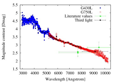
If there is a companion whose light falls into the photometric aperture, its third light contamination modifies the transit depth of the planet. When the companion is of later spectral type than the planet host, the third light contribution becomes stronger toward longer wavelengths. That means, the dilution of the transit depth strengthens towards redder wavelengths, the derived apparent planet-star radius becomes smaller, thus it might mimic a scattering slope in the transmission spectrum (Southworth & Evans, 2016; Mallonn & Strassmeier, 2016). In the case of WASP-76, there is a well characterized companion with a separation of $\sim$0.4 arcseconds. Considering STIS plate scale, this translates into approximately 8 pixels. Some literature values of its magnitude contrast relative to WASP-76, coinciding with STIS G750L wavelength range, are 2.58 $\pm$ 0.27 mag in the SDSS i’ band (Ginski et al., 2016), and 2.51 $\pm$ 0.25 mag and 2.85 $\pm$ 0.33 mag in the SDSS i’ and z’ band, respectively (Wöllert & Brandner, 2015).

Either while computing the transit depth from the white light curves (Section 4.2) or from the chromatic transits in Section 4.3, the third light treatment to the transit light curves is the same, and is described as follows. From the spectroscopic 2D images we can disentangle the two PSFs of WASP-76 and its companion, so computing the third light contribution directly from the spectra is straight forward to do. To compute the flux ratio between companion and star we proceeded similarly to Mallonn & Strassmeier (2016). Per wavelength element we produced a cut in the spatial direction. To this profile, we fitted the sum of two Gaussian functions with same standard deviation using least-square minimization. The final third light contribution is nothing more than the ratio between the integrated fluxes of each star, weighted by each Gaussian profile. To increase the signal-to-noise of our wavelength-dependent third light contribution, we reproduced this process over each one of the available spectra. Finally, we averaged in the wavelength direction. Figure 2 shows our derived third light contribution in $\Delta$mag, compared to literature values (Wöllert & Brandner, 2015; Ginski et al., 2016). Even though our computation was performed independently per grating and image, there is a perfect overlap between the two gratings, and between the data sets of the two transits in the G430L grating. As the figure reveals, the magnitude contrast quickly increases with the increase in wavelength, which is typical of a companion of late spectral type.

From the derived wavelength-dependent contamination, for a specific chromatic light curve we computed the third light contribution from the weighted mean within each wavelength bin, using as weight the flux of WASP-76 alone, which in turn was also obtained averaging the fluxes of all available spectra. In this way, values where WASP-76’s flux is larger, have a higher weight. The third light contribution considered in our transit fitting is plotted in Figure 2 with black squares.

Figure 2: Third light contribution of WASP-76’s companion in $\Delta$mag as a function of wavelength. Blue filled circles correspond to the values derived from the G430L grating, while red empty circles belong to the G750L grating. In green squares we show literature values found in Wöllert & Brandner (2015) and Ginski et al. (2016). Uncertainties for the magnitudes are given at 1-$\sigma$ level. In black squares we show our flux-weighted third light contribution. Horizontal bars show either the filter FWHM or the width of the integration band.

4.2 White light curve

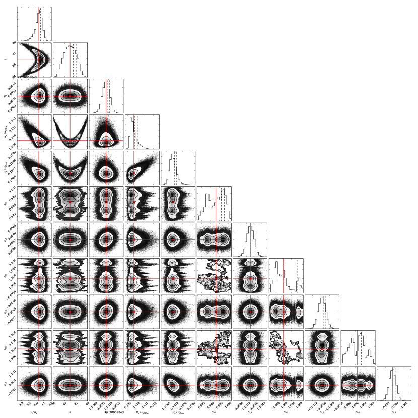
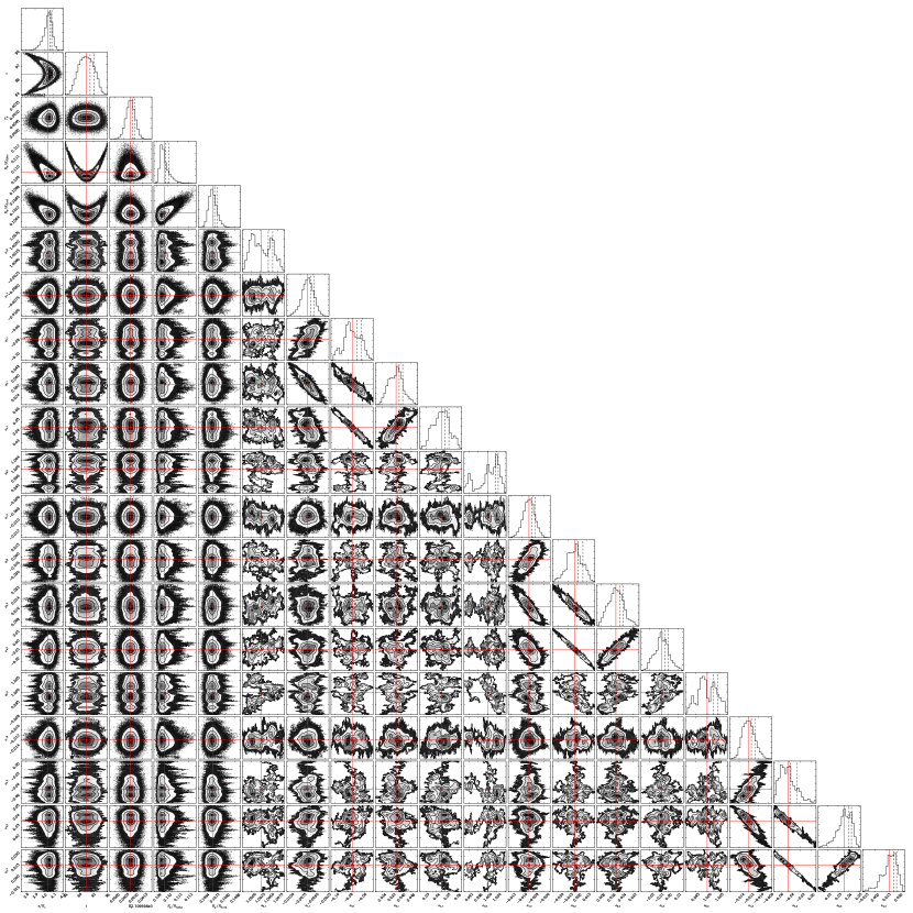
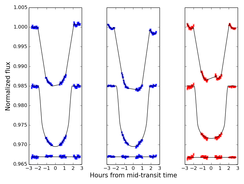
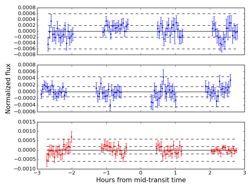
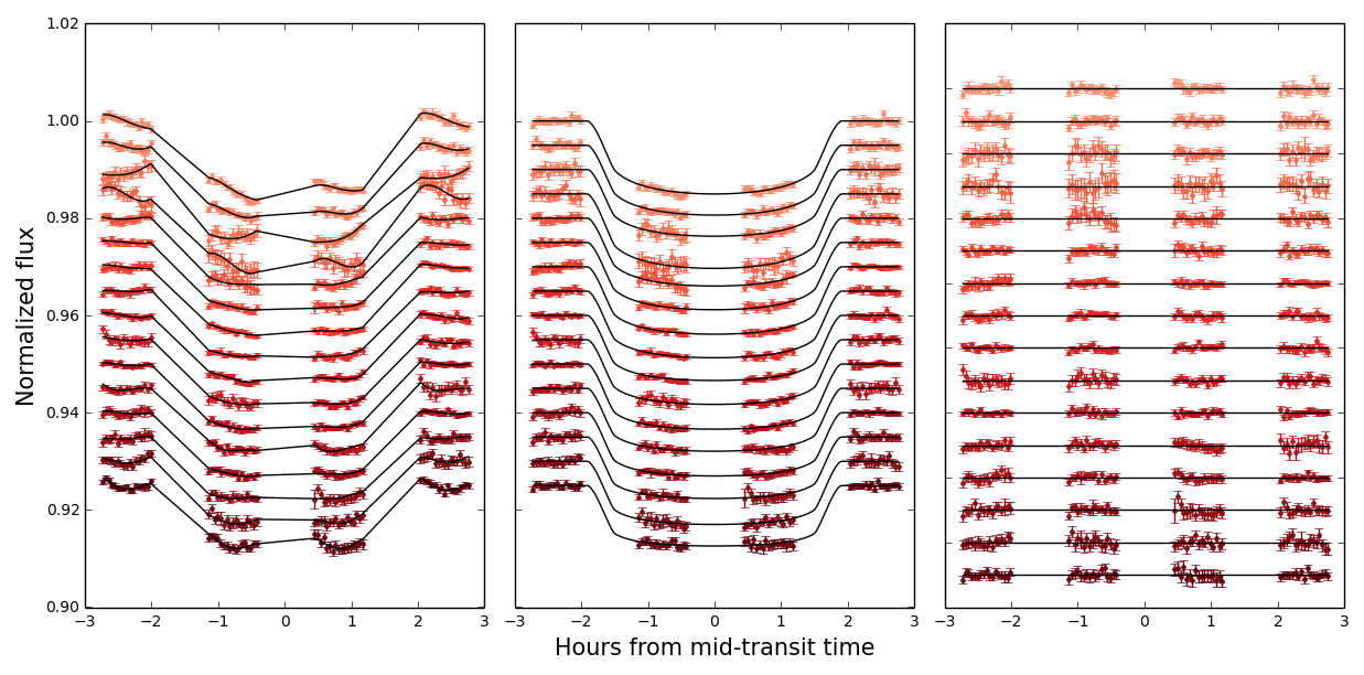
For our white light curves we integrated the light over all wavelengths for each exposure. For the G430L grating the specific wavelength range is from 2900 to 5700 Å, and for the G750L grating the wavelength range is from 5250 to 10300 Å. Our white light curves are presented in Figure 3, left, both containing the raw photometry with the systematic noise on the top, the detrended light curves in the middle, and the residuals in the bottom. A zoom in to the residuals is shown in Fig. 3, right. In all cases, with continuous black lines we show our best-fit combined model on top (transit times detrending), and our best-fit transit model only in the middle of the figure. In addition, Table 3 shows our derived values for the transit parameters that were fitted in this work. For comparison, the values from West et al. (2016) and Seidel et al. (2019) are also shown. Their reported $\mathrm{R_{p}/R_{s}}$’s are computed considering the spectral bands 3872 - 6943 Å, 3900 - 6800 Å, and 5850.24 - 5916.17 Å, respectively. As the table reveals, our derived transit parameters, a/R_s and i, are consistent with previous work at 1-$\sigma$ level. Posterior distributions for some of the fitted parameters can be seen in Appendix A. To investigate the impact of our choice of detrending over the transit depth, Fig. 9 shows the correlations between the transit parameters and the coefficients for the linear slope, c₀ and c₁, Fig. 10 those between the transit parameters and the coefficients for the fourth degree polynomial, a₀, a₁, a₂, a₃ and a₄. Besides the very well documented correlation between semi-major axis and inclination seen in both figures, we computed the Pearson’s correlation coefficient:

$$r_{xy}=\frac{\sum_{i=1}^{n}\ (x_{i}-\mu_{x})(y_{i}-\mu_{i})}{[\sum_{i=1}^{n}\ (x_{i}-\mu_{x})^{2}\sum_{i=1}^{n}\ (y_{i}-\mu_{y})^{2}]^{1/2}}\,,$$ (7)

for $x$ the planet-to-star radius ratio and $y$ the different detrending parameters. For the linear slope case, the r_xy coefficients were found to be between -0.03 and 0.05, and for the fourth degree polynomial, between -0.05 and 0.04. As both cases reflect a low correlation, we did not investigate the impact of the detrending coefficients any further.

Figure 3: HST white light curves for the three transits, shifted to their individual mid-transit times and shown in hours. Blue transits correspond to those taken with the G430L grating, and red to the one collected with the G750L grating. Left: from top to bottom we show the transit light curves with the systematic effects, along with our best-fit combined model (transit times detrending), the detrended data along with our best-fit transit model, and the residual light curves after both components were subtracted. Right: zoom in to the residuals. Dashed horizontal lines indicate $\pm$1 and $\pm$3 times the standard deviation of the residuals to guide the eyes.

Table 3: Computed transit parameter values from the white light curves (WLC) compared to those from Seidel et al. (2019) and West et al. (2016). The wavelengths used to compute the transit light curves are different, so the corresponding $\mathrm{R_{p}/R_{s}}$’s are not to be compared. $\Delta\lambda$ indicates the wavelength range in which our white light curves were integrated.

	This work (WLC)	Seidel et al. (2019)	West et al. (2016)
$\mathrm{R_{p}/R_{s}}$	G430L: 0.11122 $\pm$ 0.00032	0.10824 $\pm$ 0.00081	0.1090 $\pm$ 0.0007
	G750L: 0.11026 $\pm$ 0.00029
a/RS	4.036 $\pm$ 0.032	4.08${}^{+0.02}_{-0.11}$	4.102 $\pm$ 0.062
i (∘)	88.21 $\pm$ 0.95	86.72${}^{+1.72}_{-1.18}$	88.0${}^{+1.3}_{-1.6}$
T0 (BJDTDB)	7709.59863 $\pm$ 0.00012	8080.62487 $\pm$ 0.00018	6107.85507 $\pm$ 0.00034
$\Delta\lambda$ (Å)	G430L: [2900-5700] -
	G750L: [5250-10300]

4.3 Transmission spectrum of WASP-76 b

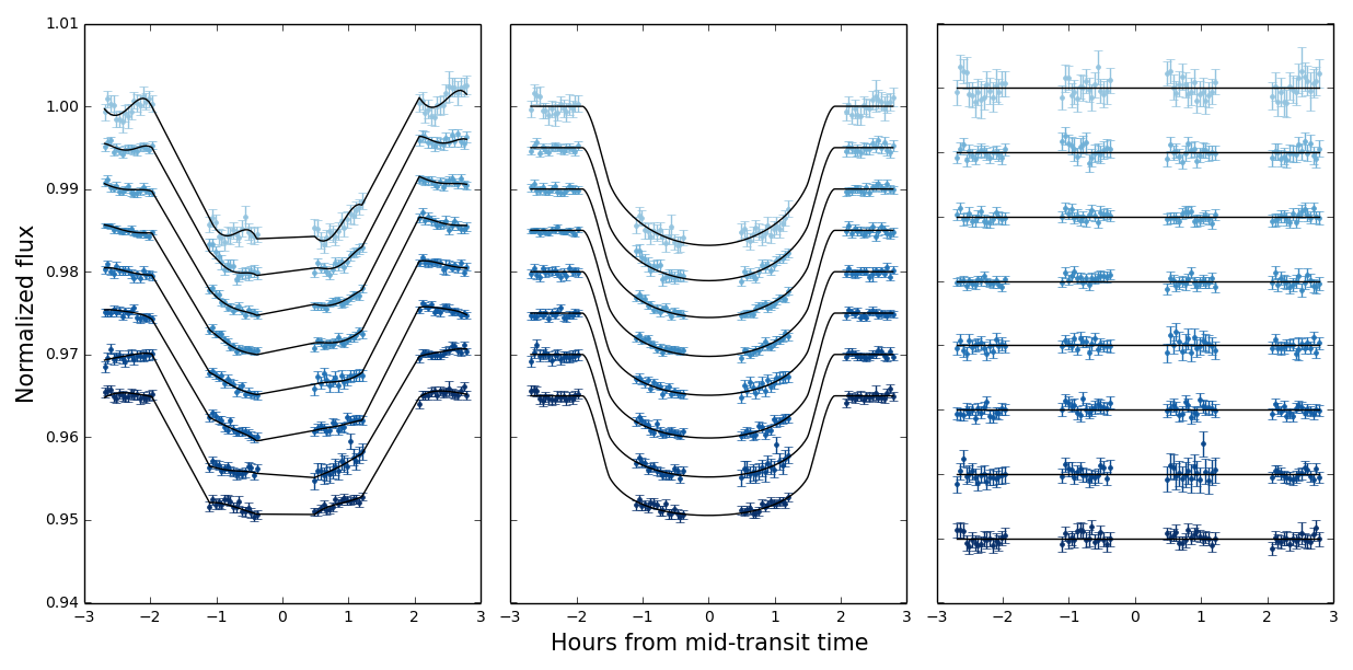
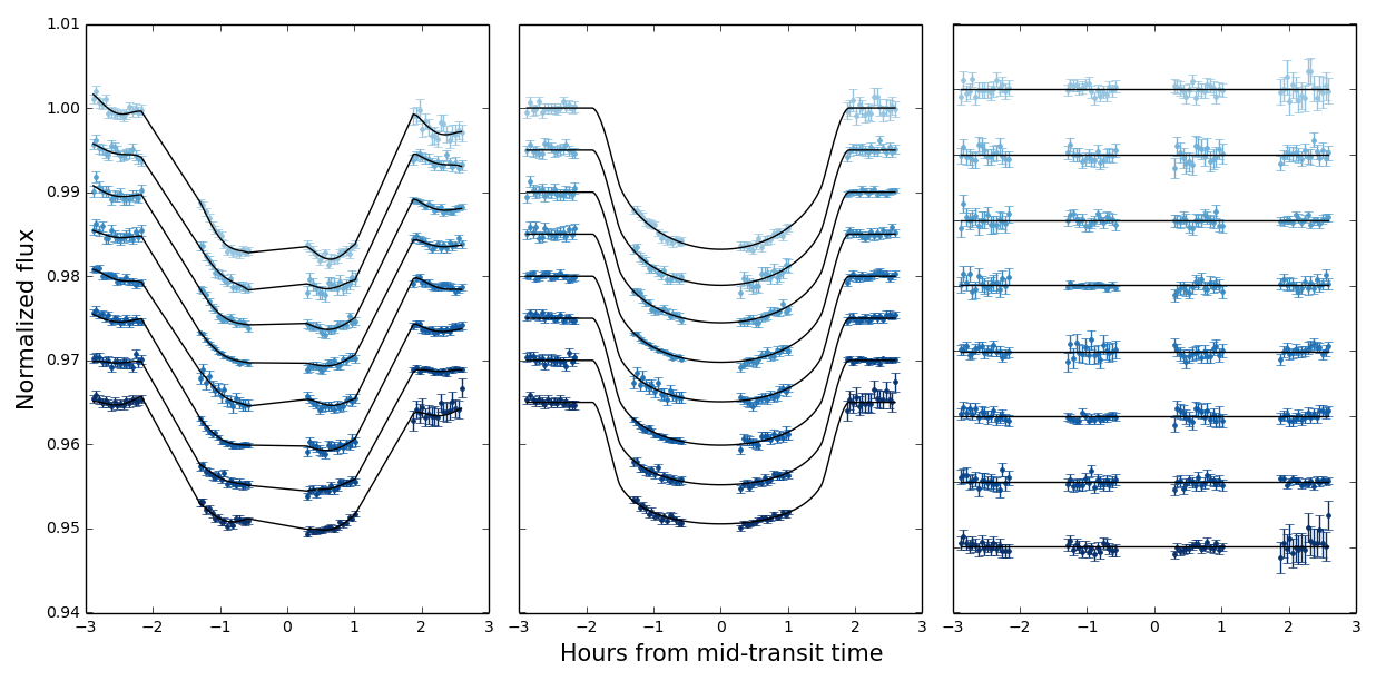
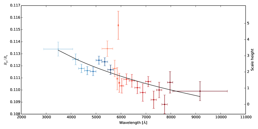
Initially, the spectra were divided into eight and thirteen wavelength bins for the blue and red gratings, respectively, and the $\mathrm{R_{P}/R_{S}}$ were computed for each bin. After Seidel et al. (2019)’s work, we recomputed the transmission spectrum in the same way, but choosing three narrow bands around sodium, specifically 20 Å wide, centered at 5892.9 Å. The specific values for the wavelength bins across the whole spectrum can be seen in Table 4, along with the scatter and LDCs used for each bin. We also tested 20 Å wide wavelength bins centered at the line cores of the potassium doublet. However, no additional absorption compared to the adjacent bands was detected. The chromatic light curves, both before and after detrending, are plotted in Figure 4, Figure 5, and Figure 6, along with their residuals. The broad-band transmission spectrum can be seen in Figure 7. The left vertical axis shows the variability of the planet-to-star radii ratio, while the right vertical axis shows the same variability but in scale heights. Overplotted to the derived $\mathrm{R_{P}/R_{S}}$’s, we show our best-fit Rayleigh slope (see Section 6.1) in continuous black line. Similarly to the white light curves, to assess the impact of detrending over the $\mathrm{R_{P}/R_{S}}$ we computed the Pearson’s correlation value between $\mathrm{R_{P}/R_{S}}$ and the detrending coefficients. In all cases, r_xy ranged between -0.21 and 0.18. The posterior distributions look similarly as Figures 9 and 10. As the correlation is in all cases so low, we do not investigate the impact of detrending into the derived transmission spectrum, for being the correlation between them negligible.

Figure 4: Spectral bin transit light curves obtained with the G430L grating on HST/STIS. The light curves have an arbitrary offset in relative flux and are ordered by wavelength (see Table 4). Here, the bin at shortest wavelengths is located at the top (lightest in color in the figure) and the bin at the longest wavelengths is located at the bottom (darkest in color in the figure). The individual photometric errors are scaled with the standard deviation of the residuals and further increased by $\beta$, as described in Section 3.4. Left: Light curves overplotted with the best-fit combined model. Middle: Light curves corrected for systematic effects, with the best-fit transit model overplotted. Right: Residuals.

Figure 5: Same as Figure 4, but for the second visit.

Figure 6: Same as Figure 4, but for the G750L spectral bins.

Table 4: The wavelength bins, the $\mathrm{R_{p}/R_{s}}$ computed in each bin, their corresponding LDC, and the scatter of the resulting transit light curves in parts per million (ppm). The top 8 rows correspond to the G430L grating, and the remaining 13 correspond to the G750L grating. As there are two transits in the G430L grating, there are two values for the scatter.

Wavelength [Å]	Rp/Rs	a	b	Scatter (ppm)
G430L
2900.00 - 4066.67	0.11339 $\pm$ 0.00059	0.749 $\pm$ 0.089	0.088 $\pm$ 0.089	729 / 455
4066.67 - 4300.00	0.11254 $\pm$ 0.00045	0.646 $\pm$ 0.093	0.162 $\pm$ 0.097	429 / 417
4300.00 - 4533.33	0.11178 $\pm$ 0.00034	0.59 $\pm$ 0.10	0.20 $\pm$ 0.10	304 / 319
4533.33 - 4766.67	0.11160 $\pm$ 0.00034	0.54 $\pm$ 0.10	0.24 $\pm$ 0.11	323 / 331
4766.67 - 5000.00	0.11154 $\pm$ 0.00035	0.48 $\pm$ 0.11	0.27 $\pm$ 0.11	362 / 342
5000.00 - 5233.33	0.11247 $\pm$ 0.00033	0.46 $\pm$ 0.11	0.26 $\pm$ 0.11	350 / 293
5233.33 - 5466.67	0.11233 $\pm$ 0.00033	0.43 $\pm$ 0.11	0.28 $\pm$ 0.12	461 / 291
5466.67 - 5700.00	0.11168 $\pm$ 0.00040	0.40 $\pm$ 0.12	0.29 $\pm$ 0.12	379 / 470
G750L
5236.00 - 5673.39	0.11342 $\pm$ 0.00064	0.42 $\pm$ 0.12	0.28 $\pm$ 0.12	442
5673.39 - 5828.00	0.11178 $\pm$ 0.00068	0.38 $\pm$ 0.12	0.30 $\pm$ 0.13	414
5828.00 - 5878.00	0.11094 $\pm$ 0.00093	0.37 $\pm$ 0.12	0.30 $\pm$ 0.13	829
5878.00 - 5908.00	0.11536 $\pm$ 0.00117	0.38 $\pm$ 0.12	0.29 $\pm$ 0.13	723
5908.00 - 5958.00	0.11059 $\pm$ 0.00079	0.37 $\pm$ 0.12	0.30 $\pm$ 0.13	971
5958.00 - 6110.78	0.11034 $\pm$ 0.00060	0.36 $\pm$ 0.13	0.30 $\pm$ 0.13	369
6110.78 - 6329.48	0.11089 $\pm$ 0.00044	0.34 $\pm$ 0.13	0.30 $\pm$ 0.13	335
6329.48 - 6548.17	0.11076 $\pm$ 0.00053	0.32 $\pm$ 0.13	0.31 $\pm$ 0.13	353
6548.17 - 6766.87	0.11019 $\pm$ 0.00050	0.29 $\pm$ 0.13	0.32 $\pm$ 0.14	346
6766.87 - 6985.57	0.10978 $\pm$ 0.00073	0.30 $\pm$ 0.13	0.31 $\pm$ 0.14	490
6985.57 - 7204.26	0.11069 $\pm$ 0.00042	0.28 $\pm$ 0.13	0.30 $\pm$ 0.14	314
7204.26 - 7422.96	0.10919 $\pm$ 0.00072	0.27 $\pm$ 0.14	0.30 $\pm$ 0.14	490
7422.96 - 7641.65	0.11000 $\pm$ 0.00064	0.26 $\pm$ 0.14	0.30 $\pm$ 0.15	392
7641.65 - 7860.35	0.10881 $\pm$ 0.00078	0.24 $\pm$ 0.14	0.31 $\pm$ 0.15	519
7860.35 - 8079.04	0.11063 $\pm$ 0.00089	0.24 $\pm$ 0.14	0.30 $\pm$ 0.15	598
8079.04 - 10266.00	0.10990 $\pm$ 0.00079	0.20 $\pm$ 0.15	0.30 $\pm$ 0.15	501

Figure 7: Broad-band transmission spectrum for WASP-76 b. Blue dots correspond to the G430L grating, while red dots correspond to the G750L grating. The colors match those in Figures 4, 5 and 6. The black line shows the fitted Rayleigh slope from Equation 8. The left vertical axis shows the planet-to-star radii ratio, while the right vertical axis shows the same variability in scale heights.

5 Potential causes that could mimic the derived slope

5.1 Choice of limb darkening

Csizmadia et al. (2013) suggested that a difference in theoretical calculations of LDCs may lead to varying results in $\mathrm{R_{p}/R_{s}}$. To confirm that the slope in the transmission spectrum is not caused by our custom LDCs, we recomputed the transmission spectrum of WASP-76 b as previously explained, but using the LDCs for the Johnson-Cousin filters taken from Claret & Bloemen (2011) instead. As the bands in the $UBVRI$ filters are much wider than our wavelength integration bands, we used as LDCs the interpolated values corresponding to the center of each one of our wavelength bands. The remaining analysis to derive the transmission spectrum of WASP-76 b is kept as explained before. In all cases, the derived $\mathrm{R_{p}/R_{s}}$’s are consistent between each other considering their individual uncertainties at 2-$\sigma$ level.

Despite the consistency between the derived $\mathrm{R_{p}/R_{s}}$’s, to further investigate if there is any significant change in the overall slope of our transmission spectrum we compared the values derived from our LDCs (henceforth, TS1) and the ones obtained from using the linearly interpolated values of Claret & Bloemen (2011) (henceforth, TS2) by means of a Kolmogorov-Smirnov test (KST) (Karson, 1968). The null hypothesis in this test is that the $\mathrm{R_{p}/R_{s}}$’s from TS1 and TS2 are drawn from identical populations. Taking into account a value of $\alpha=5$% and a KST_TS1,TS2 = 0.38, we can not reject the null hypothesis of the two samples being drawn from the same distribution, with a 95% confidence level. In other words, the difference in $\mathrm{R_{p}/R_{s}}$ is negligible, and the resulting transmission spectrum remains unchanged, still exhibiting the same strength in the slope, as seen in Figure 7, regardless the specific choice of limb darkening.

5.2 Stellar activity

The effects of stellar activity over the transmission spectrum of exoplanets is one of the main limitations of the method. Both occulted and non-occulted stellar spots can have an impact on the estimates of the planet-to-star radii ratio, and in consequence on the derived results (see e.g., Sing et al., 2011; Oshagh et al., 2014; Mallonn et al., 2018).

Analyzing WASP’s full photometric time series, West et al. (2016) did not report any variability in the system. Instead, the authors report an upper limit for the rotational modulation of WASP-76 to be as large as 1 milli-magnitude (95% credibility interval). Using the formalism of Sing et al. (2011), a stellar variability of 0.1% would result in a modification of the transit depth by 0.1%. In the case of WASP-76 b, the corresponding $\Delta$R_P/R_S is below 0.0001, which is only a fraction of our typical uncertainty of the data points in the transmission spectrum and an order of magnitude smaller than the measured variation of R_P/R_S over the optical wavelength range. In this analysis, we are interested in the chromatic difference of the modification of the transit depth, which is again about an order of magnitude smaller than the modification itself, estimated above. Therefore, we conclude that a stellar variability of amplitude 0.1% cannot significantly affect the measured slope in the transmission spectrum.

5.3 Impact parameter

Following up on the discrepancies detected by Alexoudi et al. (2018) on the atmosphere of HAT-P-12b due to an inadequate choice of orbital inclination, we investigated the impact of the semi-major axis and the orbital inclination into our derived transmission spectrum. We do this by carrying out our usual MCMC runs, but in this case keeping both parameters fixed. Instead of using their literature values from Seidel et al. (2019), we used the literature values plus and minus one time their uncertainties. The parameter values and their errors can be seen in Table 3. After deriving the wavelength-dependent $\mathrm{R_{p}/R_{s}}$’s in the usual way, for each case we computed the Rayleigh slope as specified in Section 6.1. In all cases the derived temperatures ranged between 771 and 974 K, with corresponding $\chi^{2}_{red}$ values ranging between 2.17 and 3.60.

6 Discussion

6.1 Rayleigh scattering atmosphere

As Figure 7 reveals, a downward slope with increasing wavelength is clearly visible. Assuming this slope to be caused by Rayleigh scattering in the atmosphere of WASP-76 b, we followed the approach proposed by Lecavelier Des Etangs et al. (2008), where the absorption depth ($AD$) of Rayleigh scattering can be expressed as follows:

$$AD=AD_{0}\left(1-\frac{8H}{R_{p}}\ln\frac{\lambda}{\lambda_{0}}\right),\,$$ (8)

where $AD_{0}$ is the absorption depth at a reference wavelength, $\lambda_{0}$, and $H$ is the scale height, expressed as:

$$H=kT/\mu g.$$ (9)

In this equation, $k$ is the Boltzmann constant, $\mu$ is the mean mass of atmospheric particles, considered to be 2 times the mass of the proton, and $g$ is the surface gravity. As pointed out by Lecavelier Des Etangs et al. (2008), Equation 8 is only true for $R_{p}/H$ between 30 and 300. For WASP-76 b $R_{P}/H$ was calculated to be around 90 for all wavelength bins, so we can therefore safely use Equation 8.

The fit to Equation 8 was done with MCMC, considering $T$ and $AD_{0}$ as fitting parameters. In addition, we considered uniform priors with starting values of 2160 K (West et al., 2016) for T, and 0.11034 $\mathrm{R_{p}/R_{s}}$ for $AD_{0}$, which is the 14^th data point in the transmission spectrum. The result can be seen in Figure 7 as a black line with the derived temperature of $T$ = 866 $\pm$ 114 K and $AD_{0}$ = 0.11112 $\pm$ 0.00011, for a reduced $\chi^{2}$ of $\chi^{2}_{\mathrm{red}}$ = 2.17.

The rather large $\chi^{2}_{\mathrm{red}}$ value between the Rayleigh model and the observed transmission spectrum seems also to indicate that Rayleigh scattering alone is not responsible for the observed spectrum. Another potential description of the measured slope might be general Mie scattering theory instead of Rayleigh scattering, e.g. scattering by particles larger than sub-micron size (Sing et al., 2013; Mallonn & Strassmeier, 2016; Wakeford & Sing, 2015). However, the atmospheric retrieval, detailed in Section 6.2, favors a clear atmosphere and disfavors scattering haze particles.

6.2 Atmospheric retrieval

We performed a retrieval of the atmospheric properties of WASP-76 b from the optical transmission spectrum derived in this work, using an adaptation of the AURA retrieval code (Pinhas et al., 2018; Welbanks & Madhusudhan, 2019). The code consists of two main components: a forward model, which computes theoretical transmission spectra assuming a plane-parallel atmosphere in hydrostatic equilibrium, and a statistical sampling algorithm, which explores the full parameter space of possible models to carry out parameter estimation and model comparison. For the statistical inference we employ a variant of the Nested Sampling algorithm called MultiNest (Skilling, 2004; Feroz et al., 2009). Specifically, we use PyMultiNest (Buchner et al., 2014), an implementation of this algorithm with a Python interface.

The forward model uses a paramaterized pressure-temperature profile following the prescription of Madhusudhan & Seager (2009), consisting of six free parameters. The reference pressure $P_{\rm ref}$ at the planetary white-light radius is also taken as a free parameter. A range of opacity sources are considered: extinction from chemical species, collision-induced absorption due to H₂-H₂ and H₂-He interactions, and cloud/haze opacity. The mixing ratios of H₂ and He are determined by assuming a solar composition of $X_{\textnormal{He}}/X_{\textnormal{H}_{2}}=0.18$ (Asplund et al., 2009) and using the fact that the sum of all mixing ratios must equal unity. The atmospheric model is capable of incorporating a wide range of chemical species, with opacities calculated based on Gandhi & Madhusudhan (2018). Species with prominent optical cross-sections considered in the model are Na, K, Li, TiO, VO, AlO, CaO, TiH, CrH, FeH, and ScH. Line lists for these species are taken from the ExoMol database (Tennyson et al., 2016), including Burrows et al. (2005) for TiH, Burrows et al. (2002) for CrH and Lodi et al. (2015) for ScH. The mixing ratios of these atomic and molecular species are considered free parameters. We use the cloud parameterization of MacDonald & Madhusudhan (2017) which introduces an additional source of opacity into the model due to clouds/hazes:

$$\kappa_{\rm cloud}=\begin{cases}a\,\sigma_{0}(\lambda/\lambda_{0})^{\gamma},&P<P_{\rm cloud}\\ \infty,&P\geq P_{\rm cloud}.\end{cases}$$ (10)

This prescription incorporates four additional free parameters into the model: the Rayleigh-enhancement factor $a$, the haze slope $\gamma$, the cloud top pressure $P_{\rm cloud}$ and the fractional cloud coverage $\bar{\phi}$.

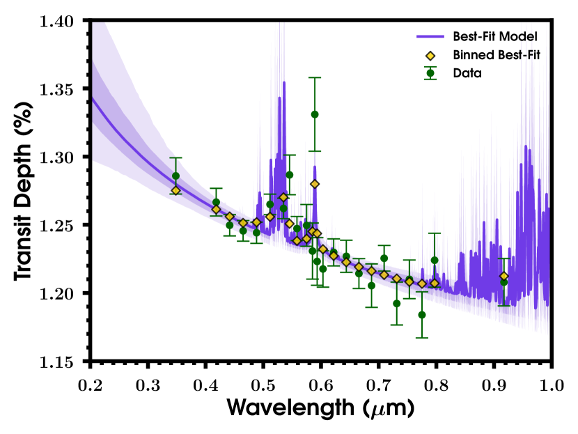
The best-fitting retrieved spectrum is shown in Figure 8. The reduced $\chi^{2}$ for the best-fit model is $\chi^{2}_{\rm red}=1.51$. Comparing the Bayesian evidence for the best-fitting model against a model with no Na absorption, but that is otherwise identical, indicates a detection of Na at $2.9\sigma$ confidence. We retrieve an abundance of $\log X_{\rm Na}=-8.3^{+0.7}_{-0.8}$. The retrieved temperature at the top of our atmosphere ($10^{-5}$ bar) is $2300^{+412}_{-392}$ K, consistent with the equilibrium temperature of the planet, T_eq = 2160 $\pm$ 40 K for an albedo equal to zero (West et al., 2016). We also find marginal evidence for titanium hydride, which may explain the feature around 0.5-0.55$\mu$m. We obtain an upper limit for TiH abundance; $\log X_{\rm TiH}\leq-8.6$. The evidence ratio of the model including only Na and TiH versus the full set of opacities discussed above is 5.3 in favour of the model with fewer chemical species, indicating that other species are not detectable with the present data (Trotta, 2008).

Models incorporating the cloud/haze prescription described above are only slightly preferred to cloud-free models at $1.4\sigma$ confidence. The retrieved value of $\bar{\phi}=0.18^{+0.13}_{-0.11}$ suggests a mostly clear atmosphere. This result indicates that a Rayleigh slope in combination with several atomic or molecular species is the best explanation for the observed transmission spectrum.

Figure 8: Retrieved best-fit transmission spectrum of WASP-76 b. The dark- and light-shaded areas represent 1- and 2-$\sigma$ contours respectively, produced by drawing a sample of 1000 spectra from the retrieved posterior probability distributions. The median best-fit spectrum has been smoothed with a Gaussian filter.

6.3 WASP-76 b in context

A spectral slope caused by scattering from either gas molecules or condensates has been measured in the transmission spectra of many Hot Jupiter exoplanets (e.g., Sing et al., 2011, 2015; Nikolov et al., 2015; Mallonn & Strassmeier, 2016; Chen et al., 2017). Next to absorption features of alkali metals, such a slope is one of very few features in optical transmission spectra that can be used for atmospheric characterization at the current level of commonly achieved measurement precision.

The amplitude of the optical spectral slope of Hot Jupiters has been measured to be typically of order of one to two atmospheric pressure scale heights from the near-UV to the near IR (Sing et al., 2016). No correlation of slope amplitude with planetary temperature and gravity has been found yet (Mallonn & Wakeford, 2017). The amplitude of the slope measured for WASP-76 b turns out to be relatively strong compared to other Hot Jupiters. It is similar in units of pressure scale height to, e.g., HAT-P-32b (Mallonn & Wakeford, 2017), and WASP-6b (Nikolov et al., 2015), but less steep than, e.g., HD 189733b (Sing et al., 2011) and GJ 3470b (Chen et al., 2017; Nascimbeni et al., 2013). Among the ultra-hot planets, a variety of slopes have been found from nearly zero for WASP-19b (Espinoza et al., 2019) and WASP-103b (Lendl et al., 2017) to the sloped spectra of WASP-12b (Sing et al., 2013) and WASP-76 b detected in this work. Thus, ultra-hot Jupiters seem to show a similar diversity in the amplitude of their optical spectral slope as Hot Jupiters of more moderate temperature. We want to note the result of recent studies which showed the slope to be very vulnerable to the effect of systematics, either of instrumental or astrophysical origin (Mackebrandt et al., 2017; Mallonn et al., 2018; Alexoudi et al., 2018). This observational challenge also becomes evident in numerous conflicting published optical slopes of individual targets, e.g. for WASP-19b, WASP-80b, TrES-3b, or GJ 3470b.

The derived transmission spectrum of WASP-76 b shares similarities to the spectrum of WASP-17b (Sing et al., 2016); both show a significant slope and absorption by sodium in low spectral resolution. An atmospheric retrieval of Barstow et al. (2017) on the WASP-17b data of Sing et al. (2016) yielded a Rayleigh-scattering haze layer with a condensate top layer slightly deeper in the atmosphere than for other planets with scattering signature. If similar for WASP-76 b, we would expect to find pronounced water absorption by several scale heights in the near IR for solar composition, only weakly obscured by the relatively deep haze layer. Indeed, the WFC3 transmission spectrum of WASP-76 b, covering wavelengths between 1.1 and 1.6 microns, was analyzed by Tsiaras et al. (2018), who found a significant water feature plus signs of TiO/VO. Contrary to this, Fisher & Heng (2018) used a non-grey cloud model to fit the observed slope, finding a lower water abundance and no detection of TiO/VO. While carrying out our first determination of the wavelength-dependent transit depths, we were not aware of WASP-76’s very bright companion. After comparing the transmission spectrum computed with and without considering the companion, we realized the derived transmission spectrum were offset between each other and had a different slope, making the two set of values inconsistent even at a 3-$\sigma$ level. Both Tsiaras et al. (2018) and Fisher & Heng (2018) do not take into account the presence of the companion and thus neglect the effect that this can have on their derived transmission spectrum. In consequence, we caution the reader against making any conclusion regarding the detection inconsistency of TiO/VO in the atmosphere of WASP-76 b, as this might be caused by the lack of treatment of the stellar companion.

Sodium absorption at the terminator of WASP-76 b was reported by Seidel et al. (2019) using high-resolution transmission spectroscopy. Qualitatively, we confirm the sodium absorption with our approach of low-resolution transmission spectroscopy. However, our value of excess absorption of about 0.15% in a bandwidth of 20 Å compared to the average of the two adjacent bands seems much stronger than the value of Seidel et al. (2019) of 0.37% in the very narrow band of 0.75 Å. To illustrate this difference, we compare the WASP-76 b measurements to HD 189733b. The high-resolution sodium absorption strength of WASP-76 b and HD 189733b is very similar (Seidel et al., 2019; Wyttenbach et al., 2015). However, our low-resolution sodium absorption for WASP-76 b in this work is one order of magnitude stronger than the low-resolution sodium absorption of HD 189733b (Sing et al., 2016). Thus, future follow-up measurements need to verify if the strength of sodium detected in this work is overestimated.

7 Conclusion

In this work, we present the derived primordial composition of the atmosphere of WASP-76 b, covering the near UV to near IR wavelengths. To do so, we analyzed in simultaneous three primary transits obtained with HST/STIS. At first, we observe a large variability in the transmission spectrum, which corresponds to approximately an extension of 3 scale heights, assuming equilibrium temperature. We analyzed some potential causes that could mimic it, including the choice of limb darkening, the impact of stellar activity and the choice of orbital parameters, with special emphasize on the inclination and the semi-major axis. Assuming that the slope is caused by Rayleigh scattering, we derived an atmospheric temperature of 866 $\pm$ 114 K. A $\chi^{2}_{red}$ = 2.17 between data and model, and a clear outlying point around sodium observed in the transmission spectrum, motivated us to carry out an atmospheric retrieval. Through it, we detect sodium at a 2.9$\sigma$ confidence, and retrieve an abundance of $\log X_{\rm Na}=-8.3^{+0.7}_{-0.8}$. The retrieved temperature of 2300${}^{+412}_{-392}$ K is consistent with the equilibrium temperature of the planet. Besides sodium, we obtain some evidence for titanium hydride, however this is still a tentative detection.

Appendix A Posterior distributions for the white light curves

Figure 9: Posterior distributions and correlations between the transit parameters, a/R_S, i, T₀ and R_P/R_S and the coefficients for the linear slope, c₀ and c₁, for the white light curves. Subindex 1, 2 and 3 correspond to each one of the three transits, following the order of Figure 3. Red points correspond to the best-fit parameters and shaded gray to white areas correspond to 1, 2, and 3-$\sigma$ uncertainty regions.

Figure 10: Same as Figure 9, but considering the coefficients for the fourth degree polynomial, namely a₀, a₁, a₂, a₃ and a₄.