VCBART: Bayesian trees for varying coefficients
Abstract
The linear varying coefficient models posits a linear relationship between an outcome and covariates in which the covariate effects are modeled as functions of additional effect modifiers. Despite a long history of study and use in statistics and econometrics, state-of-the-art varying coefficient modeling methods cannot accommodate multivariate effect modifiers without imposing restrictive functional form assumptions or involving computationally intensive hyperparameter tuning. In response, we introduce VCBART, which flexibly estimates the covariate effect in a varying coefficient model using Bayesian Additive Regression Trees. With simple default settings, VCBART outperforms existing varying coefficient methods in terms of covariate effect estimation, uncertainty quantification, and outcome prediction. We illustrate the utility of VCBART with two case studies: one examining how the association between later-life cognition and measures of socioeconomic position vary with respect to age and socio-demographics and another estimating how temporal trends in urban crime vary at the neighborhood level. An R package implementing VCBART is available at https://github.com/skdeshpande91/VCBART.
1 Introduction
1.1 Motivation
The linear varying coefficient model specifies a linear relationship between an outcome and covariates that is allowed to change according to the values of effect modifiers . That is, the model asserts that
| (1) |
where the are functions mapping to and the residual error has mean zero. In this paper, we use Bayesian Additive Regression Trees (BART; Chipman et al., , 2010) to learn the covariate effect functions expressing each with an ensemble of binary regression trees. Our proposed method, which we call VCBART, can produce extremely accurate estimates and well-calibrated uncertainty intervals of evaluations and predictions without imposing rigid parametric assumptions or requiring computationally intensive tuning. VCBART further enjoys strong theoretical guarantees and scales gracefully to large datasets with tens of thousands of observations. The following applications motivate our work.
Socioeconomic position and cognition. A large body of evidence suggests that socioeconomic position (SEP) at different points in the life course is an important determinant of cognitive function in mid-life and older adulthood (Luo and Waite, , 2005; Lyu and Burr, , 2016; Marden et al., , 2017; Greenfield and Moorman, , 2019; Zhang et al., , 2020). A critical open challenge in life course research involves estimating how the associations between cognition and various SEP measures evolve over time and with respect to sociodemographic characteristics. Typically, authors related cognitive outcome to several SEP variables with linear models that included pre-specified interactions between the SEP covariates and characteristics like age, gender, and race. For instance, both Lyu and Burr, (2016) and Marden et al., (2017) modeled an interaction between SEP and age while Aartsen et al., (2019) introduced an additional interaction with age-squared. In doing so, these authors implicitly make strong parametric assumptions about how the associations of interest vary. Unfortunately such functional form assumptions may be inadequate as many of these associations can weaken or level off as people age (see Dupre, , 2007, and references therein).
In Section 5.1, we use VCBART to estimate whether and how the associations between total score on a battery of cognitive assessments and measures of SEP in childhood, early adulthood, and later-life can vary with respect to sociodemographic factors like age, race, and gender. Our dataset comes from the Health and Retirement Study (HRS), which is a nationally representative longitudinal study of US-based adults, and contains total observations of subjects. After adjusting for SEP in early and late adulthood, we found little association between childhood SEP and later-life cognition. Further, after adjusting for SEP in childhood and late adulthood, the association between early adulthood SEP and later-life cognition varied with respect to race and gender but did not vary substantially over time.
Crime in Philadelphia. Over multiple studies of neighborhood-level crime, Balocchi and colleagues have discovered that (i) partially pooling data across adjacent neighborhoods often improves crime forecasts but (ii) ignoring potential spatial discontinuities can yield highly biased forecasts (Balocchi and Jensen, , 2019; Balocchi et al., , 2021, 2023). Spatial discontinuities not only occur along known geographic landmarks (e.g. highways, parks, or rivers) but can also coincide with less visible differences in neighborhood-level demographic and socioeconomic dimensions. Balocchi et al., (2023) fit linear models regressing a transformed crime density onto a time index in each of Philadelphia’s 384 census tracts. Concerned about potential spatial discontinuities in the tract-specific slopes and intercepts, they estimated two partitions of the tracts, one for the slopes and one for the intercepts, in which parameter values were similar within clusters but not across clusters. Working within a Bayesian framework, they identified several high posterior probability partition pairs with an ensemble optimization procedure that greedily searched over the space of pairs of partitions of census tracts.
Although they obtained promising predictive results, their analysis is limited by the assumption that the number of reported crimes within each census tract is monotonic in time. An arguably more realistic model would (i) incorporate higher-order trends to better capture potential non-linearities and (ii) allow the corresponding model coefficients to vary across tracts. That is, a more realistic model would allow for different non-monotonic crime trends in different parts of the city. Unfortunately, extending Balocchi et al., (2023)’s optimization procedure to cover higher-order models is computationally impractical, as it must search over a combinatorially vast product space of partitions. In Section 5.2, we recast their model as a linear varying coefficient model with a single categorical effect modifier recording the census tract. Using VCBART to fit several tract-specific polynomial models, we find that a quadratic model of crime provides a better fit to data than their linear model and other higher-order extensions.
1.2 Our contributions
In both problems, we wish to make minimal assumptions about the functional form of the covariate effects Additionally, at least for the HRS data, we wish to identify which elements of modify the effects of which elements of Further, in both applications, calibrated and coherent uncertainty quantification is imperative. For the HRS data, identifying disparities in the socioeconomic determinants of later-life cognition carry profound public health implications, especially in light of an aging population. And for the crime dataset, accurate assessments of the uncertainty about crime forecasts can inform future public safety policy decisions. Finally, we require a method that can scale to the size of the two motivating datasets, ideally without involving computationally intensive hyperparameter tuning.
Unfortunately, no existing procedure for fitting varying coefficient models meets our desiderata of flexibility, uncertainty quantification, and scalability. To wit, existing state-of-the-art procedures with multivariate modifiers either learn many tuning parameters with leave-one-out cross-validation or rigidly assume that the are additive in the ’s. Moreover, the default implementations of existing procedures do not provide any out-of-sample uncertainty quantification.
We instead approximate each with a sum of regression trees. On synthetic data, our proposed procedure VCBART exhibits superior covariate effect recovery compared to the current state-of-the-art without requiring any hand-tuning or strong structural assumptions. We additionally show that, under mild conditions, the VCBART posterior concentrates at a near-optimal rate, even with correlated residual errors. To the best of our knowledge, our Theorem 1 is the first result demonstrating the theoretical near-optimality of Bayesian treed regression in settings with non-i.i.d. noise.
Here is an outline for the rest of the paper. We briefly review relevant background on VC modeling and BART in Section 2. Then, in Section 3, we introduce VCBART, describe how to perform posterior inference, and state our asymptotic results. In Section 4, we demonstrate VCBART’s excellent covariate effect recovery and predictive capabilities using synthetic data. We apply VCBART to our motivating datasets in Section 5 before outlining several avenues for future work in Section 6.
2 Background
2.1 Varying coefficient models
Since their introduction in Hastie and Tibshirani, (1993), varying coefficient models have been extensively studied and deployed in statistics and econometrics. We give a very brief overview here; see Fan and Zhang, (2008) and Franco-Villoria et al., (2019) for more comprehensive reviews.
When there is only a single modifier (i.e. ), one popular approach to fitting the model in Equation (1) is to express each as a linear combination of pre-specified basis functions (see, e.g. Hoover et al., , 1998; Huang et al., , 2002). Such a decomposition effectively reduces the functional regression problem to a high-dimensional linear regression problem for which numerous frequentist (see, e.g., Wang et al., , 2008; Wang and Xia, , 2009; Wei et al., , 2011) and Bayesian (Bai et al., , 2019) regularization techniques have been proposed. Kernel smoothing is another popular and theoretically supported alternative when (Wu and Chiang, , 2000).
Varying coefficient models are commonly encountered in spatial statistics (see, e.g., Gelfand et al., , 2003; Finley and Banerjee, , 2020). In these settings, there are usually modifiers (space) or modifiers (space and time) and the ’s are typically modeled with Gaussian processes. When the number of observations is large, full Bayesian inference with these models can be computationally demanding, necessitating the use of clever approximations or advanced techniques like distributed computing (Guhaniyogi et al., , 2022). Outside of spatial contexts, to accommodate modifiers, Tibshirani and Friedman, (2020) and Lee et al., (2018) respectively constrained the ’s to be linear and additive functions of the ’s. In contrast, Li and Racine, (2010) proposed a multivariate kernel smoothing estimator that imposes no rigid structural assumptions on the covariate effects. However, the default implementation of their procedure tunes several bandwidth parameters with leave-one-out cross-validation. When or are large, their procedure is computationally prohibitive.
In the last decade, several authors have used regression trees to estimate the covariate effects. Bürgin and Ritschard, (2015), for instance, modeled each with a single regression tree while Wang and Hastie, (2012) and Zhou and Hooker, (2022) both constructed separate ensembles for each using boosting. Unfortunately, existing tree-based procedures require substantial tuning and often do not automatically return any uncertainty estimates.
2.2 Bayesian Additive Regression Trees
Chipman et al., (2010) introduced BART in the context of the standard nonparametric regression problem: given observations from the model they estimated with a sum of piecewise constant step functions, which they represented as binary regression trees. Formally, they computed a posterior distribution over regression tree ensembles, which induces an approximate posterior distribution over regression function evaluations Their regression tree prior, which we adopt and detail in Section 3.1, introduces strong regularization and encourages trees to be “weak learners” in the sense that no one tree explains too much variation in the observed ’s.
The basic BART model has been extended successfully to survival analysis (Sparapani et al., , 2016), multiple imputation (Xu et al., , 2016), log-linear models (Murray, , 2021), semi-continuous responses (Linero et al., , 2020), and causal inference (Hill, , 2011; Hahn et al., , 2020). With conceptually simple modifications, BART can also recover smooth (Linero and Yang, , 2018; Starling et al., , 2020) and monotonic (Starling et al., , 2019; Chipman et al., , 2022) functions. In each setting, BART-based methods often substantially outperform existing procedures in terms of function recovery, prediction, and ease-of-use. Indeed, nearly every BART extension provides default hyperparameters that yield generally excellent performance “off-the-shelf.” Further, recent results in Ročková and Saha, (2019) and Ročková and van der Pas, (2020) demonstrate BART’s theoretical near-optimality under very mild assumptions. See Tan and Roy, (2019) and Hill et al., (2020) for more detailed reviews of BART and its many extensions.
3 The VCBART procedure
Without loss of generality, suppose that we have continuous modifiers, each of which has been re-scaled to lie in the unit interval and categorical or discrete modifiers. For we will assume that the -th categorical modifier can take distinct values contained in some discrete set We further concatenate our modifiers into a vector whose first entries record the values of the continuous modifiers and whose last entries record the values of the categorical modifiers. In other words, each observed modifier vector lies in the product space
Both motivating applications involve repeated measurements over time: in the HRS dataset, we have between four and eight observations per subject and in the crime dataset, we have yearly crime densities in each census tract. For simplicity, we will refer to the observed units (i.e. HRS participants and Philadelphia census tracts) as “subjects.” For each subject we observe triplets of covariates , modifiers , and outcome . For all and we model
| (2) |
We further assume where is a correlation matrix with off-diagonal elements equal to In other words, we assume an exchangeable or compound symmetry correlation structure for each subject’s errors. We assume that the noise vectors ’s are independent across subjects. We do not assume that we observe each subject an equal number of times nor do we assume that the observation times are equally spaced.
The key idea of VCBART is to approximate each function with its own regression tree ensemble. In Section 3.1 we describe the prior over the regression trees and in Section 3.2, we outline strategies for posterior computation and modifier selection.
3.1 Regression tree prior
To set our notation, let be a binary decision tree that consists of a collection of internal nodes and a collection of terminal or leaf nodes. Each internal node of is associated with a decision rule When is a continuous variable, is a half-open interval of the form and when is categorical, is a subset of
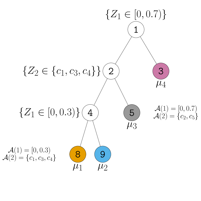
Given and any vector we can imagine tracing a path from the root down the tree by following the decision rules. Specifically, any time the path encounters the rule it proceeds to the left child if Otherwise, it proceeds to the right child. Such decision-following paths continue until they reach a leaf node. It is not difficult to verify that every such path terminates in a single leaf node, implying that induces a partition of into disjoint regions, one for each leaf. By associating each leaf node of with a scalar jump the pair represents a piecewise constant function over where denotes the collections of jumps (see Figure 1 for an example).

For each we introduce an ensemble of regression trees to approximate the function We model each ensemble independently and place independent and identical priors on the individual regression trees within each ensemble. We complete our prior specification with a uniform prior on the autocorrelation and a prior on
We specify the prior for an individual tree in the -th ensemble compositionally with a marginal prior for the decision tree and a conditional prior for the jumps given the tree. Just like in the original BART model, we model the jumps in as a priori independent random variables, where is a positive hyperparameter. Thus, for each the implied marginal prior of is We have found taking to be an effective default choice (see Section S2 of the Supplementary Materials for a hyperparameter sensitivity analysis).
We specify the decision tree prior implicitly by describing how to sample from the prior. First, we draw the overall graphical structure with a branching process that starts from a root node, which is initially considered terminal. Whenever a new terminal node is created at depth , we attach two child nodes to it with probability The quadratic decay ensures that the process terminates at a finite depth.
Given the graphical structure, we draw decision rules at each non-terminal node in two steps. First, we sample the splitting variable index and is the probability of selecting We place a symmetric prior on the vector of splitting probabilities and place a further Beta prior over The implied prior density of is proportional to Although the prior favors sparsity, it has the capacity to include more variables as needed (Linero, , 2018, §3.3). As evidenced by the simulation studies in Linero, (2018), the prior hierarchy on the splitting variable works well in both the sparse setting, when the function depends on only a few variables, and in the non-sparse setting.
Then, conditional on we set to be a random subset of the set of available values at the current non-terminal node (see annotations in Figure 1(a)). When is continuous, is an interval and we set where is drawn uniformly from When is categorical, is a discrete set. How we draw the random subset depends on whether displays network structure like the census tracts in our crime data (see Figure 5(c)). If not, we assign each element of to with probability 0.5. Otherwise, we form by drawing a random network partition. Briefly, we partition the vertices of the subgraph induced by by deleting a random edge from a random spanning tree of the subgraph; see Deshpande, (2023) for details.
3.2 Posterior computation and modifier selection
Conditional regression tree updates. Because the VCBART posterior is analytically intractable, we simulate posterior draws using a Gibbs sampler. Our sampler is a straightforward extension of Chipman et al., (2010)’s basic Bayesian backfitting strategy that sequentially updates each tree conditionally on the other regression trees. Specifically, we update with a Metropolis-Hastings step and transition kernel that randomly grows or prunes the tree. Then, given we draw the jumps from its conditional posterior distribution. Whereas the jumps in the original BART model are conditionally independent, the correlated errors in Equation (2) render the jumps in VCBART conditionally dependent. After updating all trees in the ensemble we perform a conjugate Dirichlet-Multinomial update for the vector of splitting probabilities After sweeping over all ensembles, we update with a Metropolis-Hastings step and update using Roberts and Rosenthal, (2009)’s adaptive Metropolis procedure.
Modifier selection. In our sampler, in order to update the vector of splitting index probabilities we keep track of the number of times each modifier is used in a decision rule in the ensemble Using these counts, we can estimate probability that each is selected at least once in the ensemble used to estimate These selection probabilities are analogous to the posterior inclusion probabilities encountered in Bayesian sparse linear regression. Based on this interpretation, for each ensemble we construct an analog of Barbieri and Berger, (2004)’s median probability model by reporting those modifiers whose selection probability exceeds 0.5.
Before proceeding, we pause to make two remarks about parameter identifiability and our use of a priori independent tree ensembles.
Remark 1 (Identifiability).
For each realization of the modifiers , the vector of covariate function evaluations is identifiable as long as is positive definite (Huang and Shen, , 2004). The individual regression trees, however, are not identified. This is because we can switch the order of the trees without changing the predictions. Nevertheless, in our simulation studies, we did not experience any difficulties recovering the true covariate effects.
Remark 2 (Prior dependence between the ’s).
We introduce a priori independent univariate regression tree ensembles, one for each covariate effect function Despite the prior independence, the observed data likelihood introduces posterior dependence between evaluations Nevertheless, it is natural to wonder how one might introduce prior dependence between the ’s. There are at least two ways. First, one could model the vector-valued with a single ensemble of regression trees with multivariate jumps. Alternatively, one may express each as a linear combination of a common set of basis functions, each of which is modeled as a sum of regression trees. Linero et al., (2020)’s shared forest model uses such an expansion to learn multiple functions simultaneously. In situations where one expects that a modifier may be relevant to some but not all covariate effects, we argue that our separate ensemble approach is preferable. Modeling with a single ensemble of multivariate regression trees or a shared forest essentially assumes that all ’s vary with respect to the same ’s in exactly the same way.
3.3 Posterior contraction of VCBART
With some minor modifications, VCBART enjoys essentially the same favorable theoretical properties as BART — namely, the posterior concentrates at a nearly minimax optimal rate. To facilitate our theoretical analysis of the VCBART posterior, we assume that all modifiers are continuous and have been re-scaled to lie in Like Ročková and Saha, (2019), we modify the decision tree prior so that the probability that the branching process continues growing at depth is for some fixed We further assume that there are truly functions satisfying for each and
| (3) |
where each function is -Hölder continuous with , and . With the additional assumptions (i) that the eigenvalues of are bounded away from zero and infinity and (ii) about the rates at which and diverge as increases, the VCBART posterior concentrates around the true function values at a near-optimal rate as the total number of observations increases. While we defer precise statements of the technical assumptions to Section S1 of the Supplementary Materials, we note here that the assumptions are not restrictive. For instance, we can always re-scale continuous modifiers to the unit interval and, with one-hot encoding, represent categorical modifiers with multiple binary indicators. Further, many commonly used error structures satisfy the required assumptions on the ’s including first-order autoregressive, compound symmetry, and moving averages.
Let be the total number of observations across all subjects, and let and be matrices whose respective -th entries are and Let be the squared empirical norm. If we knew the true smoothness levels the minimax rate for estimating in norm is (Ročková and van der Pas, , 2020). In the absence of this knowledge, Theorem 1 shows that VCBART can estimate the varying coefficients at nearly this rate, sacrificing only a logarithmic factor.
Theorem 1.
Under (3), suppose we endow with a modified VCBART prior, where the splitting probability of each node at depth in a decision tree is given by , for some and the splitting indices are chosen uniformly (i.e. ), and in the half- prior on . Suppose we further endow with the uniform prior, . Assume that assumptions (A1)–(A4) in Section S1 of the Supplementary Materials hold. Then for some constant and ,
| (4) |
in -probability as .
We present the proof of Theorem 1 in Section S1 of the Supplementary Materials.
4 Simulation studies
We performed two simulation studies to understand VCBART’s ability to (i) estimate covariate effect functions and predict future outcomes; (ii) identify which elements of modify the effects of which elements of and (iii) scale to large datasets. We generated data for these experiments from the model in Equation (2) with correlated covariates, potential effect modifiers, and independent within-subject errors. The correlated covariates were drawn from a multivariate normal distribution with mean zero and a covariance matrix with entries The modifiers were drawn uniformly from the interval We used the following covariate effect functions in all experiments
The top row of Figure 2 shows the functions The bottom row of Figure 2 superimposes the VCBART posterior mean and 95% credible intervals for computed using a single dataset from our first experiment, which comprised four observations of subjects for a total of observed ’s. The posterior mean and uncertainty bands were computed after running four independent chains of VCBART for 2,000 iterations, discarding the first 1,000 samples of each as burn-in. We approximated each with an ensemble of trees and set each
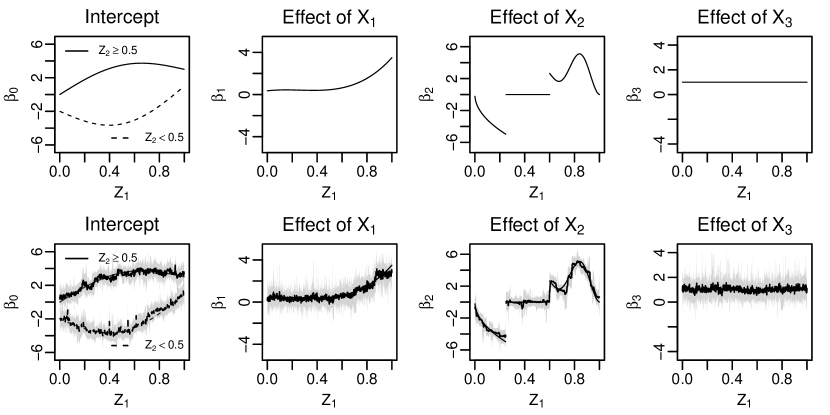
Although the covariate effect functions have very different shapes, VCBART recovered each remarkably well: the posterior means of each closely tracked the shape of the true functions and, for the most part, the true function values were within the shaded pointwise 95% credible intervals. We observed similar behavior for the functions and that depend on multiple effect modifiers (see Figure S1 in the Supplementary Materials). Repeating this experiment twenty five times — that is, fixing the ’s and ’s but simulating the ’s anew — the mean coverage of the 95% posterior credible intervals, averaged across all the ’s, exceeded 99%. Further, averaging across all functions and replications, the mean sensitivity, specificity, precision and F1-score111Letting and FN be the numbers of true positive, true negative, false positive, and false negative identifications in the supports of the ’s, sensitivity is specificity is precision is and the F1 score is for modifier selection with our median probability model were 0.85, 0.99, 0.95, and 0.90, indicating excellent support recovery performance. Sequentially running 4 MCMC chains for 2,000 iterations each took just under one minute on an M1 Mac.
We compared VCBART’s ability to estimate covariate effects out-of-sample to those of the following methods: the standard linear model (lm); Li and Racine, (2010)’s kernel smoothing (KS; implemented in Hayfield and Racine, (2008)’s np package); Bürgin and Ritschard, (2015)’s tree ensemble procedure (TVCM; implemented in Bürgin and Ritschard, (2017)’s vcrpart package); and Zhou and Hooker, (2022)’s boosted tree procedure method (BTVCM; R code available at https://github.com/siriuz42/treeboostVCM). By default, TVCM and KS respectively perform cross-validation to prune the regression trees and to learn kernel bandwidth parameters. The default implementation of BTVCM, on the other hand, does not tune the number of trees or learning rate; in our experiments, we ran the method with 200 trees and with the learning rate used in Zhou and Hooker, (2022)’s experiments.
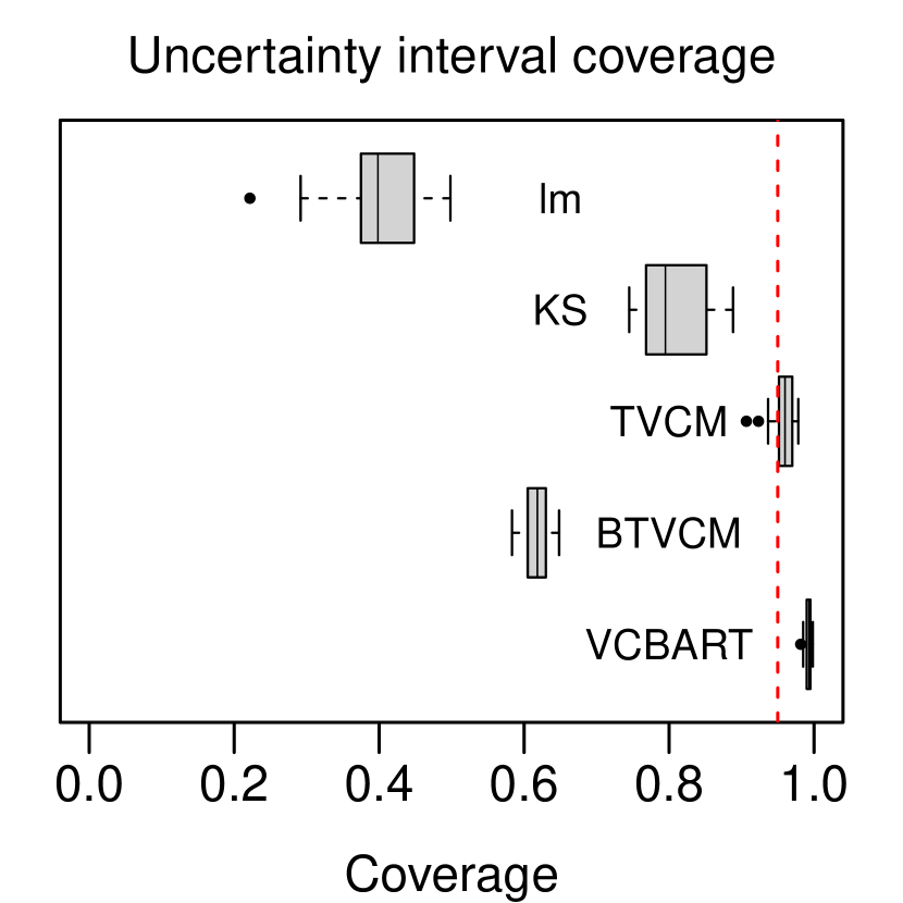
We generated 25 different datasets comprising 250 training subjects and 25 testing subjects, each contributing four observations. That is, we repeatedly trained each method using 1,000 total simulated observations and evaluated performance using an additional 100 observations. As with Figure 2, we ran four chains VCBART for 2,000 iterations, discarding the first 1,000 as “burn-in,” with trees per ensemble and setting each Since the off-the-shelf implementations of KS, TVCM, and BTVCM do not return standard errors of the estimated covariate effects, we formed 95% bootstrap confidence intervals for each using 50 bootstrap resamples. We ran these experiments in a shared high-throughput computing cluster (Center for High Throughput Computing, , 2006). Figures 3(a) and 3(b) compare the out-of-sample mean square error for estimating and uncertainty interval coverages, averaged across all six functions and over all 100 testing set observations. We report function-by-function performance in Section S3.2 of the Supplementary Materials.
In terms of estimating out-of-sample evaluations lm, which assumes that each covariate effect is constant with respect to , performed the worst while VCBART appeared the best. VCBART additionally produced much more accurate predictions and better-calibrated uncertainty intervals than TVCM and BTVCM, the other tree-based varying coefficient procedures. On closer inspection, we further found that the higher coverage of VCBART’s uncertainty intervals was not a by-product of exceedingly wide intervals. In fact, VCBART’s credible intervals for evaluations tended to be shorter than the bootstrapped confidence intervals produced by KS, BTVCM, and TVCM.
Sequentially running four VCBART chains took, on average, about three minutes on our shared cluster. Both lm and BTVCM were faster for these data, with lm running nearly instantaneously and BTVCM producing point estimates in about 90 seconds. That said, both lm and BTVCM produced substantially worse point estimates than VCBART. Although a carefully tuned BTVCM could yield better performance, we expect such tuning would take much longer. We additionally found that obtaining point estimate with TVCM and KS took 1.6 and 9.6 hours, respectively, on average. Sequentially running four chains of VCBART was substantially faster and produced better-calibrated uncertainty intervals than performing 50 bootstrap resamples for BTVCM, TVCM, and KS. In summary, compared to existing methods for fitting varying coefficient models, VCBART was faster and produced more accurate predictions and better-calibrated uncertainty intervals off-the-shelf.
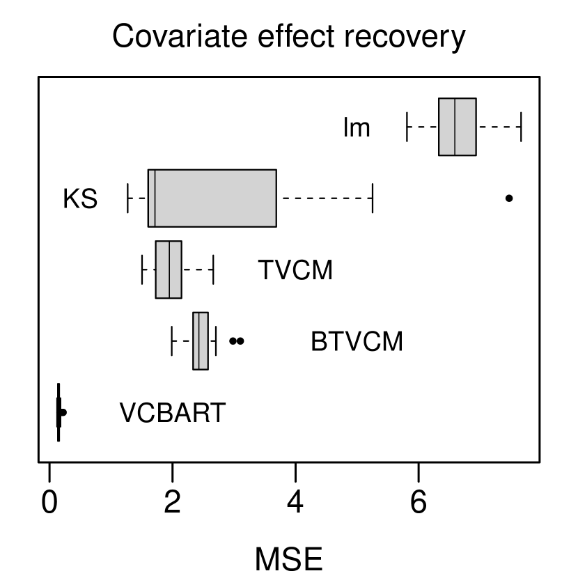
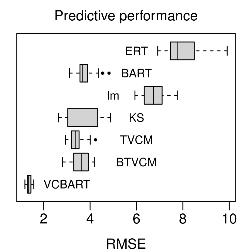
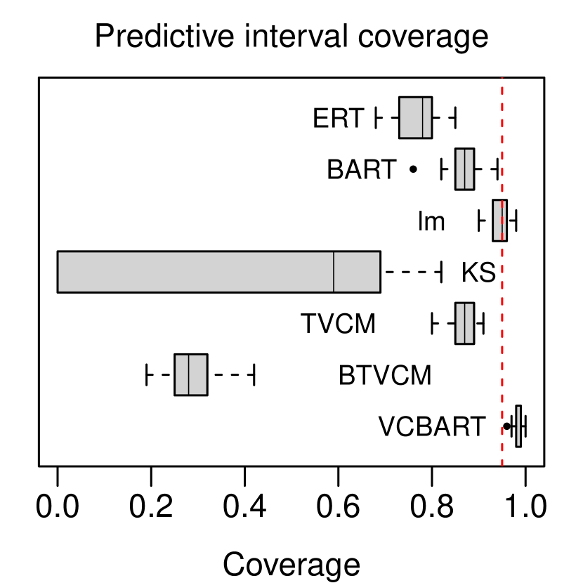
Intuitively, we should expect any method that reliably recovers individual out-of-sample evaluations to yield highly accurate predictions of the outcome And indeed, Figure 3(c) shows that the out-of-sample predictive root mean square error (RMSE) of VCBART and the aforementioned competitors generally track with their estimation error. Figure 3(c) additionally shows that VCBART achieved smaller predictive RMSE than two fully non-parametric methods, BART (implemented in McCulloch et al., (2018)’s BART package) and extremely randomized trees (ERT; implemented in Wright and Ziegler, (2017)’s ranger package). In our experiments, we allowed BART and ERT to use both and to predict Although BART and ERT are facially more flexible than the other competitors, their predictive performance was worse than the correctly-specified varying coefficient methods. Interestingly, however, BART and ERT produced predictive intervals with better coverage than the well-specified BTVCM and KS (Figure 3(d)). That said, VCBART tended to return predictive intervals with better coverage than both BART and ERT.
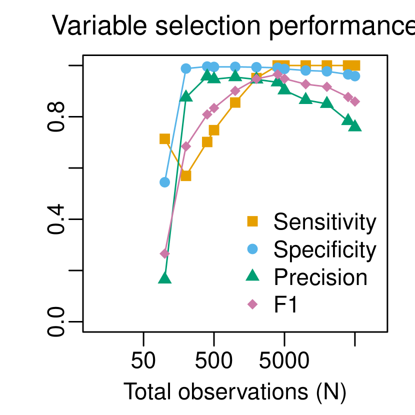
To better understand how well VCBART scales to larger datasets, we conducted a second simulation study. Similar to our first study, we generated 25 synthetic datasets with training subjects and 250 testing subjects, each contributing four observations. We varied between 25 and 12,500, allowing us to see how VCBART performed when trained on as few as 100 and as many as 50,000 total observations. For brevity, we summarize the main findings of that study here and defer more detailed results to Section S3.3 of the Supplementary Materials. Unsurprisingly, as increased, VCBART’s estimation and prediction error decreased and the frequentist coverage of its credible intervals and posterior predictive intervals remained high. In fact, VCBART produced uncertainty intervals with higher-than-nominal frequentist coverage even when fit to as few as total observations. We additionally found that the median probability model’s operating characteristics generally improved a increased. For instance, the F1 score was 0.68 when and exceeded 0.85 for
As each regression tree update involves computing and updating residuals (i.e. a total of operations per iteration), we would expect VCBART to scale linearly in the total number of observations, keeping the total number of MCMC iterations fixed. In our experiments, we observed a strong linear relationship ( between total run time and total number of observations: on an M1 Mac, sequentially running four VCBART chains for 2,000 iterations each took around 55 seconds for observations, 8.5 minutes for observations, and around 48 minutes with observations.
5 Real data examples
5.1 HRS cognition data
To investigate how associations between later-life cognition and socioeconomic position at multiple life stages may vary over time and across sociodemographic characteristics, we analyzed publicly available data from the Health and Retirement Study (HRS). The HRS is a nationally representative longitudinal survey of US adults over the age of 50 and their spouses of any age. Since 1992, the HRS has biennially assessed the economic, health, and social implications of aging through its core survey with response rates greater than 85% in each wave. The HRS is sponsored by the National Institute on Aging (NIA; U01AG009740) and is conducted by the University of Michigan. See Sonnega et al., (2014) for additional details about the HRS.
In each wave, the HRS consistently administered a battery of cognitive tests that include tasks like listening to a series of 10 words and recalling as many possible immediately and several minutes later. The HRS constructed a summary score that ranges from 0 to 35, with higher scores reflecting better cognitive functioning. In our analysis, we use the total cognitive score as our outcome. Our covariate set includes measures of SEP at three distinct stages of life. The first is a composite childhood SEP index, developed and validated by Vable et al., (2017), which is based on the educational attainment and occupation of each subject’s parents and their overall financial well-being in childhood. Higher scores on this index correspond to higher SEP. We additionally included indicators of high school and college completion as proxies of SEP in early adulthood. Finally, as measures of SEP in older adulthood, we used log-income and an indicator of labor force participation. Our modifiers included age in months, gender, race, the U.S. Census division of subject’s birthplace, and an indicator of whether the subject identified as Hispanic.
We restricted our analysis to HRS subjects who (i) had complete covariate, modifier, and outcome data in at least four HRS waves and (ii) were dementia-free in the first wave with complete data. This resulted in analytic sample of subjects who contributed a total of person-years over the study period. In total, we had covariates and potential modifiers. Using the same hyperparameter setting as in Section 4 (i.e. ), we simulated 50 Markov chains of 1,050 iterations. Discarding the first 1,000 samples from each chain as “burn-in,” we obtained a total of 2,500 MCMC samples from the VCBART posterior.
Based on these samples, for each combination of and we computed the posterior probability that the modifier was used in at least one decision rule in the ensemble We then computed the median probability model for each by thresholding these probabilities at 0.5, as described in Section 3.2. The median probability model included gender for all and selected race for all coefficient functions except for the one associated with later-life labor force participation. It additionally identified birthplace as modifying the effects of childhood SEP and high school completion but not the effects of later-life income or labor force participation. Interestingly, our median probability model identified age as a modifier for each covariate except childhood SEP. That is, after adjusting for SEP at later stages of life, our results suggest that differences in later-life cognitive score driven by differences in childhood SEP do not amplify or attenuate over time. In fact, further inspection revealed that the marginal posterior distributions of the estimated partial effect of childhood SEP for subjects in our dataset concentrated within the interval [-0.5, 0.5] and placed roughly equal probability on both positive and negative values. For reference, the sample standard deviation of cognitive scores was about 4 points on a scale ranging rom 0 to 35 points. Our analysis suggests that, after adjusting for SEP in early and older adulthood, childhood SEP has a very small effect, if any, on later-life cognitive scores.
Figure 4 shows the posterior mean and point-wise 95% credible intervals of the predicted intercept and partial effects of childhood SEP and high school completion for two baseline individuals, one Black and one White. Both individuals are females born in the East North Central Census Division of the U.S., which includes the states of Illinois, Indiana, Michigan, Ohio, and Wisconsin. We can interpret the intercept as an average cognitive score for these baseline individuals if they (i) did not complete high school or college and (ii) did not report any earned income or labor force participation in older adulthood.
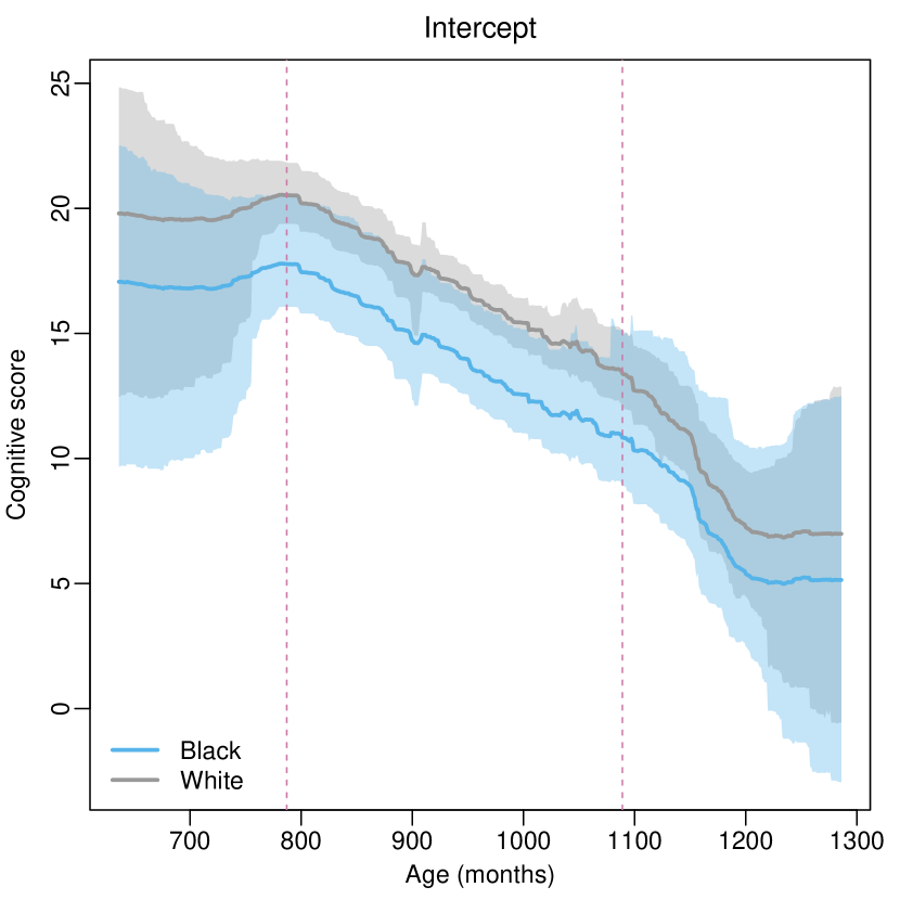
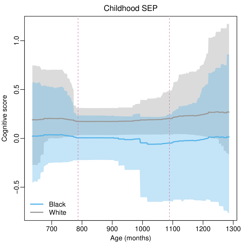
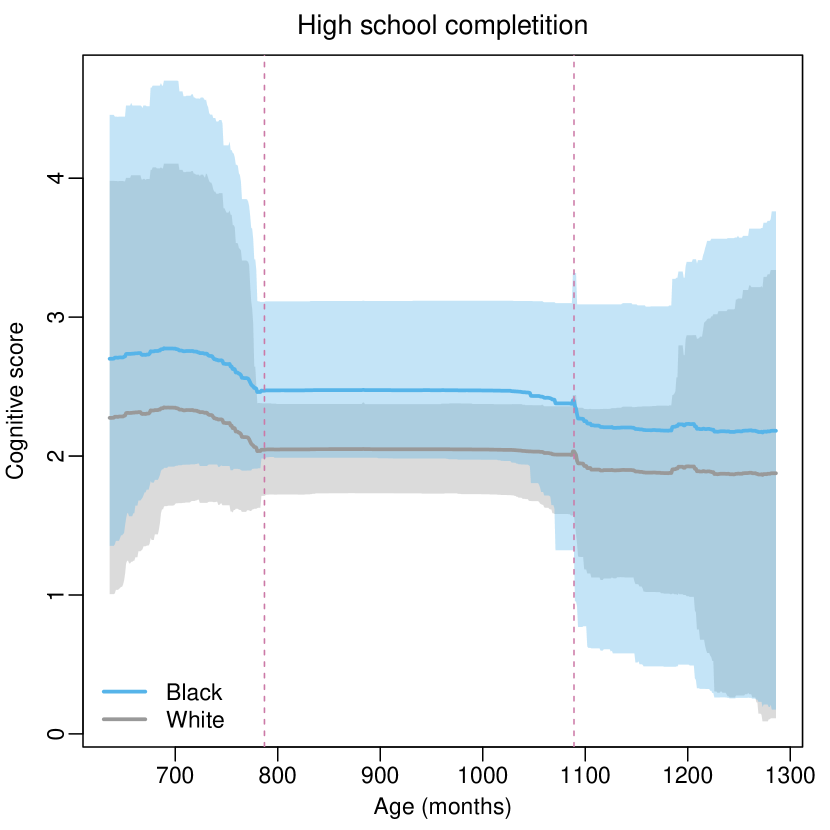
The dashed vertical lines in each panel show the 2.5% and 97.5% quantiles of the distribution of ages in our dataset. Unsurprisingly, there is much more uncertainty about the estimated effects outside of this age range. In Figure 4(a), we observe a steady decline in cognitive scores over time for both baseline individuals as well as a persistent gap between them, with the White individual having slightly higher baseline cognitive scores. As anticipated by our discussion of the median probability model, Figure 4(b) shows that the posterior distributions of the partial effect of childhood SEP for these individuals is concentrated on small positive and negative effect sizes. In sharp contrast, however, we see in Figure 4(c) that high school completion is associated with higher cognitive scores for both baseline individuals. Interestingly, we see that the estimated increase in cognitive score associated with high school completion is slightly higher for the Black baseline individual.
Recall that our median probability model detected temporal variation in the partial effect of high school completion. At least for the two baseline individuals considered in Figure 4(c), that temporal variation appears to manifest mostly in the lower tail of the distribution. Between the ages of 65 and 90 years old, which covers approximately the middle 95% of observed ages in our dataset, the partial effect appears, for all practical purposes, constant over time.
5.2 Philadelphia crime data
The Philadelphia police department releases the latitude and longitude of every reported crime in the city at opendataphilly.org. In each of the census tracts in the city (Figure 5(a)), we computed the yearly crime density, defined as number of crimes per square mile, and applied an inverse hyperbolic sine transformation to counteract the considerable skewness. Let be the transformed crime density in census tract at time with corresponding to 2006 and corresponding to 2021. Balocchi et al., (2023) modeled and computed first-order approximations of each That is, they estimated tract-specific parameters and such that where is a centered and re-scaled version of the time index. Rather than separately estimate each tract’s parameters, they assumed that the intercepts and slopes were spatially clustered. To estimate the latent clusterings, they ran several greedy searches across the space of pairs of census tract partitions.
Despite the reasonably accurate predictions obtained with their first-order approximation, a potential drawback of their analysis is the assumed monotonicity of crime over time. An arguably more realistic model would allow for crime potential increases and decreases within each census tract. Although it is conceptually easy to elaborate their model with higher-order terms, fitting such a model is computationally impractical. Specifically, extending their approach to find an order- polynomial approximation involves searching over the product space of partitions. The combinatorial vastness of this space renders efficient search all but infeasible.
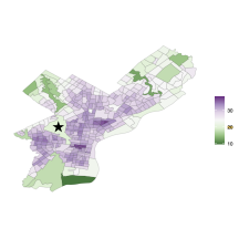
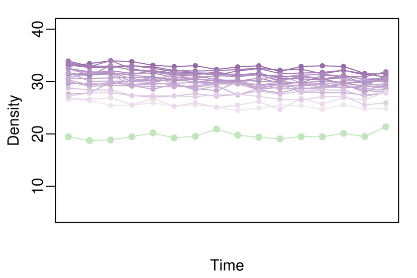
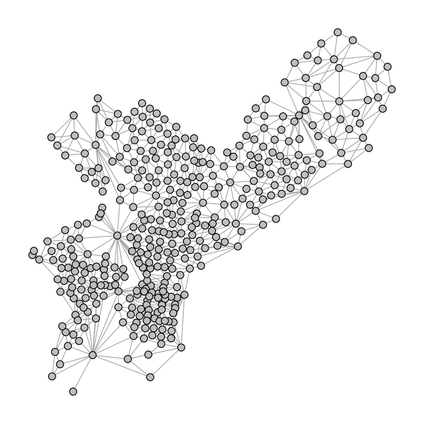
We can instead view their model and higher-order elaborations thereof as varying coefficient models in which the coefficients vary across the vertices of a network determined by census tract adjacency (see Figure 5(c)). Specifically, for a positive integer we can approximate
| (5) |
where we have suggestively expressed the ’s as functions of the census tract label
For a given approximation order fitting the model in Equation (5) is relatively straightforward with VCBART. To encourage spatial smoothness in the ’s, we used a version of the BART prior that is supported on regression trees that recursively partition the network encoded by tract adjacencies (Figure 5(c)) into connected components. Essentially, each individual tree in the ensemble represents a step function taking different values over clusters of spatially contiguous census tracts. See Deshpande, (2023, §3.3) for more details about the prior.
To determine an appropriate order we performed a leave-one-out experiment with the Philadelphia crime data. We specifically considered four approximation orders and two different specifications of the within-tract error structure. The first error structure assumes independence across observations while the second assumes that the errors are equally correlated across time points within each tract (i.e. compound symmetry). For each combination of approximation order and error structure, we fit a VCBART model to all data from all but one census tract and predicted the entire held-out trajectory of transformed crime densities. We ran four MCMC chains for 2,000 iterations each, discarding the first 1,000 iterations as “burn-in.” Table 1 reports the training and testing root mean square error, averaged over all tracts, for each combination of approximation order and error structure.
| RMSE (train) | RMSE (test) | Coverage (train) | Coverage (test) | |
|---|---|---|---|---|
| , ind | 0.61 | 1.99 | 0.97 | 0.78 |
| , ind | 0.55 | 1.97 | 0.98 | 0.79 |
| , ind | 0.52 | 1.93 | 0.98 | 0.80 |
| , ind | 0.50 | 2.02 | 0.98 | 0.81 |
| , cs | 0.67 | 1.95 | 0.98 | 0.79 |
| , cs | 0.60 | 1.83 | 0.98 | 0.79 |
| , cs | 0.57 | 1.91 | 0.98 | 0.79 |
| , cs | 0.55 | 1.93 | 0.98 | 0.78 |
As we might expect, for both error structures, in-sample RMSE decreased with the approximation order However, we found that a quadratic approximation fit with compound symmetry errors yielded the best out-of-sample predictive error. Interestingly, for each we find that the in-sample RMSE is smaller for the model fit with independent errors while the out-of-sample RMSE is smaller for the model with compound symmetry error structure. These finding suggest that ignoring the repeated observation structure of our data tends to overfit the data, regardless of approximation order. Finally, while the average coverage of the marginal 95% predictive intervals exceeded the nominal level in-sample, the out-of-sample average coverages were much lower than nominal.
Further inspection revealed that the out-of-sample predictive interval coverage exceed the nominal 95% level in 235 out of 384 (61%) leave-one-out folds. We suspect that the low average coverage is most likely an artifact of our particular leave-one-out set-up. For the most part, the folds with much lower-than-nominal coverage corresponded to tracts with markedly different crime patterns than their immediate neighbors. As a concrete example, consider the starred tract in Figure 5(a). Arguably no method should produce accurate out-of-sample forecasts when this tract is held out; after all, the crime dynamics from the held-out tract are markedly different than the dynamics in the neighboring tracts observed during training. Consequently, when these tracts were held out in our leave-one-out experiment, the prediction intervals were centered around poor point predictions. In other words, the lower-than-nominal coverage was due more to poor forecasts rather than overconfident predictions.
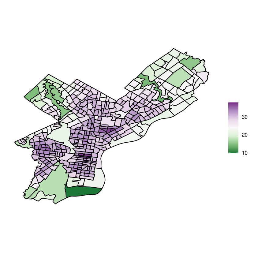
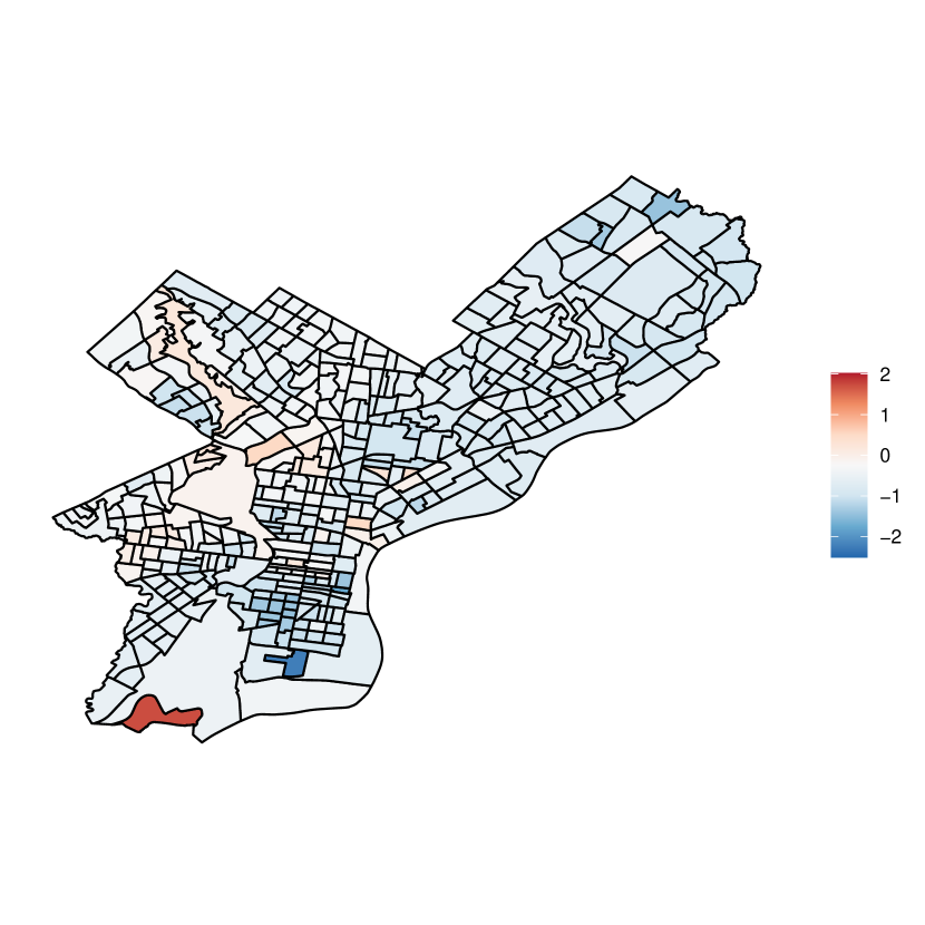
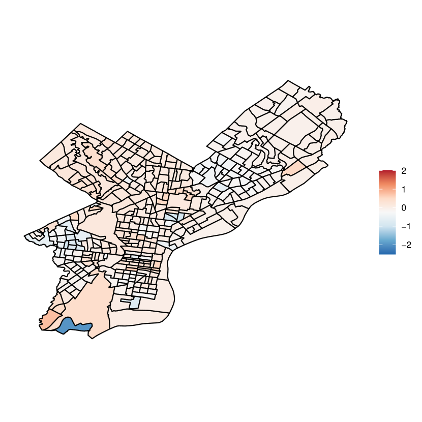
Figure 6 shows the posterior means of the coefficients from the best-fitting model. With some exceptions, we estimated that was negative and was positive in most census tracts. These findings are consistent with the general observations that crime fell city-wide in the early half of the 2010’s before increasing towards the end of the decade and into early-2020. Further, the marginal posterior distributions of the linear coefficient and quadratic coefficient tended to concentrate on small values close to zero. In light of the relatively flat trace plots in Figure 5(b) and for the other census tracts (not shown), such a finding is not entirely unexpected. That said, we found that in around 88% of all census tracts (338 out of 384), the symmetric 95% credible interval for excluded zero and that in about 32% of all tracts (125 out of 384), the credible intervals for both and excluded zero. In other words, our model identified a small non-linear trend in crime with considerably certainty in about a third of all tracts.
6 Discussion
We have introduced VCBART for fitting linear varying coefficient models that retain the interpretability of linear models while displaying predictive accuracy on par with more flexible, blackbox regression models. On simulated data, VCBART displayed covariate effect function recovery and predictive performance superior to existing state-of-the-art VC methods without intensive problem-specific tuning or imposing any structural assumptions about the functions . It moreover returned coherent and generally well-calibrated uncertainty quantifications. Theorem 1 shows that, up to a logarithmic factor, the VCBART posterior concentrates at minimax optimal rate.
In our analysis of the HRS data, we did not explicitly adjust for potential selection biases and confounding. Indeed, it is possible that subjects with higher childhood SEP tended to be better educated and more well-off in later-life. For a more rigorous study of causal effects of SEP on cognitive trajectories, we could use inverse-probability weights as in Marden et al., (2017); indeed, incorporating observation-specific weights to the basic VCBART algorithm is relatively straightforward. Relatedly, the Bayesian causal forest (BCF) models of Hahn et al., (2020) and Woody et al., (2020) are special cases of our more general VCBART model with single covariate. Studying VCBART’s ability to estimate the simultaneous effects of multiple, possibly continuous, treatments under suitable identifying assumptions is an exciting avenue for future development.
In our motivating applications, the number of covariates was relatively small, compared to the number of total observation One can easily imagine, however, settings in which is comparable to or larger than In such settings, running VCBART is challenging as the coefficient functions are no longer identified without further assumptions like sparsity. Under the assumption that only a handful of ’s are truly non-zero functions, we can estimate a sparse varying coefficient model by replacing the normal prior on tree jumps with spike-and-slab priors. Doing so involves introducing an ensemble-specific indicator and, conditionally on the relevant indicator, modeling all jumps in an ensemble as drawn from, for instance, a mean-zero Gaussian distribution with either a very small or very large variance. Such model elaboration inspires a natural Gibbs sampler that iterates between updating these indicators and updating trees within each ensemble. Unfortunately, we would expect this Gibbs sampler to inherit the slow mixing of Gibbs samplers for spike-and-slab regression and for treed regression (Ronen et al., , 2022; Kim and Ročková, , 2023). A potentially more promising computational solution would combine existing fast mode-finding algorithms like EMVS (Ročková and George, , 2014) for sparse regression and the accelerated BART and BCF algorithms (He et al., , 2019; Krantsevich et al., , 2021) for treed regression. Extending these accelerated algorithms to the general varying coefficient model setting is the subject of on-going work.
Finally, throughout this work we have assumed that the sets of covariates and effect modifiers was fixed and known. While domain knowledge and theory often suggest natural choices of effect modifiers, we can readily envision scenarios in which it is not immediately clear whether a particular predictor should enter Equation (1) as a covariate, modifier, or both. In these situations, we recommend setting both and equal to the full set of available predictors.
Acknowledgements
Support for this work was provided by the University of Wisconsin–Madison Office of the Vice Chancellor for Research and Graduate Education with funding from the Wisconsin Alumni Research Foundation (S.K.D.); and National Science Foundation grant DMS-2015528 (R.B.).
References
- Aartsen et al., (2019) Aartsen, M. J., Cheval, B., Sieber, S., Van der Linden, B. W., Gabriel, R., Courvoisier, D. S., Guessous, I., Burton-Jeangros, C., Blane, D., Ihle, A., Kliegel, M., and Cullati, S. (2019). Advantaged socioeconomic conditions in childhood are associated with higher cognitive functioning but strong cognitive decline in older age. Proceedings of the National Academy of Sciences, 116(2):5478–5486.
- Bai et al., (2019) Bai, R., Boland, M. R., and Chen, Y. (2019). Fast algorithms and theory for high-dimensional Bayesian varying coefficient models. arXiv preprint arXiv:1907.06477.
- Balocchi et al., (2023) Balocchi, C., Deshpande, S. K., George, E. I., and Jensen, S. T. (2023). Crime in Philadelphia: Bayesian clustering with particle optimization. Journal of the American Statistical Association, 118(542):818–829.
- Balocchi et al., (2021) Balocchi, C., George, E. I., and Jensen, S. T. (2021). Clustering areal units at multiple levels of resolution to model crime incidence in Philadelphia. arXiv preprint arXiv:2112.02059.
- Balocchi and Jensen, (2019) Balocchi, C. and Jensen, S. T. (2019). Spatial modeling of trends in crime over time in Philadelphia. Annals of Applied Statistics, 13(4):2235–2259.
- Barbieri and Berger, (2004) Barbieri, M. M. and Berger, J. O. (2004). Optimal predictive model selection. Annals of Statistics, 32(3):870–897.
- Bürgin and Ritschard, (2015) Bürgin, R. and Ritschard, G. (2015). Tree-based varying coefficient regression for longitudinal ordinal responses. Computational Statistics and Data Analysis, 86:65–80.
- Bürgin and Ritschard, (2017) Bürgin, R. and Ritschard, G. (2017). Coefficient-wise tree-based varying coefficient regression with vcrpart. Journal of Statistical Software, 80(6):1–33.
- Center for High Throughput Computing, (2006) Center for High Throughput Computing (2006). Center for high throughput computing.
- Chipman et al., (2010) Chipman, H. A., George, E. I., and McCulloch, R. E. (2010). BART: Bayesian Additive Regression Trees. Annals of Applied Statistics, 4(1):266–298.
- Chipman et al., (2022) Chipman, H. A., George, E. I., McCulloch, R. E., and Shively, T. S. (2022). mbart: Multidimensional monotone BART. Bayesian Analysis, 17(2):515–544.
- Deshpande, (2023) Deshpande, S. K. (2023). flexBART: Flexible bayesian regression trees with categorical predictors. arXiv preprint arXiv:2211.04459.
- Dupre, (2007) Dupre, M. E. (2007). Educational differences in age-related patterns of disease: Reconsidering the cumulative disadvantage and age-as-leveler hypotheses. Journal of Health and Social Behavior, 48(1):1–15.
- Eddelbuettel and François, (2011) Eddelbuettel, D. and François, R. (2011). Rcpp: Seamless R and C++ integration. Journal of Statistical Software, 40(8):1 – 18.
- Eddelbuettel and Sanderson, (2014) Eddelbuettel, D. and Sanderson, C. (2014). RcppArmadillo: Accelerating R with high-performance C++ linear algebra. Computational Statistics and Data Analysis, 71:1054 – 1063.
- Fan and Zhang, (2008) Fan, J. and Zhang, W. (2008). Statistical methods with varying coefficient models. Statistics and its Interface, 1:179–195.
- Finley and Banerjee, (2020) Finley, A. O. and Banerjee, S. (2020). Bayesian spatially varying coefficient models in the spBayes R package. Environmental Modelling and Software, 125.
- Franco-Villoria et al., (2019) Franco-Villoria, M., Ventrucci, M., and Rue, H. (2019). A unified view on Bayesian varying coefficient models. Electronic Journal of Statistics, 13(2):5334–5359.
- Gelfand et al., (2003) Gelfand, A. E., Kim, H.-J., Sirmans, C., and Banerjee, S. (2003). Spatial modeling with spatially varying coefficient processes. Journal of the American Statistical Association, 98(462):387–396.
- Ghosal and van der Vaart, (2017) Ghosal, S. and van der Vaart, A. (2017). Fundamentals of Nonparametric Bayesian Infernce. Cambridge University Press.
- Greenfield and Moorman, (2019) Greenfield, E. A. and Moorman, S. M. (2019). Childhood socioeconomic status and later life cognition: Evidence from the Wisconsin Longitudinal Study. Journal of Aging and Health, 31(9):1589–1615.
- Guhaniyogi et al., (2022) Guhaniyogi, R., Li, C., Savitsky, T. D., and Srivastava, S. (2022). Distributed Bayesian varying coefficient modeling using a Gaussian process prior. Journal of Machine Learning Research, 23(84):1–59.
- Hahn et al., (2020) Hahn, P. R., Murray, J. S., and Carvalho, C. M. (2020). Bayesian regression models for causal inference: regularization, confounding, and heterogeneous effects. Bayesian Analysis, 15(3):965–1056.
- Hastie and Tibshirani, (1993) Hastie, T. and Tibshirani, R. (1993). Varying-coefficient models. Journal of the Royal Statistical Society Series B: Statistical Methodology, 55(4):757–796.
- Hayfield and Racine, (2008) Hayfield, T. and Racine, J. S. (2008). Nonparametric econometrics: The np package. Journal of Statistical Software, 27(5).
- He et al., (2019) He, J., Yalov, S., and Hahn, P. R. (2019). XBART: Accelerated Bayesian Additive Regression Trees. In Proceedings of Machine Learning Research. PMLR.
- Hill, (2011) Hill, J. L. (2011). Bayesian nonparametric modeling for causal inference. Journal of Computational and Graphical Statistics, 20(1):217–240.
- Hill et al., (2020) Hill, J. L., Linero, A. R., and Murray, J. S. (2020). Bayesian Additive Regression Trees: A review and look forward. Annual Review of Statistics and its Applications, 7(1):251–278.
- Hoover et al., (1998) Hoover, D. R., Rice, J. A., Wu, C. O., and Yang, L.-P. (1998). Nonparametric smoothing estimates of time-varying coefficient models with longitudinal data. Biometrika, 85(4):809–822.
- Huang and Shen, (2004) Huang, J. Z. and Shen, H. (2004). Functional coefficient regression models for non-linear time series: A polynomial splines approach. Scandinavian Journal of Statistics, 31:515–534.
- Huang et al., (2002) Huang, J. Z., Wu, C. O., and Zhou, L. (2002). Varying-coefficient models and basis function approximations for the analysis of repeated measurements. Biometrika, 89(1):111–128.
- Kim and Ročková, (2023) Kim, J. and Ročková, V. (2023). On mixing rates for Bayesian CART. arXiv preprint arXiv:2306.00126.
- Krantsevich et al., (2021) Krantsevich, N., He, J., and Hahn, P. R. (2021). Stochastic tree ensembles for estimating heterogeneous effects. In Proceedings of the 38th International Conference on Machine Learning. PMLR.
- Lee et al., (2018) Lee, K., Lee, Y. K., Park, B. U., and Yang, S. J. (2018). Time-dynamic varying coefficient models for longitudinal data. Computational Statistics and Data Analysis, 123:50–65.
- Li and Racine, (2010) Li, Q. and Racine, J. S. (2010). Smooth varying-coefficient estimation and inference for qualitative and quantitative data. Econometric Theory, 26(6):1607–1637.
- Linero, (2018) Linero, A. R. (2018). Bayesian regression trees for high-dimensional prediction and variable selection. Journal of the American Statistical Association, 113(522):626–636.
- Linero et al., (2020) Linero, A. R., Sinha, D., and Lipsitz, S. R. (2020). Semiparametric mixed-scale models using shared Bayesian forests. Biometrics, 76(1):131–144.
- Linero and Yang, (2018) Linero, A. R. and Yang, Y. (2018). Bayesian regression tree ensembles that adapt to smoothness and sparsity. Journal of the Royal Statistical Society Series B: Statistical Methodology, 80(5):1087–1110.
- Luo and Waite, (2005) Luo, Y. and Waite, L. J. (2005). The impacts of childhood and adulst SES on physical, mental, and cognitive well-being in later life. The Journals of Gerontology: Series B, 60(2):S93–S101.
- Lyu and Burr, (2016) Lyu, J. and Burr, J. (2016). Socioeconomic status across the life course and cognitive function among older adults: An examination of the latency, pathways, and accumulate hypotheses. Journal of Aging Health, 28(1):40–67.
- Marden et al., (2017) Marden, J., Tchetgen Tchetgen, E. J., Kawachi, I., and Glymour, M. (2017). Contribution of socioeconomic status and 3 life-course periods to late-life memory function and decline: early and late predictors of dementia risk. American Journal of Epidemiology, 186(7):805–814.
- McCulloch et al., (2018) McCulloch, R., Sparapani, R., Gramacy, R., Spanbauer, C., and Pratola, M. (2018). BART: Bayesian Additive Regression Trees. R package version 2.1.
- Murray, (2021) Murray, J. S. (2021). Log-linear Bayesian additive regression trees for categorical and count responses. Journal of the American Statistical Association, 116(534):756–769.
- R Core Team, (2019) R Core Team (2019). R: A language and environment for statistical computing. R Foundation for Statistical Computing, Vienna, Austria.
- Roberts and Rosenthal, (2009) Roberts, G. O. and Rosenthal, J. S. (2009). Examples of adaptive MCMC. Journal of Computational and Graphical Statistics, 18(2):349–367.
- Ronen et al., (2022) Ronen, O., Saarinen, T., Tan, Y. S., Duncan, J., and Yu, B. (2022). A mixing time lower bound for a simplified version of BART. arXiv preprint arXiv:2210.09352v1.
- Ročková and George, (2014) Ročková, V. and George, E. I. (2014). EMVS: The EM approach to Bayesian variable selection. Journal of the American Statistical Association, 109(506):828–846.
- Ročková and Saha, (2019) Ročková, V. and Saha, E. (2019). On theory for BART. In Proceedings of the 22nd International Conference on Artificial Intelligence and Statistics, pages 2839–2848.
- Ročková and van der Pas, (2020) Ročková, V. and van der Pas, S. (2020). Posterior concentration for Bayesian regression trees and forests. Annals of Statistics, 48(4):2108–2131.
- Sonnega et al., (2014) Sonnega, A., Faul, J., Ofstedal, M., Langa, K. M., Phillips, J. W., and Weird, D. R. (2014). Cohort profile: The Health and Retirement Study (HRS). International Journal of Epidemiology, 43(2):576–585.
- Sparapani et al., (2016) Sparapani, R., Logan, B. R., McCulloch, R. E., and Laud, P. W. (2016). Nonparametric survival analysis using Bayesian Additive Regression Trees. Statistics in Medicine, 35(16):2741–2753.
- Starling et al., (2019) Starling, J. E., Aiken, C. E., Murray, J. S., Nakimuli, A., and Scott, J. G. (2019). Monotone function estimation in the presence of extreme data coarsening: Analysis of preeclampsia and birth weight in urban Uganda. arXiv preprint arXiv:1912.06946.
- Starling et al., (2020) Starling, J. E., Murray, J. S., Carvalho, C. M., Bukowski, R., and Scott, J. G. (2020). BART with targeted smoothing: An analysis of patient-specific stillbirth risk. Annals of Applied Statistics, 14(1):28–50.
- Tan and Roy, (2019) Tan, Y. V. and Roy, J. (2019). Bayesian Additive Regression Trees and the General BART model. Statistics in Medicine, 38(25):5048–5069.
- Tibshirani and Friedman, (2020) Tibshirani, R. and Friedman, J. (2020). A pliable lasso. Journal of Computational and Graphical Statistics, 29(1):215–225.
- Vable et al., (2017) Vable, A. M., Gilsanz, P., Nguyen, T. T., Kawachi, I., and Glymour, M. M. (2017). Validation of a theoretically motivated approach to measuring childhood socioeconomic circumstances in the Health and Retirement Study. PLoS ONE, 12(10):e0185898.
- Wang and Xia, (2009) Wang, H. and Xia, Y. (2009). Shrinkage estimation for the varying coefficient model. Journal of the American Statistical Association, 104(486):747–757.
- Wang and Hastie, (2012) Wang, J. C. and Hastie, T. (2012). Boosted varying-coefficient regression models for product demand prediction. Journal of Computational and Graphical Statistics, 23(2):361–382.
- Wang et al., (2008) Wang, L., Li, H., and Huang, J. Z. (2008). Variable selection in nonparametric varying-coefficient models for analysis of repeated measurements. Journal of the American Statistical Association, 103(484):1556–1569.
- Wei et al., (2011) Wei, F., Huang, J., and Li, H. (2011). Variable selection and estimation in high-dimensional varying-coefficient models. Statistica Sinica, 21:1515–1540.
- Woody et al., (2020) Woody, S., Carvalho, C. M., Hahn, P. R., and Murray, J. S. (2020). Estimating heterogeneous effects of continuous exposures using Bayesian tree ensembles: Revising the impact of abortion rates on crime. arXiv preprint arXiv:2007.09845v1.
- Wright and Ziegler, (2017) Wright, M. N. and Ziegler, A. (2017). ranger: A fast implementation of random forests for high dimensional data in C++ and R. Journal of Statistical Software, 77(1):1–17.
- Wu and Chiang, (2000) Wu, C. O. and Chiang, C.-T. (2000). Kernel smoothing on varying coefficient models with longitudinal dependent variable. Statistica Sinica, 10:433–456.
- Xu et al., (2016) Xu, D., Daniels, M. J., and Winterstein, A. G. (2016). Sequential BART for imputation of missing covariates. Biostatistics, 17(3):589–602.
- Zhang et al., (2020) Zhang, Z., Liu, H., and Choi, S.-w. (2020). Early-life socioeconomic status, adolescent cognitive ability, and cognition in late midlife: Evidence from the Wisconsin Longitudinal Study. Social Science & Medicine, 244:112575.
- Zhou and Hooker, (2022) Zhou, Y. and Hooker, G. (2022). Decision tree boosed varying coefficient models. Data Mining and Knowledge Discovery, 36:2237–2271.
Supplementary Materials
S1 Proofs of asymptotic results
S1.1 Notation and Preliminaries
The proof of Theorem 1 is based on the standard prior concentration and testing arguments outlined in Ghosal and van der Vaart, (2017). Roughly speaking, in order to prove optimal posterior concentration, the prior on first needs to be “close” enough to (i.e. the prior needs to assign enough positive probability mass to a neighborhood of ). Second, we need to construct exponentially powerful statistical tests, so that the probabilities of Type I and Type II errors for testing vs. are exponentially decreasing.
Throughout this section, we use the following notation. For two nonnegative sequences and , we write to denote . If , we write or . We use or to denote that for sufficiently large , there exists a constant independent of such that . For a function , . Finally, for a symmetric matrix , we let and denote its minimum and maximum eigenvalues
For two densities and , let and denote the Kullback-Leibler (KL) divergence and KL variation respectively. Denote the Rényi divergence of order 1/2 as . Finally, denote the -covering number for a set with semimetric as the minimum number of -balls of radius needed to cover and denote the -covering number as and the metric entropy as .
To prove near-optimal posterior concentration for VCBART, we need to make the following assumptions. Below, we let and .
-
(A1)
for .
-
(A2)
There exists a constant so that for all .
-
(A3)
and
-
(A4)
The eigenvalues of each within-subject correlation matrix satisfy
and for any
where
Assumption (A1) requires the true ’s to be uniformly bounded. Since the effect modifiers have been rescaled to lie in , this assumption is likely to be satisfied in practice. Assumption (A2) requires that the covariates are uniformly bounded for all . Assumption (A3) allows the number of covariates to diverge to infinity but at a slower rate than . This assumption is needed to ensure that the contraction rate converges to zero as . Assumption (A3) also allows the number of effect modifiers to grow with but at a much slower rate. Assumption (A4) assumes that the within-subject correlation matrices are asymptotically well-behaved in the sense that the eigenvalues for every are bounded away from zero and infinity, and the maximum squared Frobenius norm for the difference between any two correlation matrices of size is bounded above by a function of . Many commonly used correlation structures like first-order autoregressive, compound symmetry, and moving average satisfy this assumption.
S1.2 Proof of Theorem 1
Let , and let denote the vector corresponding to the th subject. Let be the vector of all the ’s. Let and define and . Let denote the probability measure underlying the true model,
| (S1) |
where . Recall that is the total number of observations. For the th observation, the response is distributed as . Let denote the density for and . Analogously, the let be the density for , and let .
The proof of Theorem 1 can be sketched as follows. First we establish the optimal prior concentration for the VCBART prior in Lemma 2 and the optimal posterior contraction with respect to average Rényi divergence of order 1/2 in Lemma 3. This will then imply the optimal posterior contraction in the empirical norm.
Lemma 2.
Under (S1), suppose we endow with the VCBART prior and the autoregressive parameter with the uniform prior, . For the BART priors on the ’s, , suppose that the splitting probability of a node is for some and that the splitting indices are chosen uniformly (i.e. ). For the half- prior on , assume . Assume that Assumptions (A1)-(A4) hold. Then for and some ,
| (S2) |
Proof of Lemma 2.
Our proof follows along the same lines as the proof of Lemma 1 in Bai et al., (2019), with suitable modifications for the fact that we use BART priors on the functionals . Denote . Denote the ordered eigenvalues of by , and let . Noting that the subjects are independent, we have
Define the sets,
Then , and so we can consider separately. Using almost identical arguments as those in the proof of Lemma 1 of Bai et al., (2019),
| (S3) |
for some . Next we focus on bounding from below. Similarly as in the proof of Lemma 1 of Bai et al. (2019), the left-hand side for both inequalities in the set , conditional on , can be bounded above by a constant multiple of . Thus, for some constant , we have as a lower bound for ,
| (S4) |
where , and we used Assumption (A2) about the uniform boundedness of the covariates and an application of the Cauchy-Schwarz inequality in the third line of the display. Since we want to show that , it suffices to show (based on the last line of (S1.2)) that for each function ,
| (S5) |
Note that the lower bound in (S5) holds due to Assumption (A1) that for all , Assumption (A3) that , and the proof of Theorem 7.1 of Ročková and Saha, (2019). Thus, from (S1.2)-(S5), we have that is lower bounded by . Combined with (S3), this yields the desired lower bound in (S2). ∎
Next, we prove posterior contraction of to the truth with respect to average Rényi divergence of order 1/2.
Lemma 3.
Under (S1), suppose we endow with the VCBART prior and the autoregressive parameter with the uniform prior, . For the BART priors on the ’s, , suppose that the splitting probability of a node is for some and that the splitting indices are chosen uniformly (i.e. ). For the half- prior on , assume . Assume that Assumptions (A1)-(A4) hold. Then for and some ,
| (S6) |
in probability as .
Proof of Lemma 3.
This statement will be proven if we can establish that for some ,
| (S7) |
as well as the existence of a sieve such that
| (S8) |
and a test function such that
| (S9) |
We already proved (S7) in Lemma 2. To verify (S8), we consider the sieve,
where for each , is defined as the sieve in the proof of Theorem 7.1 of Ročková and Saha, (2019), i.e. the union of all functions belonging to the class of functions (defined in Ročková and van der Pas, (2020)) that are supported on a valid ensemble (Ročková and van der Pas, , 2020), where each tree in the th ensemble has at most leaves, and is chosen as , for sufficiently large . With this choice of sieve, we have
| (S10) |
Since we assumed that in the half- prior on , is well-defined, and a simple application of the Markov inequality gives for some . Obviously, the second and third terms in (S10) are each equal to , since .
We now focus on bounding the final term in (S10) from above. Let denote the number of terminal leaf notes in the th tree of the th tree ensemble corresponding to the functional . Let , recalling . Noting that all the BART priors have the same number of trees , we have that the second term in (S10) can be bounded above as
| (S11) |
where we used the proof of Theorem 7.1 of Ročková and Saha, (2019) for the third line. By our assumption on the growth rate of in Assumption (A3), we have as for sufficiently large and any . Thus, we have from (S1.2) that the final term on the right-hand side of (S10) is bounded above by for some . Since each of the terms in (S10) can be bounded above by for some constant , we see that (S8) holds.
Now we show the existence of a test function so that (S9) also holds. As in Bai et al., (2019), we first consider the most powerful Neyman-Pearson test for any such that , where and is the density for . If the average Rényi divergence between and is bigger than , then
| (S12) |
By the Cauchy-Schwarz inequality, we have
| (S13) |
and thus, following from the second inequality in (S12) and (S13), we can control the probability of Type II error properly if . Using Assumptions (A2) and (A4) and the same arguments as those in the proof of Lemma 2 in Bai et al., (2019), we have that is bounded above by for densities satisfying
| (S14) |
Combining this with the second inequality in (S12) and (S13) gives
Thus, we see from the first inequality in (S12) and the above inequality that the test satisfying (S9) is obtained as the maximum of all tests described above, for each piece required to cover the sieve. To complete the proof of (S9), we need to show that the metric entropy, , i.e. the logarithm of the maximum number of pieces needed to cover can be bounded above asymptotically by . By Assumption (A2), we have that , and by Assumption (A4), the left-hand side of the second inequality in (S14) is bounded above by on . Thus, for densities satisfying (S14), the metric entropy can be bounded above by
| (S15) |
One can easily verify that the last two terms in (S1.2) are upper bounded by a constant factor of . By modifying the proof of Theorem 7.1 in Ročková and Saha, (2019) appropriately, we have for some and small that the first term in (S1.2) can be upper bounded by
| (S16) |
where is the number of trees in each ensemble . Recalling that is fixed, where , and Assumption (A3) that , we have that each summand in the first term in (S1.2) is upper bounded by , and so (S16) is asymptotically bounded above by . Therefore, from (S1.2)-(S16), we have for densities satisfying (S14),
and so this completes the proof of (S9). Having established (S7)-(S9), it follows that we have posterior contraction with respect to average Rényi divergence, i.e. (S6) holds. ∎
Proof of Theorem 1.
By Lemma 3, in -probability as , where is the Rényi divergence of order 1/2. Under our assumptions and following similar arguments as those in the proof of Lemma 3 in Bai et al., (2019), posterior contraction w.r.t. average Rényi divergence then implies
| (S17) |
where we used Assumption (A1) that for all and Assumption (A2) that the covariates , are uniformly bounded in the third line of the display. In the final line, we used the fact that as . Thus, from (S1.2), the posterior is asymptotically supported on the event for sufficiently large and some large constant . This proves the theorem. ∎
S2 Hyperparameter sensitivity
Recall from the main text, that each ensemble contained trees and we set the prior jump variance This induced a marginal prior on each evaluation Of course, if one has strong prior beliefs about the range of covariate effects, one can set in such a way that the implied marginal prior on places substantial probability on this range. In this section, we consider the sensitivity of VCBART’s covariance effect recovery and predictive capabilities to different choices of Specifically, we replicate the synthetic data experiment from Section 4 of the main text with total observations and vary and for
Figures 7(a) and 7(b) are the analogs of Figures 3a and 3c of the main text, comparing the covariate effect recovery and predictive performance of VCBART with different values of We observed that the coverages of posterior credible intervals for evaluations and predictive intervals for testing outcomes were rather insensitive to both and ; in fact, for each combination of and the intervals all displayed much higher than nominal frequentist coverage. Figure 7(c) shows the F1 score for the median probability model for each combination of and
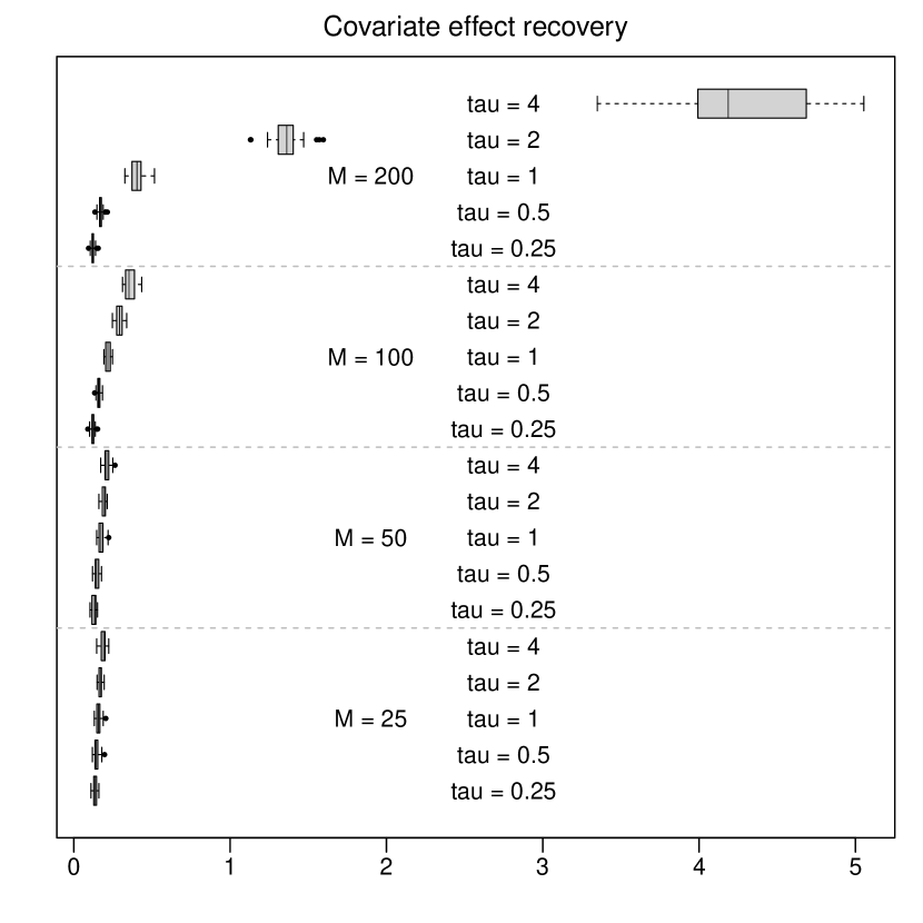
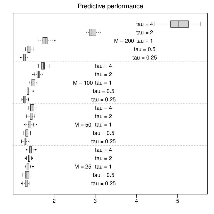
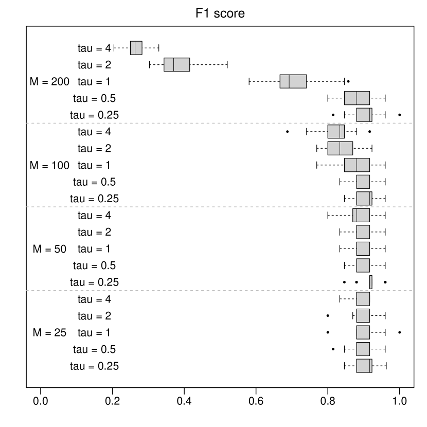
For each we see that as the covariate effect recovery and predictive performance degrades as we increase (resp. decrease) (resp. the amount of regularization). Interestingly, the degree to which performance degrades with increasing also increases with the total number of trees in the ensemble. Put differently, at least for our synthetic data generating process, VCBART’s performance is much more sensitive to when the number of trees is large.
We further observed that the modifier selection performance of VCBART was much worse for than it was for smaller ensemble sizes. On further inspection, we found that the estimated median probability model made too many false positive identifications in the supports of the ’s. That is, the tree ensembles split on too many spurious modifiers We conjecture that the poor performance displayed in the top panel of Figure 7(c) is actually more general. Specifically, the combination of a too large ensemble size and a Dirichlet prior on the vector of splitting probabilities will lead to a proliferation of false positives in the median probability model.
To develop some intuition about this conjecture, suppose that the function has been extremely well-approximated by the first regression trees in an ensemble of size The Gibbs sampling underlying VCBART (and indeed, virtually all BART extensions), updates regression trees based on a partial residual based on the approximation provided by the other trees. Once the sampler reaches the -th tree with , the relevant partial residual will have very little variance. At this point, the tree is being used, essentially, to fit “noise,” with the first trees in the ensemble accounting for virtually all the “signal.” In this situation, spurious decision rules — that is, those based on modifiers that do not drive variation in — are not heavily penalized in the Metropolis-Hastings update. And once a split on a spurious variable has been accepted in a single MCMC iteration, the Dirichlet-Multinomial conjugacy underpinning our decision rule prior, will encourage further splitting on that same variable, leading to a proliferation of false positive identifications. Introducing a dependence on into our decision rule prior might alleviate this behavior. We leave such explorations for future work.
S3 Additional experimental results
S3.1 Implementation details
VCBART is implemented in C++ and interfaces with R (R Core Team, , 2019) through Rcpp (Eddelbuettel and François, , 2011) and RcppArmadillo Eddelbuettel and Sanderson, (2014). Our implementation uses the basic class structures of flexBART (Deshpande, , 2023). We have created an R package VCBART, which is available online at https://github.com/skdeshpande91/VCBART. We performed all of the experiments reported in Sections 4 and 5 of the main text on a high throughput computing cluster (Center for High Throughput Computing, , 2006). All experiments were run in R version 4.1.3 on compute nodes with 10GB of RAM and AMD EPYC 7763 processors.
Where possible, we ran the competing methods in our simulations with package defaults and did not implement any additional tuning procedures. For instance, the default implementation of Zhou and Hooker, (2022)’s boosted tree procedure (referred to as BTVCM in Section 4.1 of the main text) does not automatically perform cross-validation to set the learning rate or number of boosting iterations. Instead, we ran BTVCM for 200 iterations and with a learning rate of 0.5, which are the same settings as the example provided by the authors at https://github.com/siriuz42/treeboostVCM. Similarly the implementation of extremely randomized trees in the ranger package (Wright and Ziegler, , 2017) does not automatically perform cross-validation to select the number of possible splitting variables at each node (i.e. the parameter mtry). In our experiments, we used the package default, setting mtry equal to the square root of the number of inputs.
S3.2 Function-by-function covariate recovery performance
Figure 2 of the main text plotted estimates of and computed after fitting a VCBART model to total observations. Figure S8 plots the posterior means of each against the actual value. With the exception of Figure 8(d), we see that the points fall close to the 45-degree line, indicating that our posterior mean estimates of are close to the actual values used to generate the data. Recall that we generated the data with a constant and with a residual standard deviation of On further inspection, we found that the vast majority of the estimated ’s were within half a standard deviation of the true value So although the VCBART estimates of the constant function were not constant, the estimated values were still quite close to the true function value.


Across the 25 training–testing splits considered in Section 4 of the main text, VCBART produced consistently more accurate estimates of each individual function Figures 3a and 3b in the main text compared the mean square error and uncertainty interval coverage of VCBART and several competitors averaged across all functions and test-set inputs. Figures S9 and S10 are analogs of those two figures that compare the function-by-function mean square and uncertainty interval coverage. We see that VCBART clearly outperforms the other competitors in terms of recovering each function.
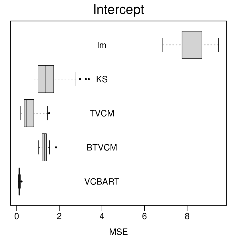

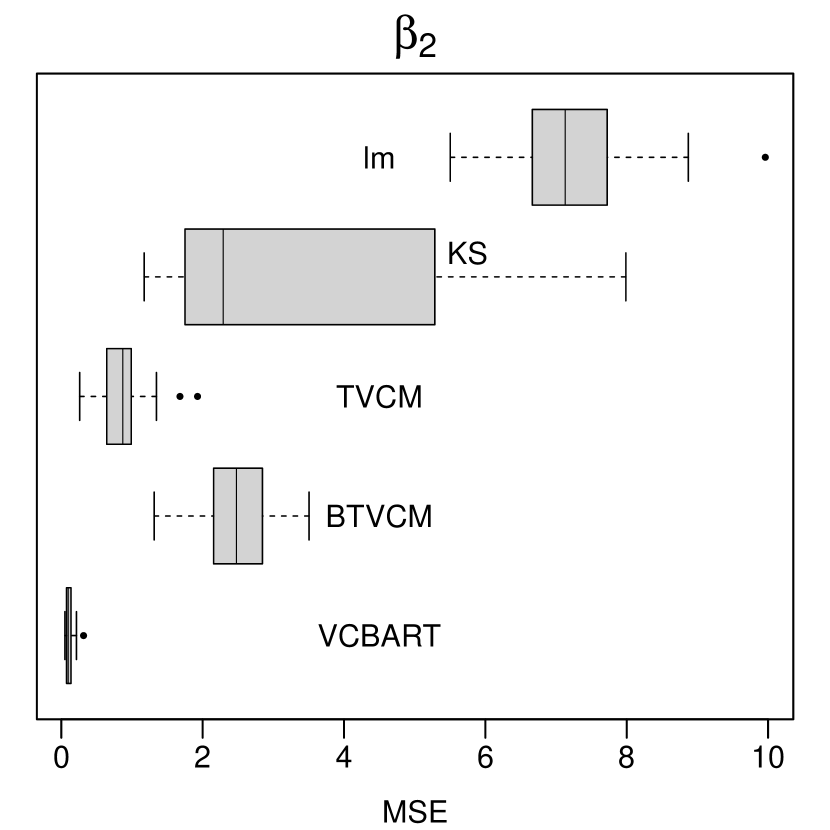

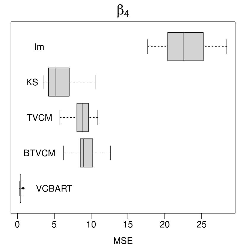
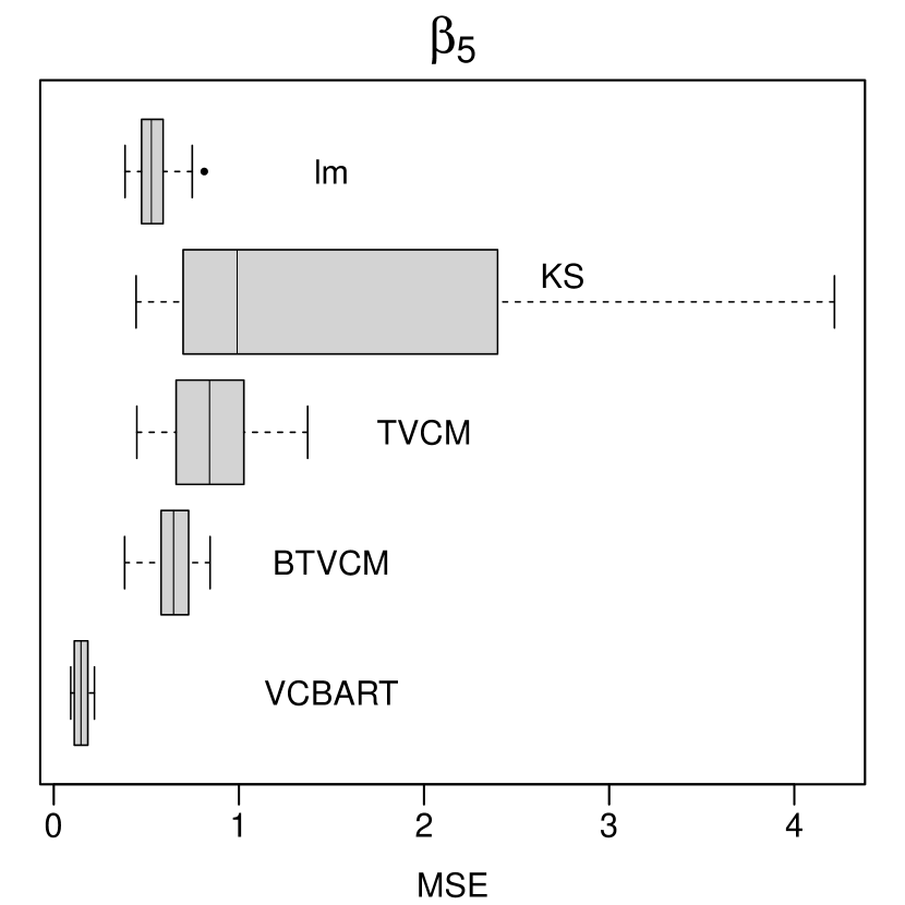
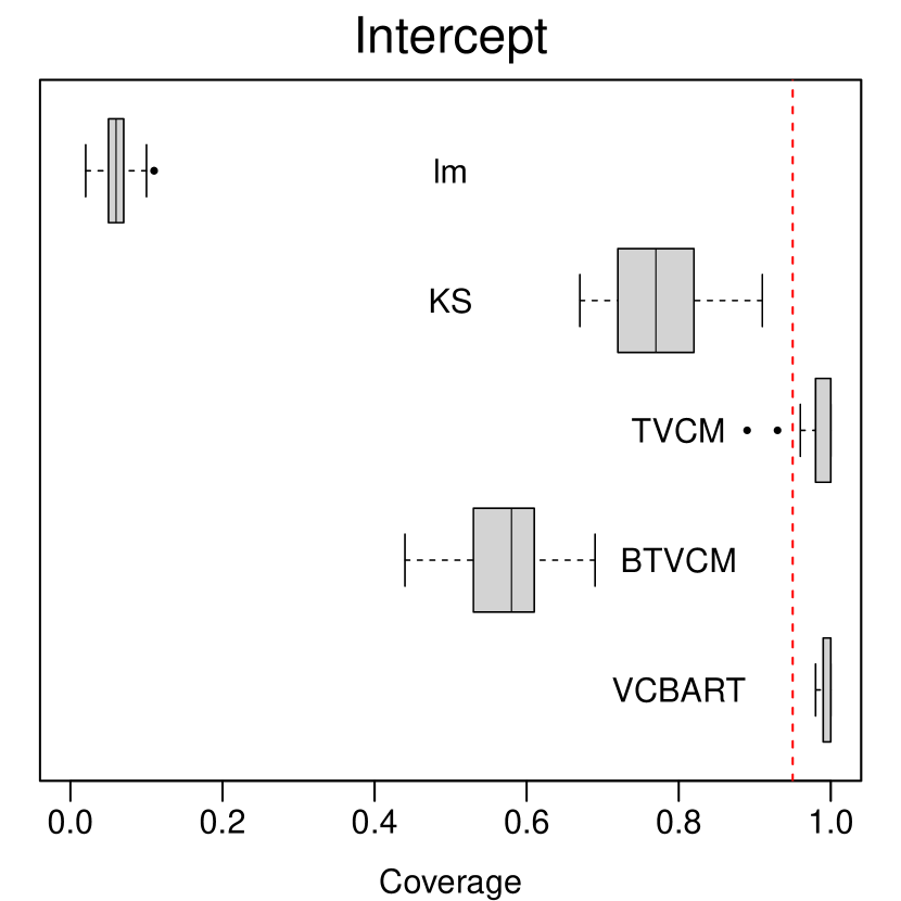
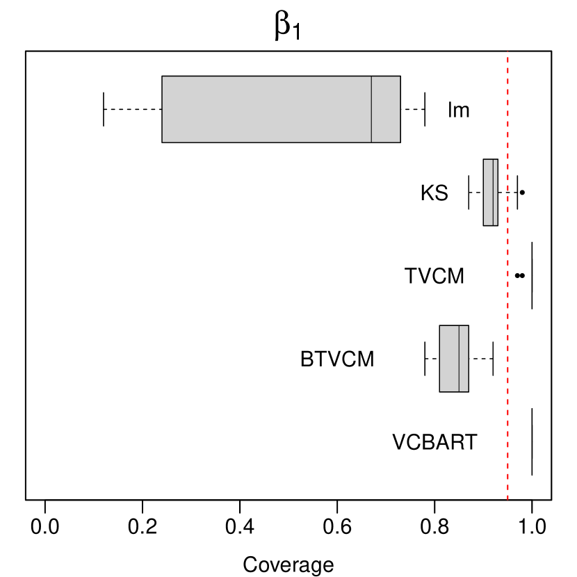
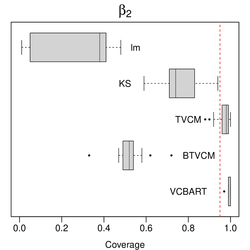

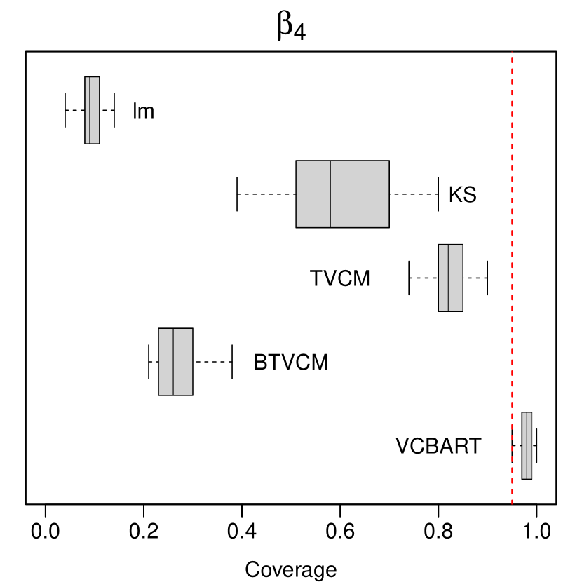
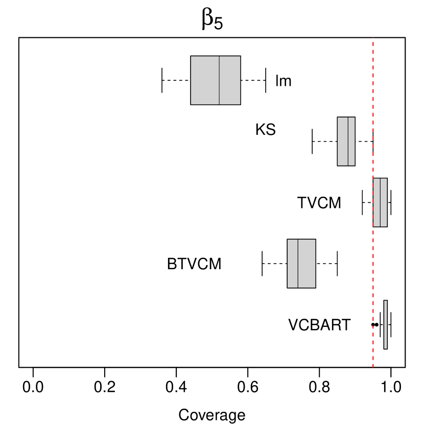
S3.3 Scalability and stability
Recall from Section 4 of the main text that we performed a second synthetic experiment to study VCBART’s ability to scale to larger datasets. Like the main simulation study, we generated data from a varying coefficient model in which each of subject contributed four observations. By varying between 25 and 12,500, we were able to see how VCBART performed when trained on as few as 100 and as many 50,000 total observations. Like our main experiment, we simulated 4 MCMC chains for 2,000 iterations, discarding the first half of each chains as burn-in. Figure S11 plots the covariate effect estimation, uncertainty interval coverage, modifier selection, and runtime as functions of the total number of observations


