Reconstructed Discontinuous Approximation to Stokes Equation in A Sequential Least Squares Formulation

Abstract.

We propose a new least squares finite element method to solve the Stokes problem with two sequential steps. The approximation spaces are constructed by patch reconstruction with one unknown per element. For the first step, we reconstruct an approximation space consisting of piecewise curl-free polynomials with zero trace. By this space, we minimize a least squares functional to obtain the numerical approximations to the gradient of the velocity and the pressure. In the second step, we minimize another least squares functional to give the solution to the velocity in the reconstructed piecewise divergence-free space. We derive error estimates for all unknowns under $L^{2}$ norms and energy norms. Numerical results in two dimensions and three dimensions verify the convergence rates and demonstrate the great flexibility of our method.

Keywords: Stokes problem; Least squares finite element method; Reconstructed discontinuous approximation; Solenoid and irrotational polynomial bases;

MSC2010: 65N30

1. Introduction

The Stokes problem, which models a viscous and incompressible fluid flow, is a linearized version of the full Navier-Stokes equation neglecting the nonlinear convective term. Consequently, the Stokes problem has a large number of applications especially for the time discretization to the Naiver-Stokes problem. Reliable and efficient numerical methods for the Stokes problem have been extensively studied in the references. Among these methods, there were many efforts devoted to develop mixed finite element methods based on the weak formulation of the Stokes problem. A key issue of classical mixed finite element methods is the choice of element types. The pair of finite element spaces are required to satisfy the stability condition, such as the inf-sup condition. We refer the readers to [10, 11, 17] for some examples in classical mixed finite element methods.

The least squares finite element methods for the Stokes problem have been developed in [15, 6, 19, 8, 29, 7, 27, 5]. For these methods, least squares principle together with finite element methods can offer the advantage of circumventing the inf-sup condition arising in mixed methods. Bochev and Gunzburger developed a least squares approach based on rewriting the velocity-vorticity-pressure formulation as a first-order elliptic system [8]. Cai and his coworkers developed the least squares finite element method based on the $L^{2}$ norm residual and $C^{0}$ spaces for the Stokes problem, we refer to [15, 5, 16, 14] for more details. Liu et al. developed a hybrid least squares finite element method based on continuous finite element spaces. This method attempts to combine the advantages of FOSLS and FOSLL* [27]. The works introduced above are based on conforming finite element spaces and such continuous least squares methods are general techniques in numerical methods. We refer to [9] and the references therein for an overview of least squares finite element methods. Based on discontinuous approximation, the discontinuous least squares finite element methods have also been developed for many problems including the Stokes problem, and we refer to [7, 6, 4, 3, 25] for more details.

In this paper, we propose a new least squares finite element method with the reconstructed discontinuous approximation. The novelty is that we propose three specific approximation spaces which allow us to solve the Stokes problem in two sequential steps. The sequential process is motivated from the idea in [26, 15] to define two least-squares-type functionals to approximate unknowns sequentially. The feasibility of this method is based on the new approximation spaces which are obtained by solving local least squares problems on each element. In the first step, we reconstruct an approximation space that consists of piecewise irrotational polynomials with zero trace to approximate the gradient of the velocity. This space is an extension of the space proposed in [23], which will also be used in this step to approximate the pressure. The functions in both approximation spaces may be discontinuous across interior faces and we define a least squares functional with the weak imposition of the continuity across the interior faces to seek numerical solutions in approximation to the gradient and the pressure. In the second step, we reconstruct a piecewise divergence-free polynomial space to approximate the velocity. Here this reconstructed approximation space is also a generalization of the space in [23]. We minimize another least squares functional, together with the numerical gradient obtained in the first step, to solve the numerical solution for the velocity. For the error estimate, we introduce a series of projection operators to derive the convergence rates for all variables with respect to $L^{2}$ norms and energy norms. We prove that the convergence orders under energy norms are all optimal and the $L^{2}$ errors for all variables can only be proved to be sub-optimal. We conduct a series of numerical examples in two dimensions and three dimensions to confirm our theoretical error estimates. In addition, we observe that the $L^{2}$ errors for all unknowns are optimally convergent for approximation spaces of odd orders. Another advantage of our method is the implementation is quite simple. The different types of the reconstruction can be implemented in a uniform way. We present the details to the computer implementation of our method in Appendix A.

The rest of our paper is organized as follow. In Section 2, we give the notations that will be used in this paper. In Section 3, we introduce the reconstruction operators and the corresponding approximation spaces. The approximation properties of spaces are also presented in this section. In Section 4, we define two least squares functionals for sequentially solving the Stokes problem with reconstructed spaces. We also prove the error estimates under $L^{2}$ norms and energy norms. In Section 5, we present a series of numerical results in two dimensions and three dimensions to illustrate the accuracy and the flexibility of our method.

2. Preliminaries

We let $\Omega$ be a convex bounded polygonal (polyhedral) domain in $\mathbb{R}^{d}(d=2,3)$ with the boundary $\partial\Omega$. We denote by $\mathcal{T}_{h}$ a set of polygonal (polyhedral) elements which partition the domain $\Omega$. We denote by $\mathcal{E}_{h}^{i}$ the set of interior faces of $\mathcal{T}_{h}$ and by $\mathcal{E}_{h}^{b}$ the set of the faces that are on the boundary $\partial\Omega$. Let $\mathcal{E}_{h}=\mathcal{E}_{h}^{i}\cup\mathcal{E}_{h}^{b}$ be the set of all $d-1$ dimensional faces. Further, for any element $K\in\mathcal{T}_{h}$ and any face $e\in\mathcal{E}_{h}$ we set $h_{K}$ as the diameter of the element $K$ and $h_{e}$ as the size of the face $e$, and the mesh size is denoted by $h=\max_{K\in\mathcal{T}_{h}}h_{K}$. It is assumed that the partition $\mathcal{T}_{h}$ is shape-regular in the sense of that: there exist

• an integer $N$ that is independent of $h$;

• a number $\sigma>0$ that is independent of $h$;

• a compatible sub-decomposition $\widetilde{\mathcal{T}}_{h}$ into triangles (tetrahedrons);

such that

• every polygon (polyhedron) $K$ in $\mathcal{T}_{h}$ admits a decomposition $\widetilde{\mathcal{T}}_{h|K}$ which has at most $N$ triangles (tetrahedrons);

• for any triangle (tetrahedron) $\widetilde{K}\in\widetilde{\mathcal{T}}_{h}$, the ratio $h_{\widetilde{K}}/\rho_{\widetilde{K}}$ is bounded by $\sigma$ where $h_{\widetilde{K}}$ denotes the diameter of $\widetilde{K}$ and $\rho_{\widetilde{K}}$ denotes the radius of the largest disk (ball) inscribed in $\widetilde{K}$.

The above regularity requirements have several consequences [13, 22]:

• there exists a positive constant $\sigma_{v}$ that is independent of $h$ such that $\sigma_{v}h_{K}\leq h_{e}$ for any element $K\in\mathcal{T}_{h}$ and any face $e\subset\partial K$;

• [trace inequality] there exists a constant $C$ that is independent of $h$ such that

  (2.1) $$\|v\|_{L^{2}(\partial K)}^{2}\leq C\left(h_{K}^{-1}\|v\|_{L^{2}(K)}^{2}+h_{K}\|\nabla v\|_{L^{2}(K)}^{2}\right),\quad\forall v\in H^{1}(K);$$

• [inverse inequality] there exists a constant $C$ that is independent of $h$ such that

  (2.2) $$\|\nabla v\|_{L^{2}(K)}\leq Ch_{K}^{-1}\|v\|_{L^{2}(K)},\quad\forall v\in\mathbb{P}_{k}(K),$$

  where $\mathbb{P}_{k}(\cdot)$ is the polynomial space of degree less than $k$.

For the sub-decomposition $\widetilde{\mathcal{T}}_{h}$, we denote by $\widetilde{\mathcal{E}}_{h}$ the collection of all $d-1$ dimensional faces in $\widetilde{\mathcal{T}}_{h}$, and we decompose $\widetilde{\mathcal{E}}_{h}$ into $\widetilde{\mathcal{E}}_{h}=\widetilde{\mathcal{E}}_{h}^{i}\cup\widetilde{\mathcal{E}}_{h}^{b}$ where $\widetilde{\mathcal{E}}_{h}^{i}$ and $\widetilde{\mathcal{E}}_{h}^{b}$ are the sets of interior faces and boundary faces, respectively. From the regularity assumption, it is clear that $\mathcal{E}_{h}\subset\widetilde{\mathcal{E}}_{h}$, $\mathcal{E}_{h}^{i}\subset\widetilde{\mathcal{E}}_{h}^{i}$ and $\mathcal{E}_{h}^{b}\subset\widetilde{\mathcal{E}}_{h}^{b}$.

Then we introduce the trace operators that are associated with weak formulations. Let $e$ be an interior face shared by two adjacent elements $K^{+}$ and $K^{-}$, and we let $\boldsymbol{\mathrm{n}}^{+}$ and $\boldsymbol{\mathrm{n}}^{-}$ be the unit outward normal on $e$ corresponding to $\partial K^{+}$ and $\partial K^{-}$, respectively. For the scalar-valued function $v$ and the $d$ dimensional vector-valued function $\boldsymbol{q}$ and $d\times d$ dimensional tensor-valued function $\boldsymbol{\tau}$, we define $v^{+}:=v|_{e\subset\partial K^{+}}$, $v^{-}:=v|_{e\subset\partial K^{-}}$, $\boldsymbol{q}^{+}:=\boldsymbol{q}|_{e\subset\partial K^{+}}$, $\boldsymbol{q}^{-}:=\boldsymbol{q}|_{e\subset\partial K^{-}}$, $\boldsymbol{\tau}^{+}:=\boldsymbol{\tau}|_{e\subset\partial K^{+}}$, $\boldsymbol{\tau}^{-}:=\boldsymbol{\tau}|_{e\subset\partial K^{-}}$. The average operator $\{\cdot\}$ on $e$ is defined as

$$\{v\}:=\frac{1}{2}\left(v^{+}+v^{-}\right),\quad\{\boldsymbol{q}\}:=\frac{1}{2}\left(\boldsymbol{q}^{+}+\boldsymbol{q}^{-}\right),\quad\{\boldsymbol{\tau}\}:=\frac{1}{2}\left(\boldsymbol{\tau}^{+}+\boldsymbol{\tau}^{-}\right).$$

The jump operator $[[\cdot]]$ on $e$ is defined as

$$[[v]] :=v^{+}\boldsymbol{\mathrm{n}}^{+}+v^{-}\boldsymbol{\mathrm{n}}^{-},\quad[[\boldsymbol{\mathrm{n}}\times\boldsymbol{q}]]:=\boldsymbol{\mathrm{n}}^{+}\times\boldsymbol{q}^{+}+\boldsymbol{\mathrm{n}}^{-}\times\boldsymbol{q}^{-},$$

$$[[\boldsymbol{\mathrm{n}}\otimes\boldsymbol{q}]] :=\boldsymbol{\mathrm{n}}^{+}\otimes\boldsymbol{q}^{+}+\boldsymbol{\mathrm{n}}^{-}\otimes\boldsymbol{q}^{-},\quad[[\boldsymbol{\mathrm{n}}\otimes\boldsymbol{\tau}]]:=\boldsymbol{\mathrm{n}}^{+}\otimes\boldsymbol{\tau}^{+}+\boldsymbol{\mathrm{n}}^{-}\otimes\boldsymbol{\tau}^{-},$$

where $\otimes$ denotes the tensor product between two vectors. For any tensor $\widehat{\boldsymbol{\tau}}$, if $\mathcal{O}$ is an operator on vector-valued functions, we expend $\mathcal{O}$ to act on $\widehat{\boldsymbol{\tau}}$ columnwise. For example, $\boldsymbol{\mathrm{n}}\otimes\widehat{\boldsymbol{\tau}}$ is defined by

$$\boldsymbol{\mathrm{n}}\otimes\widehat{\boldsymbol{\tau}}:=\boldsymbol{\mathrm{n}}\otimes\left(\widehat{\boldsymbol{\tau}}_{1},\widehat{\boldsymbol{\tau}}_{2},\ldots,\widehat{\boldsymbol{\tau}}_{n}\right)=\left(\boldsymbol{\mathrm{n}}\otimes\widehat{\boldsymbol{\tau}}_{1},\boldsymbol{\mathrm{n}}\otimes\widehat{\boldsymbol{\tau}}_{2},\ldots,\boldsymbol{\mathrm{n}}\otimes\widehat{\boldsymbol{\tau}}_{n}\right)^{T},$$

and $\nabla\cdot\widehat{\boldsymbol{\tau}}$ is defined by

$$\nabla\cdot\widehat{\boldsymbol{\tau}}:=\nabla\cdot\left(\widehat{\boldsymbol{\tau}}_{1},\widehat{\boldsymbol{\tau}}_{2},\ldots,\widehat{\boldsymbol{\tau}}_{n}\right)=\left(\nabla\cdot\widehat{\boldsymbol{\tau}}_{1},\nabla\cdot\widehat{\boldsymbol{\tau}}_{2},\ldots,\nabla\cdot\widehat{\boldsymbol{\tau}}_{n}\right)^{T}.$$

For the boundary face $e$, the trace operators are defined by

$$\{v\}:=v|_{e},\quad\{\boldsymbol{q}\} :=\boldsymbol{q}|_{e},\quad\{\boldsymbol{\tau}\}:=\boldsymbol{\tau}|_{e},$$

$$[[v]]:=v|_{e}\boldsymbol{\mathrm{n}},\quad[[\boldsymbol{\mathrm{n}}\times\boldsymbol{q}]] :=\boldsymbol{\mathrm{n}}\times\boldsymbol{q}|_{e},\quad[[\boldsymbol{\mathrm{n}}\otimes\boldsymbol{q}]]:=\boldsymbol{\mathrm{n}}\otimes\boldsymbol{q}|_{e},\quad[[\boldsymbol{\mathrm{n}}\otimes\boldsymbol{\tau}]]:=\boldsymbol{\mathrm{n}}\otimes\boldsymbol{\tau}|_{e},$$

where $\boldsymbol{\mathrm{n}}$ is the unit outward normal on $e$.

Hereafter, we let $C$ and $C$ with subscripts denote the generic positive constants that may be different from line to line but independent of the mesh size $h$. For a bounded domain $D$, we will use the standard notations and definitions for the Sobolev spaces $L^{2}(D)$, $L^{2}(D)^{d}$, $L^{2}(D)^{d\times d}$, $H^{r}(D)$, $H^{r}(D)^{d}$, $H^{r}(D)^{d\times d}$ with $r$ a positive integer, and we will also use their associated inner products, semi-norms and norms. We define the space of divergence-free functions by

$$\boldsymbol{\mathrm{S}}^{r}(D):=\left\{\boldsymbol{v}\in H^{r}(D)^{d}\ |\ \nabla\cdot\boldsymbol{v}=0\text{ in }D\right\},$$

and we further define the space of tensor-valued functions by

$$\boldsymbol{\mathrm{I}}^{r}(D):=\left\{\boldsymbol{\tau}\in H^{r}(D)^{d\times d}\ |\ \nabla\times\boldsymbol{\tau}=0,\quad\mathrm{tr}\left(\boldsymbol{\tau}\right)=0\text{ in }D\right\},$$

where $\mathrm{tr}\left(\cdot\right)$ denotes the standard trace operator. For the partition $\mathcal{T}_{h}$, we will use the definitions for the broken Sobolev spaces $L^{2}(\mathcal{T}_{h})$, $L^{2}(\mathcal{T}_{h})^{d}$, $L^{2}(\mathcal{T}_{h})^{d\times d}$, $H^{r}(\mathcal{T}_{h})$, $H^{r}(\mathcal{T}_{h})^{d}$, $H^{r}(\mathcal{T}_{h})^{d\times d}$ and their corresponding broken semi-norms and norms. Moreover, for any space $X\in L^{2}(\Omega)$, we let $X/\mathbb{R}$ consist of the functions in $X$ that have zero mean value on $\Omega$,

$$X/\mathbb{R}:=\left\{v\in X\ |\ \int_{\Omega}v\mathrm{d}\boldsymbol{x}=0\right\}.$$

The incompressible Stokes problem we are studying in this paper is formulated as: seeks the velocity fields $\boldsymbol{u}$ and the pressure $p$ such that

(2.3) $$-\nu\Delta\boldsymbol{u}+\nabla p=\boldsymbol{f}, \quad\text{in }\Omega,$$

$$\nabla\cdot\boldsymbol{u}=0, \quad\text{in }\Omega,$$

$$\boldsymbol{u}=\boldsymbol{g}, \quad\text{on }\partial\Omega,$$

where $\boldsymbol{f}$ is a give source term and $\boldsymbol{g}$ is the boundary data and $\nu$ is the reciprocal of the Reynolds number.

As being declared above, we will propose a new least squares finite element method, together with the reconstructed discontinuous approximation, to solve the problem (2.3). We introduce a new inter-mediate variable $\boldsymbol{\mathrm{U}}$ to substitute $\nabla\boldsymbol{u}=(\nabla u^{1},\ldots,\nabla u^{d})$, thus one can reformulate the problem (2.3) into an equivalent first-order system:

(2.4) $$-\nu\nabla\cdot\boldsymbol{\mathrm{U}}+\nabla p=\boldsymbol{f}, \quad\text{in }\Omega,$$

$$\nabla\boldsymbol{u}-\boldsymbol{\mathrm{U}}=\boldsymbol{0}, \quad\text{in }\Omega,$$

$$\nabla\cdot\boldsymbol{u}=0, \quad\text{in }\Omega,$$

$$\boldsymbol{u}=\boldsymbol{g}, \quad\text{on }\partial\Omega.$$

In Section 4, we will go back to the Stokes problem for the details of the sequential least squares method for the first-order system (2.4) with the reconstructed spaces introduced in Section 3.

3. Reconstructed Approximation Space

In this section, we define three types of reconstruction operators that will be used in numerically solving (2.4). The first one is the reconstruction operator which has been used in [24, 22, 25] and the other two operators are extensions from the first one. The reconstruction procedure includes two parts. The first part is to construct the element patch and this part is the same for all reconstruction operators. Now we present the details of the construction to the element patch. We begin by assigning a collocation point in each element. For each element $K$, we specify the barycenter of $K$ as its corresponding collocation point $\boldsymbol{x}_{K}$. Then for each element $K$ we aggregate an element patch $S(K)$ which is a set of elements and consists of $K$ itself and some neighbour elements. Specifically, the element patch $S(K)$ is constructed in a recursive strategy. We first appoint a threshold value $\#S$ to control the cardinality of $S(K)$. We let $S_{0}(K)=\left\{K\right\}$ and construct a sequence of element sets $S_{t}(K)(t\geq 1)$ recursively:

$$S_{t+1}(K)=\bigcup_{\widetilde{K}\in S_{t}(K)}\ \bigcup_{\widehat{K}\in\mathcal{N}(\widetilde{K})}\widehat{K},\quad t=0,1,2,\ldots$$

where $\mathcal{N}(\widetilde{K})$ denotes the set of elements face-neighbouring to $\widetilde{K}$. This recursion ends when the depth $t$ satisfies that the cardinality of $S_{t}(K)$ is greater than $\#S$. We compute the distances between the collocation points of all elements in $S_{t}(K)$ and the point $\boldsymbol{x}_{K}$. We choose the $\#S$ smallest distances and gather the corresponding elements to form the element patch $S(K)$. By this recursive strategy, for any element $K$ the cardinality of $S(K)$ is always $\#S$. After constructing the element patch, for element $K$ we denote by $\mathcal{I}(K)$ the set of the collocation points to the elements in $S(K)$:

$$\mathcal{I}(K):=\left\{\boldsymbol{x}_{\widetilde{K}}\ |\ \forall\widetilde{K}\in S(K)\right\}.$$

Then we will define three reconstruction operators to approximate the functions in $H^{r}(\Omega)$, $\boldsymbol{\mathrm{S}}^{r}(\Omega)$ and $\boldsymbol{\mathrm{I}}^{r}(\Omega)(r\geq 2)$, respectively.

3.1. Reconstruction for Scalar-valued Functions

We denote by ${U}_{h}$ the piecewise constant space associated with $\mathcal{T}_{h}$:

$${U}_{h}:=\left\{v_{h}\in L^{2}(\Omega)\ |\ v_{h}|_{K}\in\mathbb{P}_{0}(K),\quad\forall K\in\mathcal{T}_{h}\right\}.$$

We will define a reconstruction operator $\mathcal{R}^{m}$ from the space $U_{h}$ onto a subspace of the piecewise polynomial space [22]. Given a piecewise constant function $g\in U_{h}$, we will seek a polynomial of degree $m(m\geq 1)$ on every element. For each element $K\in\mathcal{T}_{h}$, we solve the following discrete least squares problem to determine a polynomial $\mathcal{R}_{K}^{m}g$ of degree $m$:

(3.1) $$\mathcal{R}_{K}^{m}g= \mathop{\arg\min}_{q\in\mathbb{P}_{m}(S(K))}\sum_{\boldsymbol{x}\in\mathcal{I}(K)}|q(\boldsymbol{x})-g(\boldsymbol{x})|^{2}$$

$$\text{s.t. }q(\boldsymbol{x}_{K})=g(\boldsymbol{x}_{K}).$$

We follow [22, Assumption B] to make the assumption to ensure the problem (3.1) has a unique solution.

Assumption 1.

For any element $K\in\mathcal{T}_{h}$ and any polynomial $q(\boldsymbol{x})\in\mathbb{P}_{m}(S(K))$, we have that

(3.2) $$p|_{\mathcal{I}(K)}=0\quad\text{implies}\quad p|_{S(K)}=0.$$

The Assumption 3.2 is actually a geometrical assumption which rules out the case that the points in $\mathcal{I}(K)$ are lying on an algebraic curve of degree $m$ and requires the value of $\#S$ shall be greater than the dimension of the polynomial space $\mathbb{P}_{m}(\cdot)$.

Then the reconstruction operator $\mathcal{R}^{m}$ is defined in a piecewise manner:

$$(\mathcal{R}^{m}g)|_{K}=(\mathcal{R}_{K}^{m}g)|_{K},\quad\text{on any element }K\in\mathcal{T}_{h}.$$

We note that the polynomial $\mathcal{R}_{K}^{m}g$ is linearly dependent on $g$. Hence, the operator $\mathcal{R}^{m}$ maps $U_{h}$ onto a subspace of the piecewise polynomial space, which is denoted by $U_{h}^{m}=\mathcal{R}^{m}U_{h}$. For any smooth function $q\in C^{0}(\Omega)$, we define $\widetilde{q}\in U_{h}$ such that

$$\widetilde{q}(\boldsymbol{x}_{K})=q(\boldsymbol{x}_{K}),\quad\forall K\in\mathcal{T}_{h},$$

and we extend the operator $\mathcal{R}^{m}$ to act on the smooth function by defining $\mathcal{R}^{m}q:=\mathcal{R}^{m}\widetilde{q}$.

In addition, we outline a group of basis functions of $U_{h}^{m}$. For any element $K$, we define the characteristic function $w_{K}(\boldsymbol{x})\in U_{h}$ as

$$w_{K}(\boldsymbol{x})=\begin{cases}1,&\boldsymbol{x}\in K,\\ 0,&\text{otherwise},\\ \end{cases}$$

and we denote $\lambda_{K}$ as $\lambda_{K}=\mathcal{R}^{m}w_{K}$.

Lemma 3.1.

The functions $\left\{\lambda_{K}\right\}(\forall K\in\mathcal{T}_{h})$ are linearly independent.

Proof.

For any $\lambda_{K}(\boldsymbol{x})$, the constraint in (3.1) implies that

(3.3) $$\lambda_{K}(\boldsymbol{x}_{\widetilde{K}})=\begin{cases}1,&\widetilde{K}=K,\\ 0,&\widetilde{K}\neq K.\\ \end{cases}$$

We assume that there exist coefficients $\left\{a_{K}\right\}(\forall K\in\mathcal{T}_{h})$ such that

(3.4) $$\sum_{K\in\mathcal{T}_{h}}a_{K}\lambda_{K}(\boldsymbol{x})=0,\quad\forall\boldsymbol{x}\in\Omega.$$

For any element $K$, let $\boldsymbol{x}=\boldsymbol{x}_{K}$ in (3.4) and by (3.3) one see that $a_{K}=0$, which shows that $\left\{\lambda_{K}\right\}$ are linearly independent. This completes the proof. ∎

Clearly, we have that $\text{dim}(\{\lambda_{K}\})=\text{dim}(U_{h})$. The Lemma 3.1 in fact gives that the reconstructed space satisfies $\text{dim}(U_{h}^{m})=\text{dim}(U_{h})$ and $U_{h}^{m}$ is spanned by $\left\{\lambda_{K}\right\}$. Moreover, for the function $g\in U_{h}$ or $g\in C^{0}(\Omega)$, one may write $\mathcal{R}^{m}g$ explicitly:

(3.5) $$\mathcal{R}^{m}g=\sum_{K\in\mathcal{T}_{h}}g(\boldsymbol{x}_{K})\lambda_{K}(\boldsymbol{x}).$$

Then we give the approximation property of the space $U_{h}^{m}$. For any element $K$, we define a constant $\Lambda(m,K)$ as

$$\Lambda(m,K):=\max_{q\in\mathbb{P}_{m}(S(K))}\frac{\max_{\boldsymbol{x}\in S(K)}|q(\boldsymbol{x})|}{\max_{\boldsymbol{x}\in\mathcal{I}(K)}|q(\boldsymbol{x})|}.$$

We let $\Lambda_{m}:=\max_{K\in\mathcal{T}_{h}}(1+\Lambda(m,K)(\#S)^{1/2})$ and in [23, 22] the authors proved that under some mild conditions on element patches, the constant $\Lambda_{m}$ can be bounded uniformly with respect to the partition. These conditions reply on the size of element patches and the authors also proved that if the number $\#S$ is greater than a certain number, the conditions on element patches will be fulfilled, see [22, Lemma 6] and [23, Lemma 3.4]. This certain number is usually too large to be impractical and is not recommended in the implementation. The numerical results demonstrate that our method still has a very good performance even we take the value $\#S$ to be far less than that certain number. In Section 5 we list the values of $\#S$ for different $m$ that are adopted in the numerical tests.

Then we state the following estimate.

Lemma 3.2.

For any element $K$ and any function $g\in C^{0}(\Omega)$, there holds

$$\|g-\mathcal{R}^{m}g\|_{L^{\infty}(K)}\leq\Lambda_{m}\inf_{q\in\mathbb{P}_{m}(S(K))}\|g-q\|_{L^{\infty}(S(K))}.$$

Proof.

We refer to [22, Lemma 3] for the proof. ∎

From Lemma 3.2, it is easy to derive the following approximation properties.

Theorem 3.1.

For any element $K$, there exist constants $C$ such that

(3.6) $$\|g-\mathcal{R}^{m}g\|_{H^{q}(K)} \leq C\Lambda_{m}h_{K}^{m+1-q}\|g\|_{H^{m+1}(S(K))},\quad q=0,1,$$

$$\|\nabla^{q}(g-\mathcal{R}^{m}g)\|_{L^{2}(\partial K)} \leq C\Lambda_{m}h_{K}^{m+1-q-1/2}\|g\|_{H^{m+1}(S(K))},\quad q=0,1,$$

for any $g\in H^{m+1}(\Omega)$.

Proof.

We refer to [22, Lemma 4] for the proof. ∎

3.2. Reconstruction for Vector-valued Functions

Here we consider to extend the reconstruction process for vector-valued functions. Precisely, we will introduce a reconstruction operator for functions in the space $\boldsymbol{\mathrm{S}}^{m+1}(\Omega)$. We also start from the piecewise constant space $(U_{h})^{d}$. Given a function $\boldsymbol{g}\in(U_{h})^{d}$ and for any element $K\in\mathcal{T}_{h}$, we solve a polynomial $\widetilde{\mathcal{R}}_{K}^{m}\boldsymbol{g}$ of degree $m$ on $S(K$) by the following discrete least squares problem:

(3.7) $$\widetilde{\mathcal{R}}_{K}^{m}\boldsymbol{g}=\mathop{\arg\min}_{\boldsymbol{q}\in\mathbb{P}_{m}(S(K))^{d}} \sum_{\boldsymbol{x}\in\mathcal{I}(K)}\|\boldsymbol{q}(\boldsymbol{x})-\boldsymbol{g}(\boldsymbol{x})\|_{l^{d}}^{2},$$

s.t. $$\begin{cases}\boldsymbol{q}(\boldsymbol{x}_{K})=\boldsymbol{g}(\boldsymbol{x}_{K}),\\ \nabla\cdot\boldsymbol{q}=0,\\ \end{cases}$$

where

$$\|\boldsymbol{v}\|_{l^{d}}^{2}:=v_{1}^{2}+\ldots+v_{d}^{2},\quad\forall\boldsymbol{v}=(v_{1},\ldots,v_{d})^{T}\in\mathbb{R}^{d}.$$

Based on Assumption 3.2, it is trivial to check the uniqueness and the existence of the solution to the problem (3.7). Then the reconstruction operator $\widetilde{\mathcal{R}}^{m}$ is piecewise defined as

$$(\widetilde{\mathcal{R}}^{m}\boldsymbol{g})|_{K}=(\widetilde{\mathcal{R}}_{K}^{m}\boldsymbol{g})|_{K},\quad\text{on any element }K\in\mathcal{T}_{h}.$$

It should be noted that $\widetilde{\mathcal{R}}^{m}_{K}\boldsymbol{g}$ still has a linear dependence on $\boldsymbol{g}$. Therefore, we can know that the operator $\widetilde{\mathcal{R}}^{m}$ maps the space $(U_{h})^{d}$ into the piecewise divergence-free polynomial space of degree $m$, and we denote by $\boldsymbol{\mathrm{S}}_{h}^{m}=\widetilde{\mathcal{R}}^{m}(U_{h})^{d}$. We also extend the operator $\widetilde{\mathcal{R}}^{m}$ to act on the smooth function as the operator $\mathcal{R}^{m}$. For the function $\boldsymbol{g}(\boldsymbol{x})\in C^{0}(\Omega)^{d}$, we define a piecewise constant function $\widetilde{\boldsymbol{g}}(\boldsymbol{x})\in(U_{h})^{d}$ such that

$$\widetilde{\boldsymbol{g}}(\boldsymbol{x}_{K})=\boldsymbol{g}(\boldsymbol{x}_{K}),\quad\forall K\in\mathcal{T}_{h},$$

and we define $\widetilde{\mathcal{R}}^{m}\boldsymbol{g}:=\widetilde{\mathcal{R}}^{m}\widetilde{\boldsymbol{g}}$. We also present a group of basis functions to the space $\boldsymbol{\mathrm{S}}_{h}^{m}$. For any element $K$, we define an indicator function $\widetilde{\boldsymbol{w}}_{K}^{i}(\boldsymbol{x})\in(U_{h})^{d}$, which reads

$$\widetilde{\boldsymbol{w}}_{K}^{i}(\boldsymbol{x})=\begin{cases}\boldsymbol{e}_{i},&\boldsymbol{x}\in K,\\ 0,&\text{otherwise},\\ \end{cases}$$

where $\boldsymbol{e}_{i}$ is a $d\times 1$ unit vector whose $i$-th entry is $1$. Then we define $\widetilde{\boldsymbol{\lambda}}_{K}^{i}$ as $\widetilde{\boldsymbol{\lambda}}_{K}^{i}=\widetilde{\mathcal{R}}^{m}_{K}\widetilde{\boldsymbol{w}}_{K}^{i}$ and we have the following lemma.

Lemma 3.3.

The functions $\left\{\boldsymbol{\lambda}_{K}^{i}\right\}(\forall K\in\mathcal{T}_{h},1\leq i\leq d)$ are linearly independent.

Proof.

The proof results from the constraint in (3.7) and is similar to the proof of Lemma 3.1. ∎

Analogously, we conclude that the space $\boldsymbol{\mathrm{S}}_{h}^{m}$ is spanned by $\{\widetilde{\boldsymbol{\lambda}}_{K}^{i}\}$ and for the function $\boldsymbol{g}=(g^{1},\ldots,g^{d})\in(U_{h})^{d}$ or $\boldsymbol{g}=(g^{1},\ldots,g^{d})\in C^{0}(\Omega)^{d}$, we can write $\widetilde{\mathcal{R}}^{m}\boldsymbol{g}$ as

$$\widetilde{\mathcal{R}}^{m}\boldsymbol{g}=\sum_{K\in\mathcal{T}_{h}}\sum_{i=1}^{d}g^{i}(\boldsymbol{x}_{K})\widetilde{\boldsymbol{\lambda}}_{K}^{i}(\boldsymbol{x}).$$

Further, we give the approximation property of the operator $\widetilde{\mathcal{R}}^{m}$.

Lemma 3.4.

For any element $K$ and any function $\boldsymbol{g}\in C^{0}(\Omega)^{d}$, there holds

(3.8) $$\|\boldsymbol{g}-\widetilde{\mathcal{R}}^{m}\boldsymbol{g}\|_{L^{\infty}(K)}\leq\sqrt{d}\Lambda_{m}\inf_{\boldsymbol{q}\in\mathbb{P}_{m}(S(K))^{d}\cap\boldsymbol{\mathrm{S}}^{0}(S(K))}\|\boldsymbol{g}-\boldsymbol{q}\|_{L^{\infty}(S(K))}.$$

Proof.

For any divergence-free polynomial $\boldsymbol{q}\in\mathbb{P}_{m}(S(K))^{d}\cap\boldsymbol{\mathrm{S}}^{0}(S(K))$, we clearly have that $\widetilde{\mathcal{R}}^{m}_{K}\boldsymbol{q}=\boldsymbol{q}$ from the definition of the least squares problem (3.7). We deduce that

$$\|\boldsymbol{g}-\widetilde{\mathcal{R}}^{m}\boldsymbol{g}\|_{L^{\infty}(K)} \leq\|\boldsymbol{g}-\boldsymbol{q}\|_{L^{\infty}(K)}+\|\widetilde{\mathcal{R}}^{m}(\boldsymbol{q}-\boldsymbol{g})\|_{L^{\infty}(K)}$$

$$\leq\|\boldsymbol{g}-\boldsymbol{q}\|_{L^{\infty}(K)}+\Lambda(m,K)\max_{\boldsymbol{x}\in\mathcal{I}(K)}|\widetilde{\mathcal{R}}^{m}(\boldsymbol{q}-\boldsymbol{g})|$$

$$\leq\|\boldsymbol{g}-\boldsymbol{q}\|_{L^{\infty}(K)}+\Lambda(m,K)\sqrt{d\#S}\max_{\boldsymbol{x}\in\mathcal{I}(K)}|\boldsymbol{q}-\boldsymbol{g}|$$

$$\leq\sqrt{d}\left(1+\Lambda(m,K)\sqrt{\#S}\right)\|\boldsymbol{g}-\boldsymbol{q}\|_{L^{\infty}(S(K))},$$

which gives us the estimate (3.8) and completes the proof. ∎

Theorem 3.2.

For any element $K$, there exist constants $C$ such that

(3.9) $$\|\boldsymbol{g}-\widetilde{\mathcal{R}}^{m}\boldsymbol{g}\|_{H^{q}(K)} \leq C\Lambda_{m}h_{K}^{m+1-q}\|\boldsymbol{g}\|_{H^{m+1}(S(K))},\quad q=0,1,$$

$$\|\nabla^{q}(\boldsymbol{g}-\widetilde{\mathcal{R}}^{m}\boldsymbol{g})\|_{L^{2}(\partial K)} \leq C\Lambda_{m}h_{K}^{m+1-q-1/2}\|\boldsymbol{g}\|_{H^{m+1}(S(K))},\quad q=0,1,$$

for any $\boldsymbol{g}\in\boldsymbol{\mathrm{S}}^{m+1}(\Omega)$.

Proof.

By [2, Theorem 4.1] and [22, Assumption A], there exists an approximation polynomial $\widetilde{\boldsymbol{q}}\in\mathbb{P}_{m}(S(K))^{d}\cap\boldsymbol{\mathrm{S}}^{0}(S(K))$ such that

$$\|\boldsymbol{g}-\widetilde{\boldsymbol{q}}\|_{L^{\infty}(S(K))}\leq Ch_{K}^{m+1-d/2}\|\boldsymbol{g}\|_{H^{m+1}(S(K))}.$$

By Lemma 3.8, we obtain that

$$\|\boldsymbol{g}-\widetilde{\mathcal{R}}^{m}\boldsymbol{g}\|_{L^{2}(K)} \leq Ch_{K}^{d/2}\|\boldsymbol{g}-\widetilde{\mathcal{R}}^{m}\boldsymbol{g}\|_{L^{\infty}(K)}\leq Ch_{K}^{d/2}\Lambda_{m}\|\boldsymbol{g}-\widetilde{\boldsymbol{q}}\|_{L^{\infty}(S(K))}$$

$$\leq C\Lambda_{m}h_{K}^{m+1}\|\boldsymbol{g}\|_{H^{m+1}(S(K))},$$

and together with the inverse inequality M2, we have that

$$\|\boldsymbol{g}-\widetilde{\mathcal{R}}^{m}\boldsymbol{g}\|_{H^{1}(K)} \leq\|\boldsymbol{g}-\widetilde{\boldsymbol{q}}\|_{H^{1}(K)}+\|\widetilde{\boldsymbol{q}}-\widetilde{\mathcal{R}}^{m}\boldsymbol{g}\|_{H^{1}(K)}\leq\|\boldsymbol{g}-\widetilde{\boldsymbol{q}}\|_{H^{1}(K)}+Ch_{K}^{-1}\|\widetilde{\boldsymbol{q}}-\widetilde{\mathcal{R}}^{m}\boldsymbol{g}\|_{L^{2}(K)}$$

$$\leq C\Lambda_{m}h_{K}^{m+1}\|\boldsymbol{g}\|_{H^{m+1}(S(K))}.$$

Applying the trace inequality M2 gives the trace estimate in (3.9), which completes the proof. ∎

3.3. Reconstruction for Tensor-valued Functions

In this subsection, we consider the reconstruction for the tensor-valued functions in the space $\boldsymbol{\mathrm{I}}^{m+1}(\Omega)$. Again, we start from a piecewise constant space. Since the functions in $\boldsymbol{\mathrm{I}}^{m+1}(\Omega)$ have zero trace, we define the space $\boldsymbol{\mathrm{U}}_{h}$ consisting of piecewise constant functions with zero trace, which reads

$$\boldsymbol{\mathrm{U}}_{h}:=\left\{\boldsymbol{v}_{h}\in(U_{h})^{d\times d}\ |\ \mathrm{tr}\left(\boldsymbol{v}_{h}\right)=0\right\}.$$

For the function $\boldsymbol{g}\in\boldsymbol{\mathrm{U}}_{h}$, we will seek a polynomial $\widehat{\mathcal{R}}_{K}^{m}\boldsymbol{g}$ of degree $m$ on $S(K)$ by solving the following problem:

(3.10) $$\widehat{\mathcal{R}}_{K}^{m}\boldsymbol{g}=\mathop{\arg\min}_{\boldsymbol{q}\in\mathbb{P}_{m}(S(K))^{d\times d}} \sum_{\boldsymbol{x}\in\mathcal{I}(K)}\|\boldsymbol{q}(\boldsymbol{x})-\boldsymbol{g}(\boldsymbol{x})\|_{l^{d\times d}}^{2},$$

s.t. $$\begin{cases}\boldsymbol{q}(\boldsymbol{x}_{K})=\boldsymbol{g}(\boldsymbol{x}_{K}),\\ \nabla\times\boldsymbol{q}=0,\\ \mathrm{tr}\left(\boldsymbol{q}\right)=0,\\ \end{cases}$$

where

$$\|\boldsymbol{\tau}\|_{l^{d}\times l^{d}}^{2}:=\|\boldsymbol{\tau}_{1}\|_{l^{d}}^{2}+\ldots+\|\boldsymbol{\tau}_{d}\|_{l^{d}}^{2},\quad\forall\boldsymbol{\tau}=(\boldsymbol{\tau}_{1},\ldots,\boldsymbol{\tau}_{d})\in\mathbb{R}^{d\times d}.$$

Similarly, we have that the problem (3.10) has a unique solution by Assumption 3.2. The global reconstruction operator $\widehat{\mathcal{R}}^{m}$ is piecewise defined by

$$(\widehat{\mathcal{R}}^{m}\boldsymbol{g})|_{K}=(\widehat{\mathcal{R}}_{K}^{m}\boldsymbol{g})|_{K},\quad\text{on any element }K\in\mathcal{T}_{h}.$$

The solution $\widehat{\mathcal{R}}_{K}^{m}\boldsymbol{g}$ is linearly dependent on $\boldsymbol{g}$ and we denote by $\boldsymbol{\mathrm{I}}_{h}^{m}$ the image of the operator $\widehat{\mathcal{R}}^{m}$. Then we still extend the operator $\widehat{\mathcal{R}}^{m}$ to act on the smooth functions. For the function $\boldsymbol{g}(\boldsymbol{x})\in C^{0}(\Omega)^{d\times d}$ with zero trace, we let $\widehat{\boldsymbol{g}}(\boldsymbol{x})\in\boldsymbol{\mathrm{U}}_{h}$ such that

$$\widehat{\boldsymbol{g}}(\boldsymbol{x}_{K})=\boldsymbol{g}(\boldsymbol{x}_{K}),\quad\forall K\in\mathcal{T}_{h},$$

and again we define $\widehat{\mathcal{R}}^{m}\boldsymbol{g}:=\widehat{\mathcal{R}}^{m}\widehat{\boldsymbol{g}}$. Here we give a group of basis functions of the space $\boldsymbol{\mathrm{I}}_{h}^{m}$. We will define a group of characteristic functions $\widehat{\boldsymbol{w}}_{K}^{i,j}(\boldsymbol{x})\in\boldsymbol{\mathrm{U}}_{h}$ but we shall consider the zero trace condition of functions in $\boldsymbol{\mathrm{U}}_{h}$. Actually this condition implies that there are only $d^{2}-1$ characteristic functions on every element. For any element $K$, we define $\widehat{\boldsymbol{w}}_{K}^{i,j}(\boldsymbol{x})$ as

$$\widehat{\boldsymbol{w}}_{K}^{i,j}(\boldsymbol{x})=\begin{cases}\boldsymbol{e}_{i,j},&\boldsymbol{x}\in K,\\ 0,&\text{otherwise},\\ \end{cases}\quad 1\leq i\neq j\leq d,$$

where $e_{i,j}$ is the $d\times d$ matrix whose $(i,j)$ entry is $1$ and the other entries are $0$. For $1\leq i<d$, we define $\widehat{\boldsymbol{w}}_{K}^{i,i}(\boldsymbol{x})$ as

$$\widehat{\boldsymbol{w}}_{K}^{i,i}(\boldsymbol{x})=\begin{cases}\widehat{\boldsymbol{e}}_{i,i},&\boldsymbol{x}\in K,\\ 0,&\text{otherwise},\\ \end{cases}$$

where $\widehat{\boldsymbol{e}}_{i,i}$ is the $d\times d$ matrix whose $(i,i)$ entry is $1$, $(d,d)$ entry is $-1$ and other entries are $0$.

We define $\widehat{\boldsymbol{\lambda}}_{K}^{i,j}=\widehat{\mathcal{R}}^{m}\widehat{\boldsymbol{w}}_{K}^{i,j}$ and we state that the functions $\{\widehat{\boldsymbol{\lambda}}_{K}^{i,j}\}$ are a group of basis functions to the space $\boldsymbol{\mathrm{I}}_{h}^{m}$.

Lemma 3.5.

The functions $\{\widehat{\boldsymbol{\lambda}}_{K}^{i,j}\}(\forall K\in\mathcal{T}_{h},1\leq i,j\leq d,i+j<2d)$ are linearly independent.

Proof.

The proof of Lemma 3.5 is analogous to the proof of Lemma 3.3 and Lemma 3.1. ∎

Clearly, we can know that $\boldsymbol{\mathrm{I}}_{h}^{m}=\text{span}\{\widehat{\boldsymbol{\lambda}}_{K}^{i,j}\}$ and for any function $\boldsymbol{g}=(g^{i,j}(\boldsymbol{x}))_{d\times d}\in\boldsymbol{\mathrm{U}}_{h}$ or $\boldsymbol{g}=(g^{i,j}(\boldsymbol{x}))_{d\times d}\in C^{0}(\Omega)^{d\times d}$ with $\mathrm{tr}\left(\boldsymbol{g}\right)=0$, $\widehat{\mathcal{R}}^{m}\boldsymbol{g}$ can be expressed as

(3.11) $$\widehat{\mathcal{R}}^{m}\boldsymbol{g}=\sum_{K\in\mathcal{T}_{h}}\sum_{1\leq i,j\leq d\text{ and }i+j<2d}{g}^{i,j}(\boldsymbol{x}_{K})\widehat{\boldsymbol{\lambda}}_{K}^{i,j}(\boldsymbol{x}).$$

Moreover, we give the approximation property of the space $\boldsymbol{\mathrm{I}}_{h}^{m}$.

Lemma 3.6.

For any element $K$ and any function $\boldsymbol{g}\in C^{0}(\Omega)^{d\times d}$ with $\mathrm{tr}\left(\boldsymbol{g}\right)=0$, there holds

(3.12) $$\|\boldsymbol{g}-\widehat{\mathcal{R}}^{m}\boldsymbol{g}\|_{L^{\infty}(K)}\leq d\Lambda_{m}\inf_{\boldsymbol{q}\in\mathbb{P}_{m}(S(K))^{d\times d}\cap\boldsymbol{\mathrm{I}}^{0}(S(K))}\|\boldsymbol{g}-\boldsymbol{q}\|_{L^{\infty}(S(K))}.$$

Proof.

According to the problem (3.1), we have that $\widehat{\mathcal{R}}^{m}\boldsymbol{q}=\boldsymbol{q}$ for any $\boldsymbol{q}\in\mathbb{P}_{m}(S(K))^{d\times d}\cap\boldsymbol{\mathrm{I}}^{0}(S(K))$. We obtain that

$$\|\boldsymbol{g}-\widehat{\mathcal{R}}^{m}\boldsymbol{g}\|_{L^{\infty}(K)} \leq\|\boldsymbol{g}-\boldsymbol{q}\|_{L^{\infty}(K)}+\|\widehat{\mathcal{R}}^{m}(\boldsymbol{q}-\boldsymbol{g})\|_{L^{\infty}(K)}$$

$$\leq\|\boldsymbol{g}-\boldsymbol{q}\|_{L^{\infty}(K)}+\Lambda(m,K)\max_{\boldsymbol{x}\in\mathcal{I}(K)}|\widetilde{\mathcal{R}}^{m}(\boldsymbol{q}-\boldsymbol{g})|$$

$$\leq\|\boldsymbol{g}-\boldsymbol{q}\|_{L^{\infty}(K)}+d\Lambda(m,K)\sqrt{\#S}\max_{\boldsymbol{x}\in\mathcal{I}(K)}|\boldsymbol{q}-\boldsymbol{g}|$$

$$\leq d\left(1+\Lambda(m,K)\sqrt{\#S}\right)\|\boldsymbol{g}-\boldsymbol{q}\|_{L^{\infty}(S(K))},$$

which completes the proof. ∎

Theorem 3.3.

For any element $K$, there exist constants $C$ such that

(3.13) $$\|\boldsymbol{g}-\widetilde{\mathcal{R}}^{m}\boldsymbol{g}\|_{H^{q}(K)} \leq C\Lambda_{m}h_{K}^{m+1-q}\|\boldsymbol{g}\|_{H^{m+1}(S(K))},\quad q=0,1,$$

$$\|\nabla^{q}(\boldsymbol{g}-\widetilde{\mathcal{R}}^{m}\boldsymbol{g})\|_{L^{2}(\partial K)} \leq C\Lambda_{m}h_{K}^{m+1-q-1/2}\|\boldsymbol{g}\|_{H^{m+1}(S(K))},\quad q=0,1,$$

for any $\boldsymbol{g}\in\boldsymbol{\mathrm{I}}^{m+1}(\Omega)$.

Proof.

Since $\nabla\times\boldsymbol{g}=0$ and $\mathrm{tr}\left(\boldsymbol{g}\right)=0$, there exists a function $\widehat{\boldsymbol{g}}\in\boldsymbol{\mathrm{S}}^{m+2}(S(K))$ such that $\boldsymbol{g}=\nabla\widehat{\boldsymbol{g}}$ [17, Lemma 2.1]. By [2, Theorem 4.1], there exists a polynomial $\widehat{\boldsymbol{q}}\in\mathbb{P}_{m+1}(S(K))^{d}\cap\boldsymbol{\mathrm{S}}^{0}(S(K))$ such that

$$\|\boldsymbol{g}-\nabla\widehat{\boldsymbol{q}}\|_{L^{\infty}(S(K))} =\|\nabla(\widehat{\boldsymbol{g}}-\widehat{\boldsymbol{q}})\|_{L^{\infty}(S(K))}\leq Ch_{K}^{m+1-d/2}\|\widehat{\boldsymbol{g}}\|_{H^{m+2}(S(K))}$$

$$=Ch_{K}^{m+1-d/2}\|\boldsymbol{g}\|_{H^{m+1}(S(K))}.$$

Clearly, $\nabla\widehat{\boldsymbol{q}}\in\mathbb{P}_{m}(S(K))^{d\times d}\cap\boldsymbol{\mathrm{I}}^{0}(S(K))$. By Lemma 3.12 and the approximation estimate of $\widehat{\boldsymbol{q}}$, we deduce that

$$\|\boldsymbol{g}-\widehat{\mathcal{R}}^{m}\boldsymbol{g}\|_{L^{2}(K)} \leq Ch_{K}^{d/2}\|\boldsymbol{g}-\widehat{\mathcal{R}}^{m}\boldsymbol{g}\|_{L^{\infty}(K)}\leq Ch_{K}^{d/2}\Lambda_{m}\|\boldsymbol{g}-\nabla\widehat{\boldsymbol{q}}\|_{L^{\infty}(S(K))}$$

$$\leq C\Lambda_{m}h_{K}^{m+1}\|\boldsymbol{g}\|_{H^{m+1}(S(K))}.$$

Together with the inverse inverse M3, we have

$$\|\boldsymbol{g}-\widehat{\mathcal{R}}^{m}\boldsymbol{g}\|_{H^{1}(K)} \leq\|\boldsymbol{g}-\nabla\widehat{\boldsymbol{q}}\|_{H^{1}(K)}+\|\nabla\widehat{\boldsymbol{q}}-\widehat{\mathcal{R}}^{m}\boldsymbol{g}\|_{H^{1}(K)}$$

$$\leq\|\boldsymbol{g}-\nabla\widehat{\boldsymbol{q}}\|_{H^{1}(K)}+Ch_{K}^{-1}\|\nabla\widehat{\boldsymbol{q}}-\widehat{\mathcal{R}}^{m}\boldsymbol{g}\|_{L^{2}(K)}$$

$$\leq\|\boldsymbol{g}-\nabla\widehat{\boldsymbol{q}}\|_{H^{1}(K)}+Ch_{K}^{-1}\left(\|\boldsymbol{g}-\nabla\widehat{\boldsymbol{q}}\|_{L^{2}(K)}+\|\boldsymbol{g}-\widehat{\mathcal{R}}^{m}\boldsymbol{g}\|_{L^{2}(K)}\right)$$

$$\leq C\Lambda_{m}h_{K}^{m}\|\boldsymbol{g}\|_{H^{m+1}(S(K))}.$$

The trace estimate of (3.13) follows from the trace inequality M2, and this completes the proof. ∎

We have established three types of reconstruction operators and their corresponding approximation spaces and the approximation results. In Appendix A, we present some details of the computer implementation to reconstructed spaces.

4. Sequential Least Squares Method for Stokes Problem

In this section, we propose a sequential least squares finite element method to solve the Stokes problem based on the first-order system (2.4). We are motivated by the idea in [15, 26] to decouple the system (2.4) into two steps. The first first-order system is defined to seek the numerical approximations to the gradient $\boldsymbol{\mathrm{U}}$ and the pressure $p$, which reads

(4.1) $$-\nu\nabla\cdot\boldsymbol{\mathrm{U}}+\nabla p =\boldsymbol{f},\quad\text{in }\Omega,$$

$$\boldsymbol{\mathrm{n}}\times\boldsymbol{\mathrm{U}} =\boldsymbol{\mathrm{n}}\times\nabla\boldsymbol{g},\quad\text{on }\partial\Omega.$$

The first equation in (4.1) is the same as the first equation in (2.4) and the boundary condition in (2.4) provides the tangential trace $\boldsymbol{\mathrm{n}}\times\boldsymbol{\mathrm{U}}$ on the boundary $\partial\Omega$. Then, we define a least squares functional $J_{h}^{\boldsymbol{\mathrm{p}}}(\cdot,\cdot)$ for numerically solving the system (4.1), which reads

(4.2) $$J_{h}^{\boldsymbol{\mathrm{p}}}(\boldsymbol{\mathrm{V}}_{h},q_{h}):=\sum_{K\in\mathcal{T}_{h}}\|-\nu \nabla\cdot\boldsymbol{\mathrm{V}}_{h}+\nabla q_{h}-\boldsymbol{f}\|_{L^{2}(K)}^{2}+\sum_{e\in\mathcal{E}_{h}^{i}}\left(\frac{\eta}{h_{e}}\|[[q_{h}]]\|_{L^{2}(e)}^{2}+\frac{\eta}{h_{e}}\|[[\boldsymbol{\mathrm{n}}\otimes\boldsymbol{\mathrm{V}}_{h}]]\|_{L^{2}(e)}^{2}\right)$$

$$+\sum_{e\in\mathcal{E}_{h}^{b}}\frac{\eta}{h_{e}}\|\boldsymbol{\mathrm{n}}\times\boldsymbol{\mathrm{V}}_{h}-\boldsymbol{\mathrm{n}}\times\nabla\boldsymbol{g}\|_{L^{2}(e)}^{2},\quad\forall(\boldsymbol{\mathrm{V}}_{h},q_{h})\in H^{1}(\mathcal{T}_{h})^{d\times d}\times H^{1}(\mathcal{T}_{h}),$$

where $\eta$ is a positive parameter and will be specified later on. In (4.2), the trace terms defined on $\mathcal{E}_{h}^{i}$ are used to weakly impose the continuity condition since the polynomials in reconstructed spaces may be discontinuous across the interior faces. We minimize the functional (4.2) over the spaces $\boldsymbol{\mathrm{I}}_{h}^{m}\times\widetilde{U}_{h}^{m}$ to give approximations to $\boldsymbol{\mathrm{U}}$ and $p$ and here the space $\widetilde{U}_{h}^{m}$ is defined by ${U}_{h}^{m}/\mathbb{R}$.

Specifically, the minimization problem is defined as to find $\boldsymbol{\mathrm{U}}_{h}\in\boldsymbol{\mathrm{I}}_{h}^{m}$ and $p_{h}\in\widetilde{U}_{h}^{m}$ such that

(4.3) $$(\boldsymbol{\mathrm{U}}_{h},p_{h})=\mathop{\arg\min}_{(\boldsymbol{\mathrm{V}}_{h},q_{h})\in\boldsymbol{\mathrm{I}}_{h}^{m}\times\widetilde{U}_{h}^{m}}J_{h}^{\boldsymbol{\mathrm{p}}}(\boldsymbol{\mathrm{V}}_{h},q_{h}).$$

We write the Euler-Lagrange equation to solve the problem (4.3) and the corresponding discrete variational problem reads: find $(\boldsymbol{\mathrm{U}}_{h},p_{h})\in\boldsymbol{\mathrm{I}}_{h}^{m}\times\widetilde{U}_{h}^{m}$ such that

(4.4) $$a_{h}^{\boldsymbol{\mathrm{p}}}(\boldsymbol{\mathrm{U}}_{h},p_{h};\boldsymbol{\mathrm{V}}_{h},q_{h})=l_{h}^{\boldsymbol{\mathrm{p}}}(\boldsymbol{\mathrm{V}}_{h},q_{h}),\quad\forall(\boldsymbol{\mathrm{V}}_{h},q_{h})\in\boldsymbol{\mathrm{I}}_{h}^{m}\times\widetilde{U}_{h}^{m},$$

where the bilinear form $a_{h}^{\boldsymbol{\mathrm{p}}}(\cdot;\cdot)$ is

(4.5) $$a_{h}^{\boldsymbol{\mathrm{p}}}(\boldsymbol{\mathrm{U}}_{h},p_{h};\boldsymbol{\mathrm{V}}_{h},q_{h})= \sum_{K\in\mathcal{T}_{h}}\int_{K}(-\nu\nabla\cdot\boldsymbol{\mathrm{U}}_{h}+\nabla p_{h})(-\nu\nabla\cdot\boldsymbol{\mathrm{V}}_{h}+\nabla q_{h})\mathrm{d}\boldsymbol{x}$$

$$+ \sum_{e\in\mathcal{E}_{h}^{i}}\int_{e}\frac{\eta}{h_{e}}[[p_{h}]]\cdot[[q_{h}]]\mathrm{d}\boldsymbol{s}+\sum_{e\in\mathcal{E}_{h}^{i}}\int_{e}\frac{\eta}{h_{e}}[[\boldsymbol{\mathrm{n}}\otimes\boldsymbol{\mathrm{U}}_{h}]]:[[\boldsymbol{\mathrm{n}}\otimes\boldsymbol{\mathrm{V}}_{h}]]\mathrm{d}\boldsymbol{s}$$

$$+ \sum_{e\in\mathcal{E}_{h}^{b}}\int_{e}\frac{\eta}{h_{e}}(\boldsymbol{\mathrm{n}}\times\boldsymbol{\mathrm{U}}_{h})\cdot(\boldsymbol{\mathrm{n}}\times\boldsymbol{\mathrm{V}}_{h})\mathrm{d}\boldsymbol{s},$$

and the linear form $l_{h}^{\boldsymbol{\mathrm{p}}}(\cdot)$ is

$$l_{h}^{\boldsymbol{\mathrm{p}}}(\boldsymbol{\mathrm{V}}_{h},q_{h})=\sum_{K\in\mathcal{T}_{h}}\int_{K}\boldsymbol{f}\left(-\nu\nabla\cdot\boldsymbol{\mathrm{V}}_{h}+\nabla q_{h}\right)\mathrm{d}\boldsymbol{x}+\sum_{e\in\mathcal{E}_{h}^{b}}\int_{e}\frac{\eta}{h_{e}}(\boldsymbol{\mathrm{n}}\times\boldsymbol{\mathrm{V}}_{h})\cdot(\boldsymbol{\mathrm{n}}\times\nabla\boldsymbol{g})\mathrm{d}\boldsymbol{s}.$$

Then we will focus on the error estimate to the problem (4.4). To do this, we will require some projection results which play a key role in the analysis. We define $V_{h}^{m}$ and $\widetilde{V}_{h}^{m}$ as piecewise polynomial spaces with respect to the partition $\mathcal{T}_{h}$ and the sub-decomposition $\widetilde{\mathcal{T}}_{h}$,

$$V_{h}^{m} :=\{v_{h}\in L^{2}(\Omega)\ |\ v_{h}|_{K}\in\mathbb{P}_{m}(K),\quad\forall K\in\mathcal{T}_{h}\},$$

$$\widetilde{V}_{h}^{m} :=\{v_{h}\in L^{2}(\Omega)\ |\ v_{h}|_{\widetilde{K}}\in\mathbb{P}_{m}(\widetilde{K}),\quad\forall\widetilde{K}\in\widetilde{\mathcal{T}}_{h}\},$$

and clearly we have that $V_{h}^{m}\subset\widetilde{V}_{h}^{m}$. Then we state following lemmas.

Lemma 4.1.

For any $v_{h}\in V_{h}^{m}$, there exists a function $\widetilde{v}_{h}\in\widetilde{V}_{h}^{m}$ such that

(4.6) $$v_{h} =\widetilde{v}_{h}, \text{in any }\widetilde{K}\in\widetilde{\mathcal{T}}_{h},$$

$$[[\widetilde{v}_{h}]] =0, \text{on any }\widetilde{e}\in\widetilde{\mathcal{E}}_{h}\backslash\mathcal{E}_{h},$$

$$\sum_{\widetilde{e}\in w(e)}h_{\widetilde{e}}^{\beta}\|[[\widetilde{v}_{h}]]\|_{L^{2}(\widetilde{e})}^{2} \leq Ch_{e}^{\beta}\|[[v_{h}]]\|_{L^{2}(e)}^{2}, \text{on any }e\in\mathcal{E}_{h}\text{ and }\beta=-1,1,$$

where $w(e)=\{\widetilde{e}\in\widetilde{\mathcal{E}}_{h}\ |\ \widetilde{e}\subset e\}$.

Proof.

The fact $V_{h}^{m}\subset\widetilde{V}_{h}^{m}$ directly implies that there exists a polynomial $\widetilde{v}_{h}\in\widetilde{V}_{h}^{m}$ satisfying the equalities in (4.6) and

$$\sum_{\widetilde{e}\in w(e)}\|[[\widetilde{v}_{h}]]\|_{L^{2}(\widetilde{e})}^{2}=\|[[v_{h}]]\|_{L^{2}(e)}^{2}.$$

Hence,

$$\sum_{\widetilde{e}\in w(e)}h_{\widetilde{e}}^{\beta}\|[[\widetilde{v}_{h}]]\|_{L^{2}(\widetilde{e})}^{2}=\sum_{\widetilde{e}\in w(e)}h_{e}^{\beta}\left(\frac{h_{\widetilde{e}}}{h_{e}}\right)^{\beta}\|[[\widetilde{v}_{h}]]\|_{L^{2}(\widetilde{e})}^{2}\leq Ch_{e}^{\beta}\sum_{\widetilde{e}\in w(e)}\|[[\widetilde{v}_{h}]]\|_{L^{2}(\widetilde{e})}^{2}=Ch_{e}^{\beta}\|[[v_{h}]]\|_{L^{2}(e)}^{2},$$

where the last inequality follows from the mesh regularity assumption. This completes the proof. ∎

Lemma 4.2.

For any $v_{h}\in V_{h}^{m}$, there exists a function $\widetilde{v}_{h}\in\widetilde{V}_{h}^{m}\cap H^{1}(\Omega)$ such that

(4.7) $$\sum_{{K}\in{\mathcal{T}}_{h}}\|\nabla^{\alpha}(v_{h}-\widetilde{v}_{h})\|_{L^{2}({K})}^{2}\leq C\sum_{e\in\mathcal{E}_{h}^{i}}h_{e}^{1-2\alpha}\|[[v_{h}]]\|_{L^{2}(e)}^{2},\quad\alpha=0,1.$$

Proof.

By Lemma 4.1, there exists a piecewise polynomial $\widehat{v}_{h}\in\widetilde{V}_{h}^{m}$ satisfying the estimate (4.6). By [20, Theorem 2.1], there exists a function $\widetilde{v}_{h}\in\widetilde{V}_{h}^{m}\cap H^{1}(\Omega)$ such that

$$\sum_{\widetilde{K}\in\widetilde{\mathcal{T}}_{h}}\|\nabla^{\alpha}(\widehat{v}_{h}-\widetilde{v}_{h})\|_{L^{2}(\widetilde{K})}^{2}\leq C\sum_{\widetilde{e}\in\widetilde{\mathcal{E}}_{h}^{i}}h_{\widetilde{e}}^{1-2\alpha}\|[[\widehat{v}_{h}]]\|_{L^{2}(\widetilde{e})}^{2},\quad\alpha=0,1.$$

Combining (4.6), we have that

$$\sum_{{K}\in{\mathcal{T}}_{h}}\|\nabla^{\alpha}({v}_{h}-\widetilde{v}_{h})\|_{L^{2}({K})}^{2} =\sum_{\widetilde{K}\in\widetilde{\mathcal{T}}_{h}}\|\nabla^{\alpha}(\widehat{v}_{h}-\widetilde{v}_{h})\|_{L^{2}(\widetilde{K})}^{2}\leq C\sum_{\widetilde{e}\in\widetilde{\mathcal{E}}_{h}^{i}}h_{\widetilde{e}}^{1-2\alpha}\|[[\widehat{v}_{h}]]\|_{L^{2}(\widetilde{e})}^{2}$$

$$\leq C\sum_{e\in\mathcal{E}_{h}^{i}}h_{e}^{1-2\alpha}\|[[v_{h}]]\|_{L^{2}(e)}^{2},$$

which gives the inequality (4.7) and this completes the proof. ∎

Lemma 4.3.

For any $\boldsymbol{q}_{h}\in(\widetilde{V}_{h}^{m})^{d}$, there exists a function $\widetilde{\boldsymbol{q}}_{h}\in(\widetilde{V}_{h}^{m})^{d}\cap H^{1}(\Omega)^{d}$ such that

(4.8) $$\sum_{\widetilde{K}\in\widetilde{\mathcal{T}}_{h}}\|\nabla^{\alpha}(\boldsymbol{q}_{h}-\widetilde{\boldsymbol{q}}_{h})\|_{L^{2}(\widetilde{K})}^{2}\leq C\left(\sum_{\widetilde{e}\in\widetilde{\mathcal{E}}_{h}^{i}}h_{\widetilde{e}}^{1-2\alpha}\|[[\widetilde{\boldsymbol{\mathrm{n}}}\otimes\boldsymbol{q}_{h}]]\|_{L^{2}(\widetilde{e})}^{2}+\sum_{\widetilde{e}\in\widetilde{\mathcal{E}}_{h}^{b}}h_{\widetilde{e}}^{1-2\alpha}\|\widetilde{\boldsymbol{\mathrm{n}}}\times\boldsymbol{q}_{h}\|_{L^{2}(\widetilde{e})}^{2}\right),\quad\alpha=0,1,$$

and the tangential trace $\boldsymbol{\mathrm{n}}\times\widetilde{\boldsymbol{q}}_{h}$ vanishes on the boundary $\partial\Omega$.

Proof.

Again by [20, Theorem 2.1], there exists a piecewise polynomial $\widehat{\boldsymbol{q}}_{h}\in(\widetilde{V}_{h}^{m})^{d}\cap H^{1}(\Omega)^{d}$ such that

(4.9) $$\sum_{\widetilde{K}\in\widetilde{\mathcal{T}}_{h}}\|\nabla^{\alpha}(\boldsymbol{q}_{h}-\widehat{\boldsymbol{q}}_{h})\|_{L^{2}(\widetilde{K})}^{2}\leq C\sum_{\widetilde{e}\in\widetilde{\mathcal{E}}_{h}^{i}}h_{\widetilde{e}}^{1-2\alpha}\|[[\widetilde{\boldsymbol{\mathrm{n}}}\otimes\boldsymbol{q}_{h}]]\|_{L^{2}(\widetilde{e})}^{2}.$$

We will construct a new piecewise polynomial $\widetilde{\boldsymbol{q}}_{h}\in(\widetilde{V}_{h}^{m})^{d}\cap H^{1}(\Omega)^{d}$ based on $\widehat{\boldsymbol{q}}_{h}$, which satisfies the inequality (4.8) and its tangential trace vanishes on the boundary.

We denote by $\mathcal{N}=\left\{\boldsymbol{\nu}_{0},\boldsymbol{\nu}_{1},\ldots,\boldsymbol{\nu}_{n}\right\}$ the Lagrange points with respect to the partition $\widetilde{\mathcal{T}}_{h}$ and we let $\{\phi_{\boldsymbol{\nu}_{0}},\phi_{\boldsymbol{\nu}_{1}},\ldots,\phi_{\boldsymbol{\nu}_{n}}\}$ be the corresponding basis functions such that $\phi_{\boldsymbol{\nu}_{i}}(\boldsymbol{\nu}_{j})=\delta_{ij}$. Then we divide the set $\mathcal{N}$ into three disjoint subsets (see Fig. 1):

(4.10) $$\mathcal{N}_{i} :=\left\{\boldsymbol{\nu}\in\mathcal{N}\ |\ \boldsymbol{\nu}\text{ is interior to the domain }\Omega\right\},$$

$$\mathcal{N}_{v} :=\{\boldsymbol{\nu}\in\mathcal{N}\ |\ \boldsymbol{\nu}\text{ is shared by two different slides of the boundary }\partial\Omega\},$$

$$\mathcal{N}_{b} :=\mathcal{N}\backslash(\mathcal{N}_{i}\cup\mathcal{N}_{v}).$$

We note that the points in $\mathcal{N}_{b}$ are interior to one slide of the boundary $\partial\Omega$, and particularly in two dimensions the points in $\mathcal{N}_{v}$ are vertices of the boundary $\partial\Omega$.

Figure 1. Examples of Lagrange nodes in two dimensions (left) / in three dimensions (right).

By $\{\phi_{\boldsymbol{\nu}_{i}}\}$, the function $\widehat{\boldsymbol{q}}_{h}=\left(\widehat{q}^{1}_{h},\ldots,\widehat{q}^{d}_{h}\right)$ can be expanded as $\widehat{q}^{i}_{h}=\sum_{\boldsymbol{\nu}\in\mathcal{N}}\alpha_{\boldsymbol{\nu}}^{j}\phi_{\boldsymbol{\nu}}(1\leq j\leq d)$. Then we construct a new group of coefficients $\{\beta_{\boldsymbol{\nu}}^{j}\}$ by

(4.11) $$\beta_{\boldsymbol{\nu}}^{j}:=\begin{cases}\alpha_{\boldsymbol{\nu}}^{j},&\text{for }\boldsymbol{\nu}\in\mathcal{N}_{i},\\ \widetilde{\beta}_{\boldsymbol{\nu}}^{j},&\text{for }\boldsymbol{\nu}\in\mathcal{N}_{b},\\ 0,&\text{for }\boldsymbol{\nu}\in\mathcal{N}_{v}.\\ \end{cases}$$

For $\boldsymbol{\nu}\in\mathcal{N}$, we denote $\boldsymbol{\alpha}_{\boldsymbol{\nu}}$ and $\boldsymbol{\beta}_{\boldsymbol{\nu}}$ as $\boldsymbol{\alpha}_{\boldsymbol{\nu}}=(\alpha_{\boldsymbol{\nu}}^{1},\ldots,\alpha_{\boldsymbol{\nu}}^{d})^{T}$ and $\boldsymbol{\beta}_{\boldsymbol{\nu}}=(\beta_{\boldsymbol{\nu}}^{1},\ldots,\beta_{\boldsymbol{\nu}}^{d})^{T}$, respectively. Then we determine the values of $\widetilde{\beta}_{\boldsymbol{\nu}}^{j}$. By the definition (4.10), for any $\boldsymbol{\nu}\in\mathcal{N}_{b}$ there exists a boundary face $\widetilde{e}\in\widetilde{\mathcal{E}}_{h}^{b}$ that includes the point $\boldsymbol{\nu}$, and we let its corresponding coefficients satisfy that

$$\widetilde{\boldsymbol{\mathrm{n}}}\times\boldsymbol{\beta}_{\boldsymbol{\nu}}=0,\quad\widetilde{\boldsymbol{\mathrm{n}}}\cdot\boldsymbol{\beta}_{\boldsymbol{\nu}}=\widetilde{\boldsymbol{\mathrm{n}}}\cdot\boldsymbol{\alpha}_{\boldsymbol{\nu}},$$

where $\widetilde{\boldsymbol{\mathrm{n}}}$ is the unit outward normal with respect to the boundary face $\widetilde{e}$. We construct a new piecewise polynomial $\widetilde{\boldsymbol{q}}_{h}=(\widetilde{q}_{h}^{1},\ldots,\widetilde{q}_{h}^{d})^{T}$ where $\widetilde{q}_{h}^{j}=\sum_{\boldsymbol{\nu}\in\mathcal{N}}\beta_{\boldsymbol{\nu}}^{j}\phi_{\boldsymbol{\nu}}(1\leq j\leq d)$. It is trivial to check that the trace $\boldsymbol{\mathrm{n}}\times\widetilde{\boldsymbol{q}}_{h}$ vanishes on the boundary $\partial\Omega$. Then we will estimate the term $\|\nabla(\widehat{\boldsymbol{q}}_{h}-\widetilde{\boldsymbol{q}}_{h})\|_{L^{2}(\Omega)}$. Since $\widehat{\boldsymbol{q}}_{h}$ and $\widetilde{\boldsymbol{q}}_{h}$ have the same value on the points in $\mathcal{N}_{i}$, one can see that

$$\|\nabla^{\alpha}(\widehat{\boldsymbol{q}}_{h}-\widetilde{\boldsymbol{q}}_{h})\|_{L^{2}(\Omega)}^{2}\leq C\sum_{\boldsymbol{\nu}\in\mathcal{N}_{b}\cup\mathcal{N}_{v}}|\boldsymbol{\alpha}_{\boldsymbol{\nu}}-\boldsymbol{\beta}_{\boldsymbol{\nu}}|^{2}\|\nabla^{\alpha}\phi_{\boldsymbol{\nu}}\|_{L^{2}(\Omega)}^{2}.$$

We first consider the points in the set $\mathcal{N}_{b}$. Again for any $\boldsymbol{\nu}\in\mathcal{N}_{b}$, we have that there exists a face $\widetilde{e}\in\widetilde{\mathcal{E}}_{h}^{b}$ such that $\boldsymbol{\nu}\in\widetilde{e}$, and by the scaling argument and the shape regularity of the partition $\widetilde{\mathcal{T}}_{h}$, there holds $\|\nabla^{\alpha}\phi_{\boldsymbol{\nu}}\|_{L^{2}(\Omega)}^{2}\leq Ch_{\widetilde{e}}^{d-2\alpha}$. Combining with (4.11) and the inverse estimate, we obtain that

$$\sum_{\boldsymbol{\nu}\in\mathcal{N}_{b}}|\boldsymbol{\alpha}_{\boldsymbol{\nu}}-\boldsymbol{\beta}_{\boldsymbol{\nu}}|^{2}\|\nabla^{\alpha}\phi_{\boldsymbol{\nu}}\|_{L^{2}(\Omega)}^{2} =\sum_{\boldsymbol{\nu}\in\mathcal{N}_{b}}\|\nabla^{\alpha}\phi_{\boldsymbol{\nu}}\|_{L^{2}(\Omega)}^{2}\left(|\widetilde{\boldsymbol{\mathrm{n}}}\times(\boldsymbol{\alpha}_{\boldsymbol{\nu}}-\boldsymbol{\beta}_{\boldsymbol{\nu}})|^{2}+|\widetilde{\boldsymbol{\mathrm{n}}}\cdot(\boldsymbol{\alpha}_{\boldsymbol{\nu}}-\boldsymbol{\beta}_{\boldsymbol{\nu}})|^{2}\right)$$

$$\leq C\sum_{\boldsymbol{\nu}\in\mathcal{N}_{b}}h_{\widetilde{e}}^{d-2\alpha}|\widetilde{\boldsymbol{\mathrm{n}}}\times\boldsymbol{\alpha}_{\boldsymbol{\nu}}|^{2}=C\sum_{\boldsymbol{\nu}\in\mathcal{N}_{b}}h_{\widetilde{e}}^{d-2\alpha}|\widetilde{\boldsymbol{\mathrm{n}}}\times\widehat{\boldsymbol{q}}_{h}(\boldsymbol{\nu})|^{2}$$

$$\leq C\sum_{\boldsymbol{\nu}\in\mathcal{N}_{b}}h_{\widetilde{e}}^{d-2\alpha}\|\widetilde{\boldsymbol{\mathrm{n}}}\times\widehat{\boldsymbol{q}}_{h}\|_{L^{\infty}(\widetilde{e})}^{2}\leq C\sum_{\boldsymbol{\nu}\in\mathcal{N}_{b}}h_{\widetilde{e}}^{1-2\alpha}\|\widetilde{\boldsymbol{\mathrm{n}}}\times\widehat{\boldsymbol{q}}_{h}\|_{L^{2}(\widetilde{e})}^{2}$$

$$\leq C\sum_{\widetilde{e}\in\widetilde{\mathcal{E}}_{h}^{b}}h_{\widetilde{e}}^{1-2\alpha}\|\widetilde{\boldsymbol{\mathrm{n}}}\times\widehat{\boldsymbol{q}}_{h}\|_{L^{2}(\widetilde{e})}^{2}.$$

Then we move on to the points in $\mathcal{N}_{v}$. By definition (4.10), for every $\boldsymbol{\nu}\in\mathcal{N}_{v}$ there exist two adjacent faces $\widetilde{e}_{1}\in\widetilde{\mathcal{E}}_{h}^{b}$ and $\widetilde{e}_{2}\in\widetilde{\mathcal{E}}_{h}^{b}$ such that $\boldsymbol{\nu}\in\widetilde{e}_{1}\cap\widetilde{e}_{2}$. We note that $\widetilde{e}_{1}$ and $\widetilde{e}_{2}$ are not parallel and are included in two different slides of $\partial\Omega$. We let $\widetilde{\boldsymbol{\mathrm{n}}}_{1}$ and $\widetilde{\boldsymbol{\mathrm{n}}}_{2}$ be the unit outward normals corresponding to $\widetilde{e}_{1}$ and $\widetilde{e}_{2}$, respectively, and clearly we have $\widetilde{\boldsymbol{\mathrm{n}}}_{1}\neq\widetilde{\boldsymbol{\mathrm{n}}}_{2}$. This fact implies that there exists a positive constant $C$ such that

(4.12) $$|\boldsymbol{v}|^{2}\leq C\left(|\widetilde{\boldsymbol{\mathrm{n}}}_{1}\times\boldsymbol{v}|^{2}+|\widetilde{\boldsymbol{\mathrm{n}}}_{2}\times\boldsymbol{v}|^{2}\right),\quad\text{for }\forall\boldsymbol{v}\in\mathbb{R}^{d}.$$

It should be noted that the constant $C$ only replies on the angle of $\widetilde{\boldsymbol{\mathrm{n}}}_{1}$ and $\widetilde{\boldsymbol{\mathrm{n}}}_{2}$ and this angle only depends on the boundary $\partial\Omega$. Then we derive that

$$\sum_{\boldsymbol{\nu}\in\mathcal{N}_{v}}|\boldsymbol{\alpha}_{\boldsymbol{\nu}}-\boldsymbol{\beta}_{\boldsymbol{\nu}}|^{2}\|\nabla^{\alpha}\phi_{\boldsymbol{\nu}}\|_{L^{2}(\Omega)}^{2} =\sum_{\boldsymbol{\nu}\in\mathcal{N}_{v}}\|\nabla^{\alpha}\phi_{\boldsymbol{\nu}}\|_{L^{2}(\Omega)}^{2}|\boldsymbol{\alpha}_{\boldsymbol{\nu}}|^{2}$$

$$\leq C\sum_{\boldsymbol{\nu}\in\mathcal{N}_{v}}\|\nabla^{\alpha}\phi_{\boldsymbol{\nu}}\|_{L^{2}(\Omega)}^{2}\left(|\widetilde{\boldsymbol{\mathrm{n}}}_{1}\times\boldsymbol{\alpha}_{\boldsymbol{\nu}}|^{2}+|\widetilde{\boldsymbol{\mathrm{n}}}_{2}\times\boldsymbol{\alpha}_{\boldsymbol{\nu}}|^{2}\right)$$

$$\leq C\sum_{\boldsymbol{\nu}\in\mathcal{N}_{v}}\left(h_{\widetilde{e}_{1}}^{d-2\alpha}|\widetilde{\boldsymbol{\mathrm{n}}}_{1}\times\widehat{\boldsymbol{q}}_{h}({\boldsymbol{\nu}})|^{2}+h_{\widetilde{e}_{2}}^{d-2\alpha}|\widetilde{\boldsymbol{\mathrm{n}}}_{2}\times\widehat{\boldsymbol{q}}_{h}({\boldsymbol{\nu}})|^{2}\right)$$

$$\leq C\sum_{\boldsymbol{\nu}\in\mathcal{N}_{v}}\left(h_{e_{1}}^{d-2\alpha}\|\widetilde{\boldsymbol{\mathrm{n}}}_{1}\times\widehat{\boldsymbol{q}}_{h}\|_{L^{\infty}(\widetilde{e}_{1})}^{2}+h_{\widetilde{e}_{2}}^{d-2\alpha}\|\widetilde{\boldsymbol{\mathrm{n}}}_{2}\times\widehat{\boldsymbol{q}}_{h}\|_{L^{\infty}(\widetilde{e}_{2})}^{2}\right)$$

$$\leq C\sum_{\boldsymbol{\nu}\in\mathcal{N}_{v}}\left(h_{\widetilde{e}_{1}}^{1-2\alpha}\|\widetilde{\boldsymbol{\mathrm{n}}}_{1}\times\widehat{\boldsymbol{q}}_{h}\|_{L^{2}(\widetilde{e}_{1})}^{2}+h_{\widetilde{e}_{2}}^{1-2\alpha}\|\widetilde{\boldsymbol{\mathrm{n}}}_{1}\times\widehat{\boldsymbol{q}}_{h}\|_{L^{2}(\widetilde{e}_{2})}^{2}\right)$$

$$\leq C\sum_{\widetilde{e}\in\widetilde{\mathcal{E}}_{h}^{b}}h_{\widetilde{e}}^{1-2\alpha}\|\widetilde{\boldsymbol{\mathrm{n}}}\times\widehat{\boldsymbol{q}}_{h}\|_{L^{2}(\widetilde{e})}^{2}.$$

Thus, we arrive at

$$\|\nabla^{\alpha}(\widehat{\boldsymbol{q}}_{h}-\widetilde{\boldsymbol{q}}_{h})\|_{L^{2}(\Omega)}^{2}\leq C\sum_{e\in\widetilde{\mathcal{E}}_{h}^{b}}h_{e}^{1-2\alpha}\|\boldsymbol{\mathrm{n}}\times\widehat{\boldsymbol{q}}_{h}\|_{L^{2}(e)}^{2}.$$

We finally present that the error $\|\nabla^{\alpha}(\boldsymbol{q}_{h}-\widetilde{\boldsymbol{q}}_{h})\|_{L^{2}(\widetilde{\mathcal{T}}_{h})}$ satisfies the estimate (4.8). We have that

$$\|\nabla^{\alpha}(\boldsymbol{q}_{h}-\widetilde{\boldsymbol{q}}_{h})\|_{L^{2}(\widetilde{\mathcal{T}}_{h})}^{2} \leq C\left(\|\nabla^{\alpha}(\boldsymbol{q}_{h}-\widehat{\boldsymbol{q}}_{h})\|_{L^{2}(\widetilde{\mathcal{T}}_{h})}^{2}+\|\nabla^{\alpha}(\widetilde{\boldsymbol{q}}_{h}-\widehat{\boldsymbol{q}}_{h})\|_{L^{2}(\Omega)}^{2}\right)$$

$$\leq C\left(\sum_{\widetilde{e}\in\widetilde{\mathcal{E}}_{h}^{i}}h_{\widetilde{e}}^{1-2\alpha}\|[[\boldsymbol{\mathrm{n}}\otimes\boldsymbol{q}_{h}]]\|_{L^{2}(\widetilde{e})}^{2}+\sum_{\widetilde{e}\in\widetilde{\mathcal{E}}_{h}^{b}}h_{\widetilde{e}}^{1-2\alpha}\|\boldsymbol{\mathrm{n}}\times\widehat{\boldsymbol{q}}_{h}\|_{L^{2}(\widetilde{e})}^{2}\right),$$

and together with [20, Theorem 2.1] and the trace inequality, we deduce that

$$\sum_{e\in\widetilde{\mathcal{E}}_{h}^{b}}h_{\widetilde{e}}^{1-2\alpha}\|\widetilde{\boldsymbol{\mathrm{n}}}\times\widehat{\boldsymbol{q}}_{h}\|_{L^{2}(\widetilde{e})}^{2} \leq C\sum_{e\in\widetilde{\mathcal{E}}_{h}^{b}}\left(h_{\widetilde{e}}^{1-2\alpha}\|\widetilde{\boldsymbol{\mathrm{n}}}\times{\boldsymbol{q}}_{h}\|_{L^{2}(\widetilde{e})}^{2}+h_{\widetilde{e}}^{1-2\alpha}\|\widetilde{\boldsymbol{\mathrm{n}}}\times({\boldsymbol{q}}_{h}-\widehat{\boldsymbol{q}}_{h})\|_{L^{2}(\widetilde{e})}^{2}\right)$$

$$\leq C\left(\sum_{\widetilde{e}\in\widetilde{\mathcal{E}}_{h}^{b}}h_{\widetilde{e}}^{1-2\alpha}\|\widetilde{\boldsymbol{\mathrm{n}}}\times{\boldsymbol{q}}_{h}\|_{L^{2}(\widetilde{e})}^{2}+\sum_{K\in\widetilde{\mathcal{T}}_{h}}h_{K}^{-2\alpha}\|\boldsymbol{q}_{h}-\widehat{\boldsymbol{q}}_{h}\|_{L^{2}(K)}^{2}\right)$$

$$\leq C\left(\sum_{\widetilde{e}\in\widetilde{\mathcal{E}}_{h}^{i}}h_{\widetilde{e}}^{1-2\alpha}\|\widetilde{\boldsymbol{\mathrm{n}}}\otimes{\boldsymbol{q}}_{h}\|_{L^{2}(\widetilde{e})}^{2}+\sum_{\widetilde{e}\in\widetilde{\mathcal{E}}_{h}^{b}}h_{\widetilde{e}}^{1-2\alpha}\|\widetilde{\boldsymbol{\mathrm{n}}}\times{\boldsymbol{q}}_{h}\|_{L^{2}(\widetilde{e})}^{2}\right).$$

Combining all inequalities yields the estimate (4.8) and completes the proof. ∎

Lemma 4.4.

For any $\boldsymbol{\mathrm{V}}_{h}\in(V_{h}^{m})^{d\times d}$, there exists a function $\widetilde{\boldsymbol{\mathrm{V}}}_{h}\in(\widetilde{V}_{h}^{m})^{d\times d}\cap H^{1}(\Omega)^{d\times d}$ such that

(4.13) $$\sum_{K\in\mathcal{T}_{h}}\|\nabla^{\alpha}(\boldsymbol{\mathrm{V}}_{h}-\widetilde{\boldsymbol{\mathrm{V}}}_{h})\|_{L^{2}(K)}^{2}\leq C\left(\sum_{e\in\mathcal{E}_{h}^{i}}h_{e}^{1-2\alpha}\|[[\boldsymbol{\mathrm{n}}\otimes\boldsymbol{\mathrm{V}}_{h}]]\|_{L^{2}(e)}^{2}+\sum_{e\in\mathcal{E}_{h}^{b}}h_{e}^{1-2\alpha}\|\boldsymbol{\mathrm{n}}\times\boldsymbol{\mathrm{V}}_{h}\|_{L^{2}(e)}^{2}\right),$$

for $\alpha=0,1$, and the tangential trace $\boldsymbol{\mathrm{n}}\times\widetilde{\boldsymbol{\mathrm{V}}}_{h}$ vanishes on the boundary $\partial\Omega$.

Proof.

We columnwise expand $\boldsymbol{\mathrm{V}}_{h}$ as $\boldsymbol{\mathrm{V}}_{h}=(\boldsymbol{v}_{h}^{1},\ldots,\boldsymbol{v}_{h}^{d})$ where $\boldsymbol{v}_{h}^{i}\in(V_{h}^{m})^{d}(1\leq i\leq d)$. By Lemma 4.1, there exist a piecewise polynomial function $\widehat{\boldsymbol{v}}_{h}^{i}\in(\widetilde{V}_{h}^{m})^{d}$ such that

(4.14) $$\boldsymbol{v}_{h}^{i} =\widehat{\boldsymbol{v}}_{h}^{i}, \text{in any }\widetilde{K}\in\widetilde{\mathcal{T}}_{h},$$

$$[[\widetilde{\boldsymbol{\mathrm{n}}}\otimes\widehat{\boldsymbol{v}}_{h}^{i}]] =0, \text{on any }\widetilde{e}\in\widetilde{\mathcal{E}}_{h}\backslash\mathcal{E}_{h},$$

$$\sum_{\widetilde{e}\in w(e)}h_{\widetilde{e}}^{1-2\alpha}\|[[\widetilde{\boldsymbol{\mathrm{n}}}\otimes\widehat{\boldsymbol{v}}_{h}^{i}]]\|_{L^{2}(\widetilde{e})}^{2} \leq Ch_{e}^{1-2\alpha}\|[[{\boldsymbol{\mathrm{n}}}\otimes\boldsymbol{v}_{h}^{i}]]\|_{L^{2}(e)}^{2}, \text{on any }e\in\mathcal{E}_{h}^{i},$$

$$\sum_{\widetilde{e}\in w(e)}h_{\widetilde{e}}^{1-2\alpha}\|[[\widetilde{\boldsymbol{\mathrm{n}}}\times\widehat{\boldsymbol{v}}_{h}^{i}]]\|_{L^{2}(\widetilde{e})}^{2} \leq Ch_{e}^{1-2\alpha}\|[[{\boldsymbol{\mathrm{n}}}\times\boldsymbol{v}_{h}^{i}]]\|_{L^{2}(e)}^{2}, \text{on any }e\in\mathcal{E}_{h}^{b}.$$

By Lemma 4.3, for every $\widehat{\boldsymbol{v}}_{h}^{i}$ there exists a piecewise polynomial function $\widetilde{\boldsymbol{v}}_{h}^{i}\in(\widetilde{V}_{h}^{m})^{d}\cap H^{1}(\Omega)^{d}$ satisfying the estimate (4.8) and the tangential trace of $\widetilde{\boldsymbol{v}}_{h}^{i}$ equals to $0$ on the boundary. We define $\widetilde{\boldsymbol{\mathrm{V}}}_{h}$ as $\widetilde{\boldsymbol{\mathrm{V}}}_{h}=(\widetilde{\boldsymbol{v}}_{h}^{1},\ldots,\widetilde{\boldsymbol{v}}_{h}^{d})$. By (4.14) and the estimate (4.8), it can be seen that for the polynomial $\widetilde{\boldsymbol{\mathrm{V}}}_{h}$ the estimate (4.13) holds true and its tangential trace vanishes on $\partial\Omega$. This completes the proof. ∎

Next, we focus on the continuity and the coercivity of the bilinear form $a_{h}^{\boldsymbol{\mathrm{p}}}(\cdot;\cdot)$. We begin by defining the following two energy norms $\|\cdot\|_{\boldsymbol{\mathrm{U}}}$ and $\|\cdot\|_{\boldsymbol{\mathrm{p}}}$:

$$\|\boldsymbol{\mathrm{V}}_{h}\|_{\boldsymbol{\mathrm{U}}}^{2}:=\sum_{K\in\mathcal{T}_{h}}\|\nabla\cdot\boldsymbol{\mathrm{V}}_{h}\|_{L^{2}(K)}^{2}+ \sum_{e\in\mathcal{E}_{h}^{i}}h_{e}^{-1}\|[[\boldsymbol{\mathrm{n}}\otimes\boldsymbol{\mathrm{V}}_{h}]]\|_{L^{2}(e)}^{2}+\sum_{e\in\mathcal{E}_{h}^{b}}h_{e}^{-1}\|\boldsymbol{\mathrm{n}}\times\boldsymbol{\mathrm{V}}_{h}\|_{L^{2}(e)}^{2},$$

for any $\boldsymbol{\mathrm{V}}_{h}\in\boldsymbol{\mathrm{I}}_{h}^{m}+\boldsymbol{\mathrm{I}}^{1}(\Omega)$, and

$$\|q_{h}\|_{\boldsymbol{\mathrm{p}}}^{2}:= \sum_{K\in\mathcal{T}_{h}}\|\nabla q_{h}\|_{L^{2}(K)}^{2}+\sum_{e\in\mathcal{E}_{h}^{i}}h_{e}^{-1}\|[[q_{h}]]\|_{L^{2}(e)},$$

and any $q_{h}\in\widetilde{U}_{h}^{m}+H^{1}(\Omega)/\mathbb{R}$. We have the following estimates which show that $\|\cdot\|_{\boldsymbol{\mathrm{U}}}$ and $\|\cdot\|_{\boldsymbol{\mathrm{p}}}$ are actually norms on their corresponding spaces.

Lemma 4.5.

There exist a constant $C$ such that

(4.15) $$\|\boldsymbol{\mathrm{V}}_{h}\|_{L^{2}(\Omega)}\leq C\|\boldsymbol{\mathrm{V}}_{h}\|_{\boldsymbol{\mathrm{U}}},\quad\forall\boldsymbol{\mathrm{V}}_{h}\in\boldsymbol{\mathrm{I}}_{h}^{m}+\boldsymbol{\mathrm{I}}^{1}(\Omega).$$

Proof.

we refer to [26, Lemma 4.1] for the proof. ∎

Lemma 4.6.

There exist a constant $C$ such that

(4.16) $$\|q_{h}\|_{L^{2}(\Omega)}\leq C\|q_{h}\|_{\boldsymbol{\mathrm{p}}},\quad\forall q_{h}\in\widetilde{U}+H^{1}(\Omega)/R.$$

Proof.

We refer to [12] for the proof. ∎

Now we are ready to state that the bilinear form $a_{h}^{\boldsymbol{\mathrm{p}}}(\cdot;\cdot)$ is bounded and coercive with respect to energy norms $\|\cdot\|_{\boldsymbol{\mathrm{U}}}$ and $\|\cdot\|_{\boldsymbol{\mathrm{p}}}$ for any positive $\eta$.

Lemma 4.7.

For the bilinear form $a_{h}^{\boldsymbol{\mathrm{p}}}(\cdot;\cdot)$ with any $\eta>0$, there exists a positive constant $C$ such that

(4.17) $$|a_{h}^{\boldsymbol{\mathrm{p}}}(\boldsymbol{\mathrm{U}}_{h},p_{h};\boldsymbol{\mathrm{V}}_{h},q_{h})|\leq C\left(\|\boldsymbol{\mathrm{U}}_{h}\|_{\boldsymbol{\mathrm{U}}}^{2}+\|p_{h}\|_{\boldsymbol{\mathrm{p}}}^{2}\right)^{1/2}\left(\|\boldsymbol{\mathrm{V}}_{h}\|_{\boldsymbol{\mathrm{U}}}^{2}+\|q_{h}\|_{\boldsymbol{\mathrm{p}}}^{2}\right)^{1/2},$$

for any $\boldsymbol{\mathrm{U}}_{h},\boldsymbol{\mathrm{V}}_{h}\in\boldsymbol{\mathrm{I}}_{h}^{m}+\boldsymbol{\mathrm{I}}^{1}(\Omega)$ and any $p_{h},q_{h}\in\widetilde{U}_{h}^{m}+H^{1}(\Omega)/\mathbb{R}$.

Proof.

We prove for the case $\nu=1$ and it is trivial to extend the proof to the case $\nu>0$. Obviously we have that

$$\int_{K}\|-\nabla\cdot\boldsymbol{\mathrm{U}}_{h}+\nabla p_{h}\|^{2}\mathrm{d}\boldsymbol{x}\leq C\left(\int_{K}\|\nabla\cdot\boldsymbol{\mathrm{U}}_{h}\|^{2}\mathrm{d}\boldsymbol{x}+\int_{K}\|\nabla p_{h}\|^{2}\mathrm{d}\boldsymbol{x}\right),\quad\forall K\in\mathcal{T}_{h},$$

and applying the Cauchy-Schwarz inequality to (4.5) directly gives the estimate (4.17), which completes the proof. ∎

Lemma 4.8.

For the bilinear form $a_{h}^{\boldsymbol{\mathrm{p}}}(\cdot;\cdot)$ with any $\eta>0$, there exists a positive constant $C$ such that

(4.18) $$a_{h}^{\boldsymbol{\mathrm{p}}}(\boldsymbol{\mathrm{U}}_{h},p_{h};\boldsymbol{\mathrm{U}}_{h},p_{h})\geq C\left(\|\boldsymbol{\mathrm{U}}_{h}\|_{\boldsymbol{\mathrm{U}}}^{2}+\|p_{h}\|_{\boldsymbol{\mathrm{p}}}^{2}\right),$$

for any $\boldsymbol{\mathrm{U}}_{h}\in\boldsymbol{\mathrm{I}}_{h}^{m}$ and any $p_{h}\in\widetilde{U}_{h}^{m}$.

Proof.

We prove for the case $\nu=1$ and it is easy to extend the proof to other cases. For any $\boldsymbol{\mathrm{U}}_{h}\in\boldsymbol{\mathrm{I}}_{h}^{m}$, Lemma 4.4 implies that there exists a function $\boldsymbol{\mathrm{V}}_{h}\in H^{1}(\Omega)^{d\times d}$ such that $\boldsymbol{\mathrm{n}}\times\boldsymbol{\mathrm{V}}_{h}=0$ on $\partial\Omega$ and the estimate (4.13) holds. For any $p_{h}\in\widetilde{U}_{h}^{m}$, there exists a function $q_{h}\in H^{1}(\Omega)$ satisfying the estimate (4.7) by Lemma 4.7.

Here we prove for the three-dimensional case. Since $\boldsymbol{\mathrm{n}}\times\boldsymbol{\mathrm{V}}_{h}=0$ on $\partial\Omega$ and the domain $\Omega$ is assumed to be a bounded convex polygon (polyhedron), we have the following Helmholtz decomposition [15]:

$$\boldsymbol{\mathrm{V}}_{h}=\nabla\boldsymbol{q}^{T}+\nabla\times\boldsymbol{\Psi},$$

where $\boldsymbol{q}\in H_{0}^{1}(\Omega)^{d}\cap H^{2}(\Omega)^{d}$ is the solution of

(4.19) $$\Delta\boldsymbol{q}=\nabla\cdot\boldsymbol{\mathrm{V}}_{h},\quad\text{in }\Omega,\quad\boldsymbol{q}=0,\quad\text{on }\partial\Omega.$$

Since $q_{h}\in H^{1}(\Omega)$, the regularity of generalized Stokes problem [15, 21] provides that

(4.20) $$\|\Delta\boldsymbol{q}\|_{L^{2}(\Omega)}^{2}+\|\nabla q_{h}\|_{L^{2}(\Omega)}^{2}\leq C\left(\|-\Delta\boldsymbol{q}+\nabla q_{h}\|_{L^{2}(\Omega)}^{2}+\|\nabla\cdot\boldsymbol{q}\|_{L^{2}(\Omega)}^{2}\right).$$

Together with [15, Lemma 3.2] and the auxiliary problem (4.19), we obtain

(4.21) $$\|\nabla\cdot\boldsymbol{\mathrm{V}}_{h}\|_{L^{2}(\Omega)}^{2}+\|\nabla q_{h}\|_{L^{2}(\Omega)}^{2}\leq C\left(\|-\nabla\cdot\boldsymbol{\mathrm{V}}_{h}+\nabla q_{h}\|_{L^{2}(\Omega)}^{2}+\|\mathrm{tr}\left(\boldsymbol{\mathrm{V}}_{h}\right)\|_{H^{1}(\Omega)}^{2}+\|\nabla\times\boldsymbol{\mathrm{V}}_{h}\|_{L^{2}(\Omega)}^{2}\right).$$

We note that the inequality (4.21) also holds in two dimensions and the proof is similar.

Then we are ready to establish the coercivity (4.18) and we first take the parameter $\eta=1$. We have that

$$\|\boldsymbol{\mathrm{U}}_{h}\|_{\boldsymbol{\mathrm{U}}}^{2}+\|p_{h}\|_{\boldsymbol{\mathrm{p}}}^{2}=\sum_{K\in\mathcal{T}_{h}}\|\nabla\cdot\boldsymbol{\mathrm{U}}_{h} \|_{L^{2}(K)}^{2}+\sum_{K\in\mathcal{T}_{h}}\|\nabla p_{h}\|_{L^{2}(K)}^{2}$$

$$+\sum_{e\in\mathcal{E}_{h}^{i}}h_{e}^{-1}\|[[\boldsymbol{\mathrm{n}}\otimes\boldsymbol{\mathrm{U}}_{h}]]\|_{L^{2}(e)}^{2} +\sum_{e\in\mathcal{E}_{h}^{b}}h_{e}^{-1}\|\boldsymbol{\mathrm{n}}\times\boldsymbol{\mathrm{V}}_{h}\|_{L^{2}(e)}^{2}+\sum_{e\in\mathcal{E}_{h}^{i}}h_{e}^{-1}\|[[q_{h}]]\|_{L^{2}(e)},$$

and

$$\|\nabla\cdot\boldsymbol{\mathrm{U}}_{h}\|_{L^{2}(\mathcal{T}_{h})}^{2}+\|\nabla p_{h}\|_{L^{2}(\mathcal{T}_{h})}^{2} \leq C\left(\|\nabla\cdot\boldsymbol{\mathrm{V}}_{h}\|_{L^{2}(\Omega)}^{2}+\|\nabla q_{h}\|_{L^{2}(\Omega)}^{2}\right)$$

$$+C\left(\|\nabla\cdot(\boldsymbol{\mathrm{U}}_{h}-\boldsymbol{\mathrm{V}}_{h})\|_{L^{2}(\mathcal{T}_{h})}^{2}+\|\nabla(p_{h}-q_{h})\|_{L^{2}(\mathcal{T}_{h})}^{2}\right).$$

From (4.21) and the above two inequalities, we arrive at

$$\|\boldsymbol{\mathrm{U}}_{h}\|_{\boldsymbol{\mathrm{U}}}^{2}+\|p_{h}\|_{\boldsymbol{\mathrm{p}}}^{2}\leq C\left(a_{h}^{\boldsymbol{\mathrm{p}}}(\boldsymbol{\mathrm{U}}_{h},p_{h};\boldsymbol{\mathrm{U}}_{h},p_{h})+\|\nabla\cdot\boldsymbol{\mathrm{V}}_{h}\|_{L^{2}(\Omega)}^{2}+\|\nabla q_{h}\|_{L^{2}(\Omega)}^{2}\right).$$

Thus, it suffices to show that the right hand side of (4.21) can be bounded by $a_{h}^{\boldsymbol{\mathrm{p}}}(\boldsymbol{\mathrm{U}}_{h},p_{h};\boldsymbol{\mathrm{U}}_{h},p_{h})$. We further deduce that

$$\|-\nabla\cdot\boldsymbol{\mathrm{V}}_{h}+\nabla q_{h}\|_{L^{2}(\Omega)}^{2} \leq C\left(\|-\nabla\cdot\boldsymbol{\mathrm{U}}_{h}+\nabla p_{h}\|_{L^{2}(\mathcal{T}_{h})}^{2}\right)$$

$$+C\left(\|\nabla\cdot(\boldsymbol{\mathrm{U}}_{h}-\boldsymbol{\mathrm{V}}_{h})\|_{L^{2}(\mathcal{T}_{h})}^{2}+\|\nabla(p_{h}-q_{h})\|_{L^{2}(\mathcal{T}_{h})}^{2}\right),$$

and since $\boldsymbol{\mathrm{U}}_{h}\in\boldsymbol{\mathrm{I}}_{h}^{m}$, we have

$$\|\mathrm{tr}\left(\boldsymbol{\mathrm{V}}_{h}\right)\|_{H^{1}(\Omega)}^{2}+\|\nabla\times\boldsymbol{\mathrm{V}}_{h}\|_{L^{2}(\Omega)}^{2} =\|\mathrm{tr}\left(\boldsymbol{\mathrm{V}}_{h}-\boldsymbol{\mathrm{U}}_{h}\right)\|_{H^{1}(\mathcal{T}_{h})}^{2}+\|\nabla\times(\boldsymbol{\mathrm{V}}_{h}-\boldsymbol{\mathrm{U}}_{h})\|_{L^{2}(\mathcal{T}_{h})}^{2}$$

$$\leq C\|(\boldsymbol{\mathrm{V}}_{h}-\boldsymbol{\mathrm{U}}_{h})\|_{H^{1}(\mathcal{T}_{h})}^{2}.$$

Combining all inequalities above and the estimate (4.8) and (4.7), we conclude that

$$\|\boldsymbol{\mathrm{U}}_{h}\|_{\boldsymbol{\mathrm{U}}}^{2}+\|p_{h}\|_{\boldsymbol{\mathrm{p}}}^{2}\leq Ca_{h}^{\boldsymbol{\mathrm{p}}}(\boldsymbol{\mathrm{U}}_{h},p_{h};\boldsymbol{\mathrm{U}}_{h},p_{h}).$$

By a scaling argument, we can obtain that for any positive parameter $\eta$ the coercivity (4.18) holds true, which completes the proof. ∎

We have established the boundedness and coercivity of the bilinear form $a_{h}^{\boldsymbol{\mathrm{p}}}(\cdot;\cdot)$, which implies that there exists a unique solution the discrete problem (4.4). We state the error estimate to the numerical approximations obtained by (4.4).

Theorem 4.1.

Let $(\boldsymbol{\mathrm{U}},p)\in\boldsymbol{\mathrm{I}}^{m+1}(\Omega)\times H^{m+1}(\Omega)/\mathbb{R}$ be the solution to the problem (4.1) and let $(\boldsymbol{\mathrm{U}}_{h},p_{h})\in\boldsymbol{\mathrm{I}}_{h}^{m}\times\widetilde{U}_{h}^{m}$ be the solution to the problem (4.4), there exists a constant $C$ such that

(4.22) $$\|\boldsymbol{\mathrm{U}}-\boldsymbol{\mathrm{U}}_{h}\|_{\boldsymbol{\mathrm{U}}}+\|p-p_{h}\|_{\boldsymbol{\mathrm{p}}}\leq Ch^{m}\left(\|\boldsymbol{\mathrm{U}}\|_{H^{m+1}(\Omega)}+\|p\|_{H^{m+1}(\Omega)}\right).$$

Proof.

For the exact solution $(\boldsymbol{\mathrm{U}},p)$, the jump term vanishes on interior faces, that is

$$[[\boldsymbol{\mathrm{n}}\times\boldsymbol{\mathrm{U}}]]=0,\quad[[p]]=0,\quad\text{on any }e\in\mathcal{E}_{h}^{i}.$$

Hence, for any $(\boldsymbol{\mathrm{V}}_{h},q_{h})\in\boldsymbol{\mathrm{I}}_{h}^{m}\times\widetilde{U}_{h}^{m}$ we have that

$$J_{h}^{\boldsymbol{\mathrm{p}}}(\boldsymbol{\mathrm{V}}_{h},q_{h})=a_{h}^{\boldsymbol{\mathrm{p}}}(\boldsymbol{\mathrm{U}}-\boldsymbol{\mathrm{V}}_{h},p-q_{h};\boldsymbol{\mathrm{U}}-\boldsymbol{\mathrm{V}}_{h},p-q_{h}).$$

We let $\boldsymbol{\mathrm{V}}_{h}=\widehat{\mathcal{R}}^{m}\boldsymbol{\mathrm{U}}$ and $q_{h}=\mathcal{R}^{m}p$, and together with the coercivity (4.18) and the boundedness (4.17), we obtain that

$$\|\boldsymbol{\mathrm{U}}-\boldsymbol{\mathrm{U}}_{h}\|_{\boldsymbol{\mathrm{U}}}+\|p-p_{h}\|_{\boldsymbol{\mathrm{p}}} \leq Ca_{h}^{\boldsymbol{\mathrm{p}}}(\boldsymbol{\mathrm{U}}-\boldsymbol{\mathrm{U}}_{h},p-p_{h};\boldsymbol{\mathrm{U}}-\boldsymbol{\mathrm{U}}_{h},p-p_{h})^{1/2}=CJ_{h}^{\boldsymbol{\mathrm{p}}}(\boldsymbol{\mathrm{U}}_{h},p_{h})^{1/2}$$

$$\leq CJ_{h}^{\boldsymbol{\mathrm{p}}}(\boldsymbol{\mathrm{V}}_{h},q_{h})^{1/2}\leq Ca_{h}^{\boldsymbol{\mathrm{p}}}(\boldsymbol{\mathrm{U}}-\boldsymbol{\mathrm{V}}_{h},p-q_{h};\boldsymbol{\mathrm{U}}-\boldsymbol{\mathrm{V}}_{h},p-q_{h})^{1/2}$$

$$\leq C\left(\|\boldsymbol{\mathrm{U}}-\boldsymbol{\mathrm{V}}_{h}\|_{\boldsymbol{\mathrm{U}}}+\|p-q_{h}\|_{\boldsymbol{\mathrm{p}}}\right).$$

Applying the approximation estimates (3.13) and (3.6) and the trace estimate, it is trivial to obtain

$$\|\boldsymbol{\mathrm{U}}-\boldsymbol{\mathrm{V}}_{h}\|_{\boldsymbol{\mathrm{U}}}\leq Ch^{m}\|\boldsymbol{\mathrm{U}}\|_{H^{m+1}(\Omega)},\quad\|p-q_{h}\|_{\boldsymbol{\mathrm{p}}}\leq Ch^{m}\|p\|_{H^{m+1}(\Omega)},$$

which completes the proof. ∎

The error estimate of the numerical approximation $\boldsymbol{\mathrm{U}}_{h}$ to the gradient with solving the minimization problem (4.3) has been established. Now let us consider another first-order system to solve the velocity $\boldsymbol{u}$:

(4.23) $$\nabla\boldsymbol{u}-\boldsymbol{\mathrm{U}}=\boldsymbol{0}, \quad\text{in }\Omega,$$

$$\boldsymbol{u}=\boldsymbol{g}, \quad\text{on }\partial\Omega.$$

We define the least squares functional $J_{h}^{\boldsymbol{\mathrm{u}}}(\cdot)$ for solving (4.23):

(4.24) $$J_{h}^{\boldsymbol{\mathrm{u}}}(\boldsymbol{v}_{h}):=\sum_{K\in\mathcal{T}_{h}}\|\nabla\boldsymbol{v}_{h}-\boldsymbol{\mathrm{U}}_{h}\|_{L^{2}(K)}^{2}+\sum_{e\in\mathcal{E}_{h}^{i}}\frac{\mu}{h_{e}}\|[[\boldsymbol{\mathrm{n}}\otimes\boldsymbol{v}_{h}]]\|_{L^{2}(e)}^{2}+\sum_{e\in\mathcal{E}_{h}^{b}}\frac{\mu}{h_{e}}\|\boldsymbol{v}_{h}-\boldsymbol{g}\|_{L^{2}(e)}^{2},$$

where $\mu$ is a positive parameter. It is noticeable that in (4.24) the first term contains the numerical approximation $\boldsymbol{\mathrm{U}}_{h}$ since the exact gradient is unavailable to us. We minimize the functional $J_{h}^{\boldsymbol{\mathrm{u}}}(\cdot)$ in the piecewise divergence-free polynomial space $\boldsymbol{\mathrm{S}}_{h}^{m}$ to seek a numerical solution. The piecewise divergence-free property provides a local mass conservation, which is very desirable in solving the incompressible fluid flow problem [18]. The minimization problem is given by

(4.25) $$\boldsymbol{u}_{h}=\mathop{\arg\min}_{\boldsymbol{v}_{h}\in\boldsymbol{\mathrm{S}}_{h}^{m}}J_{h}^{\boldsymbol{\mathrm{u}}}(\boldsymbol{v}_{h}).$$

We also write its Euler-Lagrange equation to solve (4.25). Thus, the corresponding discrete variational problem is defined as to find $\boldsymbol{u}_{h}\in\boldsymbol{\mathrm{S}}_{h}^{m}$ such that

(4.26) $$a_{h}^{\boldsymbol{\mathrm{u}}}(\boldsymbol{u}_{h},\boldsymbol{v}_{h})=l_{h}^{\boldsymbol{\mathrm{u}}}(\boldsymbol{v}_{h}),\quad\forall\boldsymbol{v}_{h}\in\boldsymbol{\mathrm{S}}_{h}^{m},$$

where the bilinear form $a_{h}^{\boldsymbol{\mathrm{u}}}(\cdot,\cdot)$ is

$$a_{h}^{\boldsymbol{\mathrm{u}}}(\boldsymbol{u}_{h},\boldsymbol{v}_{h})=\sum_{K\in\mathcal{T}_{h}}\int_{K}\nabla\boldsymbol{u}_{h}:\nabla\boldsymbol{v}_{h}\mathrm{d}\boldsymbol{x}+\sum_{e\in\mathcal{E}_{h}^{i}}\int_{e}\frac{\mu}{h_{e}}[[\boldsymbol{\mathrm{n}}\otimes\boldsymbol{u}_{h}]]:[[\boldsymbol{\mathrm{n}}\otimes\boldsymbol{v}_{h}]]\mathrm{d}\boldsymbol{s}+\sum_{e\in\mathcal{E}_{h}^{b}}\int_{e}\frac{\mu}{h_{e}}\boldsymbol{u}_{h}\cdot\boldsymbol{v}_{h}\mathrm{d}\boldsymbol{s},$$

and the linear form $l_{h}^{\boldsymbol{\mathrm{u}}}(\cdot)$ is

$$l_{h}^{\boldsymbol{\mathrm{u}}}(\boldsymbol{v}_{h})=\sum_{K\in\mathcal{T}_{h}}\int_{K}\nabla\boldsymbol{v}_{h}:\boldsymbol{\mathrm{U}}_{h}\mathrm{d}\boldsymbol{x}+\sum_{e\in\mathcal{E}_{h}^{b}}\int_{e}\frac{\mu}{h_{e}}\boldsymbol{v}_{h}\cdot\boldsymbol{g}\mathrm{d}\boldsymbol{s},$$

Then we derive the error estimate of the numerical solution to (4.24). We introduce an energy norm $\|\cdot\|_{\boldsymbol{\mathrm{u}}}$ which is defined as

$$\|\boldsymbol{v}_{h}\|_{\boldsymbol{\mathrm{u}}}^{2}:=\sum_{K\in\mathcal{T}_{h}}\|\nabla\boldsymbol{v}_{h}\|_{L^{2}(K)}^{2}+\sum_{e\in\mathcal{E}_{h}^{i}}h_{e}^{-1}\|[[\boldsymbol{\mathrm{n}}\otimes\boldsymbol{v}_{h}]]\|_{L^{2}(e)}^{2}+\sum_{e\in\mathcal{E}_{h}^{b}}h_{e}^{-1}\|\boldsymbol{v}_{h}\|_{L^{2}(e)}^{2},$$

for any $\boldsymbol{v}_{h}\in H^{1}(\Omega)^{d}+\boldsymbol{\mathrm{S}}_{h}^{m}$. We state the following lemma to give a bound for the norm $\|\cdot\|_{\boldsymbol{\mathrm{u}}}$.

Lemma 4.9.

There exists a positive constant $C$ such that

(4.27) $$\|\boldsymbol{v}_{h}\|_{L^{2}(\Omega)}\leq C\|\boldsymbol{v}_{h}\|_{\boldsymbol{\mathrm{u}}},$$

for any $\boldsymbol{v}_{h}\in H^{1}(\Omega)^{d}+\boldsymbol{\mathrm{S}}_{h}^{m}$.

Proof.

We refer to [12, 1] for the proof. ∎

By the definition of the bilinear form $a_{h}^{\boldsymbol{\mathrm{u}}}(\cdot,\cdot)$, it is easy to find that for any $\mu>0$, there exist constants $C$ such that

$$|a_{h}^{\boldsymbol{\mathrm{u}}}(\boldsymbol{u}_{h},\boldsymbol{v}_{h})| \leq C\|\boldsymbol{u}_{h}\|_{\boldsymbol{\mathrm{u}}}\|\boldsymbol{v}_{h}\|_{\boldsymbol{\mathrm{u}}}, \forall\boldsymbol{u}_{h},\boldsymbol{v}_{h}\in\boldsymbol{\mathrm{S}}_{h}^{m}+H^{1}(\Omega)^{d},$$

$$|a_{h}^{\boldsymbol{\mathrm{u}}}(\boldsymbol{v}_{h},\boldsymbol{v}_{h})| \geq C\|\boldsymbol{v}_{h}\|_{\boldsymbol{\mathrm{u}}}^{2}, \forall\boldsymbol{u}_{h}\in\boldsymbol{\mathrm{S}}_{h}^{m},$$

which implies there exists a unique solution to the problem (4.26). Finally, we present the error estimate of the numerical solution in approximation to the velocity $\boldsymbol{u}$.

Theorem 4.2.

Let $\boldsymbol{u}\in\boldsymbol{\mathrm{S}}^{m+1}(\Omega)$ be the solution to (2.4) and let $\boldsymbol{u}_{h}\in\boldsymbol{\mathrm{S}}_{h}^{m}$ be the solution to (4.26), there exists a positive constant $C$ such that

(4.28) $$\|\boldsymbol{u}-\boldsymbol{u}_{h}\|_{\boldsymbol{\mathrm{u}}}\leq C\left(h^{m}\|\boldsymbol{u}\|_{H^{m+1}(\Omega)}+\|\boldsymbol{\mathrm{U}}-\boldsymbol{\mathrm{U}}_{h}\|_{L^{2}(\Omega)}\right),$$

where $\boldsymbol{\mathrm{U}}_{h}$ is the numerical solution in (4.3).

Proof.

Clearly the trace $[[\boldsymbol{\mathrm{n}}\otimes\boldsymbol{u}]]=0$ on any interior faces since $\boldsymbol{u}$ is smooth. We let $\boldsymbol{v}_{h}=\widetilde{\mathcal{R}}^{m}\boldsymbol{u}$ be the interpolant of $\boldsymbol{u}$, and we obtain that

$$\|\boldsymbol{u}-\boldsymbol{u}_{h}\|_{\boldsymbol{\mathrm{u}}}^{2} =\sum_{K\in\mathcal{T}_{h}}\|\nabla\boldsymbol{u}-\nabla\boldsymbol{u}_{h}\|_{L^{2}(K)}^{2}+\sum_{e\in\mathcal{E}_{h}^{i}}h_{e}^{-1}\|[[\boldsymbol{\mathrm{n}}\otimes(\boldsymbol{u}-\boldsymbol{u}_{h})]]\|_{L^{2}(e)}^{2}+\sum_{e\in\mathcal{E}_{h}^{b}}h_{e}^{-1}\|\boldsymbol{u}-\boldsymbol{u}_{h}\|_{L^{2}(e)}^{2}$$

$$\leq C\left(\sum_{K\in\mathcal{T}_{h}}\|\boldsymbol{\mathrm{U}}_{h}-\nabla{\boldsymbol{u}}_{h}\|_{L^{2}(K)}^{2}+\sum_{K\in\mathcal{T}_{h}}\|\boldsymbol{\mathrm{U}}-\boldsymbol{\mathrm{U}}_{h}\|_{L^{2}(K)}^{2}\right)$$

$$\hskip 60.0pt+\sum_{e\in\mathcal{E}_{h}^{i}}h_{e}^{-1}\|[[\boldsymbol{\mathrm{n}}\otimes(\boldsymbol{u}-\boldsymbol{u}_{h})]]\|_{L^{2}(e)}^{2}+\sum_{e\in\mathcal{E}_{h}^{b}}h_{e}^{-1}\|\boldsymbol{u}-\boldsymbol{u}_{h}\|_{L^{2}(e)}^{2}$$

$$\leq C\left(J_{h}^{\boldsymbol{\mathrm{u}}}(\boldsymbol{u}_{h})+\|\boldsymbol{\mathrm{U}}-\boldsymbol{\mathrm{U}}_{h}\|_{L^{2}(\Omega)}^{2}\right)\leq C\left(J_{h}^{\boldsymbol{\mathrm{u}}}(\boldsymbol{v}_{h})+\|\boldsymbol{\mathrm{U}}-\boldsymbol{\mathrm{U}}_{h}\|_{L^{2}(\Omega)}^{2}\right)$$

$$\leq C\left(\|\boldsymbol{u}-\boldsymbol{v}_{h}\|_{\boldsymbol{\mathrm{u}}}+\|\boldsymbol{\mathrm{U}}-\boldsymbol{\mathrm{U}}_{h}\|_{L^{2}(\Omega)}\right)^{2}$$

$$\leq C\left(h^{m}\|\boldsymbol{u}\|_{H^{m+1}(\Omega)}+\|\boldsymbol{\mathrm{U}}-\boldsymbol{\mathrm{U}}_{h}\|_{L^{2}(\Omega)}\right)^{2}.$$

The last inequality follows from the approximation property (3.9) and the trace estimate M2, which completes the proof. ∎

5. Numerical Results

In this section, we present a series of numerical experiments to demonstrate the accuracy of our method in both two dimensions and three dimensions. We take the accuracy order as $1\leq m\leq 3$ and for different $m$ we list the values $\#S$ that are used in numerical experiments in Tab. 1. For all test problems, the Reynolds number $\mathrm{Re}$ and the parameters $\eta$ and $\mu$ are chosen to be $1$.

5.1. 2D Example

$d=2$	$m$	1	2	3
	$\#S$	5	10	15
$d=3$	$m$	1	2	3
	$\#S$	8	18	36

Table 1. $\#S$ for $1\leq m\leq 3$.

Example 1.

We solve the Stokes problem (2.3) on the domain $\Omega=(0,1)^{2}$ with the analytical solution

$$\boldsymbol{u}(x,y)=\begin{bmatrix}\sin(2\pi x)\cos(2\pi y)\\ -\cos(2\pi x)\sin(2\pi y)\\ \end{bmatrix},\quad p(x,y)=x^{2}+y^{2}-\frac{2}{3},$$

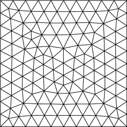
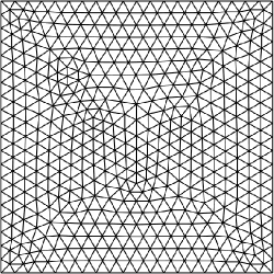
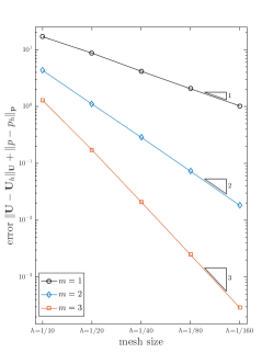
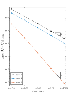
to show the convergence rates of our method. The source term $\boldsymbol{f}$ and the Dirichlet data $\boldsymbol{g}$ are taken accordingly. We employ a series of triangular meshes with mesh size $h=1/10,1/20,\ldots,1/160$, see Fig. 2. The numerical results are displayed in Fig. 3 and Fig. 4. For the first part (4.1), we plot the numerical error under energy norm $\|\boldsymbol{\mathrm{U}}-\boldsymbol{\mathrm{U}}_{h}\|_{\boldsymbol{\mathrm{U}}}+\|p-p_{h}\|_{\boldsymbol{\mathrm{p}}}$ in Fig. 3, which approaches zero at the speed $O(h^{m})$. The convergence rates are consistent with the theoretical analysis (4.22). For $L^{2}$ error, we also plot the errors $\|\boldsymbol{\mathrm{U}}-\boldsymbol{\mathrm{U}}_{h}\|_{L^{2}(\Omega)}$ and $\|p-p_{h}\|_{L^{2}(\Omega)}$ in Fig. 3, and we numerically detect the odd/even situation. For odd $m$, the $L^{2}$ errors converge to zero at the optimal speed, and for even $m$, the errors have a sub-optimal convergence rate. For the second system (4.23), we show the numerical results in Fig. 4. Clearly, the error under energy norm $\|\cdot\|_{\boldsymbol{\mathrm{u}}}$ converges to zero with the rate $O(h^{m})$ as the mesh size approaches $0$. For the $L^{2}$ norm, we also observe the optimal rate and sub-optimal rate for odd $m$ and even $m$, respectively. We note that the convergence orders under all error measurements are in perfect agreement with our theoretical error estimates.

Figure 2. The triangular meshes with mesh size $h=1/10$ (left) / $h=1/20$ (right) for Example 1.

Figure 3. The convergence rates of $\|\boldsymbol{\mathrm{U}}-\boldsymbol{\mathrm{U}}_{h}\|_{\boldsymbol{\mathrm{U}}}+\|p-p_{h}\|_{\boldsymbol{\mathrm{p}}}$ (left) / $\|\boldsymbol{\mathrm{U}}-\boldsymbol{\mathrm{U}}_{h}\|_{L^{2}(\Omega)}$ (middle) / $\|p-p_{h}\|_{L^{2}(\Omega)}$ (right) for Example 1.

Figure 4. The convergence rates of $\|\boldsymbol{u}-\boldsymbol{u}_{h}\|_{\boldsymbol{\mathrm{u}}}$ (left) / $\|\boldsymbol{u}-\boldsymbol{u}_{h}\|_{L^{2}(\Omega)}$ (right) for Example 1.

Example 2.

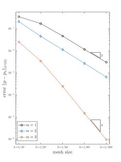
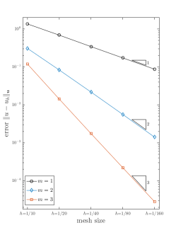
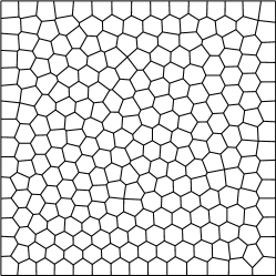
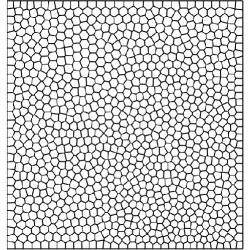
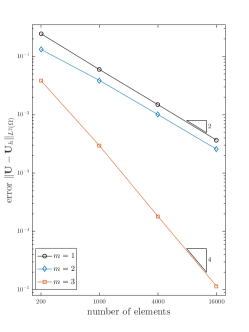
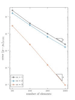
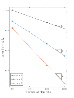
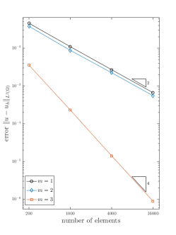
Here we solve the Stokes problem to show the great flexibility of the proposed method. The exact solution and the computational domain are taken the same as in Example 1 but in the example we use a series of polygonal meshes with $250$, $1000$, $4000$, $16000$ elements. These meshes consist of very general elements and are generated by PolyMesher[30], see Fig. 5. The numerical errors under all error measurements for both two systems (4.1) and (4.23) are shown in Fig. 6 and Fig. 7, respectively. Again we observe the optimal convergence orders for all energy norms. For $L^{2}$ norm, the odd/even situation is still detected. On such polygonal meshes, the numerically computed orders agree with our error estimates.

Figure 5. The polygonal meshes with 250 elements (left) / 1000 elements (right) for Example 2.

Figure 6. The convergence rates of $\|\boldsymbol{\mathrm{U}}-\boldsymbol{\mathrm{U}}_{h}\|_{\boldsymbol{\mathrm{U}}}+\|p-p_{h}\|_{\boldsymbol{\mathrm{p}}}$ (left) / $\|\boldsymbol{\mathrm{U}}-\boldsymbol{\mathrm{U}}_{h}\|_{L^{2}(\Omega)}$ (middle) / $\|p-p_{h}\|_{L^{2}(\Omega)}$ (right) for Example 2.

Figure 7. The convergence rates of $\|\boldsymbol{u}-\boldsymbol{u}_{h}\|_{\boldsymbol{\mathrm{u}}}$ (left) / $\|\boldsymbol{u}-\boldsymbol{u}_{h}\|_{L^{2}(\Omega)}$ (right) for Example 2.

Example 3.

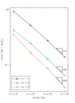
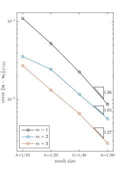
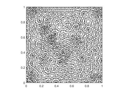
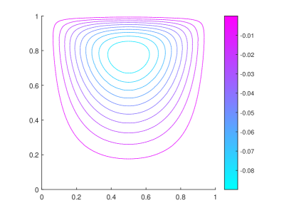
In this example, we test the modified lid-driven cavity problem [28] to investigate the performance of our method dealing with the problem with low regularities. We consider the unit square domain $\Omega=(0,1)^{2}$, which is subjected to a horizontal flow on the boundary $y=1$ with the velocity $\boldsymbol{u}(x,y)=(4x(1-x),0)^{T}$. The condition of remaining boundaries is no-slip boundary condition. The source term $\boldsymbol{f}$ is selected to be $(0,0)^{T}$. The velocity field on the upper boundary involves singularity in the upper right and left corners, but the restraints are not as strong as for the well-known standard lid-driven cavity problem [28]. We solve this problem on the triangular partition with $h=1/10$, $h=1/20$, $h=1/40$ and $h=1/80$, see Fig. 2. Since the analytical solution is unknown and we take the numerical solution which is obtained with the mesh size $h=1/320$ and the accuracy $m=3$ as the exact solution. The numerical errors in approximation to the velocity are presented in Fig. 8. The convergence rates under energy norms and $L^{2}$ norms are detected to be $O(h)$ for all accuracy $1\leq m\leq 3$. A possible explanation of such convergence rates can be traced back to the low regularity of this problem. Figure 9 and Figure 10 present the numerical results obtained on the mesh level $h=1/80$ with the accuracy $m=2$ and $m=3$, respectively. We can observe the main vortex in the center of the domain and two small vortices in the bottom left and right corners.

Figure 8. The convergence rates of $\|\boldsymbol{u}-\boldsymbol{u}_{h}\|_{\boldsymbol{\mathrm{u}}}$ (left) / $\|\boldsymbol{u}-\boldsymbol{u}_{h}\|_{L^{2}(\Omega)}$ (right) for Example 3.

Figure 9. Velocity vectors (left) and the streamline of the flow (right) with the accuracy $m=2$ for Example 3.

Figure 10. Velocity vectors (left) and the streamline of the flow (right) with the accuracy $m=3$ for Example 3.

5.2. 3D Example

Example 4.

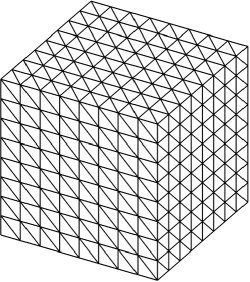
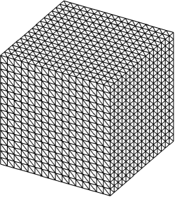
In this example, we consider the Stokes problem in three dimensions. We solve the problem on the domain $\Omega=(0,1)^{3}$ and we take a series of tetrahedral meshes with the resolution $h=1/4$, $h=1/8$ and $h=1/16$ (see Fig. 11). We choose the analytical solution $\boldsymbol{u}$ and $p$ as

$$\boldsymbol{u}(x,y,z)=\begin{bmatrix}1-e^{x}\cos(2\pi y)\\ \frac{1}{2\pi}e^{x}\sin(2\pi y)\\ 0\\ \end{bmatrix},\quad p(x,y,z)=x^{2}+y^{2}-\frac{2}{3}.$$

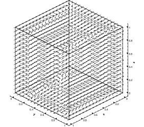
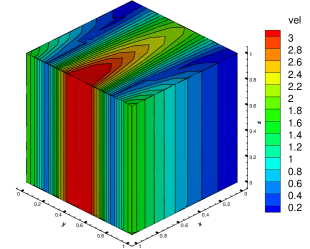
The numerical errors in approximation to the gradient and the pressure are collected in Tab. 2, and the numerical errors in solving the second first-order system are gathered in Tab. 3. We also depict the velocity field and the contour of $|\boldsymbol{u}_{h}|$ in Fig. 12 and the numerical solution in this figure is obtained on the mesh level $h=1/16$ with the accuracy $m=3$. Here, we still observe the odd/even situation. For odd $m$, the errors under $L^{2}$ norm seem to converge to zero optimally as the mesh size tends to zero. For even $m$, the convergence rates for all variables under $L^{2}$ norm are numerically detected to be sub-optimal. Again we note that all computed convergence orders are consistent with theoretical analysis.

Figure 11. The tetrahedral meshes with mesh size $h=1/8$ (left) / mesh size $h=1/16$ (right) for three-dimensional examples.

Figure 12. The velocity field (left) / the contour of $|\boldsymbol{u}_{h}|$ (right) for Example 4.

$m$	$h$	$\|\boldsymbol{\mathrm{U}}-\boldsymbol{\mathrm{U}}_{h}\|_{\boldsymbol{\mathrm{U}}}+\|p-p_{h}\|_{\boldsymbol{\mathrm{p}}}$	order	$\|\boldsymbol{\mathrm{U}}-\boldsymbol{\mathrm{U}}_{h}\|_{L^{2}(\Omega)}$	order	$\|p-p_{h}\|_{L^{2}(\Omega)}$	order
$1$	$1/4$	4.162e+1	-	2.022e-0	-	3.421e-0	-
	$1/8$	2.446e+1	0.77	9.998e-1	1.02	1.743e-0	0.97
	$1/16$	1.206e+1	1.02	3.653e-1	1.46	7.143e-1	1.29
$2$	$1/4$	1.476e+1	-	6.388e-1	-	1.053e-0	-
	$1/8$	4.213e-0	1.81	1.284e-1	2.31	3.425e-1	1.62
	$1/16$	1.167e-0	1.92	3.128e-2	2.03	7.752e-2	2.13
$3$	$1/4$	4.125e-0	-	1.557e-1	-	1.409e-1	-
	$1/8$	4.913e-1	3.06	1.125e-2	3.79	1.010e-2	3.80
	$1/16$	5.431e-2	3.13	7.507e-4	3.91	6.931e-4	3.86

Table 2. The numerical results of $\|\boldsymbol{\mathrm{U}}-\boldsymbol{\mathrm{U}}_{h}\|_{\boldsymbol{\mathrm{U}}}+\|p-p_{h}\|_{\boldsymbol{\mathrm{p}}}$, $\|\boldsymbol{\mathrm{U}}-\boldsymbol{\mathrm{U}}_{h}\|_{L^{2}(\Omega)}$ and $\|p-p_{h}\|_{L^{2}(\Omega)}$ for Example 4.

$m$	$h$	$\|\boldsymbol{u}-\boldsymbol{u}_{h}\|_{\boldsymbol{\mathrm{u}}}$	order	$\|\boldsymbol{u}-\boldsymbol{u}_{h}\|_{L^{2}(\Omega)}$	order
$1$	$1/4$	3.495e-0	-	2.865e-1	-
	$1/8$	2.075e-0	0.75	1.278e-1	1.16
	$1/16$	1.062e-0	0.97	5.081e-2	1.33
$2$	$1/4$	2.395e-0	-	1.509e-1	-
	$1/8$	5.402e-1	2.15	3.259e-2	2.21
	$1/16$	1.367e-1	1.98	7.653e-3	2.09
$3$	$1/4$	4.640e-1	-	2.307e-2	-
	$1/8$	5.382e-2	3.10	1.747e-3	3.72
	$1/16$	6.649e-3	3.02	1.255e-4	3.81

Table 3. The numerical results of $\|\boldsymbol{u}-\boldsymbol{u}_{h}\|_{\boldsymbol{\mathrm{u}}}$ and $\|\boldsymbol{u}-\boldsymbol{u}_{h}\|_{L^{2}(\Omega)}$ for Example 4.

Example 5.

In the last example, we solve another three-dimensional test problem. The domain and the meshes are selected the same as the previous example. For this test, the exact solution is

$$\boldsymbol{u}(x,y,z)=\begin{bmatrix}\sin(\pi x)\cos(\pi y)e^{-2z}\\ \cos(\pi x)\sin(\pi y)e^{-2z}\\ \pi\cos(\pi x)\cos(\pi y)e^{-2z}\\ \end{bmatrix},\quad p(x,y,z)=x^{2}+y^{2}+z^{2}-1,$$

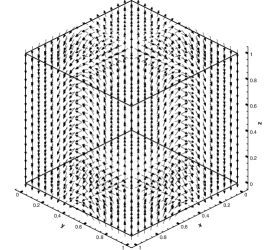
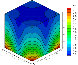
and the source term and the boundary data are taken from $\boldsymbol{u}$ and $p$. We list the numerical errors in approximation to the gradient of the velocity and pressure in Tab. 4 and the numerical errors of the velocity are given in Tab. 5. It can be clearly seen that the convergence rates for all unknowns are optimal under energy norms, and the old/even situation of $L^{2}$ errors is also observed. In addition, we plot the numerical solution with the mesh resolution $h=1/16$ and the accuracy $m=3$ to show the velocity field and the contour of $|\boldsymbol{u}_{h}|$ in Fig. 13.

Figure 13. The velocity field (left) / the contour of $|\boldsymbol{u}_{h}|$ (right) for Example 5.

$m$	$h$	$\|\boldsymbol{\mathrm{U}}-\boldsymbol{\mathrm{U}}_{h}\|_{\boldsymbol{\mathrm{U}}}+\|p-p_{h}\|_{\boldsymbol{\mathrm{p}}}$	order	$\|\boldsymbol{\mathrm{U}}-\boldsymbol{\mathrm{U}}_{h}\|_{L^{2}(\Omega)}$	order	$\|p-p_{h}\|_{L^{2}(\Omega)}$	order
$1$	$1/4$	7.312e-0	-	3.516e-1	-	1.932e-1	-
	$1/8$	3.691e-0	0.98	1.101e-1	1.67	9.032e-2	1.10
	$1/16$	1.831e-0	1.01	3.105e-2	1.82	3.132e-2	1.53
$2$	$1/4$	1.946e-0	-	5.619e-2	-	7.300e-2	-
	$1/8$	5.082e-1	1.93	1.163e-2	2.27	1.921e-2	1.92
	$1/16$	1.287e-1	1.98	2.646e-3	2.12	4.932e-3	1.98
$3$	$1/4$	7.028e-1	-	2.878e-2	-	2.609e-2	-
	$1/8$	7.992e-2	3.13	1.881e-3	3.93	1.848e-3	3.82
	$1/16$	9.250e-4	3.11	1.181e-4	4.01	1.093e-4	4.08

Table 4. The numerical results of $\|\boldsymbol{\mathrm{U}}-\boldsymbol{\mathrm{U}}_{h}\|_{\boldsymbol{\mathrm{U}}}+\|p-p_{h}\|_{\boldsymbol{\mathrm{p}}}$, $\|\boldsymbol{\mathrm{U}}-\boldsymbol{\mathrm{U}}_{h}\|_{L^{2}(\Omega)}$ and $\|p-p_{h}\|_{L^{2}(\Omega)}$ for Example 5.

$m$	$h$	$\|\boldsymbol{u}-\boldsymbol{u}_{h}\|_{\boldsymbol{\mathrm{u}}}$	order	$\|\boldsymbol{u}-\boldsymbol{u}_{h}\|_{L^{2}(\Omega)}$	order
$1$	$1/4$	1.217e-0	-	6.262e-2	-
	$1/8$	6.123e-1	0.99	2.155e-2	1.53
	$1/16$	3.041e-1	1.00	6.256e-3	1.78
$2$	$1/4$	3.311e-1	-	1.839e-2	-
	$1/8$	8.045e-2	2.04	3.552e-3	2.37
	$1/16$	1.975e-2	2.02	7.529e-4	2.23
$3$	$1/4$	1.157e-1	-	6.098e-3	-
	$1/8$	1.336e-2	3.11	3.874e-4	3.97
	$1/16$	1.561e-3	3.09	2.357e-5	4.03

Table 5. The numerical results of $\|\boldsymbol{u}-\boldsymbol{u}_{h}\|_{\boldsymbol{\mathrm{u}}}$ and $\|\boldsymbol{u}-\boldsymbol{u}_{h}\|_{L^{2}(\Omega)}$ for Example 5.

6. Conclusion

We constructed three types of approximation spaces by patch reconstructions. These reconstructed discontinuous spaces allow us to numerically solve the Stokes problem in two sequential steps. In the three spaces, the gradient of velocity, the velocity and the pressure are approximated, respectively. We first employed a reconstructed space that consists of piecewise curl-free polynomials with zero trace to approximate the gradient of the velocity and the pressure. Then we obtained the approximation to the velocity in the reconstructed piecewise divergence-free space. The convergence rates for all unknowns under $L^{2}$ norms and energy norms are derived. We presented a series of numerical tests in two and three dimensions to verify the error estimates and illustrate the great flexibility of the method we proposed. In addition, the computer program is able to handle approximation spaces of any high order and the elements with various geometry in a uniform manner.

Appendix A

In Appendix, we present the detailed computer implementation of constructing the approximation spaces introduced in Section 3. The construction contains two steps that are constructing element patches and solving local least squares problems on every element. We first give the recursive algorithm to the construction of the element patch, see Alg. 1.

Algorithm 1 Construction to Element Patch

0:  a partition $\mathcal{T}_{h}$ and a threshold $\#S$;

0:  the element patch of each element in $\mathcal{T}_{h}$;

1:  for every $K\in\mathcal{T}_{h}$ do

2:     initialize $t=0$, $S_{t}(K)=\left\{K\right\}$;

3:     while the cardinality of $S_{t}(K)<\#S$ do

4:        set $S_{t+1}(K)=S_{t}(K)$;

5:        for every $\widetilde{K}\in S_{t}(K)$ do

6:           add all adjacent face-neighbouring elements of $\widetilde{K}$ to $S_{t+1}(K)$;

7:        end for

8:        let $t=t+1$;

9:     end while

10:     collect collocation points of all elements in $S_{t}(K)$ in $\mathcal{I}(K)$;

11:     sort the distances between points in $\mathcal{I}(K)$ and $\boldsymbol{x}_{K}$;

12:     select the $\#S$ smallest values and collect the corresponding elements to form $S(K)$;

13:  end for

Then we will explain how to solve the least squares problems (3.1), (3.7) and (3.10). The key of solving least squares problems is to construct a group of polynomial bases that satisfy the constraints in (3.7) and (3.10). For (3.7), we shall construct the bases of the divergence-free polynomial space, that is $\mathbb{P}_{k}(D)^{d}\cap\boldsymbol{\mathrm{S}}^{0}(D)$, here $D$ is a bounded domain and $k$ is a positive integer. In two dimensions, we can directly take the curl of the natural polynomial bases

$$1,x,y,x^{2},xy,y^{2},x^{3},x^{2}y,xy^{2},y^{3},\ldots$$

to obtain the bases of divergence-free polynomials, as illustrated in [2]. For example, if the linear accuracy is considered we have that

$$\mathbb{P}_{1}(D)^{2}\cap\boldsymbol{\mathrm{S}}^{0}(D)=\text{span}\left\{\begin{bmatrix}1\\ 0\\ \end{bmatrix},\begin{bmatrix}0\\ 1\\ \end{bmatrix},\begin{bmatrix}0\\ x\\ \end{bmatrix},\begin{bmatrix}y\\ 0\\ \end{bmatrix},\begin{bmatrix}x\\ -y\\ \end{bmatrix}\right\}.$$

For the second-order case, it is easy to find that

$$\mathbb{P}_{2}(D)^{2}\cap\boldsymbol{\mathrm{S}}^{0}(D)=\text{span}\left\{\begin{bmatrix}1\\ 0\\ \end{bmatrix},\begin{bmatrix}0\\ 1\\ \end{bmatrix},\begin{bmatrix}0\\ x\\ \end{bmatrix},\begin{bmatrix}y\\ 0\\ \end{bmatrix},\begin{bmatrix}x\\ -y\\ \end{bmatrix},\begin{bmatrix}0\\ x^{2}\\ \end{bmatrix},\begin{bmatrix}x^{2}\\ -2xy\\ \end{bmatrix},\begin{bmatrix}-2xy\\ y^{2}\\ \end{bmatrix},\begin{bmatrix}y^{2}\\ 0\\ \end{bmatrix}\right\}.$$

To get a group of divergence-free polynomials bases in three dimensions is a bit more complicated and we outline a method which is easy to implement. We construct two groups of polynomials $\widetilde{\boldsymbol{\mathrm{S}}}_{k}^{1}(D)$ and $\widetilde{\boldsymbol{\mathrm{S}}}_{k}^{2}(D)$ whose union actually forms a group of bases. The first group $\widetilde{\boldsymbol{\mathrm{S}}}_{k}^{1}(D)$ consists of the vector-valued polynomials which only have one nonzero entry. Specifically speaking, $\widetilde{\boldsymbol{\mathrm{S}}}_{k}^{1}(D)$ has three types of polynomials, that is $\widetilde{\boldsymbol{\mathrm{S}}}_{k}^{1}(D)=\boldsymbol{\mathrm{Q}}_{k}^{1}(D)\cup\boldsymbol{\mathrm{Q}}_{k}^{2}(D)\cup\boldsymbol{\mathrm{Q}}_{k}^{3}(D)$, where

(A.1) $$\boldsymbol{\mathrm{Q}}_{k}^{1}(D):=\left\{\boldsymbol{p}=(p_{1},0,0)^{T}\in\mathbb{P}_{k}(D)^{3}\ |\ p_{1}(y,z)\in\mathbb{P}_{k}(y,z)\right\},$$

$$\boldsymbol{\mathrm{Q}}_{k}^{2}(D):=\left\{\boldsymbol{p}=(0,p_{2},0)^{T}\in\mathbb{P}_{k}(D)^{3}\ |\ p_{2}(x,z)\in\mathbb{P}_{k}(x,z)\right\},$$

$$\boldsymbol{\mathrm{Q}}_{k}^{3}(D):=\left\{\boldsymbol{p}=(0,0,p_{3})^{T}\in\mathbb{P}_{k}(D)^{3}\ |\ p_{3}(y,z)\in\mathbb{P}_{k}(x,y)\right\},$$

and $\mathbb{P}_{k}(a,b)$ denotes the polynomial space of degree $k$ based on the coordinate $(a,b)$,

$$\mathbb{P}_{k}(a,b)=\text{span}\left\{1,a,b,a^{2},ab,b^{2},\ldots,a^{k},a^{k-1}b,\ldots,ab^{k-1},b^{k}\right\}.$$

Then $\widetilde{\boldsymbol{\mathrm{S}}}_{k}^{2}(D)$ has two types of polynomials, that is $\widetilde{\boldsymbol{\mathrm{S}}}_{k}^{2}(D)=\boldsymbol{\mathrm{R}}_{k}^{1}(D)\cup\boldsymbol{\mathrm{R}}_{k}^{2}(D)$, where

(A.2) $$\boldsymbol{\mathrm{R}}_{k}^{1}(D):=\bigg{\{}\boldsymbol{p}=(p_{1},p_{2},0)^{T}\in\mathbb{P}_{k}(D)^{3}\ \big{|}\ p_{1}=x^{t}q, \ p_{2}=-\int q(y,z)dy,$$

$$q(y,z) \in\mathbb{P}_{k-t}(y,z),\ 1\leq t\leq k\bigg{\}},$$

$$\boldsymbol{\mathrm{R}}_{k}^{2}(D):=\bigg{\{}\boldsymbol{p}=(p_{1},0,p_{3})^{T}\in\mathbb{P}_{k}(D)^{3}\ \big{|}\ p_{1}=x^{t}q, \ p_{3}=-\int q(y,z)dz,$$

$$q(y,z) \in\mathbb{P}_{k-t}(y,z),\ 1\leq t\leq k\bigg{\}}.$$

It is trivial to verify that the polynomials in $\widetilde{\boldsymbol{\mathrm{S}}}_{k}^{1}(D)$ and $\widetilde{\boldsymbol{\mathrm{S}}}_{k}^{2}(D)$ are divergence-free, and we state the following lemma.

Lemma A.1.

The divergence-free polynomial space $\mathbb{P}_{k}(D)^{3}\cap\boldsymbol{\mathrm{S}}^{0}(D)$ satisfies that $\mathbb{P}_{k}(D)^{3}\cap\boldsymbol{\mathrm{S}}^{0}(D)=\widetilde{\boldsymbol{\mathrm{S}}}_{k}^{1}(D)\cup\widetilde{\boldsymbol{\mathrm{S}}}_{k}^{2}(D)$.

Proof.

We let $\boldsymbol{q}\in\mathbb{P}_{k}(D)^{3}$ such that $\boldsymbol{q}=\widetilde{\boldsymbol{\mathrm{S}}}_{k}^{1}(D)\cap\widetilde{\boldsymbol{\mathrm{S}}}_{k}^{2}(D)$. By the definition (A.1), the first entry of $\boldsymbol{q}$ only depends on $y$ and $z$. From (A.2), the first entry of $\boldsymbol{q}$ must rely on $x$, which gives $\boldsymbol{q}=\boldsymbol{0}$. Hence, we have that $\widetilde{\boldsymbol{\mathrm{S}}}_{k}^{1}(D)\cap\widetilde{\boldsymbol{\mathrm{S}}}_{k}^{2}(D)=\left\{\boldsymbol{0}\right\}$. From (A.1) and (A.2), we can know that $\text{dim}(\widetilde{\boldsymbol{\mathrm{S}}}_{k}^{1}(D))=3(k+2)(k+1)/2$ and $\text{dim}(\widetilde{\boldsymbol{\mathrm{S}}}_{k}^{2}(D))=(k+2)(k+1)k/3$. By [2], we have that $\text{dim}(\mathbb{P}_{k}(D)^{3}\cap\boldsymbol{\mathrm{S}}^{0}(D))=3C_{k+3}^{3}-C_{k+2}^{3}$, which exactly implies $\text{dim}(\mathbb{P}_{k}(D)^{3}\cap\boldsymbol{\mathrm{S}}^{0}(D))=\text{dim}(\widetilde{\boldsymbol{\mathrm{S}}}_{k}^{1}(D))+\text{dim}(\widetilde{\boldsymbol{\mathrm{S}}}_{k}^{2}(D))$. This fact gives us that $\mathbb{P}_{k}(D)^{3}\cap\boldsymbol{\mathrm{S}}^{0}(D)=\widetilde{\boldsymbol{\mathrm{S}}}_{k}^{1}(D)\cup\widetilde{\boldsymbol{\mathrm{S}}}_{k}^{2}(D)$ and completes the proof. ∎

Further, we give an example of the linear accuracy. In this case, we can obtain that

$$\widetilde{\boldsymbol{\mathrm{S}}}_{1}^{1}(D)=\text{span}\left\{\begin{bmatrix}1\\ 0\\ 0\\ \end{bmatrix},\begin{bmatrix}0\\ 1\\ 0\\ \end{bmatrix},\begin{bmatrix}0\\ 0\\ 1\\ \end{bmatrix},\begin{bmatrix}y\\ 0\\ 0\\ \end{bmatrix},\begin{bmatrix}z\\ 0\\ 0\\ \end{bmatrix},\begin{bmatrix}0\\ x\\ 0\\ \end{bmatrix},\begin{bmatrix}0\\ z\\ 0\\ \end{bmatrix},\begin{bmatrix}0\\ 0\\ y\\ \end{bmatrix},\begin{bmatrix}0\\ 0\\ z\\ \end{bmatrix}\right\},$$

and

$$\widetilde{\boldsymbol{\mathrm{S}}}_{2}^{2}(D)=\text{span}\left\{\begin{bmatrix}x\\ -y\\ 0\\ \end{bmatrix},\begin{bmatrix}x\\ 0\\ -z\\ \end{bmatrix}\right\}.$$

Hence, $\mathbb{P}_{1}(D)^{3}\cap\boldsymbol{\mathrm{S}}^{0}(D)=\widetilde{\boldsymbol{\mathrm{S}}}_{1}^{1}(D)\cup\widetilde{\boldsymbol{\mathrm{S}}}_{1}^{2}(D)$.

Then we consider to solve the problem (3.10), which requires us to construct the polynomial space consists of the curl-free polynomials with zero trace, that is $\mathbb{P}_{k}(D)^{d\times d}\cap\boldsymbol{\mathrm{I}}^{0}(D)$. Actually after obtaining the bases of the divergence-free polynomial space, it is easy to get the bases of the polynomial space $\mathbb{P}_{k}(D)^{d\times d}\cap\boldsymbol{\mathrm{I}}^{0}(D)$. We can take the gradient of the divergence-free polynomial bases to get those bases. Again we take $k=1$ for an example and we can obtain that

$$\mathbb{P}_{1}(D)^{d\times d}\cap\boldsymbol{\mathrm{I}}^{0}(D)=\text{span}\left\{\begin{bmatrix}0&1\\ 0&0\\ \end{bmatrix},\begin{bmatrix}0&0\\ 1&0\\ \end{bmatrix},\begin{bmatrix}1&0\\ 0&-1\\ \end{bmatrix},\begin{bmatrix}0&x\\ 0&0\\ \end{bmatrix},\begin{bmatrix}x&-y\\ 0&-x\\ \end{bmatrix},\begin{bmatrix}-y&0\\ -x&y\\ \end{bmatrix},\begin{bmatrix}0&0\\ y&0\\ \end{bmatrix}\right\}.$$

In the rest of Appendix, we present the details of the computer implementation to the reconstructed space. Let us construct the space $\boldsymbol{\mathrm{I}}_{h}^{1}$ in two dimensions as an illustration. We consider the element $K_{0}$ and we let its element patch $S(K_{0})$ formed by its face-neighbouring elements, see Fig. 14.

Figure 14. $K_{0}$ and its neighbours (left) / collocation points (right).

For a tensor-valued function $\boldsymbol{g}=(g_{00},g_{01};g_{10},g_{11})^{T}\in\boldsymbol{\mathrm{U}}_{h}(g_{00}=-g_{11})$, the least squares problem (3.7) on $S(K_{0})$ takes the form

(A.3) $$\widehat{\mathcal{R}}_{K_{0}}^{1}\boldsymbol{g}=\mathop{\arg\min}_{\boldsymbol{q}\in\mathbb{P}_{m}(S(K_{0}))^{2\times}\cap\boldsymbol{\mathrm{I}}^{0}(S(K_{0}))}\sum_{\boldsymbol{x}\in\mathcal{I}(K_{0})}\|\boldsymbol{q}(\boldsymbol{x})-\boldsymbol{g}(\boldsymbol{x})\|^{2}_{l^{2}\times l^{2}},\quad\text{s.t. }\boldsymbol{q}(\boldsymbol{x}_{K_{0}})=\boldsymbol{g}(\boldsymbol{x}_{K_{0}}).$$

From the bases of the polynomial space $\mathbb{P}_{1}(S(K_{0}))^{2}\cap\boldsymbol{\mathrm{I}}^{0}(S(K))$, the polynomial $\boldsymbol{p}(\boldsymbol{x})$ in (A.3) has the form

$$\boldsymbol{p}(\boldsymbol{x})=a_{0}\begin{bmatrix}1&0\\ 0&-1\\ \end{bmatrix}+a_{1}\begin{bmatrix}0&0\\ 1&0\\ \end{bmatrix}+ a_{2}\begin{bmatrix}0&1\\ 0&0\\ \end{bmatrix}$$

$$+a_{3}\begin{bmatrix}0&x\\ 0&0\\ \end{bmatrix}+ a_{4}\begin{bmatrix}x&-y\\ 0&-x\\ \end{bmatrix}+a_{5}\begin{bmatrix}-y&0\\ -x&y\\ \end{bmatrix}+a_{6}\begin{bmatrix}0&0\\ y&0\\ \end{bmatrix}.$$

By the constraint in (A.3), we can know the values of $a_{0}$, $a_{1}$ and $a_{2}$ and we rewrite the polynomial $\boldsymbol{p}(\boldsymbol{x})$ as

$$\boldsymbol{p}(\boldsymbol{x})=\begin{bmatrix}g_{00}(\boldsymbol{x}_{K_{0}})&g_{01}(\boldsymbol{x}_{K_{0}})\\ g_{10}(\boldsymbol{x}_{K_{0}})&g_{11}(\boldsymbol{x}_{K_{0}})\\ \end{bmatrix}+ a_{0}\begin{bmatrix}0&x-x_{K_{0}}\\ 0&0\\ \end{bmatrix}+a_{1}\begin{bmatrix}x-x_{K_{0}}&-y+y_{K_{0}}\\ 0&-x+x_{K_{0}}\\ \end{bmatrix}$$

$$+ a_{2}\begin{bmatrix}-y+y_{K_{0}}&0\\ -x+x_{K_{0}}&y-y_{K_{0}}\\ \end{bmatrix}+a_{3}\begin{bmatrix}0&0\\ y-y_{K_{0}}&0\\ \end{bmatrix},$$

where $\boldsymbol{x}_{K_{i}}=(x_{K_{i}},y_{K_{i}})(0\leq i\leq 3)$. Thus the problem (A.3) is equivalent to

(A.4) $$\mathop{\arg\min}_{a_{3},a_{4},a_{5},a_{6}\in\mathbb{R}}\sum_{i=1}^{3} \bigg{\|}a_{3}\begin{bmatrix}0&x_{K_{i}}-x_{K_{0}}\\ 0&0\\ \end{bmatrix}+a_{4}\begin{bmatrix}x_{K_{i}}-x_{K_{0}}&-y_{K_{i}}+y_{K_{0}}\\ 0&-x_{K_{i}}+x_{K_{0}}\\ \end{bmatrix}+a_{5}\begin{bmatrix}-y_{K_{i}}+y_{K_{0}}&0\\ -x_{K_{i}}+x_{K_{0}}&y_{K_{i}}-y_{K_{0}}\\ \end{bmatrix}$$

$$+ a_{6}\begin{bmatrix}0&0\\ y_{K_{i}}-y_{K_{0}}&0\\ \end{bmatrix}-\begin{bmatrix}g_{00}(\boldsymbol{x}_{K_{i}})-g_{00}(\boldsymbol{x}_{K_{0}})&g_{01}(\boldsymbol{x}_{K_{i}})-g_{01}(\boldsymbol{x}_{K_{0}})\\ g_{10}(\boldsymbol{x}_{K_{i}})-g_{10}(\boldsymbol{x}_{K_{0}})&g_{11}(\boldsymbol{x}_{K_{i}})-g_{11}(\boldsymbol{x}_{K_{0}})\\ \end{bmatrix}\bigg{\|}^{2}_{l^{2}\times l^{2}}.$$

The solution to (A.4) reads

$$\begin{bmatrix}a_{3}\\ a_{4}\\ a_{5}\\ a_{6}\end{bmatrix}=(A^{T}A)^{-1}A^{T}\begin{bmatrix}2(g_{00}(\boldsymbol{x}_{K_{1}})-g_{00}(\boldsymbol{x}_{K_{0}}))\\ g_{01}(\boldsymbol{x}_{K_{1}})-g_{01}(\boldsymbol{x}_{K_{0}})\\ g_{10}(\boldsymbol{x}_{K_{1}})-g_{10}(\boldsymbol{x}_{K_{0}})\\ \cdots\\ 2(g_{00}(\boldsymbol{x}_{K_{3}})-g_{00}(\boldsymbol{x}_{K_{0}}))\\ g_{01}(\boldsymbol{x}_{K_{3}})-g_{01}(\boldsymbol{x}_{K_{0}})\\ g_{10}(\boldsymbol{x}_{K_{3}})-g_{10}(\boldsymbol{x}_{K_{0}})\\ \end{bmatrix},$$

where

$$A=\begin{bmatrix}0&2(x_{K_{1}}-x_{K_{0}})&-2(y_{K_{1}}-y_{K_{0}})&0\\ x_{K_{1}}-x_{K_{0}}&-y_{K_{1}}+y_{K_{0}}&0&0\\ 0&0&-x_{K_{1}}+x_{K_{0}}&y_{K_{1}}-y_{K_{0}}\\ \cdots&\cdots&\cdots&\cdots\\ 0&2(x_{K_{3}}-x_{K_{0}})&-2(y_{K_{3}}-y_{K_{0}})&0\\ x_{K_{3}}-x_{K_{0}}&-y_{K_{3}}+y_{K_{0}}&0&0\\ 0&0&-x_{K_{3}}+x_{K_{0}}&y_{K_{3}}-y_{K_{0}}\\ \end{bmatrix}.$$

By rearrangement, we can obtain the solution to (A.3), which takes the form

$$\begin{bmatrix}a_{0}\\ a_{1}\\ a_{2}\\ a_{3}\\ a_{4}\\ a_{5}\\ a_{6}\end{bmatrix}=\begin{bmatrix}I_{3\times 3}&0\\ -MI_{9\times 3}&M\\ \end{bmatrix}\begin{bmatrix}g_{00}(\boldsymbol{x}_{K_{0}})\\ g_{01}(\boldsymbol{x}_{K_{0}})\\ g_{10}(\boldsymbol{x}_{K_{0}})\\ \cdots\\ g_{00}(\boldsymbol{x}_{K_{3}})\\ g_{01}(\boldsymbol{x}_{K_{3}})\\ g_{10}(\boldsymbol{x}_{K_{3}})\\ \end{bmatrix},\quad M=(A^{T}A)^{-1}A^{T}\begin{bmatrix}2&0&0&0&0&0\\ 0&I_{2\times 2}&0&0&0&0\\ 0&0&2&0&0&0\\ 0&0&0&I_{2\times 2}&0&0\\ 0&0&0&0&2&0\\ 0&0&0&0&0&I_{2\times 2}\\ \end{bmatrix},$$

where $I_{2\times 2}$ and $I_{3\times 3}$ are $2\times 2$ identity matrix and $3\times 3$ identity matrix and $I_{9\times 3}=(I_{3\times 3},I_{3\times 3},I_{3\times 3})^{T}$. We note that the collocation points in $\mathcal{I}(K)$ totally determine the matrix $M$, and by the expansion (3.11), the coefficient matrix

(A.5) $$\begin{bmatrix}I_{3\times 3}&0\\ -MI_{9\times 3}&M\\ \end{bmatrix}$$

actually contains all information of the basis functions $\widehat{\boldsymbol{\lambda}}_{K_{i}}^{j,k}(0\leq i\leq 3,1\leq j,k\leq 2,j+k<4)$ on the element $K_{0}$. Then we can use the coefficient matrix (A.5) on each element to represent the reconstructed space $\boldsymbol{\mathrm{I}}^{1}_{h}$. For the spaces $U_{h}^{1}$ and $\boldsymbol{\mathrm{S}}_{h}^{1}$, their constructions are very similar. In addition, such a computer implementation can be easily adapted to three dimensions and the case when higher-order accuracy is considered.

References

- [1] D. N. Arnold, An interior penalty finite element method with discontinuous elements, SIAM J. Numer. Anal. 19 (1982), no. 4, 742–760.
- [2] G. A. Baker, W. N. Jureidini, and O. A. Karakashian, Piecewise solenoidal vector fields and the Stokes problem, SIAM J. Numer. Anal. 27 (1990), no. 6, 1466–1485.
- [3] Rickard Bensow and Mats G. Larson, Discontinuous least-squares finite element method for the div-curl problem, Numer. Math. 101 (2005), no. 4, 601–617.
- [4] Rickard E. Bensow and Mats G. Larson, Discontinuous/continuous least-squares finite element methods for elliptic problems, Math. Models Methods Appl. Sci. 15 (2005), no. 6, 825–842.
- [5] Fleurianne Bertrand, Zhiqiang Cai, and Eun Young Park, Least-squares methods for elasticity and Stokes equations with weakly imposed symmetry, Comput. Methods Appl. Math. 19 (2019), no. 3, 415–430.
- [6] Pavel Bochev, James Lai, and Luke Olson, A locally conservative, discontinuous least-squares finite element method for the Stokes equations, Internat. J. Numer. Methods Fluids 68 (2012), no. 6, 782–804.
- [7] by same author, A non-conforming least-squares finite element method for incompressible fluid flow problems, Internat. J. Numer. Methods Fluids 72 (2013), no. 3, 375–402.
- [8] Pavel B. Bochev and Max D. Gunzburger, Analysis of least squares finite element methods for the Stokes equations, Math. Comp. 63 (1994), no. 208, 479–506.
- [9] by same author, Least-squares finite element methods, Applied Mathematical Sciences, vol. 166, Springer, New York, 2009.
- [10] D. Boffi, F. Brezzi, and M. Fortin, Mixed Finite Element Methods and Applications, Springer Series in Computational Mathematics, vol. 44, Springer, Heidelberg, 2013.
- [11] S. C. Brenner and L. R. Scott, The Mathematical Theory of Finite Element Methods, third ed., Texts in Applied Mathematics, vol. 15, Springer, New York, 2008.
- [12] Susanne C. Brenner, Poincaré-Friedrichs inequalities for piecewise functions, SIAM J. Numer. Anal. 41 (2003), no. 1, 306–324.
- [13] Franco Brezzi, Annalisa Buffa, and Konstantin Lipnikov, Mimetic finite differences for elliptic problems, M2AN Math. Model. Numer. Anal. 43 (2009), no. 2, 277–295.
- [14] Z. Cai, C.-O. Lee, T. A. Manteuffel, and S. F. McCormick, First-order system least squares for the Stokes and linear elasticity equations: further results, SIAM J. Sci. Comput. 21 (2000), no. 5, 1728–1739, Iterative methods for solving systems of algebraic equations (Copper Mountain, CO, 1998).
- [15] Z. Cai, T. A. Manteuffel, and S. F. McCormick, First-order system least squares for the Stokes equations, with application to linear elasticity, SIAM J. Numer. Anal. 34 (1997), no. 5, 1727–1741.
- [16] Zhiqiang Cai, Least squares for the perturbed Stokes equations and the Reissner-Mindlin plate, SIAM J. Numer. Anal. 38 (2000), no. 5, 1561–1581.
- [17] Vivette Girault and Pierre Arnaud Raviart, Finite element methods for navier-stokes equations: Theory and algorithms, Springer-Verlag, 1986.
- [18] J. J. Heys, E. Lee, T. A. Manteuffel, and S. F. McCormick, On mass-conserving least-squares methods, SIAM J. Sci. Comput. 28 (2006), no. 5, 1675–1693.
- [19] Bo-Nan Jiang and C. L. Chang, Least-squares finite elements for the Stokes problem, Comput. Methods Appl. Mech. Engrg. 78 (1990), no. 3, 297–311.
- [20] Ohannes A. Karakashian and Frederic Pascal, Convergence of adaptive discontinuous Galerkin approximations of second-order elliptic problems, SIAM J. Numer. Anal. 45 (2007), no. 2, 641–665.
- [21] R. B. Kellogg and J. E. Osborn, A regularity result for the Stokes problem in a convex polygon, J. Functional Analysis 21 (1976), no. 4, 397–431.
- [22] Ruo Li, Pingbing Ming, Ziyuan Sun, and Zhijian Yang, An arbitrary-order discontinuous Galerkin method with one unknown per element, J. Sci. Comput. 80 (2019), no. 1, 268–288.
- [23] Ruo Li, Pingbing Ming, and Fengyang Tang, An efficient high order heterogeneous multiscale method for elliptic problems, Multiscale Model. Simul. 10 (2012), no. 1, 259–283.
- [24] Ruo Li, Zhiyuan Sun, and Fanyi Yang, Solving eigenvalue problems in a discontinuous approximate space by patch reconstruction, SIAM J. Sci. Comput. 41 (2019), no. 5, A3381–A3400.
- [25] Ruo Li and Fanyi Yang, A least squares method for linear elasticity using a patch reconstructed space, Comput. Methods Appl. Mech. Engrg. 363 (2020), no. 1.
- [26] by same author, A sequential least squares method for Poisson equation using a patch reconstructed space, SIAM J. Numer. Anal. 58 (2020), no. 1, 353–374.
- [27] K. Liu, T. A. Manteuffel, S. F. McCormick, J. W. Ruge, and L. Tang, Hybrid first-order system least squares finite element methods with application to Stokes equations, SIAM J. Numer. Anal. 51 (2013), no. 4, 2214–2237.
- [28] Carina Nisters and Alexander Schwarz, Efficient stress-velocity least-squares finite element formulations for the incompressible Navier-Stokes equations, Comput. Methods Appl. Mech. Engrg. 341 (2018), 333–359.
- [29] Byeong-Chun Shin and Peyman Hessari, Least-squares spectral method for velocity-vorticity-pressure form of the Stokes equations, Numer. Methods Partial Differential Equations 32 (2016), no. 2, 661–680.
- [30] C. Talischi, G. H. Paulino, A. Pereira, and I. F. M. Menezes, PolyMesher: a general-purpose mesh generator for polygonal elements written in Matlab, Struct. Multidiscip. Optim. 45 (2012), no. 3, 309–328.