Holistically-Attracted Wireframe Parsing
Abstract
This paper presents a fast and parsimonious parsing method to accurately and robustly detect a vectorized wireframe in an input image with a single forward pass. The proposed method is end-to-end trainable, consisting of three components: (i) line segment and junction proposal generation, (ii) line segment and junction matching, and (iii) line segment and junction verification. For computing line segment proposals, a novel exact dual representation is proposed which exploits a parsimonious geometric reparameterization for line segments and forms a holistic 4-dimensional attraction field map for an input image. Junctions can be treated as the “basins” in the attraction field. The proposed method is thus called Holistically-Attracted Wireframe Parser (HAWP). In experiments, the proposed method is tested on two benchmarks, the Wireframe dataset [14] and the YorkUrban dataset [8]. On both benchmarks, it obtains state-of-the-art performance in terms of accuracy and efficiency. For example, on the Wireframe dataset, compared to the previous state-of-the-art method L-CNN [40], it improves the challenging mean structural average precision (msAP) by a large margin ( absolute improvements), and achieves 29.5 FPS on single GPU ( relative improvement). A systematic ablation study is performed to further justify the proposed method.
1 Introduction
1.1 Motivations and Objectives
Line segments and junctions are prominent visual patterns in the low-level vision, and thus often used as important cues/features to facilitate many downstream vision tasks such as camera pose estimation [23, 24, 10], image matching [35], image rectification [36], structure from motion (SfM) [4, 21], visual SLAM [18, 38, 41], and surface reconstruction [16]. Both line segment detection and junction detection remain challenging problems in computer vision [31, 33, 34]. Line segments and junctions are often statistically coupled in images. So, a new research task, wireframe parsing, is recently emerged to tackle the problem of jointly detecting meaningful and salient line segments and junctions with large-scale benchmarks available [14]. And, end-to-end trainable approaches based on deep neural networks (DNNs) are one of the most interesting frameworks, which have shown remarkable performance.
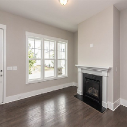
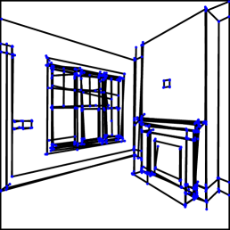
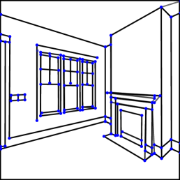
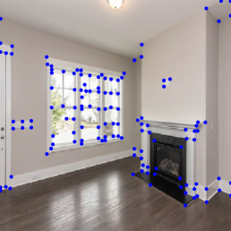
In wireframe parsing, it can be addressed relatively better to learn a junction detector with state-of-the-art deep learning approaches and the heatmap representation (inspired by its widespread use in human pose estimation [22, 28, 39]). This motivated a conceptually simple yet powerful wireframe parsing algorithm called L-CNN [40], which achieved state-of-the-art performance on the Wireframe benchmark [14]. L-CNN bypasses learning a line segment detector. It develops a sophisticated and carefully-crafted sampling schema to generate line segment proposals from all possible candidates based on the predicted junctions, and then utilizes a line segment verification module to classify the proposals. A large number of proposals are entailed for achieving good results at the expense of computational costs. And, ignoring line segment information in the proposal stage may not take full advantage of the deep learning pipeline for further improving performance.
On the other hand, without leveraging junction information in learning, the recently proposed attraction field map (AFM) based approaches [33, 34] are the state-of-the-art methods for line segment detection. AFM is not strictly end-to-end trainable. The reparameterization of pixels in the lifting process is for lines, instead of line segments (i.e., we can only infer a line with a given displacement vector, and that is why the squeezing module is needed).
In this paper, we are interested in learning an end-to-end trainable and fast wireframe parser. First, we aim to develop an exact dual and parsimonious reparameterization scheme for line segments, in a similar spirit to the AFM [33], but without resorting to the heuristic squeezing process in inference. Then, we aim to tackle wireframe parsing by leveraging both line segment and junction proposals to improve both accuracy and efficiency and to eliminate the carefully-crafted sampling schema as done in L-CNN [40].
1.2 Method Overview
In general, a parsing algorithm adopts two phases as proposed in the generic image parsing framework [27]: proposal generation and proposal verification, which are also realized in the state-of-the-art object detection and instance segmentation framework [11, 25, 13]. The current state-of-the-art wireframe parser, L-CNN [40] follows the two-phase parsing paradigm. The proposed method in this paper also adopts the same setup. As illustrated in Fig. 1 and Fig. 2, the proposed method consists of three components:
i) Proposal initialization: line segment detection and junction detection. Given an input image, it first passes through a shared feature backbone (e.g., the stacked Hourglass network [22]) to extract deep features. Then, for junction detection, we adopt the same head regressor based on the heatmap representation as done in L-CNN [40] (Section 4.2), from which the top- junctions are selected as initial junction proposals. For computing line segment proposals, a novel method is proposed (Section 4.1).
ii) Proposal refinement: line segment and junction matching. The matching is to calculate meaningful alignment between line segment initial proposals and junction initial proposals. In the refinement (Section 4.3), a line segment proposal is kept if its two end-points are supported by two junction proposals. If a junction proposal does not find any support line segment proposal, it will be removed.
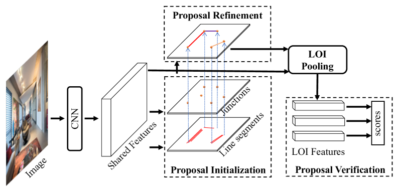
iii) Proposal verification: line segment and junction classification. The verification process is to classify (double-check) the line segments and junctions from the proposal refinement stage. We utilize the same verification head classifier (Section 4.4) as done in L-CNN [40], which exploits a Line-of-Interest (LOI) pooling operation to compute features for a line segment, motivated by the Region-of-Interest (ROI) pooling operation used in the popular two-stage R-CNN frameworks [11, 25, 13].
Geometrically speaking, the proposed wireframe parser is enabled by the holistic 4-D attraction field map and the “basins” of the attraction field revealed by junctions. We thus call the proposed method a Holistically-Attracted Wireframe Parser (HAWP). The proposed HAWP is end-to-end trainable and computes a vectorized wireframe for an input image in single forward pass. The key difference between our HAWP and the current state-of-the-art L-CNN [40] approach is the novel line segment reparameterization and its end-to-end integration in the parsing pipeline. Our HAWP outperforms L-CNN by a large margin in terms of both accuracy and efficiency (Section 5).
2 Related Work and Our Contributions
The fundamental problem in wireframe parsing is to learn to understand the basic physical and geometric constraints of our world. The problem can date back to the pioneering work of understanding Blocks World by Larry Roberts [26, 12] at the very beginning of computer vision. We briefly review two core aspects as follows.
Representation of Line Segments. There is a big gap between the mathematically simple geometric representation of line segments (at the symbol level) and the raw image data (at the signal level). A vast amount of efforts have been devoted to closing the gap with remarkable progress achieved. Roughly speaking, there are three-level representations of line segments developed in the literature: (i) Edge-pixel based representations, which are the classic approaches and have facilitated a tremendous number of line segment detectors [3, 20, 5, 9, 29, 7, 29, 2, 7]. Many of these line segment detectors suffer from two fundamental issues inherited from the underlying representations: the intrinsic uncertainty and the fundamental limit of edge detection, and the lack of structural information guidance from pixels to line segments. The first issue has been eliminated to some extent by state-of-the-art deep edge detection methods [32, 19]. (ii) Local support region based representations, e.g., the level-line based support region used in the popular LSD method [29] and its many variants [1, 7]. The local support region is still defined on top of local edge information (gradient magnitude and orientation), thus inheriting the fundamental limit. (iii) Global region partition based representation, which is recently proposed in the AFM method [33]. AFM does not depend on edge information, but entails powerful and computationally efficient DNNs in learning and inference. AFM is not strictly an exact line segment representation, but a global region partition based line representation. The issue is addressed in this paper by proposing a novel holistic AFM representation that is parsimonious and exact for line segments.
Wireframe Parsing Algorithm Design. The recent resurgence of wireframe parsing, especially in an end-to-end way, is driven by the remarkable progress of DNNs which enables holistic map-to-map prediction (e.g., from raw images to heatmaps directly encoding edges [32] or human keypoints [30], etc.). As aforementioned, the general framework of parsing is similar between different parsers. Depending on whether line segment representations are explicitly exploited or not, the recent work on wireframe parsing can be divided into two categories: (i) Holistic wireframe parsing, which include data-driven proposal generation for both line segments and junctions, e.g., the deep wireframe parser (DWP) [14] presented along with the wireframe benchmark. DWP is not end-to-end trainable and relatively slow. (ii) Deductive wireframe parsing, which utilizes data-driven proposals only for junctions and resorts to sophisticated top-down sampling methods to deduce line segments based on detected junctions, e.g., PPG-Net [37] and L-CNN [40]. The main drawbacks of deductive wireframe parsing are in two-fold: high computational expense for line segment verification, and over-dependence on junction prediction. The proposed HAWP is in the first category, but enjoys end-to-end training and real-time speed.
Our Contributions. This paper makes the following main contributions to the field of wireframe parsing:
-
-
It presents a novel holistic attraction field to exactly characterize the geometry of line segments. To our knowledge, this is the first work that facilitates an exact dual representation for a line segment from any distant point in the image domain and that is end-to-end trainable.
-
-
It presents a holistically-attracted wireframe parser (HAWP) that extracts vectorized wireframes in input images in a single forward pass.
- -
3 Holistic Attraction Field Representation
In this section, we present the details of our proposed holistic attraction field representation of line segments. The goal is to develop an exact dual representation using geometric reparameterization of line segments, and the dual representation accounts for non-local information and enables leveraging state-of-the-art DNNs in learning. By an exact dual representation, it means that in the ideal case it can recover the line segments in closed form. Our proposed holistic attraction field representation is motivated by, and generalizes the recent work called attraction field map (AFM) [33].
We adopt the vectorized representation of wireframes in images [14], that is we use real coordinates for line segments and junctions, rather than discrete ones in the image lattice. Denote by and the image lattice (discrete) and the image domain (continuous) respectively. A line segment is denoted by its two end-points, , where (2-D column vector). The corresponding line equation associated with is defined by, where and , and they can be solved in closed form given the two end-points.
Background on the AFM method [33]. To be self-contained, we briefly overview the AFM method. The basic idea is to “lift” a line segment to a region, which facilitates leveraging state-of-the-art DNNs in learning. To compute the AFM for a line segment map, each (pixel) point is assigned to a line segment if it has the minimum distance to among all line segments in a given image. The distance is calculated as follows. Let be the point projected onto the line of a line segment . If is not on the line segment itself, it will be re-assigned to one of the two end-points that has the smaller Euclidean distance. Then, the distance between and is the Euclidean distance between and . If is assigned to , it is reparameterized as , i.e., the displacement vector in the image domain. The AFM of a line segment map is a 2-D vector field, which is created by reparameterizing all the (pixel) points in the image lattice and often forms a region partition of the image lattice. A heuristic squeezing module is also proposed in the AFM work to recover a line segment from a 2-D vector field region (a.k.a., attraction).
The proposed holistic attraction field map. Strictly speaking, the displacement vector based geometric reparameterization scheme in the AFM method can only provide complete information for the underlying line of a line segment (when the projection is not outside the line segment). One straightforward extension of the AFM method is as follows. As illustrated in the first column in Fig. 3 (b), consider a distant (pixel) point outside a line segment with the projection point being on the line segment, if we not only use the displacement vector between and its projection point, but also include the two displacement vectors between and the two end-points of the line segment, we can reparameterize by its 6-D displacement vector which can completely determine the line segment (i.e., an exact dual representation). There are some points (pixels) (e.g., points on any line segment) that should not be reparameterized to avoid degradation and are treated as the “background”. Thus, we can create a 6-D attraction field and each line segment is supported by a region in the field map (shown by the gray region in Fig. 3 (a)). This was our first attempt in our study, and it turns out surprisingly that the 6-D attraction field can not be accurately and reliably learned in training with deep convolutional neural networks. We hypothesis that although the 6-D attraction field captures the sufficient and necessary information for recovering line segments in closed form, it is not parsimoniously and complementarily encoded using 3 displacement vectors for each point, which may increase the difficulty of learning even with powerful DNNs.

We derive an equivalent geometric encoding that is parsimonious and complementary as shown in the right two columns in Fig. 3. For a line segment , our derivation undergoes a simple affine transformation for each distant pixel point in its support region. Let be the distance between and , i.e., . We have,
-
i)
Translation: The point is then used as the new coordinate origin.
-
ii)
Rotation: The line segment is then aligned with the vertical -axis with the end-point on the top and the point (the new origin) to the left. The rotation angle is denoted by .
-
iii)
Scaling: The distance is used as the unit length to normalize the - / -axis in the new coordinate system.
In the new coordinate system after the affine transformation, let and be the two angles as illustrated in Fig. 3 ( and ). So, a point in the support region of a line segment is reparameterized as,
| (1) |
which is completely equivalent to the 6-D displacement vector based representation and thus capable of recovering the line segment in closed form in the ideal case. For the “background” points which are not attracted by any line segment based on our specification, we encode them by a dummy 4-D vector .
The derived 4-D vector field map for a line segment map is called a holistic attraction field map highlighting its completeness and parsimoniousness for line segments, compared to the vanilla AFM [33].
High-level explanations of why the proposed 4-D holistic AFM is better than the 6-D vanilla AFM. Intuitively, for a line segment and a distant point , we can view the support region (the grey one in Fig. 3 (a)) as “a face” with the point being the left “eye” center and the line segment being the vertical “head bone”. So, the affine transformation stated above is to “align” all the “faces” w.r.t. the left “eye” in a canonical frontal viewpoint. It is well-known that this type of “representation normalization” can eliminate many nuisance factors in data to facilitate more effective learning. Furthermore, the joint encoding that exploits displacement distance and angle effectively decouples the attraction field w.r.t. complementary spanning dimensions.
4 Holistically-Attracted Wireframe Parser
In this section, we present details of our Holistically-Attracted Wireframe Parser (HAWP).
Data Preparation. Let be the set of training data where all the images ’s are resized to the same size of pixels, and is the set of annotated line segments in the image , and each line segment is represented by its two annotated end-points (the vectorized wireframe representation).
The groundtruth junction heatmap representations. We adopt the same settings used in L-CNN [40]. For an image (the index subscript is omitted for simplicity), the set of unique end-points from all line segments are the junctions, denoted by . Then, we create two maps: the junction mask map, denoted by , and the junction 2-D offset map, denoted by . A coarser resolution is used in computing the two maps by dividing the image lattice into bins (assuming all bins have the same size, , i.e., the down-sampling rate is ). Then, for each bin , let and be its corresponding patch and the center of the patch respectively in the original image lattice and we have, and both are set to 0 otherwise, where the offset vector in is normalized by the bin size, so the range of is bounded by .
The groundtruth holistic attraction field map. It is straightforward to follow the definitions in Section 3 to compute the map for an image . Denote by be the map of the size (the same as that of the two junction maps), which is initialized using the method in Section 3. Then, we normalize each entry of the 4-D attraction field vector (Eqn. (1)) to be in the range . We select a distance threshold . We filter out the points in if their ’s are greater than by changing them to the “background” with the dummy vector . Then, we divide the distances (the first entry) of the remaining non-background points by . Here, is chosen such that all line segments still have sufficient support distant points ( in our experiments). It also helps remove points that are far away from all line segments and thus may not provide meaningful information for LSD. For the remaining three entries, it is straightforward to normalize based on their bounded ranges. For example, an affine transformation is used to normalize to .
Feature Backbone. We chose the stacked Hourglass network [22] which is widely used in human keypoint estimation and corner-point based object detection [17], and also adopted by L-CNN [40]. The size of the output feature map is also . Denote by the output feature map for an input image .
4.1 Computing Line Segment Proposals
Line segment proposals are computed by predicting the 4-D AFM from . Let be the predicted 4-D map. is computed by an convolutional layers followed by a sigmoid layer. With , it is straightforward to generate line segment proposals by reversing the simple normalization step and the geometric affine transformation (Section 3). However, we observe that the distance (the first entry) is more difficult to predict in a sufficiently accurate way. We leverage an auxiliary supervised signal in learning, which exploits the distance residual, in a similar spirit to the method proposed for depth prediction in [6]. In addition to predict from , we also compute a distance residual map, denoted by , using one convolutional layers followed by a sigmoid layer. The groundtruth for , denoted by , is computed by the residual (the absolute difference) between the two distances in and respectively.
In training, channel-wise norm is used as the loss function for both and . The total loss for computing line segments is the sum of the two losses, . In inference, with the predicted and (both are non-negative due to the sigmoid transformation), since we do not know the underlying sign of the distance residual, we enumerate three possibilities in updating the distance prediction,
| (2) |
where . So, each distant point may generate up to three line segment proposals depending on whether the condition is satisfied.
4.2 Junction Detection
Junction detection is addressed by predicting the two maps, the junction mask map and the junction offset map, from the feature map . They are computed by one convolutional layers followed by a sigmoid layer. Denote by and the predicted mask map and offset map respectively. The sigmoid function for computing the offset map has an intercept . In training, the binary cross-entropy loss is used for , and the loss is used for , following the typical setting in heatmap based regression for keypoint estimation tasks and consistent with the use in L-CNN [40]. The total loss is the weighted sum of the two losses, , where represents element-wise product, and and are two trade-off parameters (we set and to and respectively in our experiments). In inference, we also apply the standard non-max suppression (NMS) w.r.t. a neighborhood, which can be efficiently implemented by a modified max-pooling layer. After NMS, we keep the top- junctions from . And, for a bin , if , a junction proposal is generated with its position computed by , where is the position of the junction pixel, is the learned offset vector, and is a rescaling factor of the offset.
4.3 Line Segment and Junction Matching
Line segment proposals and junction proposals are computed individually by leveraging different information, and their matching will provide more accurate meaningful alignment in wireframe parsing. We adopt a simple matching strategy to refining the initial proposals. A line segment proposal from the initial set is kept if and only if its two end-points can be matched with two junction proposals based on Euclidean distance with a predefined threshold ( in all our experiments). A junction proposal will be removed if it does not match to any survived line segment proposal after refinement. After matching, line segments and junctions are coupled together, which will be further verified using a light-weight classifier.
4.4 Line Segment and Junction Verification
Without loss of generality, let be a line segment proposal after refinement. A simple - layer is used as the validation head. To extract the same-sized feature vectors in (the output of the feature backbone) for different line segments of different length for the head classifier, the widely used RoIPool/RoIAlign operation in the R-CNN based object detection system [11, 25] is adapted to line segments, and a simple LoIPool operation is used as done in L-CNN [40]. The LoIPool operation first uniformly samples points for a line segment . The feature for each sampled point is computed from using bi-linear interpolation as done in the RoIAlign operation and the 1D max-pooling operator is used to reduce the feature dimension. Then, all the features from the sampled points are concatenated as the feature vector for a line segment to be fed into the head classifier ( in all our experiments).
In training the verification head classifier, we assign positive and negative labels to line segment proposals (after refinement) based on their distances to the groundtruth line segments. A line segment proposal is assigned to be a positive sample if there is a groundtruth line segment and their distance is less than a predefined threshold ( in all our experiments). The distance between two line segments is computed as follows. We first match the two pairs of end-points based on the minimum Euclidean distance. Then, the distance between the two line segments is the maximum distance of the two endpoint-to-endpoint distances. So, the set of line segment proposals will be divided into the positive subset and the negative subset.
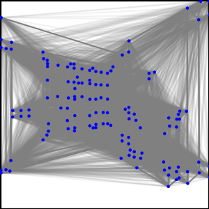
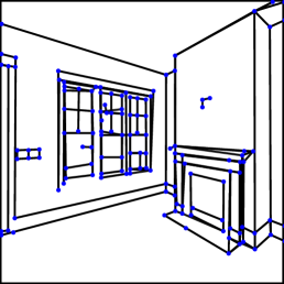
As illustrated in Fig. 1(b), the negative subset usually contains many hard negative samples since the proposed holistic AFM usually generates line segment proposals of “good quality”, which is helpful to learn a better verification classifier. Apart from the learned positive and negative samples, we use a simple proposal augmentation method in a similar spirit to the static sampler used in L-CNN [40]: We add all the groundtruth line segments into the positive set. We also introduce a set of negative samples that are generated based on the groundtruth junction annotations (i.e., line segments using the two end-points that do not correspond to any annotated line segment). During training, to avoid the class imbalance issue, we sample the same number, , of positives and negatives (i.e., LoIs) from the two augmented subsets ( in all our experiments). We use binary cross entropy loss in the verification module. Denote by the loss computed on the sampled LoIs.
The proposed HAWP is trained end-to-end with the following loss function,
| (3) |
5 Experiments
In this section, we present detailed experimental results and analyses of the proposed HAWP. Our reproducible PyTorch source code will be released.
Benchmarks. The wireframe benchmark [14] and the YorkUrban benchmark are used. The former consists of training samples and testing samples. The latter includes samples in total. The model is only trained on the former and tested on both.
Baselines. Four methods are used: LSD [29]111The built-in LSD in OpenCV v3.2.0 is used in evaluation., AFM [33], DWP [14], and L-CNN [40] (the previous state-of-the-art approach). The last three are DNN based approaches and the first one does not need training. The last two leverage junction information in training, and thus are directly comparable to the proposed HAWP.
Implementation Details. To be fair in comparison with L-CNN, we adopt the same hyper-parameter settings (including those defined in Section 4) when applicable in our HAWP. Input images are resized to in both training and testing. For the stacked Hourglass feature backbone, the number of stacks, the depth of each Hourglass module and the number of blocks are 2, 4, 1 respectively. Our HAWP is trained using the ADAM optimizer [15] with a total of epochs on a single Tesla V100 GPU device. The learning rate, weight decay rate and batch size are set to , and respectively. The learning rate is divided by at the -th epoch. To further ensure apple-to-apple comparisons with L-CNN, we also re-train it using the same learning settings with slightly better performance obtained than those reported in their paper.
| Method | Wireframe Dataset | YorkUrban Dataset | FPS | ||||||||||||
| sAP5 | sAP10 | sAP15 | msAP | mAPJ | APH | FH | sAP5 | sAP10 | sAP15 | msAP | mAPJ | APH | FH | ||
| LSD [29] | / | / | / | / | / | 55.2 | 62.5 | / | / | / | / | / | 50.9 | 60.1 | 49.6 |
| AFM [33] | 18.5 | 24.4 | 27.5 | 23.5 | 23.3 | 69.2 | 77.2 | 7.3 | 9.4 | 11.1 | 9.3 | 12.4 | 48.2 | 63.3 | 13.5 |
| DWP [14] | 3.7 | 5.1 | 5.9 | 4.9 | 40.9 | 67.8 | 72.2 | 1.5 | 2.1 | 2.6 | 2.1 | 13.4 | 51.0 | 61.6 | 2.24 |
| L-CNN [40] | 58.9 | 62.9 | 64.9 | 62.2 | 59.3 | 80.3 | 76.9 | 24.3 | 26.4 | 27.5 | 26.1 | 30.4 | 58.5 | 61.8 | 15.6 |
| 82.8† | 81.3† | 59.6† | 65.3† | ||||||||||||
| L-CNN (re-trained) | 59.7 | 63.6 | 65.3 | 62.9 | 60.2 | 81.6 | 77.9 | 25.0 | 27.1 | 28.3 | 26.8 | 31.5 | 58.3 | 62.2 | 15.6 |
| 83.7† | 81.7† | 59.3† | 65.2† | ||||||||||||
| HAWP (ours) | 62.5 | 66.5 | 68.2 | 65.7 | 60.2 | 84.5 | 80.3 | 26.1 | 28.5 | 29.7 | 28.1 | 31.6 | 60.6 | 64.8 | 29.5 |
| 86.1† | 83.1† | 61.2† | 66.3† | ||||||||||||
5.1 Evaluation Metric
We follow the accuracy evaluation settings used in L-CNN summarized as follows to be self-contained.
Structural Average Precision (sAP) of Line Segments [40]. This is motivated by the typical AP metric used in evaluating object detection systems. A counterpart of the Intersection-over-Union (IoU) overlap is used. For each ground-truth line segment , we first find the set of parsed line segments each of which, , satisfies the “overlap”,
| (4) |
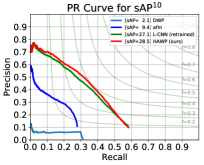
where or , and is a predefined threshold. If the set of parsed line segments “overlapping” with is empty, the line segment is counted as a False Negative (FN). If there are multiple candidates in the set, the one with the highest verification classification score is counted as a True Positive (TP), and the rest ones will be counted as False Positives (FPs). A parsed line segment that does not belong to the candidate set of any groundtruth line segment is also counted as a FP. Then, sAP can be computed. To eliminate the influence of image resolution, the wireframe parsing results and the groundtruth wireframes are rescaled to the resolution of in evaluation. We set the threshold to and report the corresponding results, denoted by sAP5, sAP10, sAP15. The overall performance of a wireframe parser is represented by the mean of the sAP values with different thresholds, denoted by msAP.
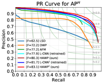
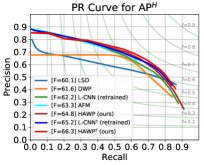
Heatmap based F-score, FH and APH of Line Segments. These are traditional metrics used in LSD and wireframe parsing [14]. Instead of directly using the vectorized representation of line segments, heatmaps are used, which are generated by rasterizing line segments for both parsing results and the groundtruth. The pixel-level evaluation is used in calculating the precision and recall curves with which FH and APH are computed.
Vectorized Junction Mean AP (mAPJ) [40]. It is computed in a similar spirit to msAP of line segments. Let be the thresold for the distance between a predicted junction and a groundtruth one. The mAPJ is computed w.r.t. .
LSD


DWP

AFM


L-CNN

HAWP (ours)

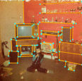
Ground Truth
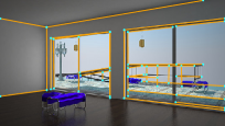

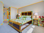
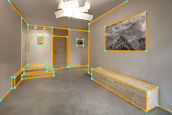
Speed. Besides accuracy, speed is also important in practice. We use the frames per second (FPS) in evaluation. For fair comparisons, we compute the FPS for different methods under the same setting: the batch-size is , and single CPU thread and single GPU (Tesla V100) are used. Note that the LSD [29] method does not take advantage of GPU.
5.2 Results and Comparisons
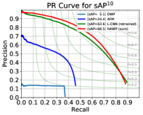
Quantitative Results. Table 1 summarizes the results and comparisons in terms of the evaluation metric stated in Section 5.1. Our HAWP obtains state-of-the-art performance consistently. In terms of the challenging msAP metric, it outperforms L-CNN by 2.8% and 1.3% (absolute improvement) on the wireframe benchmark and the YorkUrban benchmark respectively. It also runs much faster than L-CNN with 89% relative improvement in FPS. AFM and DWP are relatively slow due to their non-GPU friendly post-processing modules entailed for performance. In terms of the heatmap based evaluation metric, our HAWP is also significantly better than L-CNN regardless of the post-processing module proposed in L-CNN. Fig. 4 shows comparisons of PR curves.
Since our proposed HAWP and L-CNN use very similar wireframe parsing pipelines and adopt the same design choices when applicable. The consistent accuracy gain of our HAWP must be contributed by the novel 4-D holistic attraction field representation and its integration in the parsing pipeline. In terms of efficiency, our HAWP runs much faster since a significantly fewer number of line segment proposals are used in the verification module. As shown in Table 2, our HAWP uses 5.5 times fewer number of line segment proposals.
| # Junctions | # Proposals | sAP10 | FPS | # GT Lines | |
| L-CNN [40] | 159.2 | 22k | 63.6 | 15.6 | 74.2 |
| HAWP (ours) | 189.6 | 4k | 66.5 | 29.5 |
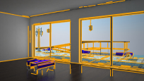
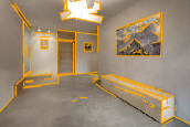
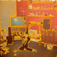
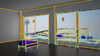
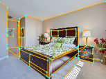
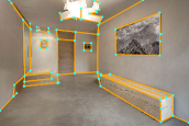
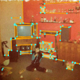
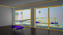
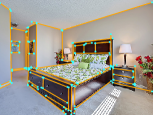
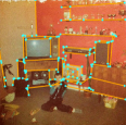
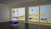
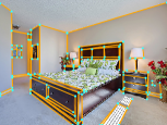
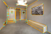
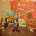
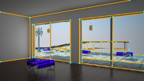
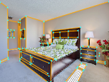
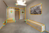
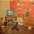
Qualitative Results. Fig. 5 shows wireframe parsing results by the five methods.
5.3 Ablation Study
We compare the effects of three aspects: our proposed H-AFM vs. the vanilla AFM [33], the distance residual module (Section 4.1), and the composition of negative samples in training verification module (Section 4.4).
| Line Segment Representation | Distance Residual | Negative Example Sampler | Performance | ||||||
| Training | Testing | sAP5 | sAP10 | sAP15 | |||||
| H-AFM | ✓ | ✓ | ✓ | ✓ | 62.5 | 66.5 | 68.2 | ||
| ✓ | 62.0 | 66.0 | 67.6 | ||||||
| ✓ | ✓ | ✓ | 62.2 | 66.1 | 67.8 | ||||
| ✓ | ✓ | 62.0 | 65.8 | 67.4 | |||||
| H-AFM | ✓ | ✓ | ✓ | 58.9 | 63.0 | 64.8 | |||
| H-AFM | ✓ | ✓ | 58.7 | 62.6 | 64.4 | ||||
| AFM | ✓ | ✓ | 30.9 | 33.7 | 35.0 | ||||
Table 3 summarizes the comparisons. We observe that both H-AFM and the distance residual module are important for improving performance. The natural negative sampler randomly chooses negative line segments based on the matching results (with respect to the annotations). The rest of three negative example samplers () are also investigated in L-CNN and their full combination is needed for training L-CNN. randomly selects a part of examples from the online generated line segment proposals, regardless of the matching results. tries to match the proposals with pre-computed hard negative examples and the matched proposals are used as negative samples. directly obtains the negative examples from the pre-computed hard negative examples set. In our experiment, the number of samples for and are set to respectively. We observe that our HAWP is less sensitive to those samplers due to the informative line segment proposal generation stage.
6 Conclusions and Discussions
This paper presents a holistically-attracted wireframe parser (HAWP) with state-of-the-art performance obtained on two benchmarks, the wireframe dataset and the YorkUrban dataset. The proposed HAWP consists of three components: proposal (line segments and junctions) initialization, proposal refinement and proposal verification, which are end-to-end trainable. Compared to the previous state-of-the-art wireframe parser L-CNN [40], our HAWP is enabled by a novel 4-D holistic attraction field map representation (H-AFM) for line segments in proposal generation stages. Our HAWP also achieves real-time speed with a single GPU, and thus is useful for many downstream tasks such as SLAM and Structure from Motion (SfM). The proposed H-AFM is also potentially useful for generic LSD problems in other domains such as medical image analysis.
References
- [1] Cuneyt Akinlar and Cihan Topal. Edlines: A real-time line segment detector with a false detection control. Pattern Recognition Letters, 32(13):1633–1642, 2011.
- [2] Emilio J Almazan, Ron Tal, Yiming Qian, and James H Elder. MCMLSD: A Dynamic Programming Approach to Line Segment Detection. In IEEE Conference on Computer Vision and Pattern Recognition (CVPR), 2017.
- [3] Dana H. Ballard. Generalizing the hough transform to detect arbitrary shapes. Pattern Recognition, 13(2):111–122, 1981.
- [4] Adrien Bartoli and Peter F. Sturm. Structure-from-motion using lines: Representation, triangulation, and bundle adjustment. Computer Vision and Image Understanding, 100(3):416–441, 2005.
- [5] J. Brian Burns, Allen R. Hanson, and Edward M. Riseman. Extracting straight lines. IEEE Trans. Pattern Analysis and Machine Intelligence, 8(4):425–455, 1986.
- [6] Rui Chen, Songfang Han, Jing Xu, and Hao Su. Point-based multi-view stereo network. In IEEE International Conference on Computer Vision (ICCV), 2019.
- [7] Nam Gyu Cho, Alan Yuille, and Seong Whan Lee. A Novel Linelet-Based Representation for Line Segment Detection. IEEE Trans. Pattern Analysis and Machine Intelligence, 40(5):1195–1208, 2018.
- [8] Patrick Denis, James H. Elder, and Francisco J. Estrada. Efficient Edge-Based Methods for Estimating Manhattan Frames in Urban Imagery. In European Conference on Computer Vision (ECCV), pages 197–210, 2008.
- [9] Agnès Desolneux, Lionel Moisan, and Jean-Michel Morel. Meaningful alignments. International Journal of Computer Vision, 40(1):7–23, 2000.
- [10] Timothy Duff, Kathlen Kohn, Anton Leykin, and Tomas Pajdla. Plmp - point-line minimal problems in complete multi-view visibility. In IEEE International Conference on Computer Vision (ICCV), October 2019.
- [11] Ross B. Girshick. Fast R-CNN. In IEEE International Conference on Computer Vision (ICCV), pages 1440–1448, 2015.
- [12] Abhinav Gupta, Alexei A. Efros, and Martial Hebert. Blocks world revisited: Image understanding using qualitative geometry and mechanics. In European Conference on Computer Vision (ECCV), pages 482–496, 2010.
- [13] Kaiming He, Georgia Gkioxari, Piotr Dollár, and Ross B. Girshick. Mask R-CNN. In IEEE International Conference on Computer Vision (ICCV), pages 2980–2988, 2017.
- [14] Kun Huang, Yifan Wang, Zihan Zhou, Tianjiao Ding, Shenghua Gao, and Yi Ma. Learning to parse wireframes in images of man-made environments. In IEEE Conference on Computer Vision and Pattern Recognition (CVPR), pages 626–635, 2018.
- [15] Diederik P. Kingma and Jimmy Ba. Adam: A method for stochastic optimization. In International Conference on Learning Representations (ICLR), 2015.
- [16] Pierre-Alain Langlois, Alexandre Boulch, and Renaud Marlet. Surface reconstruction from 3d line segments. In International Conference on 3D Vision (3DV), pages 553–563, 2019.
- [17] Hei Law and Jia Deng. Cornernet: Detecting objects as paired keypoints. In European Conference on Computer Vision (ECCV), pages 765–781, 2018.
- [18] Thomas Lemaire and Simon Lacroix. Monocular-vision based SLAM using line segments. In IEEE International Conference on Robotics and Automation (ICRA). IEEE, apr 2007.
- [19] Kevis-Kokitsi Maninis, Jordi Pont-Tuset, Pablo Arbelaez, and Luc Van Gool. Convolutional oriented boundaries: From image segmentation to high-level tasks. IEEE Trans. Pattern Analysis and Machine Intelligence, 40(4):819–833, 2018.
- [20] Jiri Matas, Charles Galambos, and Josef Kittler. Robust detection of lines using the progressive probabilistic hough transform. Computer Vision and Image Understanding, 78(1):119–137, 2000.
- [21] Branislav Micusík and Horst Wildenauer. Structure from motion with line segments under relaxed endpoint constraints. International Journal of Computer Vision, 124(1):65–79, 2017.
- [22] Alejandro Newell, Kaiyu Yang, and Jia Deng. Stacked hourglass networks for human pose estimation. In European Conference on Computer Vision (ECCV), pages 483–499, 2016.
- [23] Bronislav Pribyl, Pavel Zemcík, and Martin Cadík. Camera pose estimation from lines using plücker coordinates. In Proceedings of the British Machine Vision Conference 2015, BMVC, pages 45.1–45.12, 2015.
- [24] Bronislav Pribyl, Pavel Zemcík, and Martin Cadík. Absolute pose estimation from line correspondences using direct linear transformation. Computer Vision and Image Understanding, 161:130–144, 2017.
- [25] Shaoqing Ren, Kaiming He, Ross B. Girshick, and Jian Sun. Faster R-CNN: towards real-time object detection with region proposal networks. IEEE Trans. Pattern Analysis and Machine Intelligence, 39(6):1137–1149, 2017.
- [26] Lawrence G Roberts. Machine perception of three-dimensional solids. PhD thesis, Massachusetts Institute of Technology, 1963.
- [27] Zhuowen Tu, Xiangrong Chen, Alan L. Yuille, and Song Chun Zhu. Image parsing: Unifying segmentation, detection, and recognition. International Journal of Computer Vision, 63(2):113–140, 2005.
- [28] Gül Varol, Duygu Ceylan, Bryan C. Russell, Jimei Yang, Ersin Yumer, Ivan Laptev, and Cordelia Schmid. Bodynet: Volumetric inference of 3d human body shapes. In European Conference on Computer Vision (ECCV), pages 20–38, 2018.
- [29] R G von Gioi, J Jakubowicz, J M Morel, and G Randall. LSD: A Fast Line Segment Detector with a False Detection Control. IEEE Trans. Pattern Analysis and Machine Intelligence, 32(4):722–732, 2010.
- [30] Shih-En Wei, Varun Ramakrishna, Takeo Kanade, and Yaser Sheikh. Convolutional pose machines. In IEEE Conference on Computer Vision and Pattern Recognition (CVPR), pages 4724–4732, 2016.
- [31] Gui-Song Xia, Julie Delon, and Yann Gousseau. Accurate junction detection and characterization in natural images. International Journal of Computer Vision, 106(1):31–56, 2014.
- [32] Saining Xie and Zhuowen Tu. Holistically-nested edge detection. International Journal of Computer Vision, 125(1-3):3–18, 2017.
- [33] Nan Xue, Song Bai, Fudong Wang, Gui-Song Xia, Tianfu Wu, and Liangpei Zhang. Learning attraction field representation for robust line segment detection. In IEEE Conference on Computer Vision and Pattern Recognition (CVPR), 2019.
- [34] Nan Xue, Song Bai, Fudong Wang, Gui-Song Xia, Tianfu Wu, Liangpei Zhang, and Philip H.S. Torr. Learning regional attraction for line segment detection. IEEE Trans. Pattern Analysis and Machine Intelligence, 2019.
- [35] Nan Xue, Gui-Song Xia, Xiang Bai, Liangpei Zhang, and Weiming Shen. Anisotropic-scale junction detection and matching for indoor images. IEEE Trans. Image Processing, 2018.
- [36] Zhucun Xue, Nan Xue, Gui-Song Xia, and Weiming Shen. Learning to calibrate straight lines for fisheye image rectification. In IEEE Conference on Computer Vision and Pattern Recognition (CVPR), 2019.
- [37] Ziheng Zhang, Zhengxin Li, Ning Bi, Jia Zheng, Jinlei Wang, Kun Huang, Weixin Luo, Yanyu Xu, and Shenghua Gao. Ppgnet: Learning point-pair graph for line segment detection. In IEEE Conference on Computer Vision and Pattern Recognition (CVPR), 2019.
- [38] Huizhong Zhou, Danping Zou, Ling Pei, Rendong Ying, Peilin Liu, and Wenxian Yu. Structslam: Visual SLAM with building structure lines. IEEE Trans. Vehicular Technology, 64(4):1364–1375, 2015.
- [39] Xiaowei Zhou, Menglong Zhu, Georgios Pavlakos, Spyridon Leonardos, Konstantinos G. Derpanis, and Kostas Daniilidis. Monocap: Monocular human motion capture using a CNN coupled with a geometric prior. IEEE Trans. Pattern Anal. Mach. Intell., 41(4):901–914, 2019.
- [40] Yichao Zhou, Haozhi Qi, and Yi Ma. End-to-end wireframe parsing. In IEEE International Conference on Computer Vision (ICCV), 2019.
- [41] Xingxing Zuo, Xiaojia Xie, Yong Liu, and Guoquan Huang. Robust visual SLAM with point and line features. In IEEE/RSJ International Conference on Intelligent Robots and Systems (IROS). IEEE, 2017.