Sympatric speciation based on pure assortative mating

Abstract

Although geographic isolation has been shown to play a key role in promoting reproductive isolation, it is now believed that speciation can also happen in sympatry and with considerable gene flow. Here we present a model of sympatric speciation based on assortative mating that does not require a genetic threshold for reproduction, i.e., that does not directly associate genetic differences between individuals with reproductive incompatibilities. In the model individuals mate with the most similar partner in their pool of potential mates, irrespective of how dissimilar it might be. We show that assortativity alone can lead to the formation of clusters of genetically similar individuals. The absence of a minimal genetic similarity for mating implies the constant generation of hybrids and brings up the old problem of species definition. Here, we define species based on clustering of genetically similar individuals but allowing genetic flow among different species. We show that the results obtained with the present model are in good agreement with empirical data, in which different species can still reproduce and generate hybrids.

Keywords: evolution, species definition, hybrids, genetic flow

1 Introduction

One of the main goals of evolutionary biology is to uncover the processes responsible for the origin and maintenance of biodiversity. However, the very concept of species has been the subject of an endless discussion in evolutionary theory [1, 2, 3, 4, 5, 6, 7, 8, 9, 10]. While useful from a theoretical point of view, the famous Biological Species Concept (BSC), based on reproductive isolation, is very hard to test in practice and cannot deal adequately with hybridizations [11]. According to the BSC, a species is a group of organisms that can reproduce with one another and that are reproductively isolated from other such groups. When the mating pattern of the individuals is assortative, i.e., when mating occurs preferentially between individuals with similar phenotypes, the gene flow between species is limited, helping to keep them separated [12, 13]. However, individuals from different species do eventually mate and produce viable offspring, posing a challenge to the BSC definition. This is the case of the butterfly Heliconius cydno cydnides and Heliconius cydno weymeri that live in sympatry (same geographic area) in the Cauca Valley (Colombia). It has been shown that Heliconius cydno cydnides males court and produce viable offsprings with Heliconius cydno cydnides and Heliconius cydno weymeri females, but they have a strong preference for females of the same species [14]. Perhaps the most celebrated case of in which mating is assortative but interbreeding produces fertile hybrids is the cichlid fish in the African lakes [15]. Lakes Malawi and Victoria, in particular, exhibit an exuberant fauna of haplochromine cichlids. There are convincing evidences of female choice based on male coloration in both artificial conditions and natural environments [16]. Nevertheless, under certain conditions, such as inappropriate lighting environment, mate choice becomes random and viable offspring are produced [17]. Assortative mating is believed to be the main genetic barrier between the butterfly species and it is also invoked to explain the explosive radiation of cichlid fish in African lakes [15].

The incorporation of assortativity in speciation models is a way to understand the dynamics of speciation in systems such as Heliconius and African cichlid fish, where species have possibly diversified in sympatry with assortment playing an important role as a source of reproductive isolation [18, 19, 20]. Models with assortative mating can be distinguished between one- and two-trait models [21, 22]. These two kinds of models differ on whether the set of loci under viability selection and the loci involved in assortative mating are the same or not [23]. Selectively neutral one-trait models have been shown not to lead to speciation due to the stabilization of the sexual selection generated by assortative mating [24, 25, 26]. The combination of selection and assortativeness, however, can be very effective at eliminating intermediary genotypes, resulting in sympatric speciation [27, 28]. Alternatively, assortative mating combined with spatial structure and mating with nearby individuals can also lead to the formation of local groups of similar individuals that eventually break into species [29, 30, 31, 32]. Two-trait models, which separate the trait under selection – such as body size or eye color – and the trait under assortative mating, have showed that, if linkage is tight and assortment is strong, reproductive isolation can emerge [33, 34].

An important model of assortative mating was proposed by Derrida and Higgs (DH) [35], which demonstrated the possibility of speciation in sympatric populations involving no other selective forces or spatial structure. One key aspect of the model is the approximation of infinitely large genomes [36]. In this model assortative mating is controlled by a measure of genetic similarity between individuals. An incompatibility threshold $q_{min}$ is introduced in such a way that reproduction becomes impossible between individuals $i$ and $j$ whose similarity $q_{ij}$ is smaller than $q_{min}$. The incompatibility threshold allows the definition of species as groups of individuals reproductively isolated from those in different groups, similar to the BSC. This definition is very convenient for theoretical models and has been adopted by many authors [10, 37, 38, 39, 35, 36]. Given a similarity threshold $q_{min}$, it is easy to design an algorithm that separates the population into clusters in such way that individuals belonging to different clusters have genetic similarity smaller that $q_{min}$. Within clusters, on the other hand, individuals will have at least one partner whose genetic similarity is larger than $q_{min}$. The process is similar to finding components of a network where nodes (individuals) are connected only if their similarity is larger than $q_{min}$. However, in real cases of incipient speciation such threshold may not exist and the populations will not separate in perfectly isolated groups, as illustrated by Heliconius and African cichlid fish systems, in which different species can still reproduce and generate hybrids.

Here we propose a model of speciation based on pure assortativity, where no spatial structure or similarity threshold to reproduction are imposed. The evolutionary dynamics is based on the model by Derrida and Higgs [35], with the difference that individuals will mate with the most similar individual in their pool of potential partners, characterizing positive assortative mating, but with no restrictions imposed by a similarity threshold. We show that assortative mating alone can lead to the formation of groups of genetically similar individuals that will reproduce preferentially with others in the same group, but might occasionally choose individuals from other groups as mating partners, generating viable hybrids. One important feature of the model is that it brings back the discussion of species definition: the clusters that form are not reproductively isolated from each other and are constantly, though rarely, generating hybrids. This recovers the case of African cichlids and other incipient species where mate choice does not seem to be related to genetic incompatibilities. The model provides a good representation of speciation by assortative mating in a genetically neutral scenario.

2 Methods

2.1 Assortative Mating

Our model is a modification of the model proposed by Derrida and Higgs (DH) [35], in which a population of M haploid individuals evolves by sexual reproduction with a genetic threshold determining mating compatibility. Each individual is characterized by a genome represented by a binary sequence of size $B$, $\{S_{1}^{\alpha},S_{2}^{\alpha},\dots,S_{B}^{\alpha}\}$, where $S_{i}^{\alpha}$ is the $i^{th}$ gene of the individual $\alpha$ and can assume the values $\pm 1$. The population is characterized by a $M\times M$ matrix $Q$ measuring the degree of genetic similarity between pairs of individuals. The elements of $Q$ are given by:

$$q^{\alpha\beta}=\frac{1}{B}\sum_{i=1}^{B}S_{i}^{\alpha}S_{i}^{\beta}.$$ (1)

Genetically identical individuals have $q^{\alpha\beta}=1$ whereas individuals with randomly assigned genes have $q^{\alpha\beta}$ close to zero. Also, since every individual is identical to itself, $q^{\alpha\alpha}\equiv 1$ at all times. All results in this paper are obtained in the limit of infinitely large genomes, $B\rightarrow\infty$ as described below.

In the original DH model the population at each generation is obtained from the previous one by sexual reproduction of parents with a minimal genetic similarity threshold $q_{min}$, as follows: an individual is randomly chosen from the population to be the first parent, $P_{1}$. Then a second parent, $P_{2}$ is selected from the remaining $M-1$ individuals. If $P_{1}$ and $P_{2}$ are sufficiently similar, i.e., if $q^{P_{1},P_{2}}\geq q_{min}$ an offspring is produced by combining the genomes of the parents. If, however, $q^{P_{1},P_{2}}<q_{min}$, the pair is considered incompatible and another individual is randomly chosen for the role of $P_{2}$. If the similarity condition cannot be met by any member of the population, another first parent $P_{1}$ is chosen and the process repeated until a compatible mating pair is found. The genome of the offspring is inherited, gene by gene, from the parents’ genomes with equal probability. There is also a small probability, $\mu$, that a mutation occurs in each gene of the offspring. The entire process is repeated until $M$ offspring have been produced, forming the next generation.

The idea behind the hypothesis of a minimum similarity for mating is reminiscent of the Batenson-Dobzhansky-Muller model [40, 41, 42, 43] where alleles at different loci of diploid individuals might be incompatible. Here each difference between haploid genomes reduces the chances of producing a viable offspring by introducing some degree of incompatibility. As the number of differences increases the chances of a successful reproduction decreases. A simple way to deal with this idea is by assuming that individuals become totally incompatible if the number of genetic differences exceeds a threshold but are perfectly compatible below that value. However, such a sharp threshold is a simplification of the real mating dynamics as genetic incompatibilities might not exist at all, as in the case of cichlids [17].

In the present model the condition of minimum similarity for mating is completely removed. Instead, after a first parent $P_{1}$ has been randomly chosen, a pool $R$, with $N$ individuals is randomly selected from the remaining population: $R=\{R_{1},R_{2},\dots,R_{N}\}$. The second parent is now chosen from the pool as the individual with the highest degree of similarity with $P_{1}$. Thus, $P_{2}=R_{i}$, such that: $q^{P_{1}R_{i}}=max(q^{P_{1}R_{j}})$, with $j=1,2,\dots,N$. Mating is, therefore, purely assortative and relies on the power of the first parent to choose its mate from the pool, with no restriction regarding genetic distance. An offspring is always produced by combining the genomes of $P_{1}$ and $P_{2}$, no matter how different they might be. Like in the original DH model, parents’ genomes are combined gene by gene with a mutation rate $\mu$ per gene and the process is repeated until $M$ offspring have been generated.

The model we propose here can be interpreted as a type of best-of-n model [44, 45]. In this case, a female evaluates $n$ randomly selected males and chooses the one closest to her preferred phenotype . It has been show that best-of-n models may lead to speciation, however not in the neutral context as in the present work [46]

In order to get some insight on how the overlap matrix evolves through time, we follow DH and consider first the simplest case of asexual reproduction, in which each individual $\alpha$ has a single parent $P(\alpha)$. The allele $S_{i}^{\alpha}$ has probability $\frac{1}{2}(1+e^{-2\mu})$ of inheriting the allele $S_{i}^{P(\alpha)}$ without mutating and probability $\frac{1}{2}(1-e^{-2\mu})$ of undergoing a mutation and assuming the value $-S_{i}^{P(\alpha)}$. Under these conditions, the expected value of $q^{\alpha\beta}$ is:

$$E(q^{\alpha\beta})=e^{-4\mu}q^{P(\alpha)P(\beta)}$$ (2)

In the case of sexual reproduction the individuals $\alpha$ and $\beta$ have two parents each: $P_{1}(\alpha)$, $P_{2}(\alpha)$ and $P_{1}(\beta)$, $P_{2}(\beta)$, respectively. On average, half of the alleles are inherited from $P_{1}$ and the other half from $P_{2}$. Thus, the expected value of $q^{\alpha\beta}$ is:

$$E(q^{\alpha\beta})=\frac{e^{-4\mu}}{4}\left[q^{P_{1}(\alpha)P_{1}(\beta)}+q^{P_{2}(\alpha)P_{1}(\beta)}+q^{P_{1}(\alpha)P_{2}(\beta)}+q^{P_{2}(\alpha)P_{2}(\beta)}\right]$$ (3)

The above expressions are exact for infinitely large genomes ($B\rightarrow\infty$) and the dynamics of the population can be obtained by simply updating the similarity matrix. Therefore, given the population at generation $t$ and similarity matrix $Q$, the next generation is constructed by producing $M$ offspring with parents at generation $t$ as described above. Equation 3 is then used to update $Q$. If mating is not restricted by similarity and if the pool size is $N=1$, it can be shown that all elements $q^{\alpha\beta}$ of the similarity matrix converge to the value $q_{conv}\approx\frac{1}{(1+4\mu M)}$ [35]. The population will break into species if a threshold value $q_{min}>q_{conv}$ is introduced [35]. Here we show that the population still breaks into species if the minimum similarity requirement is eliminated but pool sizes for choosing the second parent are sufficiently large.

2.2 Species Definition

In the DH model of speciation two individuals $i$ and $j$ cannot reproduce if $q^{ij}<q_{min}$. This genetic compatibility threshold at the individual level can be extended to the species level to define reproductive isolation between groups of individuals, as in the biological species concept. In the DH model a species can be identified as a group of individuals reproductively isolated from all others outside the group by the genetic threshold $q_{min}$. Not all members of the group have to be able to mate with each other, but could maintain an indirect gene flow through an intermediary individual. Therefore, if $q^{ij}>q_{min}$ and $q^{jk}>q_{min}$ but $q^{ik}<q_{min}$, individuals $i$,$j$ and $k$ will belong to the same species, owing to the ongoing gene flow between them.

In the present model of pure assortative mating no such threshold exists and, as discussed before, the concept of species is fuzzy and relies on the identification of clusters of similar individuals. In order to do that we are going to define an auxiliary threshold value $q_{0}$ that will play the role of $q_{min}$ in our model for the sake of species definition. This value will be calculated at a specific generation, when the population dynamics reaches a state of equilibrium, and will be used to organize the population into species in all generations, before and after the moment of calculation. Our definition of $q_{0}$ will be based on the clustering method proposed in [47] and [48] which uses the eigenvalues of the unnormalized Laplacian matrix defined as

$$L=D-Q.$$ (4)

Here $Q$ is the similarity matrix whose elements are given by equation (1) and $D$ is the degree matrix, whose elements are given by:

$$d_{i,j}=\left\{\begin{array}[]{rc}0,&\mbox{if}\ i\neq j,\\ \sum_{k=1}^{M}q^{ik},&\mbox{if}\ i=j\end{array}\right.$$ (5)

One important property of $L$ is that for every vector $f\in\mathbb{R}^{N}$

$$f^{T}Lf=\frac{1}{2}\sum_{i,j=1}^{M}q^{ij}(f_{i}-f{j})^{2}.$$ (6)

If all elements $q^{ij}$ are positive, this would imply that $L$ has $M$ non-negative eigenvalues and that 0 is an eigenvalue associated with the constant eigenvector. Although the $q^{ij}$’s can be negative (for example if $S^{i}_{k}=1$ and $S^{j}_{k}=-1$ for all $k$, $q^{ij}=-1$) they are always positive in the simulations, as we start with $q^{ij}=1$ and evolution keeps them positive at all times. Thus, it is possible to establish the following proposition: if $k$ is the multiplicity of the eigenvalue 0 of $L$, then the graph represented by $Q$ has $k$ disconnected components [48]. Based on these properties we propose the following procedure to determine $q_{0}$: we define a new similarity matrix $Q(s)$ whose elements are given by:

$$q^{ij}(s)=\left\{\begin{array}[]{rc}0,&\mbox{if}\ q^{ij}<s\\ q^{ij},&\mbox{if}\ q^{ij}>s\end{array}\right..$$ (7)

In terms of graph theory this is equivalent to consider vertices with connection smaller than $s$ to be disconnected. From $Q(s)$ one obtains $D(s)$ and $L(s)$. Therefore, following the number $k$ of eigenvalues 0 (the multiplicity of the eigenvalue 0) as a function of $s$, it is possible to find an appropriate value of this parameter that breaks the population into reasonably disconnected clusters and use this value as the definition of $q_{0}$. In other words, a cluster is defined as a group of individuals (vertices) that have larger genetic similarity among themselves than with individuals belonged to other clusters. Thus, the critical value $q_{0}$ is the lowest connection between vertices belonging to the same clusters. Disconnecting vertices with similarity larger than $q_{0}$ would produce a large number to totally disconnected individuals, causing the number of clusters to increase rapidly with $s$.

Figure 1: (upper panel) Number of eigenvalues $k(s)$ smaller than 10 for a population of $M=2000$, pool size $N=100$, after 10000 generations. (bottom panel) Magnification of the region around $s=0.95$. The inset shows the derivative $dk/ds$.

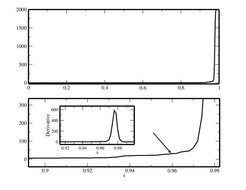
As an example, consider the hypothetical case of a population with $M$ individuals that is clearly split into two groups. Suppose the first group has $M_{1}$ individuals and that the minimum similarity between all its pairs is equal to $s_{1}$; the second group, with $M_{2}$ individuals, has minimum similarity between its pairs equal to $s_{2}$. We further assume that the minimum similarity between individuals belonging to different groups is $s_{3}$. Clearly $s_{3}<s_{1}$ and $s_{3}<s_{2}$ and, without losing generality, we assume $s_{2}<s_{1}$. In this case the behavior of $k(s)$ is as follows: For $0\leq s\leq s_{3}$, $k(s)=1$ since all pairs have similarity larger than $s_{3}$. For $s_{3}<s<s_{2}$, $k(s)=2$, the two groups were disconnected and the multiplicity of the eigenvalue zero is 2. Finally, for $s_{2}<s<s_{1},$ individuals belonging to the second cluster gradually become disconnected from the cluster and $k$ starts to increase continuously. We may thus consider that $q_{0}=s_{2}$ is the appropriate value of s that splits the population into components without fragmenting it into tiny clusters with few individuals each. The value, although still subjected to a degree of uncertainty, can be identified by the presence of a plateau in the plot of $k(s)$, before a sharp increase. It is important to stress that, different from the BSC, $q_{0}$ does not play a role in mating. In the present model, it is only a convenient parameter to define species. However, the strength of the present model is the possibility of mating between individuals with genetic similarity smaller than $q_{0}$.

One representative example from our simulations is shown in Figure 1 where we analyzed a population with 2000 individuals with pool size of 100 at the 10000-th generation. In this case the eigenvalues of the Laplacian matrix range typically from 0 to 3000 and we counted as $k(s)$, or ”close to zero”, those below 10. The upper panel of Figure 1 shows $k(s)$ and the bottom panel shows a zoom around $s=0.96$ with the derivative $dk/ds$ in the inset. From this figure we defined $q_{0}=0.96$ and use it as a criterion to define species. We acknowledge that there is a degree of subjectivity in this procedure. Different choices of $s$ would change the counting of species, but not the clustering itself.

3 Results

In this section we show results for a population with $M=2000$ individuals and $\mu=1/8000$. The simulation starts with all individuals genetically identical ($q^{\alpha\beta}=1$ for all $\alpha$ and $\beta$) and the expected equilibrium value of the similarity for the case of unit pool ($N=1$) is $q_{conv}=1/2$.

3.1 Species and similarities

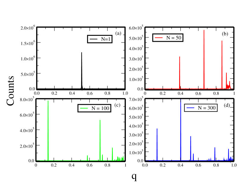
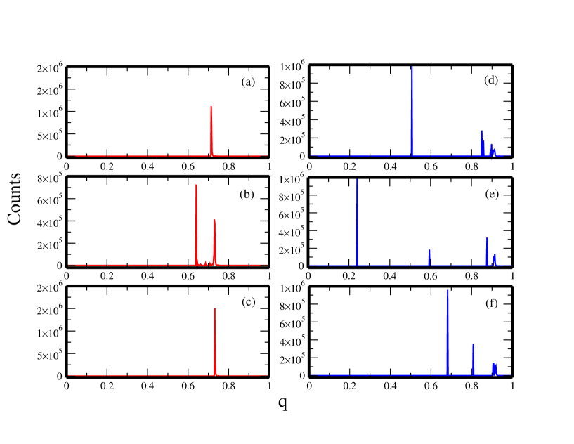
Figure 2a shows the histogram of $q^{\alpha\beta}$ between all pairs of individuals after 4000 generations for random mating ($N=1$) displaying the peak at $q=0.5$ as expected. Figures 2 b,c and d show similar results for pool sizes $N=50$, $100$ and $N=300$ respectively. The histograms exhibit peaks at large values of $q$, such as between 0.9 and 1.0, indicating that there are clusters of individuals with more than $90\%$ of genetic similarity. The peaks at lower values of $q$, on the other hand, correspond of pairs of individuals in different clusters, which is a signature of speciation. Figure 3 shows results for small pools of sizes 10 and 30.

Figure 2: Distribution of non-diagonal elements of the similarity matrix for a population of $M=2000$ individuals and pool sizes (a) 1; (b) 50; (c) 100 and (d) 300 at the generation $T=4000$. Panel (a) is the special case in which our model recovers the DH model. In all cases we have used $\mu=1/8000$.

Figure 3: Distribution of non-diagonal elements of the similarity matrix of a population of $M=2000$ individuals for pool sizes 10 (red, left panel) and 30 (blue, right panel). In both cases $\mu=1/8000$. From top to bottom the times are 4000, 5500 and 6000.

Figure 4: Time evolution of the distribution of non-diagonal elements of the similarity matrix for pool size $N=100$ and times 4000, 4100, 4200 and 4300.

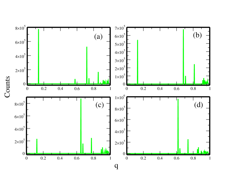
Similarly to the DH model [35] the peaks move to the left as time increases because of genetic drift and eventually disappear as species go extinct by fluctuation in the number of individuals. Figure 4 shows histograms of $q^{\alpha\beta}$ for $N=100$ at the generations 4000 (Figure 4a), 4100 (Figure 4b), 4200 (Figure 4c) and 4300 (Figure 4d). The peak close to $q=0.1$, for instance, moves slowly to left with decreasing amplitude, until it disappears completely (Figure 4d).

3.2 Number of species

Figures 5 a,b,c and d show the number of species as a function of time for pool size equal 1, 50, 100 and 300 individuals, respectively. For each pool size the value of $q_{0}$ is calculated. For small pool size ($N=1$, $q_{0}=0.504$, Figure 5a) there is only one species. This case, where the choice of mates is completely random, is the same case studied in [35] where no minimal genetic similarity threshold is imposed and, as it was anticipated, the number of species is one along the time and the diversity within the specie is very high ($q_{0}\sim 0.5$). Nevertheless, once the formation of pair is not completely random, one can see the emergence of new species as shown in Figures 5 b,c and d for $N=50$ with $q_{0}=0.938$, $N=100$ with $q_{0}=0.96$ and $N=300$ with $q_{0}=0.966$, respectively.

Figure 5: Time evolution of the number of species as a function of pool size for a population of $2000$ individuals and $\mu=1/8000$ for pool size equal to: (a) $N=1$, $q_{0}=0.504$, (b) $N=50$, $q_{0}=0.938$, (c) $N=100$, $q_{0}=0.96$ and (d) $N=300$, $q_{0}=0.966$.

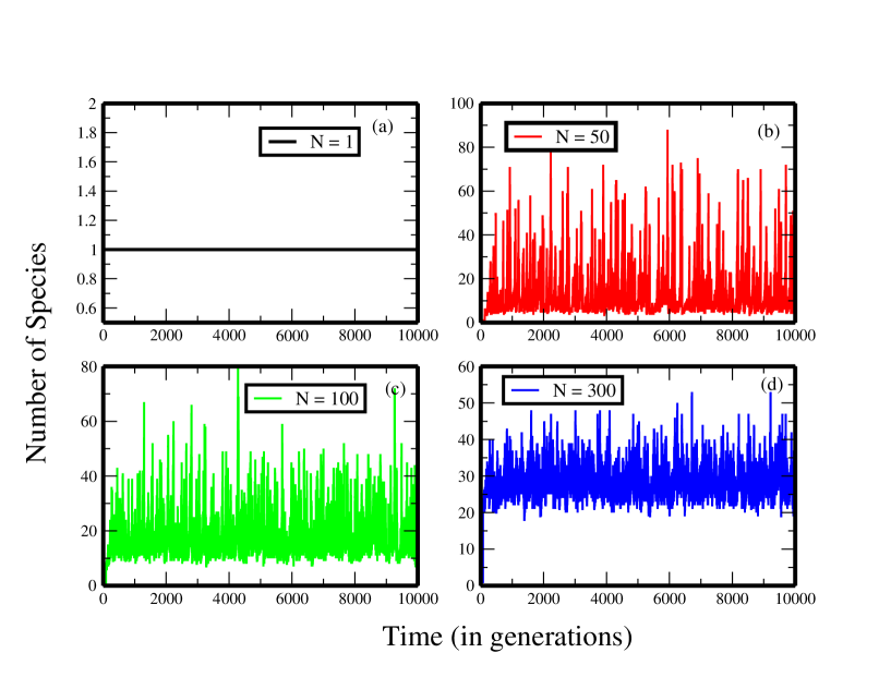
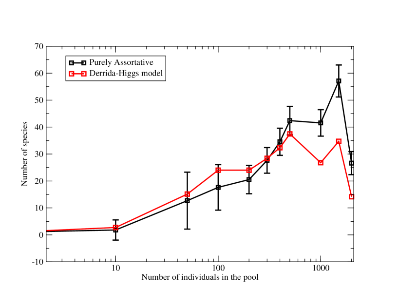
Figure 6 shows the time average and mean square deviation of the number of species for different values of the pool size $N$ (black line) compared with the expected number of species according to the DH model (red line). For each value of $N$ the parameter $q_{0}$ was calculated as indicated above. The number of species shown is the average computed from the same time series at every generation, from the initial time to 10,000. In the DH model the number of species can be estimated by supposing that the population has $n$ species with, on average $m$ individuals, so that $nm=M$. Using the fact that the mean value of the similarity of the group with $m$ individuals drifts to the value $q(m)=1/(1+4\mu m)$ and, imposing $q(m)=q_{0}$, we get $n=4\mu M(q_{0}^{-1}+1)^{-1}$.

Figure 6: Numerical average number of species as a function of the pool size in a purely assortative reproduction is considered (black) and analytical average number of species for the DH model (red) for $M=2000$. Black dots represent average values computed at every generation and vertical bars are mean square deviations. The values of $q_{0}$ for $N=1$, 10, 100 and 500 are 0.504, 0.732, 0.960 and 0.974 respectively.

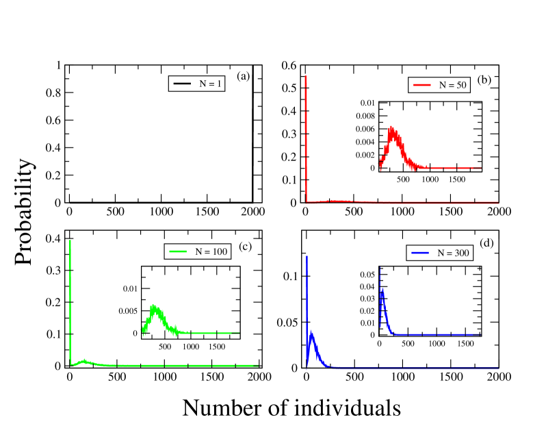
Finally, one important feature of a species is how many individuals it contains and how its size depends on $N$, the number of individuals in the pool. Clearly, as the number of species varies considerably, one could expect the same behavior for the number of individuals belonging to a certain species. Thus, a useful quantity to measure this is the abundance, which has a probability interpretation. The abundance is calculated as follows: after a specific transient time (we chose it as the generation 3000), the number of individuals in each species is recorded for every generation. At the end of the simulation (10000 generations), we construct a normalized histogram of the number of occurrence of species with a given number of individuals. Figures 7 a,b,c and d show the abundance for $N=1$, $N=50$, $N=100$ and $N=300$, respectively. $N=1$, shown in Figure 7a, is the trivial case in which there is only one species (see Figures 5a and 6a) and this species contains all individuals. On the other hand, as the pool size increases, a more complex probability distribution takes place. For example, in Figure 7b one can see a high probability of finding species with very few (or even with one individuals) but a finite, although very low, probability of finding species with a considerable number of elements. The peak at $1$ means that most of the individuals in the population are less similar than the threshold $q_{0}$ to all the others (see also Figures 8 and 9 below). For $N=100$, Figure 7c, the probability of finding abundant species with around 150 individuals, is already significant. Figure 5d shows the case where the pool size is a substantial fraction of the system. In such situation, although there exist species with only few elements, it is much more likely to find robust species with a great number of individuals.

Figure 7: Abundance of a population with 2000 individuals after 10000 generations for pool sizes equal to a) 1, b) 50, c) 100 and d) 300 individuals. The abundance was calculated from the generations 3000 and 10000 in order to avoid the spurious effects of the transient time. The insets show a zoom of the distribution for large abundances.

3.3 Hybridization

An interesting situation that can be well described by our model is that of hybridization of two species. In [49] the authors reported the evolution of two species of swordtail (Xiphophorus birchmanni and Xiphophorus malinche) that maintain their reproductive isolation in sympatry because of assortative mating. Nevertheless, a disruption of pheromonal communication due to pollution lead to a breakdown of assortativeness [50] and to the formation of a hybrid population that have persisted for over 25 generations.

In order to show that the model can capture the essence of this process we simulated a population with two species (A and B). Within each species, the individuals are initially genetically identical and the genetic similarity between individuals belonging to different species was set to $0.9$. We simulated the evolution to the next generation without assortativity (mimicking the effect of the pollution), allowing completely random mating (pool size equal 1). In the next generation assortativity was restored with pool size of 400 individuals, simulating the recovery of the ecological integrity of the environment. Figure 8 shows the time evolution of the number of species using $q_{0}=0.97$ for species definition.

In order to compare the results of simulations with empirical observations we counted as species only groups with more than 10 individuals. The red line in Figure 8 shows the number of species along the time when the population evolves according to our model. The black line shows the time evolution according to the Derrida-Higgs dynamics. Since DH-model does not allow hybridization, the two initial groups are preserved and no new species appear during this initial stage of the dynamics. On the other hand, after a hybridization period (of around 7 generations), a new hybrid species appears which persists for about 20 generations.

Figure 8: Time evolution of the number of species for the case where the assortativeness is broken at the first generation calculated by using our model (red line) and D.H. model (black line). After the first generation, the pool size is 400 individuals and the genetical similarity used to define specie is $q=0.97$. This $q$ is also used as genetic threshold in the D.H. model.

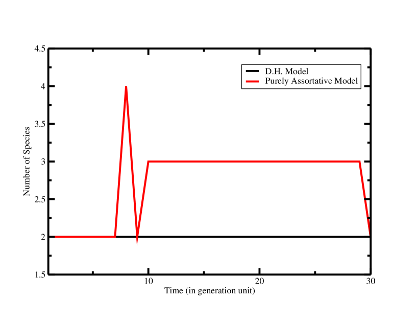
The results of Figure 8 can be understood as follows: at generation 1 the population breaks into three groups. Two of those groups, $A_{1}$ and $B_{1}$ are ‘pure’, meaning that their individuals are offspring of parents belonging to the same species, either A or B. Each of these groups has about $N/4$ individuals. The third group, $H_{1}$, with about $N/2$ individuals, contains the hybrids. The average genetic similarity between individuals belonging to $A_{1}$ (or $B_{1}$) is $q=e^{-4\mu}$ . The similarity between an individual in $A_{1}$ and one in $B_{1}$, on the other hand, is $q=0.9e^{-4\mu}$. Within the hybrid group $H_{1}$, or between $H_{1}$ and $A_{1}$ or $B_{1}$, the genetic similarity is $q=0.95e^{-4\mu}$. If we set $q_{0}$ to any value below $0.95e^{-4\mu}$ these three groups would be identified as a single species, since individuals of $H_{1}$ would be able to mate with both $A_{1}$ and $B_{1}$, establishing gene flow among all individuals of the population. In order to identify $A_{1}$ and $B_{1}$ as different species we need to set $q_{0}$ above $0.9e^{-4\mu}$ and we fixed $q_{0}=0.97$. In this case only $A_{1}$ and $B_{1}$ are well defined species whereas the hybrid group $H_{1}$ forms a cluster whose individuals can still mate with any other if there is no mating threshold, but are too different from each other to be considered a species. The abundance distribution of the population would be similar to Figure 7(b), with a peak at 1. This is illustrated in Figure 9a. For the model with mating threshold at $0.97$ they will all die without living offspring and the population will maintain its two species for many generations as shown in Figure 8.

Figure 9: Illustrative scheme for the first (a), second (b) and third (c) generation of the population evolving according with our model.

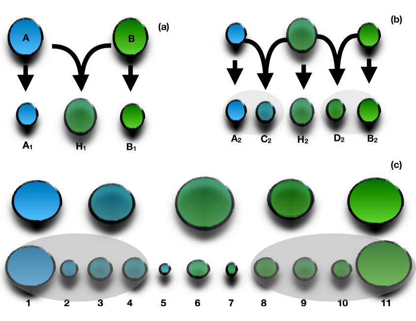
In generation 2 (and also thereafter) mating partners are selected from pools of size 400. Thus, if a first parent is selected from $A_{1}$ ($B_{1}$), the probability that the second parent is chosen from the hybrid group $H_{1}$ or from $B_{1}$ ($A_{1}$) is negligible. However, if a first parent is selected from $H_{1}$ the second parent can be taken from any of the three groups with significant probabilities. The second generation, therefore, has five groups, that we term $A_{2}$, $B_{2}$, $H_{2}$, $C_{2}$ and $D_{2}$, as illustrated in Figure 9b). However, the genetic similarity between individuals from groups $C_{2}$ and $A_{2}$ and between individuals from groups $D_{2}$ and $B_{2}$ is $0.975e^{-8\mu}$ meaning that, according to our criterion of $q_{0}=0.97$, groups $C_{2}$ and $A_{2}$ and groups $D_{2}$ and $B_{2}$ belong to the same species. This is illustrated in Figure 9c.

In generation 3 there are still 2 robust species (with about 870 individuals each) and 1 hybrid group, as in Figure 9c) (we have omitted the arrows indicating the origin of each group in order to make the illustration cleaner). Tracking the evolution of these subgroups along the following generations, one can observe that this pattern of more and more groups persists until a third species, with internal similarities larger than $q_{0}=0.97$, forms. The size of this hybrid species slowly decreases until its complete extinction in about 20 generations.

4 Comparison with Empirical Data

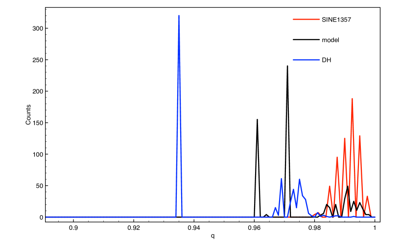
Although the model presented here discards any effects of spatial structure or selection, we have attempted to compare our results with empirical data. In what follows we compare the results of our simulations with a subgroup of African cichlids, the Haplochromines of Lake Victoria. Samonte et al. [51] have analyzed the genetic variability of four species of the haplochromine family collected from the Lake Victoria. The authors have compared the genetic similarity of the four cichlid species in five loci of nuclear DNA. Here we used data from the SINE1357 locus, which has been used to study the phylogeny of salmon species [52] and whales [53].

The authors have compared the genetic similarity of 36 individuals: 15, 16, 1 and 4 from Haplochromis fischeri, Ptyochromis xenognathus, Haplochromis chilotes and Haplochromis sp. “rock kribensis” species, respectively. The red line in Figure 10 corresponds to the histogram of similarity. It can be observed that there is a high degree of similarity among all species. In order to compare with results from the model considered here, we procedure as follow: First, we considered a population with 2000 individuals with a pool size equals to 500 individuals, which gives a $q_{0}$ equals to 0.974. Second: from the entire population, we select the four most similar (among them) species representing the four species from [51] and, third, we take, randomly, 15, 16, 1 and 4 individuals from these species. The histogram of these 36 individuals is shown by the black line in Figure 10. It is noticeable that the similarity between many individuals is very consistent with the similarity of the individuals from [51]. The main difference with experimental data is the two peaks around $q=0.96$ and $q=0.97$. We believe the main reason for such difference is that we have compared the infinite genome of the theoretical population while only a small fraction of the genome in the real population. We also compared the similarity between individuals from a theoretical population that evolved according to the Derrida-Higgs model [35] using $q_{min}=q_{0}=0.974$, shown by the blue line in Figure 10. One can see that only the threshold for genetic similarity is not enough to promote the good qualitative agreement as the assortative model and the experimental data.

Figure 10: Similarity between 36 individuals of four species: Red line is the similarity of the SINE1357 locus of real individuals, the black line is the result obtained with our model and the blue line corresponds to the Derrida-Higgs model .

5 Discussion

In this work we have considered a variation of the DH model in which the genetic threshold for reproduction compatibility is completely eliminated and replaced by a pure assortative mating mechanism. In our model each individual chooses for mating the most similar partner it can find in a random pool of size $N$, no matter how dissimilar it might be. Figure 2 shows that if the first parent can choose its mate from a pool of individuals of sufficiently large size, the histogram of similarities $q$’s does exhibit peaks below the asymptotic value $q_{conv}$. However, for small pools, a different dynamics take place, as illustrated in Figure 3 for $N=10$ (left panels). In these cases the distribution might break into clusters centered at $q>q_{conv}$ but the inter-cluster similarity is still large. These clusters are genetically close to each other and unstable. Since the pool is too small the likelihood that an individual of a cluster will select a pool consisting of individuals belonging solely to other clusters is high, making the clusters merge by the introduction of hybrids. As pool size increases the genetic distance between the clusters also increases and the peak representing inter-cluster similarity moves to the left of $q_{conv}$. For $N=30$, the clusters are still unstable and species prone to merging with one another, as illustrated in Figure 3 (right panels). For large pools the probability that the pool contains individuals of the same cluster is large, maintaining the species cohesion. However, merging is always possible since reproduction between any pair produces viable offspring. Thus, mating between individuals from different clusters does take place, generating hybrids and potentially merging species.

Our results demonstrate that assortative mating can lead to formation of clusters of individuals with high degree of similarity among themselves but with low degree of similarity with individuals belonging to other clusters. The number of species in the population, however, fluctuates in time, as shown in Figure 6. For small and medium pool sizes, there is a clear tendency of increasing the number of species as the pool size increases. However, for pool sizes larger than approximately 15-20% of the population, the behavior is more complex. In this regime the number of species is more sensitive to the reference value $q_{0}$. This fact can be understood as follows: if the pool size $N$ is a considerable fraction of the total population, the probability that the individual with the highest similarity with the first parent is in this pool is $N/M$, which is large by hypothesis. Moreover, even if the individual with highest similarity is not present in the pool, it is very likely that the highest similarity between the first parent and the individuals from the pool is very close to the highest similarity between the first parent and an individual from the population.

It is important to compare the model presented in this work with the one introduced in [35] where a minimum similarity is required in order to produce offspring (Figure 6). Within the error bars, both models provide almost the same number of species for small and medium pool size. On the other hand, when the pool size is a considerable fraction of the population, the purely assortative model leads to a larger number of species. This behavior is a consequence of the fact that, for large pool sizes, assortative mating can be more restrictive than the constraint of minimum similarity. On average, the similarity between parents in DH model is smaller than the similarity of the parents in the assortative model when the pool size is a considerable fraction of the population.

Finally, we have compared our model with data from a subgroup of cichlids from Victoria lake. Although our model is very simple and discards important features of the real dynamics (such as spatial structure, finite character of the real genomes and other selective forces), we obtained qualitative good agreement with the data, slightly better than that provided by the Derrida-Higgs model with a genetic threshold.

To summarize, we have introduced an evolutionary model based purely on assortative mating, without a genetic threshold that impairs reproduction. In the model individuals mate with the most similar individual in their pool of potential partners. We have shown that this condition alone can lead to the formation of clusters of genetically similar individuals. Although the absence of reproductive isolation makes the definition of species dependent on the identification of these clusters, which has a degree of subjectivity, these results show that species can potentially emerge from sympatric condition and without the need of an arbitrary genetic threshold to create reproductive isolation. We have studied the formation and evolution of a hybrid species formed by mixing two isolated species during a single generation of environmental disturbance. Restoring the environmental integrity in the next generation results in the formation of a hybrid species that slowly decreases in abundance and finally goes extinct, as observed in empirical studies.

Acknowledgments: M.A.M.A. acknowledges financial support from CNPq (grant 302049/2015-0) and FAPESP (grants 2016/06054-3 and 2015/11985-3). C.L.N. Costa. was supported by Capes, grant 302049/2015-0.

References

- [1] Mayr E 1942 Systematics and the origin of species, from the viewpoint of a zoologist (Harvard University Press)
- [2] Mallet J 1995 Trends in Ecology & Evolution 10 294–299
- [3] Paterson H E 1985
- [4] Templeton A R 1989 The units of evolution: Essays on the nature of species 159–183
- [5] Van Valen L 1976 Taxon 233–239
- [6] Wiley E O 1978 Systematic zoology 27 17–26
- [7] Cracraft J 1987 Biology and philosophy 2 329–346
- [8] Queiroz K and Donoghue M J 1988 Cladistics 4 317–338
- [9] Shaw K 2001 Journal of Evolutionary Biology 14 880–882
- [10] Baker R J and Bradley R D 2006 Journal of mammalogy 87 643–662
- [11] Harrison R G and Larson E L 2014 Journal of Heredity 105 795–809
- [12] Jiang Y, Bolnick D I and Kirkpatrick M 2013 The American Naturalist 181 E125–E138 pMID: 23669548
- [13] Jiang Y, Bolnick D I and Kirkpatrick M 2013 The American Naturalist 181 E125–E138
- [14] Arias C F, Rosales C, Salazar C, Castaño J, Bermingham E, Linares M and McMillan W O 2012 Molecular Ecology 21 5778–5794 ISSN 1365-294X
- [15] Kocher T D 2004 Nature Reviews Genetics 5 288
- [16] Dieckmann U 2004 Adaptive Speciation Cambridge Studies in Adaptive Dynamics (Cambridge University Press) ISBN 9780521828420
- [17] Seehausen O, Van Alphen J J and Witte F 1997 Science 277 1808–1811
- [18] Kirkpatrick M and Ravigné V 2002 the american naturalist 159 S22–S35
- [19] Coyne J and Orr H 2004 Speciation (Sinauer Associates, Sunderland, MA)
- [20] Gavrilets S 2004 Fitness Landscapes and the Origin of Species (Princeton University Press, Princeton, NJ)
- [21] Kondrashov A S and Shpak M 1998 Proceedings of the Royal Society of London. Series B: Biological Sciences 265 2273–2278
- [22] Fry J D 2003 Evolution 57 1735–1746
- [23] De Cara M, Barton N and Kirkpatrick M 2008 The American Naturalist 171 580–596
- [24] Kirkpatrick M 2000 Proceedings of the Royal Society of London B: Biological Sciences 267 1649–1655
- [25] Kirkpatrick M and Nuismer S L 2004 Proceedings of the Royal Society B: Biological Sciences 271 687
- [26] King D M, Scott A D and Bahar S 2017 Royal Society Open Science 4 170005
- [27] Rice W R 1984 Evolution 38 1251–1260 ISSN 00143820, 15585646
- [28] Rice W R and Hostert E E 1993 Evolution 47 1637–1653 ISSN 00143820, 15585646
- [29] Gavrilets S, Li H and Vose M D 2000 Evolution 54 1126 ISSN 0014-3820
- [30] Hoelzer G a, Drewes R, Meier J and Doursat R 2008 PLoS Computational Biology 4 e1000126 ISSN 1553-7358
- [31] Fitzpatrick B M, Fordyce J a and Gavrilets S 2009 Journal of evolutionary biology 22 2342–7 ISSN 1420-9101
- [32] de Aguiar M A M, Baranger M, Baptestini E M, Kaufman L and Bar-Yam Y 2009 Nature 460 384–387 ISSN 1476-4687
- [33] Dieckmann U and Doebeli M 1999 Nature 400 354–7
- [34] Kondrashov A S and Kondrashov F A 1999 Nature 400 351
- [35] Higgs P G and Derrida B 1991 Journal of Physics A: Mathematical and General 24 L985
- [36] de Aguiar M A M 2017 Journal of Physics A: Mathematical and Theoretical 50 085602
- [37] Martins A B, de Aguiar M A M and Bar-Yam Y 2013 Proceedings of the National Academy of Sciences 110 5080–5084
- [38] Baptestini E M, de Aguiar M A M and Bar-Yam Y 2013 Theoretical ecology 6 213–223
- [39] Schneider D M, Baptestini E M and de Aguiar M A M 2016 Journal of biological physics 42 235–245
- [40] Bateson W 1909 Heredity and variation in modern lights, pp. 85–101 in Darwin and Modern Science, edited by Seward AC (Cambridge University Press, Cambridge, UK)
- [41] Dobzhansky T 1937 Genetics and the Origin of Species (Columbia University Press, New York)
- [42] Muller H J 1939 Biological Reviews 14 261–280
- [43] Muller H 1942 Isolating mechanisms, evolution, and temperature Biol. Symp. vol 6 pp 71–125
- [44] Arnegard M E and Kondrashov A S 2004 Evolution 58 222–237
- [45] Turner G F and Burrows M T 1995 Proceedings of the Royal Society of London. Series B: Biological Sciences 260 287–292
- [46] Servedio M R and Bürger R 2014 Proceedings of the National Academy of Sciences 111 8113–8118 ISSN 0027-8424
- [47] Ng A Y, Jordan M I and Weiss Y 2002 On spectral clustering: Analysis and an algorithm Advances in neural information processing systems pp 849–856
- [48] Von Luxburg U 2007 Statistics and computing 17 395–416
- [49] Schumer M, Powell D L, Delclós P J, Squire M, Cui R, Andolfatto P and Rosenthal G G 2017 Proceedings of the National Academy of Sciences
- [50] Fisher H S, Wong B B and Rosenthal G G 2006 Proceedings of the Royal Society B: Biological Sciences 273 1187–1193
- [51] Samonte I E, Satta Y, Sato A, Tichy H, Takahata N and Klein J 2007 Molecular Biology and Evolution 24 2069–2080
- [52] Murata S, Takasaki N, Saitoh M and Okada N 1993 Proceedings of the National Academy of Sciences 90 6995–6999
- [53] Nikaido M, Rooney A P and Okada N 1999 Proceedings of the National Academy of Sciences 96 10261–10266