Fusion of Camera Model and Source Device Specific Forensic Methods for Improved Tamper Detection

Abstract

PRNU based camera recognition method is widely studied in the image forensic literature. In recent years, CNN based camera model recognition methods have been developed. These two methods also provide solutions to tamper localization problem. In this paper, we propose their combination via a Neural Network to achieve better small-scale tamper detection performance. According to the results, the fusion method performs better than underlying methods even under high JPEG compression. For forgeries as small as 100$\times$100 pixel size, the proposed method outperforms the state-of-the-art, which validates the usefulness of fusion for localization of small-size image forgeries. We believe the proposed approach is feasible for any tamper-detection pipeline using the PRNU based methodology.

Keywords PRNU  $\cdot$ CNN $\cdot$ Neural Network $\cdot$ source camera $\cdot$ identification $\cdot$ source camera verification $\cdot$ verification $\cdot$ digital forensics

1 Introduction

Digital images forgeries have become increasingly common in social media, causing a reduction of confidence in media found on the Internet. Because of this, many methods have been developed to detect tampered images, including the use of the Photo-Response Non-Uniformity (PRNU) noise based Source Camera Verification (SCV) [1]. PRNU based SCV works with a PRNU camera fingerprint which is first computed from multiple still images known to be taken by a specific camera. Then, the PRNU noise extracted from a query image is correlated with this fingerprint to determine if it was taken with the given camera. PRNU based SCV has been applied for tamper detection by matching the camera fingerprint on a block by block basis with the query image. Blocks within a tampered region of the query image will have a low correlation with the fingerprint as opposed to blocks that have not been tampered.

Since SCV is based on a correlation operation, using PRNU for tamper detection can be challenging when the tampered region is small, especially in textured regions. There have been many approaches that have been developed to address these challenges. One such technique assumes the existence of a linear relation between image content and PRNU similarity and applies it on each image block to predict correlation values [2]. Tampering is then detected based on a significant deviation of the actual correlation from the predicted value. Another approach focuses on changes to the denoising filter and the denoiser output [3, 4], citing the deficiencies of the denoiser that prevent tamper detection. Some other notable attempts included refining the detector output by applying segmentation [5], statistical methods to improve the localization map [6], and multi-scale strategies [7] to improve localization performance.

The media forensics community has recently started to incorporate deep learning techniques, especially CNN (Convolutional Neural Network) based methods to solve media forensics problems. For example, in [8], a multi-scale CNN model was used to detect and localize forged regions. In [9], a CNN based method for detecting forged regions from small image blocks was proposed. Also, in [10, 11], a method for source Camera Model Identification (CMI) using CNN was proposed and in [12] a universal manipulation detector using CNN was presented. However, this type of detectors require vast amounts of data for training, which may not be available in most cases and are vulnerable to adversarial attacks [13].

Unlike SCV which is often less than effective with small tampered regions [1, 7], CNN based techniques have been shown to perform well on tampered regions as small as $64\times 64$ pixels [9].Such CNN based techniques, as we show later, do not perform well under high compression, and PRNU based techniques do not perform well when tampered regions are with small size (e.g. $100\times 100$). However, it is intuitively clear that SCV and CMI are really exploiting different aspects of an image. SCV is based on device specific characteristics that is confined to the sensor array. CMI, on the other hand, attempts to capture all the processing in the camera pipeline after the image is captured. And while the former is robust to image processing operations, the latter is effective even when presented with smaller regions of an image. In this paper, we leverage the strengths of both these approaches with the proposed method. We extensively compare the performance of SCV, CMI, and the proposed method in the assessment of the integrity of small image blocks ($96\times 96$ pixels).

The proposed method, which we call the “Fusion” method, applies SCV and CMV on a block by block basis and fuses the results of the two using a neural network, to detect and localize image tampering. The performance of the proposed method is compared with the two methods in [6, 7] and is shown to yield better results with smaller forgery regions.

2 Background

The Fusion method incorporates traditional PRNU based SCV along with CNN based CMI, which was created from scratch albeit with inspirations from the literature. The following sub-sections briefly introduce these methods and outline their usage within the proposed method.

2.1 PRNU based Source Camera Verification

PRNU based SCV makes use of a noise pattern called Photo-Response Non-Uniformity (PRNU) noise. The PRNU noise pattern $F$ is caused by the variations in photo-sites response to intensity of light $I_{\mathrm{0}}$, which occurs due to inconsistencies inherent in sensor manufacturing process. The pattern is found to be unique for each camera sensor and it is detectable from digital images produced by digital cameras [14]. Other than PRNU, there is also random noise, denoted with $\Gamma$.

Following the simple imaging sensor output model in [14] with matrix notation: $I=I_{\mathrm{0}}+I_{\mathrm{0}}F+\Gamma$ that incorporates both types of noises, the pattern $F$ can be estimated with a set of noise estimates $N_{\mathrm{1}},...,N_{\mathrm{K}}$, and a $denoiser$, which is commonly referred as a Wavelet denoiser [15], s.t. $N=I-denoiser(I)$. Using these noise estimates, estimating the PRNU noise pattern of a camera’s sensor $\hat{F}$ can be computed using the MLE estimator in [14]. Verifying the source camera of a query image $I_{q}$ then only requires a Wavelet noise estimate $N_{q}$ of this image and the MLE-estimated PRNU pattern, $\hat{F}$ with normalized cross correlation $\rho=corr(N_{q},I_{q}\hat{F})$ or with peak-to-correlation-energy (PCE) formulation which applies some notable modifications [14] to normalized cross correlation.

2.2 CNN based Camera Model Identification

CNN consists of cascaded layers, which makes it useful to extract specific features from input images. In the convolution layer, the input data has the resolution of W${}_{I}\times$ H${}_{I}\times$ D_I (from now on, W denotes width, H height, and D depth) is convolved with a kernel with resolution W${}_{K}\times$ H${}_{K}\times$ D_K, which is initialized with random weights at the beginning and a specified value of stride. This operation produces a convolution map as the output. After the convolution layer, activation function such as Rectified Linear Unit (ReLU) is applied to avoid linearity.

In this work, the input data resolution W${}_{I}\times$ H${}_{I}\times$ D_I is selected as 96$\times$96$\times$3, the kernel size W${}_{K}\times$ H_K is selected as 3$\times$3 and max(0,x) function is used as the ReLU activation function as shown in Fig. 2. The pooling layer carries out down-sampling operation to produce smaller feature maps. The fully connected (FC) layer carries out a dot product between the input feature vector and randomly initialized filter vector. Class scores are also produced in the FC layer. Softmax layer carries out class scores coming from FC to probability scores so that the sum of all scores becomes 1.

In the CNN literature, many algorithms are used for updating kernel weights. We use the most common one, the stochastic gradient descent algorithm. To train the CNN for camera model identification (CMI), we feed it with images from different camera models and labels referencing to the class of the images. As we want this CNN network to generate probability scores for two classes, i.e. “target camera model” ($\mathrm{H}_{1}$) and “other camera model” ($\mathrm{H}_{0}$), for each camera model. If an image from a different camera model is given to the CNN, then it would compute a higher probability for other class, $\mathrm{H}_{0}$.

3 Proposed Method

CNN based CMI (Method 1) basically distinguishes camera models according to the interpolation feature of the camera. Using small size blocks ($\leq$250) as input allows it to detect small-size copy-paste forgeries. PRNU-based SCV (Method 2), on the other hand, recognizes the source camera, based on the stationary features of the camera sensor. Detection of tampered regions is also possible with Method 2. However, as resolution of the selected input window decreases, performance also decreases. We propose to combine (fuse) these two methods that can work better than each method individually. We expect that since Method 1 and Method 2 contain statistically different information, it will give a more reliable result when combined.

Figure 1: Block Diagram for Fusion Method Approach

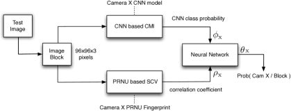
Method 1 produces probability value as an output. Method 2 produces correlation between fingerprint and noise of image block. A simple NN network has been created to weight these two outputs at the best rate. Briefly, output information from Method 1 and Method 2 are given as input to NN.(Fig. 1)

In order to use the Fusion method, we assume that we have the model information and the PRNU fingerprint of the device. This way, we can apply both methods and produce a single outcome through the NN.

Following steps are repeated for each input image block.

1. Obtain the probability value output from CNN based CMI (Method 1),

2. Compute the correlation value from the PRNU based SCV (Method 2),

3. Combine the correlation value (from Method 1) with the probability value (from Method 2) using the proposed NN.

For the first step, the CNN network is trained using $96\times 96$ pixel image blocks. After training, the network is able to produce probability value $\phi$ for the target camera class $H_{1}$

In the second step, correlation value $\rho$, between PRNU noise in same image blocks from the first step, and their corresponding PRNU fingerprint blocks are calculated.

In the third step, we combine the above two outcomes ($\rho$ and $\phi$). To do so, a neural network (NN) was trained which gets the values of $\rho$ and $\phi$ as input and produces a probability score for the existence of a forgery. This way, we can generate a decision map by sliding over the image $96\times 96$ pixels block at a time with a small amount of shift.

Label	Make	Model	Resolution
C1	Samsung	S3 Mini	2560$\times$1920
C2	Apple	iPhone 4s	3264$\times$2448
C3	Huawei	P9	3969$\times$2976
C4	LG	D290	3264$\times$2448
C5	Apple	iPhone 5c	3264$\times$2448
C6	Samsung	Tab3	2048$\times$1536
C7	Apple	iPhone 4	2592$\times$1936
C8	Samsung	Galaxy S3	3264$\times$2448
C9	Sony-Xperia	Z1 Compact	5248$\times$3936
C10	Apple	iPad2	960$\times$720
C11	Huawei	P9 Lite	4160$\times$3120
C12	Microsoft	Lumia 640 LTE	3264$\times$1840
C13	Apple	iPhone 6 Plus	3264$\times$2448
C14	Apple	iPad Mini	2592$\times$1936
C15	Wiko	Ridge 4G	3264$\times$2448
C16	Samsung	Trend Plus	2560$\times$1920
C17	One Plus	A3000	4640$\times$3480

Table 1: The cameras used in the experiments.

4 Dataset and Experimental Setup

The Vision dataset in [16], was preferred in this study since it has images from 29 different contemporary camera models. For each camera model, we used images labeled as "flat" and "nat" (as natural). Though there are 29 models in total, 17 camera models of 21 devices were used in this study (Table 1). Only one device was used from each camera model for training operations as a target camera. The additional four devices were used to evaluate small forgery localization performance against different devices of the same model, which is explained in Section 5.3. A total of 160 nat images were used per device in all experiments (Table 2). 100 of these nat images were used only in CNN training/testing, and up to 50 images from the remaining nat images were separated for NN training and method comparison. The rest (10 images) were used for determining the optimum F-score threshold value for comparison with the other methods in Section 6. Let us denote these 10 images as the set $\mathcal{F}$. All the image sets were mutually exclusive, in other words, no data was used more than once in any image set throughout this experiment.

CNN Training/ Testing		NN Training/ Method Comp.		Threshold Decision
Label	#	Label	#	Label	#
$\mathcal{C}_{\mathrm{tr}}$	80	$\mathcal{S}_{\mathrm{tr}}$	40	-	-
$\mathcal{C}_{\mathrm{ts}}$	20	$\mathcal{S}_{\mathrm{ts}}$	10	-	-
$\mathcal{C}$	100	$\mathcal{S}$	50	$\mathcal{F}$	10

Table 2: Image sets used in experiments for target camera. Here, # denotes number of images in image sets.

4.1 CMI Setup (Method 1)

For CNN training, blocks of size $96\times 96$ pixels were extracted randomly from each image from two classes, s.t. 500 blocks from images within the target (correct) class, and 50 blocks from images within the other class.

Figure 2: CNN model used in camera model classifier

The number of blocks we used for the CNN are given in Table 3, where $\mathcal{C}_{\mathrm{tr}}$ and $\mathcal{C}_{\mathrm{ts}}$ denote the sets of images used for training and testing respectively, whereas the numbers show the number of image blocks in each set used.

	# of Images		# of Blocks
Set Name	Target Camera	Other Camera	Target Camera	Other Camera
$\mathcal{C}_{\mathrm{tr}}$	80	1280	40k	64k
$\mathcal{C}_{\mathrm{ts}}$	20	320	10k	16k
$\mathcal{C}$	100	1700	50k	80k

Table 3: The data used in the CMI setup. Blocks refer to $96\times 96$ pixels worth image patches used in CNN training and test phases

In the related literature, simple models are shown to produce successful results [17]. Our preliminary experiments showed CNN models with small kernel sizes perform better than larger kernels for CMI. For this reason we inspired by VGG [18], which employs a small size kernel filter. We experimented with different hyper-parameters and layer structures and settled with the architecture that gave the best performance, as shown in Fig. 2. The CNN network was trained for each of the 20 camera models. The training phase was stopped after 50 epochs.

4.2 SCV Setup (Method 2)

For each camera model, the PRNU fingerprint was estimated using all of the available flat images. Each camera had at least 70 flat images. We used the PRNU method as described in [14]. Please note that PRNU noise of the image blocks used here were cropped from the PRNU noise extracted from the full image.

Image blocks in the set $\mathcal{S}_{\mathrm{ts}}$ were used for performing PRNU based source camera identification. To ensure fairness, the image blocks in the $\mathcal{S}_{\mathrm{ts}}$ set were used for comparison. However, as the performance of image noise extraction algorithms get worse for small image regions, we avoid extracting the noise from the image blocks in $\mathcal{S}_{\mathrm{ts}}$, and estimated PRNU noise $N$ from whole images.

These noise estimates were then cropped from the identical coordinates of each $96\times 96$ pixel image blocks in set $\mathcal{S}_{\mathrm{ts}}$. Then, they were correlated with the PRNU fingerprint blocks extracted from the identical coordinates of the corresponding camera PRNU fingerprints.

Some of the images placed in the set $\mathcal{S}_{\mathrm{ts}}$ were found to produce unexpectedly lower-than-threshold PRNU similarity (50 in terms of PCE) values against their matching PRNU fingerprints. We attributed such outcomes to possible mistakes in the dataset labels. For this reason, the image blocks from these images were excluded from the set $\mathcal{S}$.

Figure 3: Illustration of image sets used during the training and testing phases.

4.3 Combining CMI and SCV outcomes

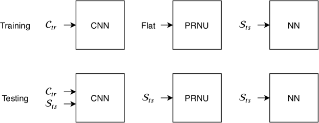
The Fusion method comprises 3 steps in total. First, the probability value was acquired from the CNN classifier, then the correlation value from the PRNU method was computed and lastly, the NN part is trained to combine these two and produces the final probability value. Therefore, the third step forms the actual output of the Fusion method.

We construct a simple artificial NN using $\rho$ (from PRNU) and $\phi$ (from CNN classifier) values obtained from the $\mathcal{S}_{\mathrm{tr}}$, which includes the image blocks corresponding to $\mathrm{H_{1}}$ and the $\mathrm{H_{0}}$ cases. Therefore the NN can learn from both the matching ($\mathrm{H_{1}}$) and the non-matching ($\mathrm{H_{0}}$) cases.

For the NN, the number of blocks we used is denoted by $\mathcal{S}_{\mathrm{ts}}$ and $\mathcal{S}_{\mathrm{tr}}$ for the number of training blocks and testing blocks as shown in Table 4.

Let us denote each RGB image block in $\mathcal{S}_{\mathrm{tr}}$ and $\mathcal{S}_{\mathrm{ts}}$, by its source, i.e. the source coordinates ($\mathrm{i}$, $\mathrm{j}$) and the index of the source image ($\mathrm{k}$) with the symbol $B_{\mathrm{ijk}}$, the corresponding PRNU noise with $N_{\mathrm{ijk}}$. Similarly, the PRNU fingerprint estimate of camera $\mathrm{x}$ for the same coordinates is denoted by $F_{\mathrm{ij}}^{\mathrm{x}}$. These are then used to generate $\rho_{\mathrm{ijk}}$, as expressed in the Eq. (2). The CNN tests, on the other hand, generates the $\phi_{\mathrm{ijk}}$ values in (1). Also, in the Eq. (1), $\mathrm{CNNmodel^{x}}$ term refers to model learned from the CNN training of camera $\mathrm{x}$ and $f_{\mathrm{{CNN}}}$ refers to the CNN based CMI function.

$$\phi_{\mathrm{ijk}}=f_{\mathrm{{CNN}}}(B_{\mathrm{ijk}},\mathrm{CNNmodel^{x}})$$ (1)

$$\rho_{\mathrm{ijk}}=corr(N_{\mathrm{ijk}},B_{\mathrm{ijk}}F_{\mathrm{ij}}^{x})$$ (2)

In our experiments, we find that the model performs best with 2 hidden layers and 10 nodes for each hidden layer. $\rho$ and $\phi$ values, obtained from $\mathcal{S}_{\mathrm{tr}}$, were used for the NN training and the learned model will be denoted by $\mathrm{NNmodel}^{\mathrm{x}}$. Thus, when $B_{\mathrm{ijk}}$ is given as an input to $f_{\mathrm{NN}}$, the neural network function, the probability of tampering for a given $B_{\mathrm{ijk}}$, denoted by $\theta_{\mathrm{ijk}}$ is produced Eq. (3).

$$\theta_{\mathrm{ijk}}=f_{\mathrm{NN}}(\rho_{\mathrm{ijk}},\phi_{\mathrm{ijk}},\mathrm{NNmodel}^{\mathrm{x}})$$ (3)

5 Results and Discussion

In this section, we provide results of the proposed method in different settings. and compare results with benchmarks using two different methods in the literature.

5.1 Receiver Operating Characteristics of the Proposed Method

	CNN	# of	AUC Values on set $\mathcal{S}_{\mathrm{ts}}$
Label	Acc.	Blocks
	on $\mathcal{C}_{\mathrm{ts}}$	$\mid\mathcal{S}_{\mathrm{ts}}\mid$/$\mid\mathcal{S}_{\mathrm{tr}}\mid$	PRNU	CNN	Fusion
C1	92%	13.9k / 55.6k	0.97	0.96	0.99
C2	80%	14.5k / 58k	0.95	0.92	0.99
C3	95%	10.8k / 43.2k	0.91	0.99	0.99
C4	94%	14.2k / 56.8k	0.95	0.98	0.99
C5	93%	13.7k / 54.8k	0.99	0.96	0.99
C6	97%	13k / 52k	0.98	0.96	0.99
C7	97%	14.5k / 58k	0.98	0.99	0.99
C8	94%	14.5k / 58k	0.98	0.98	0.99
C9	99%	14.5k / 58k	0.99	0.99	0.99
C10	85%	14.5k / 58k	0.94	0.96	0.98
C11	96%	10.6k / 42.4k	0.97	0.99	0.99
C12	95%	14.5k / 58k	0.96	0.99	0.99
C13	89%	14.5k / 58k	0.98	0.94	0.99
C14	85%	13.5k / 54k	0.99	0.91	0.99
C15	92%	14.5k / 58k	0.98	0.99	0.99
C16	85%	14.5k / 58k	0.95	0.97	0.99
C17	95%	12k / 48k	0.99	0.98	0.99

Table 4: The performance of underlying methods. Accuracy values are denoted with (“Acc”). The AUC values from the CNN network have been obtained from set ${C}_{\mathrm{ts}}$ and the AUC values were calculated from their ROC’s. ${S}_{\mathrm{ts}}$ represents the amount of blocks in the test image set, whereas ${S}_{\mathrm{tr}}$ represents the amount of blocks in the training image set.

In this section, we evaluate the performance of the proposed Fusion method against its underlying methods to quantify the improvement for tamper detection. To test the NN performance, the correlation value $\rho_{\mathrm{ijk}}$, and the class probability $\phi_{\mathrm{ijk}}$ values are obtained from image blocks $B_{\mathrm{ijk}}$ s.t. $B_{\mathrm{ijk}}\in\mathcal{S}_{\mathrm{ts}}$. Then the performance metrics, Area Under the Curve (AUC) and ROC for each camera model were calculated using the outputs in Eqs. (1, 2 and 3). These metrics were calculated by counting the number of matching blocks and non-matching blocks for various threshold values, in the range of [-1,1] for the SCV output and [0,1] for the CMI and Fusion output.

Using the same blocks, the same performance metrics were also calculated with the PRNU and the CNN methods. The AUC values are given in Table 4.

5.2 Robustness under JPEG Compression

In our previous experiments, the Fusion method achieved high performance against small blocks from original images. However, it’s not clear how well the proposed method would perform with compressed test samples. In this subsection, we provide results to evaluate the robustness of the Fusion method against compression.

Figure 4: The average AUC values for various JPEG quality factors

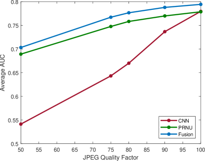
To do so, we reuse the previous experiment setup, with only one small modification: the image blocks in $\mathcal{S}_{\mathrm{ts}}$ were extracted from images compressed with 5 different JPEG quality factors.

It is known in the literature that the PRNU method is robust against JPEG compression. However, the same cannot be said for the CNN based CMI method as shown in Fig. 4. On images re-compressed with JPEG at various quality levels, Fusion worked reasonably well, in line with PRNU method. According to the results in Fig. 4, the Fusion method performed better than both the CNN based CMI and the PRNU based SCV at all compression rates, and reached an average of 23% improvement against CNN based CMI on images with the highest compression rate.

5.3 Usability of pre-trained camera models

Employing the proposed method in current tamper-detection schemes only incurs initial computation costs for unknown camera models. Thus, in other words, only new camera models (not existed in a database) need to be trained through the CNN and NN outlined in this paper.

Recall that in the previous sections, experiments with Fusion were conducted on images strictly coming from one device for each model. In this section, we evaluate the performance of the Fusion with images from new devices with the same models where we already have NN and CNN models. Although CNN models are only camera-model-specific, the NN model is trained with device-specific correlation map, which may cause it to become device-specific as well. These additional devices and their models are given in Table 5. The test results show how the Fusion method would perform when the training device and the test device are different, but sharing the same model. The results show that the CNN based CMI and the NN models work successfully for images from another device of the same camera model. As long as we have a PRNU fingerprint of a device of a known camera model, the proposed method can be used for tamper detection regardless of the source camera device.

Note, that the number of test images and the number of blocks were the same as in Section 5.1. For each device in the Table 5, $\mathcal{S}_{\mathrm{ts}}$ was created and the tests were performed on this set.

Device	Camera	AUC Values on set $\mathcal{S}_{\mathrm{ts}}$
Label	Model	PRNU	CNN	Fusion
C2,Dev-2	iPhone 4s	0.965	0.855	0.982
C5,Dev-2	iPhone 5c	0.959	0.837	0.976
C5,Dev-3	iPhone 5c	0.916	0.902	0.976
C1,Dev-2	S3 Mini	0.962	0.939	0.984

Table 5: The details of the selected same camera models with different devices and their respective AUC values using the pre-trained models. The AUC values were calculated from ROC’s. (Dev: Device)

6 Tamper Detection Benchmarks

In this section, we evaluate the performance of the proposed method against other PRNU based tamper detection methods in the literature.

6.1 Methods

For benchmarking tamper detection rates, we selected two publicly released PRNU based tamper detection methods. The first one was the multi-scale fusion (which will be denoted as “MSF” from now on) strategy in [7, 19]. Briefly, this method produces heat-maps using the standard PRNU method through different window sizes. These heat-maps are then fused using Conditional Random Fields (CRF) thus producing binary-maps. Since each heat-map is made from windows of different sizes, smaller windows-sizes are more suitable for detecting smaller tampered regions, and similarly, larger window-sizes are better for larger tampered regions. Therefore, compared to the standard PRNU method, this method can produce better true positive and false positive rates.

The other method used for comparison was the Bayesian-MRF method in [6]. This method, (denoted as “MRF” ) replaces the constant false alarm rate with the Bayesian rule, uses BM3D non-local filtering instead of a Wavelet-based filter, and uses Markovian priors to model spatial dependencies of the image to provide better detection rate over the standard PRNU method.

Training for both methods was done using full images from the set $\mathcal{C}_{\mathrm{tr}}$ while CNN training of Fusion was done using blocks from the image set shown in Table 3. As all the three methods make use of PRNU fingerprint estimates, the same set of flat images were used to compute these estimates for each device.

6.2 Determining the Decision Threshold

We look for a decision threshold value to create a binary map of the output of the Fusion method for each camera model. We carry out this by measuring the F-score values, over a set of tampered images. The tampered images were generated using the image set $\mathcal{F}$, which consists of 10 images which were not used in any experiments.

(a) C5: iPhone 5c

(b) C11: P9 Lite

Figure 5: The average F-score measurements used for determining the threshold for two example camera models. In the Figures, the threshold values which gives the maximum average F-score is selected as the decision threshold with the Fusion method and highlighted with the red marker. The horizontal axis represents the threshold values, whereas the vertical axis represents the F-score values.

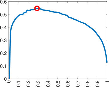
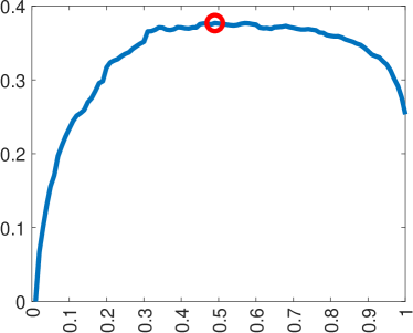
We applied 100 threshold values in the range of [0-1], and applied morphological opening operation through disc kernel with fixed-size (20px) radius on the binary map. Using the ground-truth for each tampered image, we then measured the F-score values. The F-score was computed with the following:

$$\textrm{F-score}=\frac{2\times\textrm{TP}}{2\times\textrm{TP}+\textrm{FP}+\textrm{FN}}$$ (4)

where in Eq. 4, TP stands for true positive, FP for false positive and FN for false negative. This way, we end up having 30 different F-score measurements (3 tampered region sizes for each image is set $\mathcal{F}$) for all threshold values. The F-score measurements are then averaged and the threshold value producing the best F-score value in Eq. 4 was selected as the threshold for each camera model. The averaged F-score measurements and the determined decision threshold values for two example cameras can be seen in Fig. 5.

	Tampered Region Size (pixels)
	400$\times$400			200$\times$200			100$\times$100
Label	Fusion	MRF	MSF	Fusion	MRF	MSF	Fusion	MRF	MSF
C1	0.60	0.52	0.71	0.33	0.27	0.46	0.12	0.03	0.07
C2	0.53	0.41	0.51	0.41	0.30	0.33	0.18	0.09	0.07
C3	0.64	0.16	0.39	0.38	0.00	0.02	0.09	0.00	0.00
C4	0.86	0.42	0.64	0.72	0.23	0.44	0.56	0.05	0.22
C5	0.69	0.75	0.84	0.58	0.58	0.69	0.20	0.07	0.13
C6	0.87	0.73	0.56	0.73	0.47	0.50	0.30	0.16	0.19
C7	0.92	0.69	0.82	0.83	0.51	0.69	0.31	0.16	0.36
C8	0.64	0.78	0.81	0.52	0.59	0.66	0.13	0.29	0.26
C9	0.86	0.53	0.88	0.75	0.35	0.73	0.58	0.03	0.23
C10	0.79	0.76	0.82	0.52	0.52	0.67	0.07	0.32	0.44
C11	0.57	0.48	0.55	0.30	0.30	0.29	0.07	0.00	0.01
C12	0.81	0.49	0.79	0.62	0.26	0.53	0.36	0.05	0.14
C13	0.67	0.49	0.57	0.45	0.29	0.43	0.19	0.15	0.15
C14	0.71	0.51	0.81	0.38	0.21	0.37	0.03	0.03	0.02
C15	0.83	0.76	0.77	0.70	0.62	0.65	0.48	0.38	0.30
C16	0.59	0.54	0.70	0.41	0.34	0.55	0.21	0.11	0.15
C17	0.75	0.33	0.53	0.53	0.10	0.31	0.13	0.02	0.16
Avg	0.73	0.57	0.70	0.56	0.38	0.53	0.26	0.13	0.19

Table 6: The F-scores from the benchmarks, w.r.t. to tampered region sizes. Camera details were given in Table 4. MSF represents the Multi-Scale Fusion method [7, 19], MRF represents the Bayesian-Markovian Random Fields method in [6]. Avg. have been calculated with F-score values from all tested images.

Figure 6: Examples with tampered region size of 400$\times$400 pixels. In each row, there are three tampered images from one camera model, ordered from C1 to C16 from top left to bottom right. The colors on the maps are coded as the following: green - true positives; blue - false negatives; red - false positives; black - true negatives. Only one threshold value was picked per each camera model as explained in Section 6 for Fusion method. Except for images from C10, images are cropped for better visualization.

Figure 7: Examples with tampered region size of 200$\times$200 pixels. In each row, there are three tampered images from one camera model, ordered from C1 to C16 from top left to bottom right. The colors on the maps are coded as the following: green - true positives; blue - false negatives; red - false positives; black - true negatives. Only one threshold value was picked per each camera model as explained in Section 6 for Fusion method. Except for images from C10, images are cropped for better visualization.

Figure 8: Examples with tampered region size of 100$\times$100 pixels. In each row, there are three tampered images from one camera model, ordered from C1 to C16 from top left to bottom right. The colors on the maps are coded as the following: green - true positives; blue - false negatives; red - false positives; black - true negatives. Only one threshold value was picked per each camera model as explained in Section 6 for Fusion method. Except for images from C10, images are cropped for better visualization.

6.3 Comparison

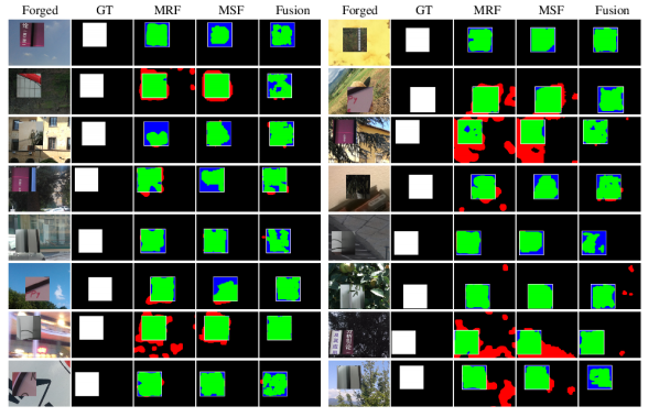
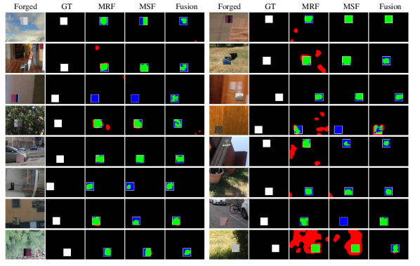
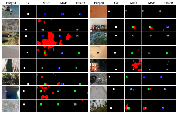
The methods were tested with the images from $S_{\mathrm{ts}}$ which, to recall, included 154 images across all camera devices. Note that this image set was used only for testing purposes, and no image in this set was included in any training phase of any method we compared. To evaluate tamper detection performance, we created copy-paste forgeries with the following sizes: 400$\times$400, 200$\times$200 and 100$\times$100 pixels and saved each of these images with the lossless format (PNG) leading to 462 tampered images. On average, 25 images per device were tested. Please note that for the Fusion, the same morphological treatment in Section 6 was applied on threshold-applied probability maps before computing the F-score values.

In order to make the comparison fair, a window-size of 96$\times$96 pixels was chosen for the MRF method to be in line with the Fusion approach (which uses 96$\times$96). However, as the MSF method inherently utilized multiple window-sizes, for MSF, we used the following 7 different sizes: 32$\times$32, 48$\times$48, 64$\times$64, 96$\times$96, 128$\times$128, 192$\times$192, 256$\times$256 pixels as stated in [7]. This may seem to be advantageous for the MSF method, as it has the advantage of utilizing more heat-maps, however, we believe adhering to the literature will lead to a more objective comparison. In Fig. 8, 7 and 6, one tampered image for each camera model are shown for various tampered region sizes.

In Table 6, the average F-score values for each method are provided. As seen in the Table, The proposed Fusion method performed better for all tampered region sizes. Overall, on 51 test cases (from 17 cameras and 3 different tampered region sizes) we tested, the Fusion method was the best performing in 34 cases, whereas for MSF there were 15 such cases and for MRF there were 2 such cases.

On experiments with the largest tampered region size setting, MSF worked best in terms of leading-cases (denoted with bold characters in Table 6), however, it is behind the Fusion method with 7% in terms of F-scores. We believe the multi-scale strategy employed by the MSF increased its advantage within this setting. Furthermore, there are few exceptions where the Fusion method performed consistently worse for a few cameras: C8 (Samsung Galaxy S3) and C10 (Apple iPad).

7 Conclusion

In this paper, we present a new technique for forgery detection, by using both of the model-specific and the device-specific features of a camera to achieve better small-scale tamper detection performance. To reach this goal, a CNN classifier for CMI and the traditional PRNU based SCV method were combined via a Neural Network. We call this the Fusion method.

We first study how much the proposed Fusion approach improves detection of forgeries over traditional methods and compared it against both CNN based CMI and PRNU based SCV methods. We found that Fusion performed better than both CNN based CMI (up to 10%), and PRNU based SCV (up to 10%) in detecting tampering using blocks originating from a different camera.

We also show that the CNN and NN models trained for the Fusion with specific camera models can be re-used for localization of forgeries on a tampered image captured with a new device from the same camera model. Furthermore, the robustness of the Fusion approach and its underlying detectors was compared. We found that the robustness of Fusion was better than the underlying methods.We believe that, training a CNN model with the knowledge of compression can increase the performance Fusion even further in such settings.

To complete the study, the proposed Fusion approach was compared against other PRNU-based enhanced forgery detection methods in the literature. Results with the proposed method were better in locating forgeries, where, on average, Fusion had 0.50, MSF had 0.44, and MRF had 0.35 in terms of F-scores for all tampered region sizes. Similarly, Fusion performed best on the smallest tampered region size we tested (100$\times$100 pixels), where it performed 92% better than MRF, and 39% than MSF. However, the performance of the proposed method w.r.t. other methods was found slightly poorer on larger tampered regions. The analysis window size of the proposed method can be adjusted to accommodate for larger tampered regions for such cases.

For future work, we will evaluate employing multi-scale strategies and compression aware deep networks to further improve the detection rates for forgeries of various size.

8 Acknowledgments

This material is based on research sponsored by DARPA and Air Force Research Laboratory (AFRL) under agreement number FA8750-16-2-0173. The U.S. Government is authorized to reproduce and distribute reprints for Governmental purposes notwithstanding any copyright notation thereon. The views and conclusions contained herein are those of the authors and should not be interpreted as necessarily representing the official policies or endorsements, either expressed or implied, of DARPA and Air Force Research Laboratory (AFRL) or the U.S. Government.

References

- [1] M. Chen, J. Fridrich, M. Goljan, J. Lukas, Determining Image Origin and Integrity Using Sensor Noise, IEEE Transactions on Information Forensics and Security 3 (1) (2008) 74–90. doi:10.1109/TIFS.2007.916285.
- [2] M. Chen, J. Fridrich, J. Lukáš, M. Goljan, Imaging sensor noise as digital x-ray for revealing forgeries, in: T. Furon, F. Cayre, G. Doërr, P. Bas (Eds.), Information Hiding, Springer Berlin Heidelberg, Berlin, Heidelberg, 2007, pp. 342–358.
- [3] G. Chierchia, D. Cozzolino, G. Poggi, C. Sansone, L. Verdoliva, Guided filtering for PRNU-based localization of small-size image forgeries, in: ICASSP, IEEE International Conference on Acoustics, Speech and Signal Processing - Proceedings, 2014, pp. 6231–6235. doi:10.1109/ICASSP.2014.6854802.
- [4] X. Lin, C. T. Li, Preprocessing Reference Sensor Pattern Noise via Spectrum Equalization, IEEE Transactions on Information Forensics and Security 11 (1) (2016) 126–140. doi:10.1109/TIFS.2015.2478748.
- [5] G. Chierchia, S. Parrilli, G. Poggi, L. Verdoliva, C. Sansone, PRNU-based detection of small-size image forgeries, in: 17th DSP 2011 International Conference on Digital Signal Processing, Proceedings, IEEE, 2011, pp. 1–6. doi:10.1109/ICDSP.2011.6004957.
- [6] G. Chierchia, G. Poggi, C. Sansone, L. Verdoliva, A bayesian-MRF approach for PRNU-based image forgery detection, IEEE Transactions on Information Forensics and Security 9 (4) (2014) 554–567.
- [7] P. Korus, J. Huang, Multi-scale fusion for improved localization of malicious tampering in digital images, IEEE Transactions on Image Processing 25 (3) (2016) 1312–1326. doi:10.1109/TIP.2016.2518870.
- [8] Y. Liu, Q. Guan, X. Zhao, Y. Cao, Image forgery localization based on multi-scale convolutional neural networks, in: Proceedings of the 6th ACM Workshop on Information Hiding and Multimedia Security, IH&MMSec ’18, ACM, New York, NY, USA, 2018, pp. 85–90. doi:10.1145/3206004.3206010.
- [9] L. Bondi, S. Lameri, D. Guera, P. Bestagini, E. J. Delp, S. Tubaro, Tampering Detection and Localization Through Clustering of Camera-Based CNN Features, in: 2017 IEEE Conference on Computer Vision and Pattern Recognition Workshops (CVPRW), IEEE, 2017, pp. 1855–1864. doi:10.1109/CVPRW.2017.232.
- [10] L. Bondi, L. Baroffio, D. Guera, P. Bestagini, E. J. Delp, S. Tubaro, First Steps Toward Camera Model Identification with Convolutional Neural Networks, IEEE Signal Processing Letters 24 (3) (2017) 259–263. arXiv:1603.01068, doi:10.1109/LSP.2016.2641006.
- [11] A. Tuama, F. Comby, M. Chaumont, Camera model identification with the use of deep convolutional neural networks, in: 2016 IEEE International Workshop on Information Forensics and Security (WIFS), IEEE, 2016, pp. 1–6. doi:10.1109/WIFS.2016.7823908.
- [12] B. Bayar, M. C. Stamm, A Deep Learning Approach to Universal Image Manipulation Detection Using a New Convolutional Layer, in: Proceedings of the 4th ACM Workshop on Information Hiding and Multimedia Security - IH&MMSec ’16, ACM Press, New York, New York, USA, 2016, pp. 5–10. doi:10.1145/2909827.2930786.
-
[13]
F. Marra, D. Gragnaniello, L. Verdoliva,
On
the vulnerability of deep learning to adversarial attacks for camera model
identification, Signal Processing: Image Communication 65 (2018) 240 – 248.
doi:https://doi.org/10.1016/j.image.2018.04.007.
URL http://www.sciencedirect.com/science/article/pii/S0923596518303217 - [14] M. Goljan, J. Fridrich, T. Filler, Large scale test of sensor fingerprint camera identification, in: SPIE Electronic Imaging, International Society for Optics and Photonics, 2009, pp. 72540I—-72540I.
- [15] J. Lukáš, J. Fridrich, M. Goljan, Digital Camera Identification From Sensor Pattern Noise, IEEE Transactions on Information Forensics and Security 1 (2) (2006) 205–214. doi:10.1109/TIFS.2006.873602.
- [16] D. Shullani, M. Fontani, M. Iuliani, O. A. Shaya, A. Piva, Vision: a video and image dataset for source identification, EURASIP Journal on Information Security 2017 (1) (2017) 15. doi:10.1186/s13635-017-0067-2.
- [17] L. Bondi, D. Güera, L. Baroffio, P. Bestagini, E. Delp, S. Tubaro, A Preliminary Study on Convolutional Neural Networks for Camera Model Identification, in: Electronic Imaging, Vol. 2017, 2017, pp. 67–76.
- [18] K. Simonyan, A. Zisserman, Very Deep Convolutional Networks for Large-Scale Image Recognition, Information and Software Technology 51 (4) (2014) 769–784. arXiv:1409.1556, doi:10.1016/j.infsof.2008.09.005.
- [19] P. Korus, J. Huang, Multi-scale analysis strategies in prnu-based tampering localization, IEEE Transactions on Information Forensics and Security 12 (4) (2017) 809–824. doi:10.1109/TIFS.2016.2636089.