Robust Optimization for Fairness
with Noisy Protected Groups

Serena Wang
UC Berkeley
Google Research
serenalwang@berkeley.edu
&Wenshuo Guo footnotemark:
UC Berkeley
wsguo@berkeley.edu
Harikrishna Narasimhan
Google Research
hnarasimhan@google.com
&Andrew Cotter
Google Research
acotter@google.com
Maya Gupta
Google Research
mayagupta@google.com
&Michael I. Jordan
UC Berkeley
jordan@berkeley.edu
First two authors have equal contributions.
Abstract

Many existing fairness criteria for machine learning involve equalizing some metric across protected groups such as race or gender. However, practitioners trying to audit or enforce such group-based criteria can easily face the problem of noisy or biased protected group information. First, we study the consequences of naïvely relying on noisy protected group labels: we provide an upper bound on the fairness violations on the true groups G𝐺G when the fairness criteria are satisfied on noisy groups G^^𝐺\hat{G}. Second, we introduce two new approaches using robust optimization that, unlike the naïve approach of only relying on G^^𝐺\hat{G}, are guaranteed to satisfy fairness criteria on the true protected groups G𝐺G while minimizing a training objective. We provide theoretical guarantees that one such approach converges to an optimal feasible solution. Using two case studies, we show empirically that the robust approaches achieve better true group fairness guarantees than the naïve approach.

1 Introduction

As machine learning becomes increasingly pervasive in real-world decision making, the question of ensuring fairness of ML models becomes increasingly important. The definition of what it means to be “fair” is highly context dependent. Much work has been done on developing mathematical fairness criteria according to various societal and ethical notions of fairness, as well as methods for building machine-learning models that satisfy those fairness criteria [see, e.g., 21, 32, 53, 41, 58, 14, 25, 55].

Many of these mathematical fairness criteria are group-based, where a target metric is equalized or enforced over subpopulations in the data, also known as protected groups. For example, the equality of opportunity criterion introduced by Hardt et al. [32] specifies that the true positive rates for a binary classifier are equalized across protected groups. The demographic parity [21] criterion requires that a classifier’s positive prediction rates are equal for all protected groups.

One important practical question is whether or not these fairness notions can be reliably measured or enforced if the protected group information is noisy, missing, or unreliable. For example, survey participants may be incentivized to obfuscate their responses for fear of disclosure or discrimination, or may be subject to other forms of response bias. Social desirability response bias may affect participants’ answers regarding religion, political affiliation, or sexual orientation [40]. The collected data may also be outdated: census data collected ten years ago may not an accurate representation for measuring fairness today.

Another source of noise arises from estimating the labels of the protected groups. For various image recognition tasks (e.g., face detection), one may want to measure fairness across protected groups such as gender or race. However, many large image corpora do not include protected group labels, and one might instead use a separately trained classifier to estimate group labels, which is likely to be noisy [12]. Similarly, zip codes can act as a noisy indicator for socioeconomic groups.

In this paper, we focus on the problem of training binary classifiers with fairness constraints when only noisy labels, G^{1,,m^}^𝐺1^𝑚\hat{G}\in\{1,...,\hat{m}\}, are available for m𝑚m true protected groups, G{1,,m}𝐺1𝑚G\in\{1,...,m\}, of interest. We study two aspects: First, if one satisfies fairness constraints for noisy protected groups G^^𝐺\hat{G}, what can one say with respect to those fairness constraints for the true groups G𝐺G? Second, how can side information about the noise model between G^^𝐺\hat{G} and G𝐺G be leveraged to better enforce fairness with respect to the true groups G𝐺G?

Contributions: Our contributions are three-fold:

  1. 1.

    We provide a bound on the fairness violations with respect to the true groups G𝐺G when the fairness criteria are satisfied for the noisy groups G^^𝐺\hat{G}.

  2. 2.

    We introduce two new robust-optimization methodologies that satisfy fairness criteria on the true protected groups G𝐺G while minimizing a training objective. These methodologies differ in convergence properties, conservatism, and noise model specification.

  3. 3.

    We show empirically that unlike the naïve approach, our two proposed approaches are able to satisfy fairness criteria with respect to the true groups G𝐺G on average.

The first approach we propose (Section 5) is based on distributionally robust optimization (DRO) [19, 8]. Let p𝑝p denotes the full distribution of the data X,Ypsimilar-to𝑋𝑌𝑝X,Y\sim p. Let pjsubscript𝑝𝑗p_{j} be the distribution of the data conditioned on the true groups being j𝑗j, so X,Y|G=jpj𝑋conditional𝑌𝐺𝑗similar-tosubscript𝑝𝑗X,Y|G=j\sim p_{j}; and p^jsubscript^𝑝𝑗\hat{p}_{j} be the distribution of X,Y𝑋𝑌X,Y conditioned on the noisy groups. Given an upper bound on the total variation (TV) distance γjTV(pj,p^j)subscript𝛾𝑗𝑇𝑉subscript𝑝𝑗subscript^𝑝𝑗\gamma_{j}\geq TV(p_{j},\hat{p}_{j}) for each j{1,,m}𝑗1𝑚j\in\{1,...,m\}, we define p~jsubscript~𝑝𝑗\tilde{p}_{j} such that the conditional distributions (X,Y|G~=jp~j𝑋conditional𝑌~𝐺𝑗similar-tosubscript~𝑝𝑗X,Y|\tilde{G}=j\sim\tilde{p}_{j}) fall within the bounds γisubscript𝛾𝑖\gamma_{i} with respect to G^^𝐺\hat{G}. Therefore, the set of all such p~jsubscript~𝑝𝑗\tilde{p}_{j} is guaranteed to include the unknown true group distribution pj,j𝒢subscript𝑝𝑗for-all𝑗𝒢p_{j},\forall j\in\mathcal{G}. Because it is based on the well-studied DRO setting, this approach has the advantage of being easy to analyze. However, the results may be overly conservative unless tight bounds {γj}j=1msuperscriptsubscriptsubscript𝛾𝑗𝑗1𝑚\{\gamma_{j}\}_{j=1}^{m} can be given.

Our second robust optimization strategy (Section 6) uses a robust re-weighting of the data from soft protected group assignments, inspired by criteria proposed by Kallus et al. [37] for auditing the fairness of ML models given imperfect group information. Extending their work, we optimize a constrained problem to achieve their robust fairness criteria, and provide a theoretically ideal algorithm that is guaranteed to converge to an optimal feasible point, as well as an alternative practical version that is more computationally tractable. Compared to DRO, this second approach uses a more precise noise model, P(G^=k|G=j)𝑃^𝐺conditional𝑘𝐺𝑗P(\hat{G}=k|G=j), between G^^𝐺\hat{G} and G𝐺G for all pairs of group labels j,k𝑗𝑘j,k, that can be estimated from a small auxiliary dataset containing ground-truth labels for both G𝐺G and G^^𝐺\hat{G}. An advantage of this more detailed noise model is that a practitioner can incorporate knowledge of any bias in the relationship between G𝐺G and G^^𝐺\hat{G} (for instance, survey respondents favoring one socially preferable response over others), which causes it to be less likely than DRO to result in an overly-conservative model. Notably, this approach does not require that G^^𝐺\hat{G} be a direct approximation of G𝐺G—in fact, G𝐺G and G^^𝐺\hat{G} can represent distinct (but related) groupings, or even groupings of different sizes, with the noise model tying them together. For example, if G𝐺G represents “language spoken at home,” then G^^𝐺\hat{G} could be a noisy estimate of “country of residence.”

2 Related work

Constrained optimization for group-based fairness metrics: The simplest techniques for enforcing group-based constraints apply a post-hoc correction of an existing classifier [32, 56]. For example, one can enforce equality of opportunity by choosing different decision thresholds for an existing binary classifier for each protected group [32]. However, the classifiers resulting from these post-processing techniques may not necessarily be optimal in terms of accuracy. Thus, constrained optimization techniques have emerged to train machine-learning models that can more optimally satisfy the fairness constraints while minimizing a training objective [27, 13, 14, 58, 2, 17, 49].

Fairness with noisy protected groups: Group-based fairness notions rely on the knowledge of protected group labels. However, practitioners may only have access to noisy or unreliable protected group information. One may naïvely try to enforce fairness constraints with respect to these noisy protected groups using the above constrained optimization techniques, but there is no guarantee that the resulting classifier will satisfy the fairness criteria with respect to the true protected groups [30].

Under the conservative assumption that a practitioner has no information about the protected groups, Hashimoto et al. [33] applied DRO to enforce what Lahoti et al. [42] refer to as Rawlsian Max-Min fairness. In contrast, here we assume some knowledge of a noise model for the noisy protected groups, and are thus able to provide tighter results with DRO: we provide a practically meaningful maximum total variation distance bound to enforce in the DRO procedure. We further extend Hashimoto et al. [33]’s work by applying DRO to problems equalizing fairness metrics over groups, which may be desired in some practical applications [39].

Concurrently, Lahoti et al. [42] proposed an adversarial reweighting approach to improve group fairness by assuming that non-protected features and task labels are correlated with unobserved groups. Like Hashimoto et al. [33], Lahoti et al. [42] also enforce Rawlsian Max-Min fairness with unknown protected groups, whereas our setup includes constraints for parity based fairness notions.

Kallus et al. [37] considered the problem of auditing fairness criteria given noisy groups. They propose a “robust” fairness criteria using soft group assignments and show that if a given model satisfies those fairness criteria with respect to the noisy groups, then the model will satisfy the fairness criteria with respect to the true groups. Here, we build on that work by providing an algorithm for training a model that satisfies their robust fairness criteria while minimizing a training objective.

Lamy et al. [43] showed that when there are only two protected groups, one need only tighten the “unfairness tolerance” when enforcing fairness with respect to the noisy groups. Mozannar et al. [47] showed that if the predictor is independent of the protected attribute, then fairness with respect to the noisy groups is the same as fairness with respect to the true groups. When there are more than two groups, and when the noisy groups are included as an input to the classifier, other robust optimization approaches may be necessary. When using post-processing instead of constrained optimization, Awasthi et al. [4] showed that under certain conditional independence assumptions, post-processing using the noisy groups will not be worse in terms of fairness violations than not post-processing at all. In our work, we consider the problem of training the model subject to fairness constraints, rather than taking a trained model as given and only allowing post-processing, and we do not rely on conditional independence assumptions. Indeed, the model may include the noisy protected attribute as a feature.

Robust optimization: We use a minimax set-up of a two-player game where the uncertainty is adversarial, and one minimizes a worst-case objective over a feasible set [7, 11]; e.g., the noise is contained in a unit-norm ball around the input data. As one such approach, we apply a recent line of work on DRO which assumes that the uncertain distributions of the data are constrained to belong to a certain set [48, 19, 45].

3 Optimization problem setup

We begin with the training problem for incorporating group-based fairness criteria in a learning setting [27, 32, 17, 2, 14]. Let X𝒳D𝑋𝒳superscript𝐷X\in\mathcal{X}\subseteq\mathbb{R}^{D} be a random variable representing a feature vector, with a random binary label Y𝒴={0,1}𝑌𝒴01Y\in\mathcal{Y}=\{0,1\} and random protected group membership G𝒢={1,,m}𝐺𝒢1𝑚G\in\mathcal{G}=\{1,...,m\}. In addition, let G^𝒢^={1,,m^}^𝐺^𝒢1^𝑚\hat{G}\in\hat{\mathcal{G}}=\{1,...,\hat{m}\} be a random variable representing the noisy protected group label for each (X,Y)𝑋𝑌(X,Y), which we assume we have access to during training. For simplicity, assume that 𝒢^=𝒢^𝒢𝒢\hat{\mathcal{G}}=\mathcal{G} (and m^=m^𝑚𝑚\hat{m}=m). Let ϕ(X;θ)italic-ϕ𝑋𝜃\phi(X;\theta) represent a binary classifier with parameters θΘ𝜃Θ\theta\in\Theta where ϕ(X;θ)>0italic-ϕ𝑋𝜃0\phi(X;\theta)>0 indicates a positive classification.

Then, training with fairness constraints [27, 32, 17, 2, 14] is:

minθf(θ) s.t. gj(θ)0,j𝒢,formulae-sequencesubscript𝜃𝑓𝜃 s.t. subscript𝑔𝑗𝜃0for-all𝑗𝒢\min_{\theta}\quad f(\theta)\quad\textrm{ s.t. }\quad g_{j}(\theta)\leq 0,\forall j\in\mathcal{G}, (1)

The objective function f(θ)=𝔼[l(θ,X,Y)]𝑓𝜃𝔼delimited-[]𝑙𝜃𝑋𝑌f(\theta)=\mathbb{E}[l(\theta,X,Y)], where l(θ,X,Y)𝑙𝜃𝑋𝑌l(\theta,X,Y) is any standard binary classifier training loss. The constraint functions gj(θ)=𝔼[h(θ,X,Y)|G=j]subscript𝑔𝑗𝜃𝔼delimited-[]conditional𝜃𝑋𝑌𝐺𝑗g_{j}(\theta)=\mathbb{E}[h(\theta,X,Y)|G=j] for j𝒢𝑗𝒢j\in\mathcal{G}, where h(θ,X,Y)𝜃𝑋𝑌h(\theta,X,Y) is the target fairness metric, e.g. h(θ,X,Y)=𝟙(ϕ(X;θ)>0)𝔼[𝟙(ϕ(X;θ)>0)]𝜃𝑋𝑌1italic-ϕ𝑋𝜃0𝔼delimited-[]1italic-ϕ𝑋𝜃0h(\theta,X,Y)=\operatorname{\mathbbm{1}}\big{(}\phi(X;\theta)>0\big{)}-\mathbb{E}[\operatorname{\mathbbm{1}}\big{(}\phi(X;\theta)>0\big{)}] when equalizing positive rates for the demographic parity [21] criterion (see [14] for more examples). Algorithms have been studied for problem (1) when the true protected group labels G𝐺G are given [see, e.g., 22, 2, 14].

4 Bounds for the naïve approach

When only given the noisy groups G^^𝐺\hat{G}, one naïve approach to solving problem (1) is to simply re-define the constraints using the noisy groups [30]:

minθf(θ)s.t. g^j(θ)0,j𝒢,formulae-sequencesubscript𝜃𝑓𝜃s.t. subscript^𝑔𝑗𝜃0for-all𝑗𝒢\displaystyle\min_{\theta}\quad f(\theta)\quad\textrm{s.t. }\quad\hat{g}_{j}(\theta)\leq 0,\;\;\forall j\in\mathcal{G}, (2)

where g^j(θ)=𝔼[h(θ,X,Y)|G^=j],j𝒢formulae-sequencesubscript^𝑔𝑗𝜃𝔼delimited-[]conditional𝜃𝑋𝑌^𝐺𝑗𝑗𝒢\hat{g}_{j}(\theta)=\mathbb{E}[h(\theta,X,Y)|\hat{G}=j],\;\;j\in\mathcal{G}.

This introduces a practical question: if a model was constrained to satisfy fairness criteria on the noisy groups, how far would that model be from satisfying the constraints on the true groups? We show that the fairness violations on the true groups G𝐺G can at least be bounded when the fairness criteria are satisfied on the noisy groups G^^𝐺\hat{G}, provided that G^^𝐺\hat{G} does not deviate too much from G𝐺G.

4.1 Bounding fairness constraints using TV distance

Recall that X,Y|G=jpj𝑋conditional𝑌𝐺𝑗similar-tosubscript𝑝𝑗X,Y|G=j\sim p_{j} and X,Y|G^=jp^j𝑋conditional𝑌^𝐺𝑗similar-tosubscript^𝑝𝑗X,Y|\hat{G}=j\sim\hat{p}_{j}. We use the TV distance TV(pj,p^j)𝑇𝑉subscript𝑝𝑗subscript^𝑝𝑗TV(p_{j},\hat{p}_{j}) to measure the distance between the probability distributions pjsubscript𝑝𝑗p_{j} and p^jsubscript^𝑝𝑗\hat{p}_{j} (see Appendix A.1 and Villani [54]). Given a bound on TV(pj,p^j)𝑇𝑉subscript𝑝𝑗subscript^𝑝𝑗TV(p_{j},\hat{p}_{j}), we obtain a bound on fairness violations for the true groups when naïvely solving the optimization problem (2) using only the noisy groups:

Theorem 1.

(proof in Appendix A.1.) Suppose a model with parameters θ𝜃\theta satisfies fairness criteria with respect to the noisy groups G^^𝐺\hat{G}: g^j(θ)0,j𝒢.formulae-sequencesubscript^𝑔𝑗𝜃0for-all𝑗𝒢\hat{g}_{j}(\theta)\leq 0,\;\;\forall j\in\mathcal{G}. Suppose |h(θ,x1,y1)h(θ,x2,y2)|1𝜃subscript𝑥1subscript𝑦1𝜃subscript𝑥2subscript𝑦21|h(\theta,x_{1},y_{1})-h(\theta,x_{2},y_{2})|\leq 1 for any (x1,y1)(x2,y2)subscript𝑥1subscript𝑦1subscript𝑥2subscript𝑦2(x_{1},y_{1})\neq(x_{2},y_{2}). If TV(pj,p^j)γj𝑇𝑉subscript𝑝𝑗subscript^𝑝𝑗subscript𝛾𝑗TV(p_{j},\hat{p}_{j})\leq\gamma_{j} for all j𝒢𝑗𝒢j\in\mathcal{G}, then the fairness criteria with respect to the true groups G𝐺G will be satisfied within slacks γjsubscript𝛾𝑗\gamma_{j} for each group: gj(θ)γj,j𝒢.formulae-sequencesubscript𝑔𝑗𝜃subscript𝛾𝑗for-all𝑗𝒢g_{j}(\theta)\leq\gamma_{j},\;\;\forall j\in\mathcal{G}.

Theorem 1 is tight for the family of functions hh that satisfy |h(θ,x1,y1)h(θ,x2,y2)|1𝜃subscript𝑥1subscript𝑦1𝜃subscript𝑥2subscript𝑦21|h(\theta,x_{1},y_{1})-h(\theta,x_{2},y_{2})|\leq 1 for any (x1,y1)(x2,y2)subscript𝑥1subscript𝑦1subscript𝑥2subscript𝑦2(x_{1},y_{1})\neq(x_{2},y_{2}). This condition holds for any fairness metrics based on rates such as demographic parity, where hh is simply some scaled combination of indicator functions. Cotter et al. [14] list many such rate-based fairness metrics. Theorem 1 can be generalized to functions hh whose differences are not bounded by 1 by looking beyond the TV distance to more general Wasserstein distances between pjsubscript𝑝𝑗p_{j} and p^jsubscript^𝑝𝑗\hat{p}_{j}. We show this in Appendix A.2, but for all fairness metrics referenced in this work, formulating Theorem 1 with the TV distance is sufficient.

4.2 Estimating the TV distance bound in practice

Theorem 1 bounds the fairness violations of the naïve approach in terms of the TV distance between the conditional distributions pjsubscript𝑝𝑗p_{j} and p^jsubscript^𝑝𝑗\hat{p}_{j}, which assumes knowledge of pjsubscript𝑝𝑗p_{j} and is not always possible to estimate. Instead, we can estimate an upper bound on TV(pj,p^j)𝑇𝑉subscript𝑝𝑗subscript^𝑝𝑗TV(p_{j},\hat{p}_{j}) from metrics that are easier to obtain in practice. Specifically, the following lemma shows that shows that if the prior on class j𝑗j is unaffected by the noise, P(GG^|G=j)𝑃𝐺conditional^𝐺𝐺𝑗P(G\neq\hat{G}|G=j) directly translates into an upper bound on TV(pj,p^j)𝑇𝑉subscript𝑝𝑗subscript^𝑝𝑗TV(p_{j},\hat{p}_{j}).

Lemma 1.

(proof in Appendix A.1.) Suppose P(G=j)=P(G^=j)𝑃𝐺𝑗𝑃^𝐺𝑗P(G=j)=P(\hat{G}=j) for a given j𝒢𝑗𝒢j\in\mathcal{G}. Then TV(pj,p^j)P(GG^|G=j)𝑇𝑉subscript𝑝𝑗subscript^𝑝𝑗𝑃𝐺conditional^𝐺𝐺𝑗TV(p_{j},\hat{p}_{j})\leq P(G\neq\hat{G}|G=j).

In practice, an estimate of P(GG^|G=j)𝑃𝐺conditional^𝐺𝐺𝑗P(G\neq\hat{G}|G=j) may come from a variety of sources. As assumed by Kallus et al. [37], a practitioner may have access to an auxiliary dataset containing G𝐺G and G^^𝐺\hat{G}, but not X𝑋X or Y𝑌Y. Or, practitioners may have some prior estimate of P(GG^|G=j)𝑃𝐺conditional^𝐺𝐺𝑗P(G\neq\hat{G}|G=j): if G^^𝐺\hat{G} is estimated by mapping zip codes to the most common socioeconomic group for that zip code, then census data provides a prior for how often G^^𝐺\hat{G} produces an incorrect socioeconomic group.

By relating Theorem 1 to realistic noise models, Lemma 1 allows us to bound the fairness violations of the naïve approach using quantities that can be estimated empirically. In the next section we show that Lemma 1 can also be used to produce a robust approach that will actually guarantee full satisfaction of the fairness violations on the true groups G𝐺G.

5 Robust Approach 1: Distributionally robust optimization (DRO)

While Theorem 1 provides an upper bound on the performance of the naïve approach, it fails to provide a guarantee that the constraints on the true groups are satisfied, i.e. gj(θ)0subscript𝑔𝑗𝜃0g_{j}(\theta)\leq 0. Thus, it is important to find other ways to do better than the naïve optimization problem (2) in terms of satisfying the constraints on the true groups. In particular, suppose in practice we are able to assert that P(GG^|G=j)γj𝑃𝐺conditional^𝐺𝐺𝑗subscript𝛾𝑗P(G\neq\hat{G}|G=j)\leq\gamma_{j} for all groups j𝒢𝑗𝒢j\in\mathcal{G}. Then Lemma 1 implies a bound on TV distance between the conditional distributions on the true groups and the noisy groups: TV(pj,p^j)γj𝑇𝑉subscript𝑝𝑗subscript^𝑝𝑗subscript𝛾𝑗TV(p_{j},\hat{p}_{j})\leq\gamma_{j}. Therefore, any feasible solution to the following constrained optimization problem is guaranteed to satisfy the fairness constraints on the true groups:

minθΘf(θ)s.t.maxp~j:TV(p~j,p^j)γjp~jpg~j(θ)0,j𝒢,formulae-sequencesubscript𝜃Θ𝑓𝜃s.t.subscript:subscript~𝑝𝑗𝑇𝑉subscript~𝑝𝑗subscript^𝑝𝑗subscript𝛾𝑗much-less-thansubscript~𝑝𝑗𝑝subscript~𝑔𝑗𝜃0for-all𝑗𝒢\displaystyle\min_{\theta\in\Theta}\quad f(\theta)\quad\text{s.t.}\quad\max_{\begin{subarray}{c}\tilde{p}_{j}:TV(\tilde{p}_{j},\hat{p}_{j})\leq\gamma_{j}\\ \tilde{p}_{j}\ll p\end{subarray}}\tilde{g}_{j}(\theta)\leq 0,\;\;\forall j\in\mathcal{G}, (3)

where g~j(θ)=𝔼X,Yp~j[h(θ,X,Y)]subscript~𝑔𝑗𝜃subscript𝔼similar-to𝑋𝑌subscript~𝑝𝑗delimited-[]𝜃𝑋𝑌\tilde{g}_{j}(\theta)=\mathbb{E}_{X,Y\sim\tilde{p}_{j}}[h(\theta,X,Y)], and p~jpmuch-less-thansubscript~𝑝𝑗𝑝\tilde{p}_{j}\ll p denotes absolute continuity.

5.1 General DRO formulation

A DRO problem is a minimax optimization [19]:

minθΘmaxq:D(q,p)γ𝔼X,Yq[l(θ,X,Y)],subscript𝜃Θsubscript:𝑞𝐷𝑞𝑝𝛾subscript𝔼similar-to𝑋𝑌𝑞delimited-[]𝑙𝜃𝑋𝑌\min_{\theta\in\Theta}\max_{q:D(q,p)\leq\gamma}\;\mathbb{E}_{X,Y\sim q}[l(\theta,X,Y)], (4)

where D𝐷D is some divergence metric between the distributions p𝑝p and q𝑞q, and l:Θ×𝒳×𝒴:𝑙Θ𝒳𝒴l:\Theta\times\mathcal{X}\times\mathcal{Y}\to\mathbb{R}. Much existing work on DRO focuses on how to solve the DRO problem for different divergence metrics D𝐷D. Namkoong and Duchi [48] provide methods for efficiently and optimally solving the DRO problem for f𝑓f-divergences, and other work has provided methods for solving the DRO problem for Wasserstein distances [45, 23]. Duchi and Namkoong [19] further provide finite-sample convergence rates for the empirical version of the DRO problem.

5.2 Solving the DRO problem

An important and often difficult aspect of using DRO is specifying a divergence D𝐷D and bound γ𝛾\gamma that are meaningful. In this case, Lemma 1 gives us the key to formulating a DRO problem that is guaranteed to satisfy the fairness criteria with respect to the true groups G𝐺G.

The optimization problem (3) can be written in the form of a DRO problem (4) with TV distance by using the Lagrangian formulation. Adapting a simplified version of a gradient-based algorithm provided by Namkoong and Duchi [48], we are able to solve the empirical formulation of problem (4) efficiently. Details of our empirical Lagrangian formulation and pseudocode are in Appendix B.

6 Robust Approach 2: Soft group assignments

While any feasible solution to the distributionally robust constrained optimization problem (3) is guaranteed to satisfy the constraints on the true groups G𝐺G, choosing each γj=P(GG^|G=j)subscript𝛾𝑗𝑃𝐺conditional^𝐺𝐺𝑗\gamma_{j}=P(G\neq\hat{G}|G=j) as an upper bound on TV(pj,p^j)𝑇𝑉subscript𝑝𝑗subscript^𝑝𝑗TV(p_{j},\hat{p}_{j}) may be rather conservative. Therefore, as an alternative to the DRO constraints in (3), in this section we show how to optimize using the robust fairness criteria proposed by Kallus et al. [37].

6.1 Constraints with soft group assignments

Given a trained binary predictor, Y^(θ)=𝟙(ϕ(θ;X)>0)^𝑌𝜃1italic-ϕ𝜃𝑋0\hat{Y}(\theta)=\operatorname{\mathbbm{1}}(\phi(\theta;X)>0), Kallus et al. [37] proposed a set of robust fairness criteria that can be used to audit the fairness of the given trained model with respect to the true groups G𝒢𝐺𝒢G\in\mathcal{G} using the noisy groups G^𝒢^^𝐺^𝒢\hat{G}\in\hat{\mathcal{G}}, where 𝒢=𝒢^𝒢^𝒢\mathcal{G}=\hat{\mathcal{G}} is not required in general. They assume access to a main dataset with the noisy groups G^^𝐺\hat{G}, true labels Y𝑌Y, and features X𝑋X, as well an auxiliary dataset containing both the noisy groups G^^𝐺\hat{G} and the true groups G𝐺G. From the main dataset, one obtains estimates of the joint distributions (Y^(θ),Y,G^)^𝑌𝜃𝑌^𝐺(\hat{Y}(\theta),Y,\hat{G}); from the auxiliary dataset, one obtains estimates of the joint distributions (G^,G)^𝐺𝐺(\hat{G},G) and a noise model P(G=j|G^=k)𝑃𝐺conditional𝑗^𝐺𝑘P(G=j|\hat{G}=k) j𝒢,k𝒢^formulae-sequencefor-all𝑗𝒢𝑘^𝒢\forall j\in\mathcal{G},k\in\hat{\mathcal{G}}.

These estimates are used to associate each example with a vector of weights, where each weight is an estimated probability that the example belongs to the true group j𝑗j. Specifically, suppose that we have a function w:𝒢×{0,1}×{0,1}×𝒢^[0,1]:𝑤𝒢0101^𝒢01w:\mathcal{G}\times\{0,1\}\times\{0,1\}\times\hat{\mathcal{G}}\to[0,1], where w(jy^,y,k)𝑤conditional𝑗^𝑦𝑦𝑘w(j\mid\hat{y},y,k) estimates P(G=j|Y^(θ)=y^,Y=y,G^=k)P(G=j|\hat{Y}(\theta)=\hat{y},Y=y,\hat{G}=k). We rewrite the fairness constraint E[h(θ,X,Y)|G=j]=E[h(θ,X,Y)P(G=j|Y^(θ),Y,G^)]P(G=j)𝐸delimited-[]conditional𝜃𝑋𝑌𝐺𝑗𝐸delimited-[]𝜃𝑋𝑌𝑃𝐺conditional𝑗^𝑌𝜃𝑌^𝐺𝑃𝐺𝑗E[h(\theta,X,Y)|G=j]=\frac{E[h(\theta,X,Y)P(G=j|\hat{Y}(\theta),Y,\hat{G})]}{P(G=j)} (derivation in Appendix C.1), and estimate this using w𝑤w. We also show how hh can be adapted to the equality of opportunity setting in Appendix C.2.

Given the main dataset and auxiliary dataset, we limit the possible values of the function w(jy^,y,k)𝑤conditional𝑗^𝑦𝑦𝑘w(j\mid\hat{y},y,k) using the law of total probability (as in [37]). The set of possible functions w𝑤w is given by:

𝒲(θ)={w:y^,y{0,1}w(jy^,y,k)P(Y^(θ)=y^,Y=y|G^=k)=P(G=j|G^=k),j=1mw(jy^,y,k)=1,w(jy^,y,k)0y^,y{0,1},j𝒢,k𝒢^}.𝒲𝜃conditional-set𝑤subscript^𝑦𝑦01𝑤conditional𝑗^𝑦𝑦𝑘𝑃formulae-sequence^𝑌𝜃^𝑦𝑌conditional𝑦^𝐺𝑘𝑃𝐺conditional𝑗^𝐺𝑘formulae-sequencesuperscriptsubscript𝑗1𝑚𝑤conditional𝑗^𝑦𝑦𝑘1formulae-sequence𝑤conditional𝑗^𝑦𝑦𝑘0for-all^𝑦formulae-sequence𝑦01formulae-sequence𝑗𝒢𝑘^𝒢\displaystyle\begin{split}\mathcal{W}(\theta)=\left\{w:\begin{subarray}{c}\sum_{\hat{y},y\in\{0,1\}}w(j\mid\hat{y},y,k)P(\hat{Y}(\theta)=\hat{y},Y=y|\hat{G}=k)=P(G=j|\hat{G}=k),\\ \sum_{j=1}^{m}w(j\mid\hat{y},y,k)=1,w(j\mid\hat{y},y,k)\geq 0\quad\forall\hat{y},y\in\{0,1\},j\in\mathcal{G},k\in\hat{\mathcal{G}}\end{subarray}\right\}.\end{split} (5)

The robust fairness criteria can now be written in terms of 𝒲(θ)𝒲𝜃\mathcal{W}(\theta) as:

maxw𝒲(θ)gj(θ,w)0,j𝒢 where gj(θ,w)=𝔼[h(θ,X,Y)w(j|Y^(θ),Y,G^)]P(G=j).formulae-sequencesubscript𝑤𝒲𝜃subscript𝑔𝑗𝜃𝑤0formulae-sequencefor-all𝑗𝒢 where subscript𝑔𝑗𝜃𝑤𝔼delimited-[]𝜃𝑋𝑌𝑤conditional𝑗^𝑌𝜃𝑌^𝐺𝑃𝐺𝑗\max_{w\in\mathcal{W}(\theta)}g_{j}(\theta,w)\leq 0,\;\;\forall j\in\mathcal{G}\quad\text{ where }\quad g_{j}(\theta,w)=\frac{\mathbb{E}[h(\theta,X,Y)w(j|\hat{Y}(\theta),Y,\hat{G})]}{P(G=j)}. (6)

6.2 Robust optimization with soft group assignments

We extend Kallus et al. [37]’s work by formulating a robust optimization problem using soft group assignments. Combining the robust fairness criteria above with the training objective, we propose:

minθΘf(θ)s.t.maxw𝒲(θ)gj(θ,w)0,j𝒢,formulae-sequencesubscript𝜃Θ𝑓𝜃s.t.subscript𝑤𝒲𝜃subscript𝑔𝑗𝜃𝑤0for-all𝑗𝒢\displaystyle\min_{\theta\in\Theta}\quad f(\theta)\quad\textrm{s.t.}\max_{w\in\mathcal{W}(\theta)}g_{j}(\theta,w)\leq 0,\;\;\forall j\in\mathcal{G}, (7)

where ΘΘ\Theta denotes the space of model parameters. Any feasible solution is guaranteed to satisfy the original fairness criteria with respect to the true groups. Using a Lagrangian, problem (7) can be rewritten as:

minθΘmaxλΛ(θ,λ)subscript𝜃Θsubscript𝜆Λ𝜃𝜆\min_{\theta\in\Theta}\max_{\lambda\in\Lambda}\mathcal{L}(\theta,\lambda) (8)

where the Lagrangian (θ,λ)=f(θ)+j=1mλjmaxw𝒲(θ)gj(θ,w)𝜃𝜆𝑓𝜃superscriptsubscript𝑗1𝑚subscript𝜆𝑗subscript𝑤𝒲𝜃subscript𝑔𝑗𝜃𝑤\mathcal{L}(\theta,\lambda)=f(\theta)+\sum_{j=1}^{m}\lambda_{j}\max_{w\in\mathcal{W}(\theta)}g_{j}(\theta,w), and Λ+mΛsuperscriptsubscript𝑚\Lambda\subseteq\mathbb{R}_{+}^{m}.

When solving this optimization problem, we use the empirical finite-sample versions of each expectation. As described in Proposition 9 of Kallus et al. [37], the inner maximization (6) over w𝒲(θ)𝑤𝒲𝜃w\in\mathcal{W}(\theta) can be solved as a linear program for a given fixed θ𝜃\theta. However, the Lagrangian problem (8) is not as straightforward to optimize, since the feasible set 𝒲(θ)𝒲𝜃\mathcal{W}(\theta) depends on θ𝜃\theta through Y^^𝑌\hat{Y}. While in general the pointwise maximum of convex functions is convex, the dependence of 𝒲(θ)𝒲𝜃\mathcal{W}(\theta) on θ𝜃\theta means that even if gj(θ,w)subscript𝑔𝑗𝜃𝑤g_{j}(\theta,w) were convex, maxw𝒲(θ)gj(θ,w)subscript𝑤𝒲𝜃subscript𝑔𝑗𝜃𝑤\max_{w\in\mathcal{W}(\theta)}g_{j}(\theta,w) is not necessarily convex. We first introduce a theoretically ideal algorithm that we prove converges to an optimal, feasible solution. This ideal algorithm relies on a minimization oracle, which is not always computationally tractable. Therefore, we further provide a practical algorithm using gradient methods that mimics the ideal algorithm in structure and computationally tractable, but does not share the same convergence guarantees.

6.3 Ideal algorithm

The minimax problem in (8) can be interpreted as a zero-sum game between the θ𝜃\theta-player and λ𝜆\lambda-player. In Algorithm 1, we provide an iterative procedure for solving (8), where at each step, the θ𝜃\theta-player performs a full optimization, i.e., a best response over θ𝜃\theta, and the λ𝜆\lambda-player responds with a gradient ascent update on λ𝜆\lambda.

For a fixed θ𝜃\theta, the gradient of the Lagrangian \mathcal{L} with respect to λ𝜆\lambda is given by (θ,λ)/λj=maxw𝒲(θ)gj(θ,w)𝜃𝜆subscript𝜆𝑗subscript𝑤𝒲𝜃subscript𝑔𝑗𝜃𝑤\partial\mathcal{L}(\theta,\lambda)/\partial\lambda_{j}\,=\,\max_{w\in\mathcal{W}(\theta)}g_{j}(\theta,w), which is a linear program in w𝑤w. The challenging part, however, is the best response over θ𝜃\theta; that is, finding a solution minθ(θ,λ)subscript𝜃𝜃𝜆\min_{\theta}\,\mathcal{L}(\theta,\lambda) for a given λ𝜆\lambda, as this involves a max over constraints 𝒲(θ)𝒲𝜃\mathcal{W}(\theta) which depend on θ𝜃\theta. To implement this best response, we formulate a nested minimax problem that decouples this intricate dependence on θ𝜃\theta, by introducing Lagrange multipliers for the constraints in 𝒲(θ)𝒲𝜃\mathcal{W}(\theta). We then solve this problem with an oracle that jointly minimizes over both θ𝜃\theta and the newly introduced Lagrange multipliers (details in Algorithm 3 in Appendix D).

The output of the best-response step is a stochastic classifier with a distribution θ^(t)superscript^𝜃𝑡\hat{\theta}^{(t)} over a finite set of θ𝜃\thetas. Algorithm 1 then returns the average of these distributions, θ¯=1Tt=1Tθ^t¯𝜃1𝑇superscriptsubscript𝑡1𝑇superscript^𝜃𝑡\overline{\theta}=\frac{1}{T}\sum_{t=1}^{T}\hat{\theta}^{t}, over T𝑇T iterations. By extending recent results on constrained optimization [13], we show in Appendix D that the output θ¯¯𝜃\overline{\theta} is near-optimal and near-feasible for the robust optimization problem in (7). That is, for a given ε>0𝜀0\varepsilon>0, by picking T𝑇T to be large enough, we have that the objective 𝔼θθ¯[f(θ)]f(θ)+ε,subscript𝔼similar-to𝜃¯𝜃delimited-[]𝑓𝜃𝑓superscript𝜃𝜀\mathbb{E}_{\theta\sim\overline{\theta}}\left[f(\theta)\right]\leq f(\theta^{*})+\varepsilon, for any θsuperscript𝜃\theta^{*} that is feasible, and the expected violations in the robust constraints are also no more than ε𝜀\varepsilon.

Algorithm 1 Ideal Algorithm
0:  learning rate ηλ>0subscript𝜂𝜆0\eta_{\lambda}>0, estimates of P(G=j|G^=k)𝑃𝐺conditional𝑗^𝐺𝑘P(G=j|\hat{G}=k) to specify 𝒲(θ)𝒲𝜃\mathcal{W}(\theta), ρ𝜌\rho, ρsuperscript𝜌\rho^{\prime}
1:  for t=1,,T𝑡1𝑇t=1,\ldots,T do
2:     Best response on θ𝜃\theta: run the oracle-based Algorithm 3 to find a distribution θ^(t)superscript^𝜃𝑡\hat{\theta}^{(t)} over ΘΘ\Theta s.t. 𝔼θθ^(t)[(θ,λ(t))]minθΘ(θ,λ(t))+ρsubscript𝔼similar-to𝜃superscript^𝜃𝑡delimited-[]𝜃superscript𝜆𝑡subscript𝜃Θ𝜃superscript𝜆𝑡𝜌\mathbb{E}_{\theta\sim\hat{\theta}^{(t)}}\left[\mathcal{L}(\theta,\lambda^{(t)})\right]\,\leq\,\min_{\theta\in\Theta}\,\mathcal{L}(\theta,\lambda^{(t)})\,+\,\rho.
3:     Estimate gradient λ(θ^(t),λ(t))subscript𝜆superscript^𝜃𝑡superscript𝜆𝑡\nabla_{\lambda}\mathcal{L}(\hat{\theta}^{(t)},\lambda^{(t)}): for each j𝒢𝑗𝒢j\in\mathcal{G}, choose δj(t)subscriptsuperscript𝛿𝑡𝑗\delta^{(t)}_{j} s.t. δj(t)𝔼θθ^(t)[maxw𝒲(θ)gj(θ,w)]δj(t)+ρsubscriptsuperscript𝛿𝑡𝑗subscript𝔼similar-to𝜃superscript^𝜃𝑡delimited-[]subscript𝑤𝒲𝜃subscript𝑔𝑗𝜃𝑤subscriptsuperscript𝛿𝑡𝑗superscript𝜌\delta^{(t)}_{j}\,\leq\,\mathbb{E}_{\theta\sim\hat{\theta}^{(t)}}\left[\max_{w\in\mathcal{W}(\theta)}g_{j}(\theta,w)\right]\,\leq\,\delta^{(t)}_{j}\,+\,\rho^{\prime}
4:     Ascent step on λ𝜆\lambda: λ~j(t+1)λj(t)+ηλδj(t),j𝒢;λ(t+1)ΠΛ(λ~(t+1))formulae-sequencesuperscriptsubscript~𝜆𝑗𝑡1superscriptsubscript𝜆𝑗𝑡subscript𝜂𝜆subscriptsuperscript𝛿𝑡𝑗formulae-sequencefor-all𝑗𝒢superscript𝜆𝑡1subscriptΠΛsuperscript~𝜆𝑡1\tilde{\lambda}_{j}^{(t+1)}\leftarrow\lambda_{j}^{(t)}+\eta_{\lambda}\,\delta^{(t)}_{j},\;\;\forall j\in\mathcal{G};\quad\lambda^{(t+1)}\leftarrow\Pi_{\Lambda}(\tilde{\lambda}^{(t+1)})
5:  end for
6:  return θ¯=1Tt=1Tθ^(t)¯𝜃1𝑇superscriptsubscript𝑡1𝑇superscript^𝜃𝑡\overline{\theta}=\frac{1}{T}\sum_{t=1}^{T}\hat{\theta}^{(t)}

6.4 Practical algorithm

Algorithm 1 is guaranteed to converge to a near-optimal, near-feasible solution, but may be computationally intractable and impractical for the following reasons. First, the algorithm needs a nonconvex minimization oracle to compute a best response over θ𝜃\theta. Second, there are multiple levels of nesting, making it difficult to scale the algorithm with mini-batch or stochastic updates. Third, the output is a distribution over multiple models, which can be be difficult to use in practice [50].

Therefore, we supplement Algorithm 1 with a practical algorithm, Algorithm 4 (see Appendix E) that is similar in structure, but approximates the inner best response routine with two simple steps: a maximization over w𝒲(θ(t))𝑤𝒲superscript𝜃𝑡w\in\mathcal{W}(\theta^{(t)}) using a linear program for the current iterate θ(t)superscript𝜃𝑡\theta^{(t)}, and a gradient step on θ𝜃\theta at the maximizer w(t)superscript𝑤𝑡w^{(t)}. Algorithm 4 leaves room for other practical modifications such as using stochastic gradients. We provide further discussion in Appendix E.

7 Experiments

We compare the performance of the naïve approach and the two robust optimization approaches (DRO and soft group assignments) empirically using two datasets from UCI [18] with different constraints. For both datasets, we stress-test the performance of the different algorithms under different amounts of noise between the true groups G𝐺G and the noisy groups G^^𝐺\hat{G}. We take l𝑙l to be the hinge loss. The specific constraint violations measured and additional training details can be found in Appendix F.1. All experiment code is available on GitHub at https://github.com/wenshuoguo/robust-fairness-code.

Generating noisy protected groups: Given the true protected groups, we synthetically generate noisy protected groups by selecting a fraction γ𝛾\gamma of data uniformly at random. For each selected example, we perturb the group membership to a different group also selected uniformly at random from the remaining groups. This way, for a given γ𝛾\gamma, P(G^G)P(G^G|G=j)γ𝑃^𝐺𝐺𝑃^𝐺conditional𝐺𝐺𝑗𝛾P(\hat{G}\neq G)\approx P(\hat{G}\neq G|G=j)\approx\gamma for all groups j,k𝒢𝑗𝑘𝒢j,k\in\mathcal{G}. We evaluate the performance of the different algorithms ranging from small to large amounts of noise: γ{0.1,0.2,0.3,0.4,0.5}𝛾0.10.20.30.40.5\gamma\in\{0.1,0.2,0.3,0.4,0.5\}.

7.1 Case study 1 (Adult): equality of opportunity

We use the Adult dataset from UCI [18] collected from 1994 US Census, which has 48,842 examples and 14 features (details in Appendix F). The classification task is to determine whether an individual makes over $50K per year. For the true groups, we use m=3𝑚3m=3 race groups of “white,” “black,” and “other.” As done by [14, 25, 59], we enforce equality of opportunity by equalizing true positive rates (TPRs). Specifically, we enforce that the TPR conditioned on each group is greater than or equal to the overall TPR on the full dataset with some slack α𝛼\alpha, which produces m𝑚m true group fairness criteria, {gjTPR(θ)0}j𝒢superscriptsubscript𝑔𝑗TPR𝜃0for-all𝑗𝒢\{g_{j}^{\text{TPR}}(\theta)\leq 0\}\;\;\forall j\in\mathcal{G} (details on the constraint function hh in Appendix B.3 and C.2).

7.2 Case study 2 (Credit): equalized odds

We consider another application of group-based fairness constraints to credit default prediction. Fourcade and Healy [24] provide an in depth study of the effect of credit scoring techniques on the credit market, showing that this scoring system can perpetuate inequity. Enforcing group-based fairness with credit default predictions has been considered in a variety of prior works [32, 10, 55, 3, 9, 28, 25, 6]. Following Hardt et al. [32] and Grari et al. [28], we enforce equalized odds [32] by equalizing both true positive rates (TPRs) and false positive rates (FPRs) across groups.

We use the “default of credit card clients” dataset from UCI [18] collected by a company in Taiwan [57], which contains 30,000 examples and 24 features (details in Appendix F). The classification task is to determine whether an individual defaulted on a loan. We use m=3𝑚3m=3 groups based on education levels: “graduate school,” “university,” and “high school/other” (the use of education in credit lending has previously been studied in the algorithmic fairness and economics literature [26, 9, 44]). We constrain the TPR conditioned on each group to be greater than or equal to the overall TPR on the full dataset with a slack α𝛼\alpha, and the FPR conditioned on each group to be less than or equal to the overall FPR on the full dataset. This produces 2m2𝑚2m true group-fairness criteria, {gjTPR(θ)0,gjFPR(θ)0}j𝒢formulae-sequencesuperscriptsubscript𝑔𝑗TPR𝜃0superscriptsubscript𝑔𝑗FPR𝜃0for-all𝑗𝒢\{g_{j}^{\text{TPR}}(\theta)\leq 0,g_{j}^{\text{FPR}}(\theta)\leq 0\}\;\;\forall j\in\mathcal{G} (details on constraint functions hh in Appendix B.3 and C.2).

Refer to caption Refer to caption Refer to caption

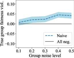
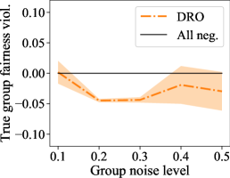
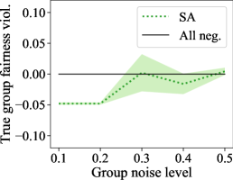
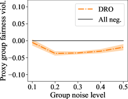
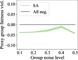
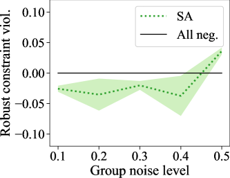
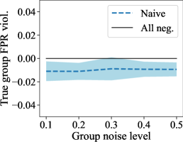
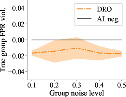
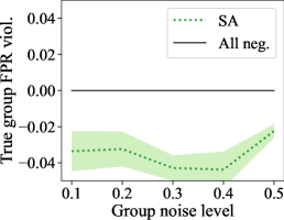
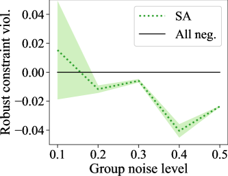
Figure 1: Case study 1 (Adult): maximum true group constraint violations on test set for the Naive, DRO, and soft assignments (SA) approaches for different group noise levels γ𝛾\gamma on the Adult dataset (mean and standard error over 10 train/val/test splits). The black solid line represents the performance of the trivial “all negatives” classifier, which has constraint violations of 0. A negative violation indicates satisfaction of the fairness constraints on the true groups.

Refer to caption Refer to caption Refer to caption

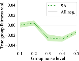
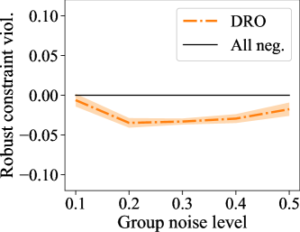
Figure 2: Case study 2 (Credit): maximum true group constraint violations on test set for the Naive, DRO, and soft assignments (SA) approaches for different group noise levels γ𝛾\gamma on the Credit dataset (mean and standard error over 10 train/val/test splits). This figure shows the max constraint violation over all TPR and FPR constraints, and Figure 6 in Appendix F.2 shows the breakdown of these constraint violations into the max TPR and the max FPR constraint violations.

Adult error rates Credit error rates Refer to caption Refer to caption
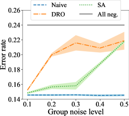
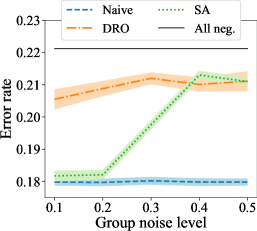
Figure 3: Error rates on test set for different group noise levels γ𝛾\gamma on the Adult dataset (left) and the Credit dataset (right) (mean and standard error over 10 train/val/test splits). The black solid line represents the performance of the trivial “all negatives” classifier. The soft assignments (SA) approach achieves lower error rates than DRO, and as the noise level increases, the gap in error rate between the naive approach and each robust approach increases.

7.3 Results

In case study 1 (Adult), the unconstrained model achieves an error rate of 0.1447±0.0012plus-or-minus0.14470.00120.1447\pm 0.0012 (mean and standard error over 10 splits) and a maximum constraint violation of 0.0234±0.0164plus-or-minus0.02340.01640.0234\pm 0.0164 on test set with respect to the true groups. The model that assumes knowledge of the true groups achieves an error rate of 0.1459±0.0012plus-or-minus0.14590.00120.1459\pm 0.0012 and a maximum constraint violation of 0.0469±0.0068plus-or-minus0.04690.0068-0.0469\pm 0.0068 on test set with respect to the true groups. As a sanity check, this demonstrates that when given access to the true groups, it is possible to satisfy the constraints on the test set with a reasonably low error rate.

In case study 2 (Credit), the unconstrained model achieves an error rate of 0.1797±0.0013plus-or-minus0.17970.00130.1797\pm 0.0013 (mean and standard error over 10 splits) and a maximum constraint violation of 0.0264±0.0071plus-or-minus0.02640.00710.0264\pm 0.0071 on the test set with respect to the true groups. The constrained model that assumes knowledge of the true groups achieves an error rate of 0.1796±0.0011plus-or-minus0.17960.00110.1796\pm 0.0011 and a maximum constraint violation of 0.0105±0.0070plus-or-minus0.01050.0070-0.0105\pm 0.0070 on the test set with respect to the true groups. For this dataset, it was possible to satisfy the constraints with approximately the same error rate on test as the unconstrained model. Note that the unconstrained model achieved a lower error rate on the train set than the constrained model (0.1792±0.0015plus-or-minus0.17920.00150.1792\pm 0.0015 unconstrained vs. 0.1798±0.0024plus-or-minus0.17980.00240.1798\pm 0.0024 constrained).

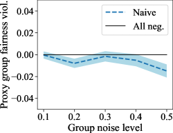
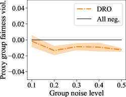
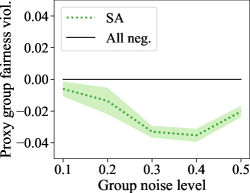
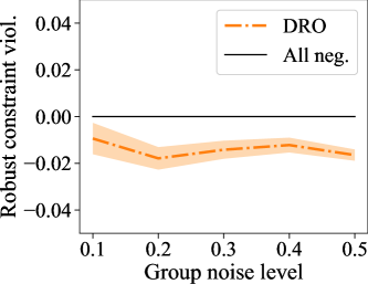
For both case studies, Figures 1 and 2 show that the robust approaches DRO (center) and soft group assignments (SA) (right) satisfy the constraints on average for all noise levels. As the noise level increases, the naïve approach (left) has increasingly higher true group constraint violations. The DRO and SA approaches come at a cost of a higher error rate than the naïve approach (Figure 3). The error rate of the naïve approach is close to the model optimized with constraints on the true groups G𝐺G, regardless of the noise level γ𝛾\gamma. However, as the noise increases, the naïve approach no longer controls the fairness violations on the true groups G𝐺G, even though it does satisfy the constraints on the noisy groups G^^𝐺\hat{G} (Figures 4 and 7 in Appendix F.2). DRO generally suffers from a higher error rate compared to SA (Figure 3), illustrating the conservatism of the DRO approach.

8 Conclusion

We explore the practical problem of enforcing group-based fairness for binary classification given noisy protected group information. In addition to providing new theoretical analysis of the naïve approach of only enforcing fairness on the noisy groups, we also propose two new robust approaches that guarantee satisfaction of the fairness criteria on the true groups. For the DRO approach, Lemma 1 gives a theoretical bound on the TV distance to use in the optimization problem. For the soft group assignments approach, we provide a theoretically ideal algorithm and a practical alternative algorithm for satisfying the robust fairness criteria proposed by Kallus et al. [37] while minimizing a training objective. We empirically show that both of these approaches managed to satisfy the constraints with respect to the true groups, even under difficult noise models.

In follow-up work, Narasimhan et al. [51] provide a general method for enforcing a large number of constraints at once, and enforce constraints concurrently on many possible realizations of noisy protected groups under a given noise model. This can be seen as an extension of the Soft Group Assignments approach that we propose in Section 6, which Narasimhan et al. [51] describe in their Appendix.

One additional avenue of future work is to empirically compare the robust approaches when the noisy groups have different dimensionality from the true groups (Appendix B.4). Second, the looseness of the bound in Lemma 1 can lead to over-conservatism of the DRO approach, suggesting a need to better calibrate the DRO neighborhood. Finally, it would be valuable to study the impact of distribution mismatch between the main dataset and the auxiliary dataset.

Broader Impact

As machine learning is increasingly employed in high stakes environments, any potential application has to be scrutinized to ensure that it will not perpetuate, exacerbate, or create new injustices. Aiming to make machine learning algorithms themselves intrinsically fairer, more inclusive, and more equitable plays an important role in achieving that goal. Group-based fairness [32, 25] is a popular approach that the machine learning community has used to define and evaluate fair machine learning algorithms. Until recently, such work has generally assumed access to clean, correct protected group labels in the data. Our work addresses the technical challenge of enforcing group-based fairness criteria under noisy, unreliable, or outdated group information. However, we emphasize that this technical improvement alone does not necessarily lead to an algorithm having positive societal impact, for reasons that we now delineate.

Choice of fairness criteria

First, our work does not address the choice of the group-based fairness criteria. Many different algorithmic fairness criteria have been proposed, with varying connections to prior sociopolitical framing [52, 35]. From an algorithmic standpoint, these different choices of fairness criteria have been shown to lead to very different prediction outcomes and tradeoffs [25]. Furthermore, even if a mathematical criterion may seem reasonable (e.g., equalizing positive prediction rates with demographic parity), Liu et al. [46] show that the long-term impacts may not always be desirable, and the choice of criteria should be heavily influenced by domain experts, along with awareness of tradeoffs.

Choice of protected groups

In addition to the specification of fairness criteria, our work also assumes that the true protected group labels have been pre-defined by the practitioner. However, in real applications, the selection of appropriate true protected group labels is itself a nontrivial issue.

First, the measurement and delineation of these protected groups should not be overlooked, as “the process of drawing boundaries around distinct social groups for fairness research is fraught; the construction of categories has a long history of political struggle and legal argumentation” [31]. Important considerations include the context in which the group labels were collected, who chose and collected them, and what implicit assumptions are being made by choosing these group labels. One example is the operationalization of race in the context of algorithmic fairness. Hanna et al. [31] critiques “treating race as an attribute, rather than a structural, institutional, and relational phenomenon.” The choice of categories surrounding gender identity and sexual orientation have strong implications and consequences as well [29], with entire fields dedicated to critiquing these constructs. Jacobs and Wallach [36] provide a general framework for understanding measurement issues for these sensitive attributes in the machine-learning setting, building on foundational work from the social sciences [5].

Another key consideration when defining protected groups is problems of intersectionality [15, 34]. Group-based fairness criteria inherently do not consider within-group inequality [38]. Even if we are able to enforce fairness criteria robustly for a given set of groups, the intersections of groups may still suffer [12].

Domain specific considerations

Finally, we emphasize that group-based fairness criteria simply may not be sufficient to mitigate problems of significant background injustice in certain domains. Abebe et al. [1] argue that computational methods have mixed roles in addressing social problems, where they can serve as diagnostics, formalizers, and rebuttals, and also that “computing acts as synecdoche when it makes long-standing social problems newly salient in the public eye.” Moreover, the use of the algorithm itself may perpetuate inequity, and in the case of credit scoring, create stratifying effects of economic classifications that shape life-chances [24]. We emphasize the importance of domain specific considerations ahead of time before applying any algorithmic solutions (even “fair” ones) in sensitive and impactful settings.

Acknowledgments and Disclosure of Funding

We thank Rediet Abebe, Timnit Gebru, and Margaret Mitchell for many useful pointers into the broader socio-technical literature that provides essential context for this work. We thank Jacob Steinhardt for helpful technical discussions. We also thank Stefania Albanesi and Domonkos Vámossy for an inspiring early discussion of practical scenarios when noisy protected groups occur. Finally, we thank Kush Bhatia, Collin Burns, Mihaela Curmei, Frances Ding, Sara Fridovich-Keil, Preetum Nakkiran, Adam Sealfon, and Alex Zhao for their helpful feedback on an early version of the paper. This material is based upon work supported by the National Science Foundation Graduate Research Fellowship Program under Grant No. DGE 1752814.

References

  • Abebe et al. [2020] Rediet Abebe, Solon Barocas, Jon Kleinberg, Karen Levy, Manish Raghavan, and David G Robinson. Roles for computing in social change. In Conference on Fairness, Accountability, and Transparency (FAccT), 2020.
  • Agarwal et al. [2018] Alekh Agarwal, Alina Beygelzimer, Miroslav Dudík, John Langford, and Hanna Wallach. A reductions approach to fair classification. In International Conference on Machine Learning (ICML), 2018.
  • Aghaei et al. [2019] Sina Aghaei, Mohammad Javad Azizi, and Phebe Vayanos. Learning optimal and fair decision trees for non-discriminative decision-making. In AAAI Conference on Artificial Intelligence, volume 33, pages 1418–1426, 2019.
  • Awasthi et al. [2020] Pranjal Awasthi, Matthäus Kleindessner, and Jamie Morgenstern. Equalized odds postprocessing under imperfect group information. In Conference on Artificial Intelligence and Statistics (AISTATS), 2020.
  • Bandalos [2017] Deborah L. Bandalos. Measurement Theory and Applications for the Social Sciences. Guilford Publications, 2017.
  • Barocas et al. [2019] Solon Barocas, Moritz Hardt, and Arvind Narayanan. Fairness and Machine Learning. fairmlbook.org, 2019. http://www.fairmlbook.org.
  • Ben-Tal et al. [2009] Aharon Ben-Tal, Laurent El Ghaoui, and Arkadi Nemirovski. Robust Optimization. Princeton Series in Applied Mathematics. Princeton University Press, October 2009.
  • Ben-Tal et al. [2013] Aharon Ben-Tal, Dick Den Hertog, Anja De Waegenaere, Bertrand Melenberg, and Gijs Rennen. Robust solutions of optimization problems affected by uncertain probabilities. Management Science, 59(2):341–357, 2013.
  • Bera et al. [2019] Suman Bera, Deeparnab Chakrabarty, Nicolas Flores, and Maryam Negahbani. Fair algorithms for clustering. In Advances in Neural Information Processing Systems (NeurIPS), pages 4954–4965, 2019.
  • Berk et al. [2017] Richard Berk, Hoda Heidari, Shahin Jabbari, Matthew Joseph, Michael Kearns, Jamie Morgenstern, Seth Neel, and Aaron Roth. A convex framework for fair regression. arXiv preprint arXiv:1706.02409, 2017.
  • Bertsimas et al. [2011] Dimitris Bertsimas, David B Brown, and Constantine Caramanis. Theory and applications of robust optimization. SIAM Review, 53(3):464–501, 2011.
  • Buolamwini and Gebru [2018] Joy Buolamwini and Timnit Gebru. Gender shades: Intersectional accuracy disparities in commercial gender classification. In Journal of Machine Learning Research (JMLR), 2018.
  • Cotter et al. [2019a] A. Cotter, H. Jiang, and K. Sridharan. Two-player games for efficient non-convex constrained optimization. In International Conference on Algorithmic Learning Theory (ALT), 2019a.
  • Cotter et al. [2019b] Andrew Cotter, Heinrich Jiang, Serena Wang, Taman Narayan, Seungil You, Karthik Sridharan, and Maya R. Gupta. Optimization with non-differentiable constraints with applications to fairness, recall, churn, and other goals. Journal of Machine Learning Research (JMLR), 20(172):1–59, 2019b.
  • Crenshaw [1990] Kimberle Crenshaw. Mapping the margins: Intersectionality, identity politics, and violence against women of color. Stanford Law Review, 43:1241, 1990.
  • Davenport et al. [2010] Mark A. Davenport, Richard G. Baraniuk, and Clayton D. Scott. Tuning support vector machines for minimax and Neyman-Pearson classification. IEEE Transactions on Pattern Analysis and Machine Intelligence, 2010.
  • Donini et al. [2018] Michele Donini, Luca Oneto, Shai Ben-David, John Shawe-Taylor, and Massimiliano Pontil. Empirical risk minimization under fairness constraints. In Advances in Neural Information Processing Systems (NeurIPS), 2018.
  • Dua and Graff [2017] Dheeru Dua and Casey Graff. UCI machine learning repository, 2017. URL http://archive.ics.uci.edu/ml.
  • Duchi and Namkoong [2018] John Duchi and Hongseok Namkoong. Learning models with uniform performance via distributionally robust optimization. arXiv preprint arXiv:1810.08750, 2018.
  • Duchi et al. [2008] John Duchi, Shai Shalev-Shwartz, Yoram Singer, and Tushar Chandra. Efficient projections onto the 1subscript1\ell_{1}-ball for learning in high dimensions. In International Conference on Machine Learning (ICML), 2008.
  • Dwork et al. [2012] Cynthia Dwork, Moritz Hardt, Toniann Pitassi, Omer Reingold, and Rich Zemel. Fairness through awareness. In Innovations in Theoretical Computer Science (ITCS), pages 214–226. ACM, 2012.
  • Eban et al. [2017] Elad Eban, Mariano Schain, Alan Mackey, Ariel Gordon, Rif A. Saurous, and Gal Elidan. Scalable learning of non-decomposable objectives. In International Conference on Artificial Intelligence and Statistics (AISTATS), 2017.
  • Esfahani and Kuhn. [2018] P. M. Esfahani and D. Kuhn. Data-driven distributionally robust optimization using the Wasserstein metric: Performance guarantees and tractable reformulations. Mathematical Programming, 171:115–166, 2018.
  • Fourcade and Healy [2013] Marion Fourcade and Kieran Healy. Classification situations: Life-chances in the neoliberal era. Accounting, Organizations and Society, 38(8):559–572, 2013.
  • Friedler et al. [2019] Sorelle A. Friedler, Carlos Scheidegger, Suresh Venkatasubramanian, Sonam Choudhary, Evan P. Hamilton, and Derek Roth. A comparative study of fairness-enhancing interventions in machine learning. In Conference on Fairness, Accountability, and Transparency (FAccT), 2019.
  • Gillis [2020] Talia B Gillis. False dreams of algorithmic fairness: The case of credit pricing. Available at SSRN 3571266, 2020.
  • Goh et al. [2016] Gabriel Goh, Andrew Cotter, Maya Gupta, and Michael Friedlander. Satisfying real-world goals with dataset constraints. In Advances in Neural Information Processing Systems (NeurIPS), 2016.
  • Grari et al. [2020] Vincent Grari, Boris Ruf, Sylvain Lamprier, and Marcin Detyniecki. Achieving fairness with decision trees: An adversarial approach. Data Science and Engineering, 5(2):99–110, 2020.
  • Group [2014] The GenIUSS Group. Best Practices for Asking Questions to Identify Transgender and Other Gender Minority Respondents on Population-Based Surveys. The Williams Institute, 2014.
  • Gupta et al. [2018] Maya Gupta, Andrew Cotter, Mahdi Milani Fard, and Serena Wang. Proxy fairness. arXiv preprint arXiv:1806.11212, 2018.
  • Hanna et al. [2020] Alex Hanna, Emily Denton, Andrew Smart, and Jamila Smith-Loud. Towards a critical race methodology in algorithmic fairness. Conference on Fairness, Accountability, and Transparency (FAccT), 2020.
  • Hardt et al. [2016] Moritz Hardt, Eric Price, and Nathan Srebro. Equality of opportunity in supervised learning. In Advances in Neural Information Processing Systems (NeurIPS), 2016.
  • Hashimoto et al. [2018] Tatsunori B. Hashimoto, Megha Srivastava, Hongseok Namkoong, and Percy Liang. Fairness without demographics in repeated loss minimization. In International Conference on Machine Learning (ICML), 2018.
  • Hooks [1992] Bell Hooks. Yearning: Race, gender, and cultural politics. 1992.
  • Hutchinson and Mitchell [2019] Ben Hutchinson and M. Mitchell. 50 years of test (un)fairness: Lessons for machine learning. In Conference on Fairness, Accountability, and Transparency (FAccT), 2019.
  • Jacobs and Wallach [2019] Abigail Z. Jacobs and Hanna Wallach. Measurement and fairness. arXiv preprint arXiv:1912.05511, 2019.
  • Kallus et al. [2020] Nathan Kallus, Xiaojie Mao, and Angela Zhou. Assessing algorithmic fairness with unobserved protected class using data combination. Conference on Fairness, Accountability, and Transparency (FAccT), 2020.
  • Kasy and Abebe [2020] Maximilian Kasy and Rediet Abebe. Fairness, equality, and power in algorithmic decision-making. ICML Workshop on Participatory Approaches to Machine Learning, 2020.
  • Kolodny [2019] Niko Kolodny. Why equality of treatment and opportunity might matter. Philosophical Studies, 176:3357–3366, 2019.
  • Krumpal [2011] Ivar Krumpal. Determinants of social desirability bias in sensitive surveys: a literature review. Quality and Quantity, 47:2025–2047, 2011.
  • Kusner et al. [2017] Matt J. Kusner, Joshua R. Loftus, Chris Russell, and Ricardo Silva. Counterfactual fairness. In Advances in Neural Information Processing Systems (NeurIPS), 2017.
  • Lahoti et al. [2020] Preethi Lahoti, Alex Beutel, Jilin Chen, Kang Lee, Flavien Prost, Nithum Thain, Xuezhi Wang, and Ed H Chi. Fairness without demographics through adversarially reweighted learning. arXiv preprint arXiv:2006.13114, 2020.
  • Lamy et al. [2019] Alexandre Lamy, Ziyuan Zhong, Aditya Krishna Menon, and Nakul Verma. Noise-tolerant fair classification. In Advances in Neural Information Processing Systems (NeurIPS), 2019.
  • Lazar and Vijaykumar [2020] Claire Lazar and Suhas Vijaykumar. A resolution in algorithmic fairness: Calibrated scores for fair classifications. arXiv preprint arXiv:2002.07676, 2020.
  • Li et al. [2019] Jiajin Li, Sen Huang, and Anthony Man-Cho So. A first-order algorithmic framework for Wasserstein distributionally robust logistic regression. In Advances in Neural Information Processing Systems (NeurIPS), 2019.
  • Liu et al. [2018] Lydia T. Liu, Sarah Dean, Esther Rolf, Max Simchowitz, and Moritz Hardt. Delayed impact of fair machine learning. In International Conference on Machine Learning (ICML), 2018.
  • Mozannar et al. [2020] Hussein Mozannar, Mesrob I Ohannessian, and Nathan Srebro. Fair learning with private demographic data. arXiv preprint arXiv:2002.11651, 2020.
  • Namkoong and Duchi [2016] Hongseok Namkoong and John Duchi. Stochastic gradient methods for distributionally robust optimization with f-divergences. In Advances in Neural Information Processing Systems (NeurIPS), 2016.
  • Narasimhan et al. [2019a] Harikrishna Narasimhan, Andrew Cotter, and Maya Gupta. Optimizing generalized rate metrics with three players. In Advances in Neural Information Processing Systems (NeurIPS), 2019a.
  • Narasimhan et al. [2019b] Harikrishna Narasimhan, Andrew Cotter, and Maya R. Gupta. On making stochastic classifiers deterministic. In Advances in Neural Information Processing Systems (NeurIPS), 2019b.
  • Narasimhan et al. [2020] Harikrishna Narasimhan, Andrew Cotter, Yichen Zhou, Serena Wang, and Wenshuo Guo. Approximate heavily-constrained learning with lagrange multiplier models. In Advances in Neural Information Processing Systems (NeurIPS), 2020.
  • Narayanan [2018] Arvind Narayanan. Translation tutorial: 21 fairness definitions and their politics. In Conference on Fairness, Accountability, and Transparency (FAccT), 2018.
  • Russell et al. [2017] Chris Russell, Matt J. Kusner, Joshua Loftus, and Ricardo Silva. When worlds collide: Integrating different counterfactual assumptions in fairness. In Advances in Neural Information Processing Systems (NeurIPS), 2017.
  • Villani [2009] Cédric Villani. Optimal Transport, Old and New, volume 338 of Grundlehren der Mathematischen Wissenschaften. Springer-Verlag, 2009.
  • Wang and Gupta [2020] Serena Wang and Maya R. Gupta. Deontological ethics by monotonicity shape constraints. In International Conference on Artificial Intelligence and Statistics (AISTATS), 2020.
  • Woodworth et al. [2017] Blake Woodworth, Suriya Gunasekar, Mesrob I. Ohannessian, and Nathan Srebro. Learning non-discriminatory predictors. In Conference on Learning Theory (COLT), pages 1920–1953, 2017.
  • Yeh and hui Lien [2009] I-Cheng Yeh and Che hui Lien. The comparisons of data mining techniques for the predictive accuracy of probability of default of credit card clients. Expert Systems with Applications, 36:2473–2480, 2009.
  • Zafar et al. [2017] Muhammad Bilal Zafar, Isabel Valera, Manuel Gomez Rodriguez, and Krishna P. Gummadi. Fairness constraints: Mechanisms for fair classification. In International Conference on Artificial Intelligence and Statistics (AISTATS), 2017.
  • Zafar et al. [2019] Muhammad Bilal Zafar, Isabel Valera, Manuel Gomez-Rodriguez, and Krishna P. Gummadi. Fairness constraints: A flexible approach for fair classification. Journal of Machine Learning Research (JMLR), 20:1–42, 2019.

Appendix A Proofs for Section 4

This section provides proofs and definitions details for the theorems and lemmas presented in Section 4.

A.1 Proofs for TV distance

Definition 1.

(TV distance) Let c(x,y)=𝟙(xy)𝑐𝑥𝑦1𝑥𝑦c(x,y)=\operatorname{\mathbbm{1}}(x\neq y) be a metric, and let π𝜋\pi be a coupling between probability distributions p𝑝p and q𝑞q. Define the total variation (TV) distance between two distributions p,q𝑝𝑞p,q as

TV(p,q)𝑇𝑉𝑝𝑞\displaystyle TV(p,q) =infπ𝔼X,Yπ[c(X,Y)]absentsubscriptinfimum𝜋subscript𝔼similar-to𝑋𝑌𝜋delimited-[]𝑐𝑋𝑌\displaystyle=\inf_{\pi}\mathbb{E}_{X,Y\sim\pi}[c(X,Y)]
s.t.π(x,y)𝑑y=p(x),π(x,y)𝑑x=q(y).formulae-sequences.t.𝜋𝑥𝑦differential-d𝑦𝑝𝑥𝜋𝑥𝑦differential-d𝑥𝑞𝑦\displaystyle\text{s.t.}\int\pi(x,y)dy=p(x),\int\pi(x,y)dx=q(y).
Theorem 1.

Suppose a model with parameters θ𝜃\theta satisfies fairness criteria with respect to the noisy groups G^^𝐺\hat{G}:

g^j(θ)0j𝒢.subscript^𝑔𝑗𝜃0for-all𝑗𝒢\hat{g}_{j}(\theta)\leq 0\;\;\forall j\in\mathcal{G}.

Suppose |h(θ,x1,y1)h(θ,x2,y2)|1𝜃subscript𝑥1subscript𝑦1𝜃subscript𝑥2subscript𝑦21|h(\theta,x_{1},y_{1})-h(\theta,x_{2},y_{2})|\leq 1 for any (x1,y1)(x2,y2)subscript𝑥1subscript𝑦1subscript𝑥2subscript𝑦2(x_{1},y_{1})\neq(x_{2},y_{2}). If TV(pj,p^j)γj𝑇𝑉subscript𝑝𝑗subscript^𝑝𝑗subscript𝛾𝑗TV(p_{j},\hat{p}_{j})\leq\gamma_{j} for all j𝒢𝑗𝒢j\in\mathcal{G}, then the fairness criteria with respect to the true groups G𝐺G will be satisfied within slacks γjsubscript𝛾𝑗\gamma_{j} for each group:

gj(θ)γjj𝒢.formulae-sequencesubscript𝑔𝑗𝜃subscript𝛾𝑗for-all𝑗𝒢g_{j}(\theta)\leq\gamma_{j}\quad\forall j\in\mathcal{G}.
Proof.

For any group label j𝑗j,

gj(θ)=gj(θ)g^j(θ)+g^j(θ)|gj(θ)g^j(θ)|+g^j(θ).subscript𝑔𝑗𝜃subscript𝑔𝑗𝜃subscript^𝑔𝑗𝜃subscript^𝑔𝑗𝜃subscript𝑔𝑗𝜃subscript^𝑔𝑗𝜃subscript^𝑔𝑗𝜃\displaystyle g_{j}(\theta)=g_{j}(\theta)-\hat{g}_{j}(\theta)+\hat{g}_{j}(\theta)\leq|g_{j}(\theta)-\hat{g}_{j}(\theta)|+\hat{g}_{j}(\theta).

By Kantorovich-Rubenstein theorem (provided here as Theorem 2), we also have

|g^j(θ)gj(θ)|subscript^𝑔𝑗𝜃subscript𝑔𝑗𝜃\displaystyle|\hat{g}_{j}(\theta)-g_{j}(\theta)| =|𝔼X,Yp^j[h(θ,X,Y)]𝔼X,Ypj[h(θ,X,Y)]|TV(pj,p^j).absentsubscript𝔼similar-to𝑋𝑌subscript^𝑝𝑗delimited-[]𝜃𝑋𝑌subscript𝔼similar-to𝑋𝑌subscript𝑝𝑗delimited-[]𝜃𝑋𝑌𝑇𝑉subscript𝑝𝑗subscript^𝑝𝑗\displaystyle=|\mathbb{E}_{X,Y\sim\hat{p}_{j}}[h(\theta,X,Y)]-\mathbb{E}_{X,Y\sim p_{j}}[h(\theta,X,Y)]|\leq TV(p_{j},\hat{p}_{j}).

By assumption that θ𝜃\theta satisifes fairness constraints with respect to the noisy groups G^^𝐺\hat{G}, g^j(θ)0subscript^𝑔𝑗𝜃0\hat{g}_{j}(\theta)\leq 0. Thus, we have the desired result that gj(θ)TV(pj,p^j)γjsubscript𝑔𝑗𝜃𝑇𝑉subscript𝑝𝑗subscript^𝑝𝑗subscript𝛾𝑗g_{j}(\theta)\leq TV(p_{j},\hat{p}_{j})\leq\gamma_{j}.

Note that if pjsubscript𝑝𝑗p_{j} and p^jsubscript^𝑝𝑗\hat{p}_{j} are discrete, then the TV distance TV(pj,pj^)𝑇𝑉subscript𝑝𝑗^subscript𝑝𝑗TV(p_{j},\hat{p_{j}}) could be very large. In that case, the bound would still hold, but would be loose. ∎

Theorem 2.

(Kantorovich-Rubinstein).111Edwards, D.A. On the Kantorovich–Rubinstein theorem. Expositiones Mathematicae, 20(4):387-398, 2011. Call a function f𝑓f Lipschitz in c𝑐c if |f(x)f(y)|c(x,y)𝑓𝑥𝑓𝑦𝑐𝑥𝑦|f(x)-f(y)|\leq c(x,y) for all x,y𝑥𝑦x,y, and let (c)𝑐\mathcal{L}(c) denote the space of such functions. If c𝑐c is a metric, then we have

Wc(p,q)=supf(c)𝔼Xp[f(X)]𝔼Xq[f(X)].subscript𝑊𝑐𝑝𝑞subscriptsupremum𝑓𝑐subscript𝔼similar-to𝑋𝑝delimited-[]𝑓𝑋subscript𝔼similar-to𝑋𝑞delimited-[]𝑓𝑋W_{c}(p,q)=\sup_{f\in\mathcal{L}(c)}\mathbb{E}_{X\sim p}[f(X)]-\mathbb{E}_{X\sim q}[f(X)].

As a special case, take c(x,y)=𝕀(xy)𝑐𝑥𝑦𝕀𝑥𝑦c(x,y)=\mathbb{I}(x\neq y) (corresponding to TV distance). Then f(c)𝑓𝑐f\in\mathcal{L}(c) if and only if |f(x)f(y)|1𝑓𝑥𝑓𝑦1|f(x)-f(y)|\leq 1 for all xy𝑥𝑦x\neq y. By translating f𝑓f, we can equivalently take the supremum over all f𝑓f mapping to [0,1]01[0,1]. This says that

TV(p,q)=supf:𝒳[0,1]𝔼Xp[f(X)]𝔼Xq[f(X)]𝑇𝑉𝑝𝑞subscriptsupremum:𝑓𝒳01subscript𝔼similar-to𝑋𝑝delimited-[]𝑓𝑋subscript𝔼similar-to𝑋𝑞delimited-[]𝑓𝑋TV(p,q)=\sup_{f:\mathcal{X}\to[0,1]}\mathbb{E}_{X\sim p}[f(X)]-\mathbb{E}_{X\sim q}[f(X)]
Lemma 1.

Suppose P(G=i)=P(G^=i)𝑃𝐺𝑖𝑃^𝐺𝑖P(G=i)=P(\hat{G}=i) for a given i{1,2,,m}𝑖12𝑚i\in\{1,2,...,m\}. Then TV(pi,p^i)P(GG^|G=i)𝑇𝑉subscript𝑝𝑖subscript^𝑝𝑖𝑃𝐺conditional^𝐺𝐺𝑖TV(p_{i},\hat{p}_{i})\leq P(G\neq\hat{G}|G=i).

Proof.

For probability measures pisubscript𝑝𝑖p_{i} and p^isubscript^𝑝𝑖\hat{p}_{i}, the TV distance is given by

TV(pi,p^i)=sup{|pi(A)p^i(A)|:A is a measurable event}.TV(p_{i},\hat{p}_{i})=\sup\{|p_{i}(A)-\hat{p}_{i}(A)|:A\text{ is a measurable event}\}.

Fix A𝐴A to be any measurable event for both pisubscript𝑝𝑖p_{i} and p^isubscript^𝑝𝑖\hat{p}_{i}. This means that A𝐴A is also a measurable event for p𝑝p, the distribution of the random variables X,Y𝑋𝑌X,Y. By definition of pisubscript𝑝𝑖p_{i}, pi(A)=P(A|G=i)subscript𝑝𝑖𝐴𝑃conditional𝐴𝐺𝑖p_{i}(A)=P(A|G=i). Then

|pi(A)p^i(A)|subscript𝑝𝑖𝐴subscript^𝑝𝑖𝐴\displaystyle|p_{i}(A)-\hat{p}_{i}(A)| =|P(A|G=i)P(A|G^=i)|\displaystyle=|P(A|G=i)-P(A|\hat{G}=i)|
=|P(A|G=i,G^=i)P(G^=i|G=i)\displaystyle=|P(A|G=i,\hat{G}=i)P(\hat{G}=i|G=i)
+P(A|G=i,G^i)P(G^i|G=i)𝑃formulae-sequenceconditional𝐴𝐺𝑖^𝐺𝑖𝑃^𝐺conditional𝑖𝐺𝑖\displaystyle\quad+P(A|G=i,\hat{G}\neq i)P(\hat{G}\neq i|G=i)
P(A|G^=i,G=i)P(G=i|G^=i)𝑃formulae-sequenceconditional𝐴^𝐺𝑖𝐺𝑖𝑃𝐺conditional𝑖^𝐺𝑖\displaystyle\quad-P(A|\hat{G}=i,G=i)P(G=i|\hat{G}=i)
P(A|G^=i,Gi)P(Gi|G^=i)|\displaystyle\quad-P(A|\hat{G}=i,G\neq i)P(G\neq i|\hat{G}=i)|
=|P(A|G=i,G^=i)(P(G^=i|G=i)P(G=i|G^=i))\displaystyle=|P(A|G=i,\hat{G}=i)\left(P(\hat{G}=i|G=i)-P(G=i|\hat{G}=i)\right)
P(G^G|G=i)(P(A|G=i,G^i)P(A|G^=i,Gi))|\displaystyle\quad-P(\hat{G}\neq G|G=i)\left(P(A|G=i,\hat{G}\neq i)-P(A|\hat{G}=i,G\neq i)\right)|
=|0P(G^G|G=i)(P(A|G=i,G^i)P(A|G^=i,Gi))|\displaystyle=|0-P(\hat{G}\neq G|G=i)\left(P(A|G=i,\hat{G}\neq i)-P(A|\hat{G}=i,G\neq i)\right)|
P(G^G|G=i)absent𝑃^𝐺conditional𝐺𝐺𝑖\displaystyle\leq P(\hat{G}\neq G|G=i)

The second equality follows from the law of total probability. The third and the fourth equalities follow from the assumption that P(G=i)=P(G^=i)𝑃𝐺𝑖𝑃^𝐺𝑖P(G=i)=P(\hat{G}=i), which implies that P(G^=G|G=i)=P(G=G^|G^=i)𝑃^𝐺conditional𝐺𝐺𝑖𝑃𝐺conditional^𝐺^𝐺𝑖P(\hat{G}=G|G=i)=P(G=\hat{G}|\hat{G}=i) since

P(G=G^|G=i)=P(G=G^,G=i)P(G=i)=P(G=G^,G^=i)P(G^=i)=P(G=G^|G^=i).𝑃𝐺conditional^𝐺𝐺𝑖𝑃formulae-sequence𝐺^𝐺𝐺𝑖𝑃𝐺𝑖𝑃formulae-sequence𝐺^𝐺^𝐺𝑖𝑃^𝐺𝑖𝑃𝐺conditional^𝐺^𝐺𝑖P(G=\hat{G}|G=i)=\frac{P(G=\hat{G},G=i)}{P(G=i)}=\frac{P(G=\hat{G},\hat{G}=i)}{P(\hat{G}=i)}=P(G=\hat{G}|\hat{G}=i).

This further implies that P(G^i|G=i)=P(Gi|G^=i)𝑃^𝐺conditional𝑖𝐺𝑖𝑃𝐺conditional𝑖^𝐺𝑖P(\hat{G}\neq i|G=i)=P(G\neq i|\hat{G}=i).

Since |pi(A)p^i(A)|P(G^G|G=i)subscript𝑝𝑖𝐴subscript^𝑝𝑖𝐴𝑃^𝐺conditional𝐺𝐺𝑖|p_{i}(A)-\hat{p}_{i}(A)|\leq P(\hat{G}\neq G|G=i) for any measurable event A𝐴A, the supremum over all events A𝐴A is also bounded by P(G^G|G=i)𝑃^𝐺conditional𝐺𝐺𝑖P(\hat{G}\neq G|G=i). This gives the desired bound on the TV distance. ∎

A.2 Generalization to Wasserstein distances

Theorem 1 can be directly extended to loss functions that are Lipschitz in other metrics. To do so, we first provide a more general definition of Wasserstein distances:

Definition 2.

(Wasserstein distance) Let c(x,y)𝑐𝑥𝑦c(x,y) be a metric, and let π𝜋\pi be a coupling between p𝑝p and q𝑞q. Define the Wasserstein distance between two distributions p,q𝑝𝑞p,q as

Wc(p,q)=infπsubscript𝑊𝑐𝑝𝑞subscriptinfimum𝜋\displaystyle W_{c}(p,q)=\inf_{\pi}\;\; 𝔼X,Yπ[c(X,Y)]subscript𝔼similar-to𝑋𝑌𝜋delimited-[]𝑐𝑋𝑌\displaystyle\mathbb{E}_{X,Y\sim\pi}[c(X,Y)]
s.t. π(x,y)𝑑y=p(x),π(x,y)𝑑x=q(y).formulae-sequence𝜋𝑥𝑦differential-d𝑦𝑝𝑥𝜋𝑥𝑦differential-d𝑥𝑞𝑦\displaystyle\int\pi(x,y)dy=p(x),\int\pi(x,y)dx=q(y).

As a familiar example, if c(x,y)=xy2𝑐𝑥𝑦subscriptnorm𝑥𝑦2c(x,y)=||x-y||_{2}, then Wcsubscript𝑊𝑐W_{c} is the earth-mover distance, and (c)𝑐\mathcal{L}(c) is the class of 1-Lipschitz functions. Using the Wasserstein distance Wcsubscript𝑊𝑐W_{c} under different metrics c𝑐c, we can bound the fairness violations for constraint functions hh beyond those specified for the TV distance in Theorem 1.

Theorem 3.

Suppose a model with parameters θ𝜃\theta satisfies fairness criteria with respect to the noisy groups G^^𝐺\hat{G}:

g^j(θ)0j𝒢.subscript^𝑔𝑗𝜃0for-all𝑗𝒢\hat{g}_{j}(\theta)\leq 0\;\;\forall j\in\mathcal{G}.

Suppose the function hh satisfies |h(θ,x1,y1)h(θ,x2,y2)|c((x1,y1),(x2,y2))𝜃subscript𝑥1subscript𝑦1𝜃subscript𝑥2subscript𝑦2𝑐subscript𝑥1subscript𝑦1subscript𝑥2subscript𝑦2|h(\theta,x_{1},y_{1})-h(\theta,x_{2},y_{2})|\leq c((x_{1},y_{1}),(x_{2},y_{2})) for any (x1,y1)(x2,y2)subscript𝑥1subscript𝑦1subscript𝑥2subscript𝑦2(x_{1},y_{1})\neq(x_{2},y_{2}) w.r.t a metric c𝑐c. If Wc(pj,p^j)γjsubscript𝑊𝑐subscript𝑝𝑗subscript^𝑝𝑗subscript𝛾𝑗W_{c}(p_{j},\hat{p}_{j})\leq\gamma_{j} for all j𝒢𝑗𝒢j\in\mathcal{G}, then the fairness criteria with respect to the true groups G𝐺G will be satisfied within slacks γjsubscript𝛾𝑗\gamma_{j} for each group:

gj(θ)γjj𝒢.formulae-sequencesubscript𝑔𝑗𝜃subscript𝛾𝑗for-all𝑗𝒢g_{j}(\theta)\leq\gamma_{j}\quad\forall j\in\mathcal{G}.
Proof.

By the triangle inequality, for any group label j𝑗j,

|gj(θ)g(θ)||gj(θ)g^j(θ)|+g^j(θ)subscript𝑔𝑗𝜃𝑔𝜃subscript𝑔𝑗𝜃subscript^𝑔𝑗𝜃subscript^𝑔𝑗𝜃\displaystyle|g_{j}(\theta)-g(\theta)|\leq|g_{j}(\theta)-\hat{g}_{j}(\theta)|+\hat{g}_{j}(\theta)

By Kantorovich-Rubenstein theorem (provided here as Theorem 2), we also have

|g^j(θ)gj(θ)|subscript^𝑔𝑗𝜃subscript𝑔𝑗𝜃\displaystyle|\hat{g}_{j}(\theta)-g_{j}(\theta)| =|𝔼X,Yp^j[h(θ,X,Y)]𝔼X,Ypj[h(θ,X,Y)]|absentsubscript𝔼similar-to𝑋𝑌subscript^𝑝𝑗delimited-[]𝜃𝑋𝑌subscript𝔼similar-to𝑋𝑌subscript𝑝𝑗delimited-[]𝜃𝑋𝑌\displaystyle=|\mathbb{E}_{X,Y\sim\hat{p}_{j}}[h(\theta,X,Y)]-\mathbb{E}_{X,Y\sim p_{j}}[h(\theta,X,Y)]|
Wc(pj,p^j).absentsubscript𝑊𝑐subscript𝑝𝑗subscript^𝑝𝑗\displaystyle\leq W_{c}(p_{j},\hat{p}_{j}).

By the assumption that θ𝜃\theta satisifes fairness constraints with respect to the noisy groups G^^𝐺\hat{G}, g^j(θ)0subscript^𝑔𝑗𝜃0\hat{g}_{j}(\theta)\leq 0. Therefore, combining these with the triangle inequality, we get the desired result. ∎

Appendix B Details on DRO formulation for TV distance

Here we describe the details on solving the DRO problem (3) with TV distance using the empirical Lagrangian formulation. We also provide the pseudocode we used for the projected gradient-based algorithm to solve it.

B.1 Empirical Lagrangian Formulation

We rewrite the constrained optimization problem (3) as a minimax problem using the Lagrangian formulation. We also convert all expectations into expectations over empirical distributions given a dataset of n𝑛n samples (X1,Y1,G1),,(Xn,Yn,Gn)subscript𝑋1subscript𝑌1subscript𝐺1subscript𝑋𝑛subscript𝑌𝑛subscript𝐺𝑛(X_{1},Y_{1},G_{1}),...,(X_{n},Y_{n},G_{n}).

Let njsubscript𝑛𝑗n_{j} denote the number of samples that belong to a true group G=j𝐺𝑗G=j. Let the empirical distribution p^jnsubscript^𝑝𝑗superscript𝑛\hat{p}_{j}\in\mathbb{R}^{n} be a vector with i𝑖i-th entry p^ji=1njsuperscriptsubscript^𝑝𝑗𝑖1subscript𝑛𝑗\hat{p}_{j}^{i}=\frac{1}{n_{j}} if the i𝑖i-th example has a noisy group membership G^i=jsubscript^𝐺𝑖𝑗\hat{G}_{i}=j, and 00 otherwise. Replacing all expectations with expectations over the appropriate empirical distributions, the empirical form of (3) can be written as:

minθ1ni=1nl(θ,Xi,Yi)s.t.maxp~j𝔹γj(p^j)i=1np~jih(θ,Xi,Yi)0j𝒢formulae-sequencesubscript𝜃1𝑛superscriptsubscript𝑖1𝑛𝑙𝜃subscript𝑋𝑖subscript𝑌𝑖s.t.subscriptsubscript~𝑝𝑗subscript𝔹subscript𝛾𝑗subscript^𝑝𝑗superscriptsubscript𝑖1𝑛superscriptsubscript~𝑝𝑗𝑖𝜃subscript𝑋𝑖subscript𝑌𝑖0for-all𝑗𝒢\displaystyle\begin{split}\min_{\theta}\quad&\frac{1}{n}\sum_{i=1}^{n}l(\theta,X_{i},Y_{i})\\ \text{s.t.}\quad&\max_{\tilde{p}_{j}\in\mathbb{B}_{\gamma_{j}}(\hat{p}_{j})}\sum_{i=1}^{n}\tilde{p}_{j}^{i}h(\theta,X_{i},Y_{i})\leq 0\quad\forall j\in\mathcal{G}\end{split} (9)

where 𝔹γj(p^j)={p~jn:12i=1n|p~jip^ji|γj,i=1np~ji=1,p~ji0i=1,,n}subscript𝔹subscript𝛾𝑗subscript^𝑝𝑗conditional-setsubscript~𝑝𝑗superscript𝑛formulae-sequence12superscriptsubscript𝑖1𝑛superscriptsubscript~𝑝𝑗𝑖superscriptsubscript^𝑝𝑗𝑖subscript𝛾𝑗formulae-sequencesuperscriptsubscript𝑖1𝑛superscriptsubscript~𝑝𝑗𝑖1formulae-sequencesuperscriptsubscript~𝑝𝑗𝑖0for-all𝑖1𝑛\mathbb{B}_{\gamma_{j}}(\hat{p}_{j})=\{\tilde{p}_{j}\in\mathbb{R}^{n}:\frac{1}{2}\sum_{i=1}^{n}|\tilde{p}_{j}^{i}-\hat{p}_{j}^{i}|\leq\gamma_{j},\sum_{i=1}^{n}\tilde{p}_{j}^{i}=1,\tilde{p}_{j}^{i}\geq 0\quad\forall i=1,...,n\}.

For ease of notation, for j{1,2,,m}𝑗12𝑚j\in\{1,2,...,m\}, let

f(θ)=1ni=1nl(θ,Xi,Yi)𝑓𝜃1𝑛superscriptsubscript𝑖1𝑛𝑙𝜃subscript𝑋𝑖subscript𝑌𝑖f(\theta)=\frac{1}{n}\sum_{i=1}^{n}l(\theta,X_{i},Y_{i})
fj(θ,p~j)=i=1np~jih(θ,Xi,Yi).subscript𝑓𝑗𝜃subscript~𝑝𝑗superscriptsubscript𝑖1𝑛superscriptsubscript~𝑝𝑗𝑖𝜃subscript𝑋𝑖subscript𝑌𝑖f_{j}(\theta,\tilde{p}_{j})=\sum_{i=1}^{n}\tilde{p}_{j}^{i}h(\theta,X_{i},Y_{i}).

Then the Lagrangian of the empirical formulation (9) is

(θ,λ)=f(θ)+j=1mλjmaxp~j𝔹γ(p^j)fj(θ,p~j)𝜃𝜆𝑓𝜃superscriptsubscript𝑗1𝑚subscript𝜆𝑗subscriptsubscript~𝑝𝑗subscript𝔹𝛾subscript^𝑝𝑗subscript𝑓𝑗𝜃subscript~𝑝𝑗\mathcal{L}(\theta,\lambda)=f(\theta)+\sum_{j=1}^{m}\lambda_{j}\max_{\tilde{p}_{j}\in\mathbb{B}_{\gamma}(\hat{p}_{j})}f_{j}(\theta,\tilde{p}_{j})

and problem (9) can be rewritten as

minθmaxλ0f(θ)+j=1mλjmaxp~j𝔹γ(p^j)fj(θ,p~j)subscript𝜃subscript𝜆0𝑓𝜃superscriptsubscript𝑗1𝑚subscript𝜆𝑗subscriptsubscript~𝑝𝑗subscript𝔹𝛾subscript^𝑝𝑗subscript𝑓𝑗𝜃subscript~𝑝𝑗\min_{\theta}\max_{\lambda\geq 0}f(\theta)+\sum_{j=1}^{m}\lambda_{j}\max_{\tilde{p}_{j}\in\mathbb{B}_{\gamma}(\hat{p}_{j})}f_{j}(\theta,\tilde{p}_{j})

Moving the inner max out of the sum and rewriting the constraints as 1subscript1\ell_{1}-norm constraints:

minθmaxλ0maxp~jn,p~j0,j=1,,mf(θ)+j=1mλjfj(θ,p~j)s.t. p~jp^j12γj,p~j1=1j{1,,m}formulae-sequencesubscript𝜃subscript𝜆0subscriptformulae-sequencesubscript~𝑝𝑗superscript𝑛subscript~𝑝𝑗0𝑗1𝑚𝑓𝜃superscriptsubscript𝑗1𝑚subscript𝜆𝑗subscript𝑓𝑗𝜃subscript~𝑝𝑗s.t. subscriptnormsubscript~𝑝𝑗subscript^𝑝𝑗12subscript𝛾𝑗formulae-sequencesubscriptnormsubscript~𝑝𝑗11for-all𝑗1𝑚\displaystyle\begin{split}\min_{\theta}\max_{\lambda\geq 0}\max_{\begin{subarray}{c}\tilde{p}_{j}\in\mathbb{R}^{n},\tilde{p}_{j}\geq 0,\\ j=1,...,m\end{subarray}}&f(\theta)+\sum_{j=1}^{m}\lambda_{j}f_{j}(\theta,\tilde{p}_{j})\\ \text{s.t. }&||\tilde{p}_{j}-\hat{p}_{j}||_{1}\leq 2\gamma_{j},\;\;||\tilde{p}_{j}||_{1}=1\quad\forall j\in\{1,...,m\}\end{split} (10)

Since projections onto the 1subscript1\ell_{1}-ball can be done efficiently [20], we can solve problem (10) using a projected gradient descent ascent (GDA) algorithm. This is a simplified version of the algorithm introduced by Namkoong and Duchi [48] for solving general classes of DRO problems. We provide pseudocode in Algorithm 2, as well as an actual implementation in the attached code.

B.2 Projected GDA Algorithm for DRO

Algorithm 2 Project GDA Algorithm
0:  learning rates ηθ>0subscript𝜂𝜃0\eta_{\theta}>0, ηλ>0subscript𝜂𝜆0\eta_{\lambda}>0, ηp>0subscript𝜂𝑝0\eta_{p}>0, estimates of P(GG^|G^=j)𝑃𝐺conditional^𝐺^𝐺𝑗P(G\neq\hat{G}|\hat{G}=j) to specify γjsubscript𝛾𝑗\gamma_{j}.
1:  for t=1,,T𝑡1𝑇t=1,\ldots,T do
2:     Descent step on θ𝜃\theta: θ(t+1)θ(t)ηθθf(θ(t))ηθj=1mλj(t)θfj(θ(t),p~j(t))superscript𝜃𝑡1superscript𝜃𝑡subscript𝜂𝜃subscript𝜃𝑓superscript𝜃𝑡subscript𝜂𝜃superscriptsubscript𝑗1𝑚superscriptsubscript𝜆𝑗𝑡subscript𝜃subscript𝑓𝑗superscript𝜃𝑡superscriptsubscript~𝑝𝑗𝑡\theta^{(t+1)}\leftarrow\theta^{(t)}-\eta_{\theta}\nabla_{\theta}f(\theta^{(t)})-\eta_{\theta}\sum_{j=1}^{m}\lambda_{j}^{(t)}\nabla_{\theta}f_{j}(\theta^{(t)},\tilde{p}_{j}^{(t)})
3:     Ascent step on λ𝜆\lambda:λj(t+1)λj(t)+ηλfj(θ,p~j(t))subscriptsuperscript𝜆𝑡1𝑗subscriptsuperscript𝜆𝑡𝑗subscript𝜂𝜆subscript𝑓𝑗𝜃superscriptsubscript~𝑝𝑗𝑡\lambda^{(t+1)}_{j}\leftarrow\lambda^{(t)}_{j}+\eta_{\lambda}f_{j}(\theta,\tilde{p}_{j}^{(t)})
4:     for j=1,,m𝑗1𝑚j=1,...,m do
5:        Ascent step on p~jsubscript~𝑝𝑗\tilde{p}_{j}: p~j(t+1)p~j(t)+ηpλj(t)p~jfj(θ(t),p~j(t))superscriptsubscript~𝑝𝑗𝑡1superscriptsubscript~𝑝𝑗𝑡subscript𝜂𝑝superscriptsubscript𝜆𝑗𝑡subscriptsubscript~𝑝𝑗subscript𝑓𝑗superscript𝜃𝑡superscriptsubscript~𝑝𝑗𝑡\tilde{p}_{j}^{(t+1)}\leftarrow\tilde{p}_{j}^{(t)}+\eta_{p}\lambda_{j}^{(t)}\nabla_{\tilde{p}_{j}}f_{j}(\theta^{(t)},\tilde{p}_{j}^{(t)})
6:        Project p~j(t+1)superscriptsubscript~𝑝𝑗𝑡1\tilde{p}_{j}^{(t+1)} onto 1subscript1\ell_{1}-norm constraints: p~j(t+1)p^j12γj,p~j(t+1)1=1formulae-sequencesubscriptnormsuperscriptsubscript~𝑝𝑗𝑡1subscript^𝑝𝑗12subscript𝛾𝑗subscriptnormsuperscriptsubscript~𝑝𝑗𝑡111||\tilde{p}_{j}^{(t+1)}-\hat{p}_{j}||_{1}\leq 2\gamma_{j},||\tilde{p}_{j}^{(t+1)}||_{1}=1
7:     end for
8:  end for
9:  return θ(t)superscript𝜃superscript𝑡\theta^{(t^{*})} where tsuperscript𝑡t^{*} denotes the best iterate that satisfies the constraints in (3) with the lowest objective.

B.3 Equalizing TPRs and FPRs using DRO

In the two case studies in Section 7, we enforce equality of opportunity and equalized odds [32] by equalizing true positive rates (TPRs) and/or false positive rates (FPRs) within some slack α𝛼\alpha. In this section, we describe in detail the implementation of the constraints for equalizing TPRs and FPRs under the DRO approach.

To equalize TPRs with slack α𝛼\alpha under the DRO approach, we set

g~jTPR(θ)=𝔼X,Yp[𝟙(Y=1)𝟙(Y^=1)]𝔼X,Yp[𝟙(Y=1)]𝔼X,Yp~j[𝟙(Y=1)𝟙(Y^=1)]𝔼X,Yp~j[𝟙(Y=1)]α.superscriptsubscript~𝑔𝑗TPR𝜃subscript𝔼similar-to𝑋𝑌𝑝delimited-[]1𝑌11^𝑌1subscript𝔼similar-to𝑋𝑌𝑝delimited-[]1𝑌1subscript𝔼similar-to𝑋𝑌subscript~𝑝𝑗delimited-[]1𝑌11^𝑌1subscript𝔼similar-to𝑋𝑌subscript~𝑝𝑗delimited-[]1𝑌1𝛼\tilde{g}_{j}^{\text{TPR}}(\theta)=\frac{\mathbb{E}_{X,Y\sim p}[\operatorname{\mathbbm{1}}(Y=1)\operatorname{\mathbbm{1}}(\hat{Y}=1)]}{\mathbb{E}_{X,Y\sim p}[\operatorname{\mathbbm{1}}(Y=1)]}-\frac{\mathbb{E}_{X,Y\sim\tilde{p}_{j}}[\operatorname{\mathbbm{1}}(Y=1)\operatorname{\mathbbm{1}}(\hat{Y}=1)]}{\mathbb{E}_{X,Y\sim\tilde{p}_{j}}[\operatorname{\mathbbm{1}}(Y=1)]}-\alpha. (11)

The first term corresponds to the TPR for the full population. The second term estimates the TPR for group j𝑗j. Setting α=0𝛼0\alpha=0 exactly equalizes true positive rates.

To equalize FPRs with slack α𝛼\alpha under the DRO approach, we set

g~jFPR(θ)=𝔼X,Yp~j[𝟙(Y=0)𝟙(Y^=1)]𝔼X,Yp~j[𝟙(Y=0)]𝔼X,Yp[𝟙(Y=0)𝟙(Y^=1)]𝔼X,Yp[𝟙(Y=0)]α.superscriptsubscript~𝑔𝑗FPR𝜃subscript𝔼similar-to𝑋𝑌subscript~𝑝𝑗delimited-[]1𝑌01^𝑌1subscript𝔼similar-to𝑋𝑌subscript~𝑝𝑗delimited-[]1𝑌0subscript𝔼similar-to𝑋𝑌𝑝delimited-[]1𝑌01^𝑌1subscript𝔼similar-to𝑋𝑌𝑝delimited-[]1𝑌0𝛼\tilde{g}_{j}^{\text{FPR}}(\theta)=\frac{\mathbb{E}_{X,Y\sim\tilde{p}_{j}}[\operatorname{\mathbbm{1}}(Y=0)\operatorname{\mathbbm{1}}(\hat{Y}=1)]}{\mathbb{E}_{X,Y\sim\tilde{p}_{j}}[\operatorname{\mathbbm{1}}(Y=0)]}-\frac{\mathbb{E}_{X,Y\sim p}[\operatorname{\mathbbm{1}}(Y=0)\operatorname{\mathbbm{1}}(\hat{Y}=1)]}{\mathbb{E}_{X,Y\sim p}[\operatorname{\mathbbm{1}}(Y=0)]}-\alpha. (12)

The first term estimates the FPR for group j𝑗j. The second term corresponds to the FPR for the full population. Setting α=0𝛼0\alpha=0 exactly equalizes false positive rates.

To equalize TPRs for Case Study 1, we apply m𝑚m constraints,
{maxp~j:TV(p~j,p^j)γj,p~jpg~jTPR(θ)0}j𝒢subscript:subscript~𝑝𝑗formulae-sequence𝑇𝑉subscript~𝑝𝑗subscript^𝑝𝑗subscript𝛾𝑗much-less-thansubscript~𝑝𝑗𝑝superscriptsubscript~𝑔𝑗TPR𝜃0for-all𝑗𝒢\left\{\max_{\tilde{p}_{j}:TV(\tilde{p}_{j},\hat{p}_{j})\leq\gamma_{j},\tilde{p}_{j}\ll p}\tilde{g}_{j}^{\text{TPR}}(\theta)\leq 0\right\}\;\forall j\in\mathcal{G}.

To equalize both TPRs and FPRs simultaneously for Case Study 2, we apply 2m2𝑚2m constraints, {maxp~j:TV(p~j,p^j)γj,p~jpg~jTPR(θ)0,maxp~j:TV(p~j,p^j)γj,p~jpg~jFPR(θ)0}j𝒢formulae-sequencesubscript:subscript~𝑝𝑗formulae-sequence𝑇𝑉subscript~𝑝𝑗subscript^𝑝𝑗subscript𝛾𝑗much-less-thansubscript~𝑝𝑗𝑝superscriptsubscript~𝑔𝑗TPR𝜃0subscript:subscript~𝑝𝑗formulae-sequence𝑇𝑉subscript~𝑝𝑗subscript^𝑝𝑗subscript𝛾𝑗much-less-thansubscript~𝑝𝑗𝑝superscriptsubscript~𝑔𝑗FPR𝜃0for-all𝑗𝒢\left\{\max_{\tilde{p}_{j}:TV(\tilde{p}_{j},\hat{p}_{j})\leq\gamma_{j},\tilde{p}_{j}\ll p}\tilde{g}_{j}^{\text{TPR}}(\theta)\leq 0,\max_{\tilde{p}_{j}:TV(\tilde{p}_{j},\hat{p}_{j})\leq\gamma_{j},\tilde{p}_{j}\ll p}\tilde{g}_{j}^{\text{FPR}}(\theta)\leq 0\right\}\;\forall j\in\mathcal{G}.

B.3.1 h(θ,X,Y)𝜃𝑋𝑌h(\theta,X,Y) for equalizing TPRs and FPRs

Since the notation in Section 5 and in the rest of the paper uses generic functions hh to express the group-specific constraints, we show in Lemma 2 that the constraint using g~jTPR(θ)superscriptsubscript~𝑔𝑗TPR𝜃\tilde{g}_{j}^{\text{TPR}}(\theta) in Equation (11) can also be written as an equivalent constraint in the form of Equation (3), as

g~jTPR(θ)=𝔼X,Yp~j[hTPR(θ,X,Y)]superscriptsubscript~𝑔𝑗TPR𝜃subscript𝔼similar-to𝑋𝑌subscript~𝑝𝑗delimited-[]superscriptTPR𝜃𝑋𝑌\tilde{g}_{j}^{\text{TPR}}(\theta)=\mathbb{E}_{X,Y\sim\tilde{p}_{j}}[h^{\text{TPR}}(\theta,X,Y)]

for some function hTPR:Θ×𝒳×𝒴:superscriptTPRΘ𝒳𝒴h^{\text{TPR}}:\Theta\times\mathcal{X}\times\mathcal{Y}\to\mathbb{R}.

Lemma 2.

Denote Y^^𝑌\hat{Y} as 𝟙(ϕ(X;θ)>0)1italic-ϕ𝑋𝜃0\operatorname{\mathbbm{1}}(\phi(X;\theta)>0). Let hTPR(θ,X,Y)superscriptTPR𝜃𝑋𝑌h^{\text{TPR}}(\theta,X,Y) be given by

hTPR(θ,X,Y)=12(𝟙(Y^=1,Y=1)𝟙(Y=1)(α𝔼X,Yp[𝟙(Y=1,Y^=1)]𝔼X,Yp[𝟙(Y=1)])).superscriptTPR𝜃𝑋𝑌121^𝑌1𝑌11𝑌1𝛼subscript𝔼similar-to𝑋𝑌𝑝delimited-[]1𝑌1^𝑌1subscript𝔼similar-to𝑋𝑌𝑝delimited-[]1𝑌1h^{\text{TPR}}(\theta,X,Y)=\frac{1}{2}\left(-\operatorname{\mathbbm{1}}(\hat{Y}=1,Y=1)-\operatorname{\mathbbm{1}}(Y=1)\left(\alpha-\frac{\mathbb{E}_{X,Y\sim p}[\operatorname{\mathbbm{1}}(Y=1,\hat{Y}=1)]}{\mathbb{E}_{X,Y\sim p}[\operatorname{\mathbbm{1}}(Y=1)]}\right)\right).

Then

𝔼X,Yp[𝟙(Y=1)𝟙(Y^=1)]𝔼X,Yp[𝟙(Y=1)]𝔼X,Yp~j[𝟙(Y=1)𝟙(Y^=1)]𝔼X,Yp~j[𝟙(Y=1)]α0subscript𝔼similar-to𝑋𝑌𝑝delimited-[]1𝑌11^𝑌1subscript𝔼similar-to𝑋𝑌𝑝delimited-[]1𝑌1subscript𝔼similar-to𝑋𝑌subscript~𝑝𝑗delimited-[]1𝑌11^𝑌1subscript𝔼similar-to𝑋𝑌subscript~𝑝𝑗delimited-[]1𝑌1𝛼0\displaystyle\frac{\mathbb{E}_{X,Y\sim p}[\operatorname{\mathbbm{1}}(Y=1)\operatorname{\mathbbm{1}}(\hat{Y}=1)]}{\mathbb{E}_{X,Y\sim p}[\operatorname{\mathbbm{1}}(Y=1)]}-\frac{\mathbb{E}_{X,Y\sim\tilde{p}_{j}}[\operatorname{\mathbbm{1}}(Y=1)\operatorname{\mathbbm{1}}(\hat{Y}=1)]}{\mathbb{E}_{X,Y\sim\tilde{p}_{j}}[\operatorname{\mathbbm{1}}(Y=1)]}-\alpha\leq 0
𝔼X,Yp~j[hTPR(θ,X,Y)]0.iffabsentsubscript𝔼similar-to𝑋𝑌subscript~𝑝𝑗delimited-[]superscriptTPR𝜃𝑋𝑌0\displaystyle\iff\mathbb{E}_{X,Y\sim\tilde{p}_{j}}[h^{\text{TPR}}(\theta,X,Y)]\leq 0.
Proof.

Substituting the given function hTPR(θ,X,Y)superscriptTPR𝜃𝑋𝑌h^{\text{TPR}}(\theta,X,Y), and using the fact that
𝔼X,Yp~j[𝟙(Y=1)]0subscript𝔼similar-to𝑋𝑌subscript~𝑝𝑗delimited-[]1𝑌10\mathbb{E}_{X,Y\sim\tilde{p}_{j}}[\operatorname{\mathbbm{1}}(Y=1)]\geq 0:

𝔼X,Yp~j[hTPR(θ,X,Y)]0subscript𝔼similar-to𝑋𝑌subscript~𝑝𝑗delimited-[]superscriptTPR𝜃𝑋𝑌0\displaystyle\mathbb{E}_{X,Y\sim\tilde{p}_{j}}[h^{\text{TPR}}(\theta,X,Y)]\leq 0
𝔼X,Yp~j[12(𝟙(Y^=1,Y=1)𝟙(Y=1)(α𝔼X,Yp[𝟙(Y=1,Y^=1)]𝔼X,Yp[𝟙(Y=1)]))]0iffabsentsubscript𝔼similar-to𝑋𝑌subscript~𝑝𝑗delimited-[]121^𝑌1𝑌11𝑌1𝛼subscript𝔼similar-to𝑋𝑌𝑝delimited-[]1𝑌1^𝑌1subscript𝔼similar-to𝑋𝑌𝑝delimited-[]1𝑌10\displaystyle\iff\mathbb{E}_{X,Y\sim\tilde{p}_{j}}\left[\frac{1}{2}\left(-\operatorname{\mathbbm{1}}(\hat{Y}=1,Y=1)-\operatorname{\mathbbm{1}}(Y=1)\left(\alpha-\frac{\mathbb{E}_{X,Y\sim p}[\operatorname{\mathbbm{1}}(Y=1,\hat{Y}=1)]}{\mathbb{E}_{X,Y\sim p}[\operatorname{\mathbbm{1}}(Y=1)]}\right)\right)\right]\leq 0
𝔼X,Yp~j[𝟙(Y^=1,Y=1)]𝔼X,Yp~j[𝟙(Y=1)(α𝔼X,Yp[𝟙(Y=1,Y^=1)]𝔼X,Yp[𝟙(Y=1)])]0iffabsentsubscript𝔼similar-to𝑋𝑌subscript~𝑝𝑗delimited-[]1^𝑌1𝑌1subscript𝔼similar-to𝑋𝑌subscript~𝑝𝑗delimited-[]1𝑌1𝛼subscript𝔼similar-to𝑋𝑌𝑝delimited-[]1𝑌1^𝑌1subscript𝔼similar-to𝑋𝑌𝑝delimited-[]1𝑌10\displaystyle\iff-\mathbb{E}_{X,Y\sim\tilde{p}_{j}}[\operatorname{\mathbbm{1}}(\hat{Y}=1,Y=1)]-\mathbb{E}_{X,Y\sim\tilde{p}_{j}}\left[\operatorname{\mathbbm{1}}(Y=1)\left(\alpha-\frac{\mathbb{E}_{X,Y\sim p}[\operatorname{\mathbbm{1}}(Y=1,\hat{Y}=1)]}{\mathbb{E}_{X,Y\sim p}[\operatorname{\mathbbm{1}}(Y=1)]}\right)\right]\leq 0
𝔼X,Yp~j[𝟙(Y^=1,Y=1)]α𝔼X,Yp~j[𝟙(Y=1)]iffabsentsubscript𝔼similar-to𝑋𝑌subscript~𝑝𝑗delimited-[]1^𝑌1𝑌1𝛼subscript𝔼similar-to𝑋𝑌subscript~𝑝𝑗delimited-[]1𝑌1\displaystyle\iff-\mathbb{E}_{X,Y\sim\tilde{p}_{j}}[\operatorname{\mathbbm{1}}(\hat{Y}=1,Y=1)]-\alpha\mathbb{E}_{X,Y\sim\tilde{p}_{j}}[\operatorname{\mathbbm{1}}(Y=1)]
+𝔼X,Yp[𝟙(Y=1,Y^=1)]𝔼X,Yp[𝟙(Y=1)]𝔼X,Yp~j[𝟙(Y=1)]0subscript𝔼similar-to𝑋𝑌𝑝delimited-[]1𝑌1^𝑌1subscript𝔼similar-to𝑋𝑌𝑝delimited-[]1𝑌1subscript𝔼similar-to𝑋𝑌subscript~𝑝𝑗delimited-[]1𝑌10\displaystyle\quad\quad\quad+\frac{\mathbb{E}_{X,Y\sim p}[\operatorname{\mathbbm{1}}(Y=1,\hat{Y}=1)]}{\mathbb{E}_{X,Y\sim p}[\operatorname{\mathbbm{1}}(Y=1)]}\mathbb{E}_{X,Y\sim\tilde{p}_{j}}[\operatorname{\mathbbm{1}}(Y=1)]\leq 0
𝔼X,Yp[𝟙(Y=1,Y^=1)]𝔼X,Yp[𝟙(Y=1)]𝔼X,Yp~j[𝟙(Y^=1,Y=1)]𝔼X,Yp~j[𝟙(Y=1)]α0iffabsentsubscript𝔼similar-to𝑋𝑌𝑝delimited-[]1𝑌1^𝑌1subscript𝔼similar-to𝑋𝑌𝑝delimited-[]1𝑌1subscript𝔼similar-to𝑋𝑌subscript~𝑝𝑗delimited-[]1^𝑌1𝑌1subscript𝔼similar-to𝑋𝑌subscript~𝑝𝑗delimited-[]1𝑌1𝛼0\displaystyle\iff\frac{\mathbb{E}_{X,Y\sim p}[\operatorname{\mathbbm{1}}(Y=1,\hat{Y}=1)]}{\mathbb{E}_{X,Y\sim p}[\operatorname{\mathbbm{1}}(Y=1)]}-\frac{\mathbb{E}_{X,Y\sim\tilde{p}_{j}}[\operatorname{\mathbbm{1}}(\hat{Y}=1,Y=1)]}{\mathbb{E}_{X,Y\sim\tilde{p}_{j}}[\operatorname{\mathbbm{1}}(Y=1)]}-\alpha\leq 0

By similar proof, we also show in Lemma 3 that the constraint using g~jFPR(θ)superscriptsubscript~𝑔𝑗FPR𝜃\tilde{g}_{j}^{\text{FPR}}(\theta) in Equation (12) can also be written as an equivalent constraint in the form of Equation (3), as

g~jFPR(θ)=𝔼X,Yp~j[hFPR(θ,X,Y)]superscriptsubscript~𝑔𝑗FPR𝜃subscript𝔼similar-to𝑋𝑌subscript~𝑝𝑗delimited-[]superscriptFPR𝜃𝑋𝑌\tilde{g}_{j}^{\text{FPR}}(\theta)=\mathbb{E}_{X,Y\sim\tilde{p}_{j}}[h^{\text{FPR}}(\theta,X,Y)]

for some function hFPR:Θ×𝒳×𝒴:superscriptFPRΘ𝒳𝒴h^{\text{FPR}}:\Theta\times\mathcal{X}\times\mathcal{Y}\to\mathbb{R}.

Lemma 3.

Denote Y^^𝑌\hat{Y} as 𝟙(ϕ(X;θ)>0)1italic-ϕ𝑋𝜃0\operatorname{\mathbbm{1}}(\phi(X;\theta)>0). Let hFPR(θ,X,Y)superscriptFPR𝜃𝑋𝑌h^{\text{FPR}}(\theta,X,Y) be given by

hFPR(θ,X,Y)=12(𝟙(Y^=1,Y=0)𝟙(Y=0)(α+𝔼X,Yp[𝟙(Y=0,Y^=1)]𝔼X,Yp[𝟙(Y=0)])).superscriptFPR𝜃𝑋𝑌121^𝑌1𝑌01𝑌0𝛼subscript𝔼similar-to𝑋𝑌𝑝delimited-[]1𝑌0^𝑌1subscript𝔼similar-to𝑋𝑌𝑝delimited-[]1𝑌0h^{\text{FPR}}(\theta,X,Y)=\frac{1}{2}\left(\operatorname{\mathbbm{1}}(\hat{Y}=1,Y=0)-\operatorname{\mathbbm{1}}(Y=0)\left(\alpha+\frac{\mathbb{E}_{X,Y\sim p}[\operatorname{\mathbbm{1}}(Y=0,\hat{Y}=1)]}{\mathbb{E}_{X,Y\sim p}[\operatorname{\mathbbm{1}}(Y=0)]}\right)\right).

Then

𝔼X,Yp~j[𝟙(Y=0)𝟙(Y^=1)]𝔼X,Yp~j[𝟙(Y=0)]𝔼X,Yp[𝟙(Y=0)𝟙(Y^=1)]𝔼X,Yp[𝟙(Y=0)]α0subscript𝔼similar-to𝑋𝑌subscript~𝑝𝑗delimited-[]1𝑌01^𝑌1subscript𝔼similar-to𝑋𝑌subscript~𝑝𝑗delimited-[]1𝑌0subscript𝔼similar-to𝑋𝑌𝑝delimited-[]1𝑌01^𝑌1subscript𝔼similar-to𝑋𝑌𝑝delimited-[]1𝑌0𝛼0\displaystyle\frac{\mathbb{E}_{X,Y\sim\tilde{p}_{j}}[\operatorname{\mathbbm{1}}(Y=0)\operatorname{\mathbbm{1}}(\hat{Y}=1)]}{\mathbb{E}_{X,Y\sim\tilde{p}_{j}}[\operatorname{\mathbbm{1}}(Y=0)]}-\frac{\mathbb{E}_{X,Y\sim p}[\operatorname{\mathbbm{1}}(Y=0)\operatorname{\mathbbm{1}}(\hat{Y}=1)]}{\mathbb{E}_{X,Y\sim p}[\operatorname{\mathbbm{1}}(Y=0)]}-\alpha\leq 0
𝔼X,Yp~j[hFPR(θ,X,Y)]0.iffabsentsubscript𝔼similar-to𝑋𝑌subscript~𝑝𝑗delimited-[]superscriptFPR𝜃𝑋𝑌0\displaystyle\iff\mathbb{E}_{X,Y\sim\tilde{p}_{j}}[h^{\text{FPR}}(\theta,X,Y)]\leq 0.
Proof.

Substituting the given function hFPR(θ,X,Y)superscriptFPR𝜃𝑋𝑌h^{\text{FPR}}(\theta,X,Y), and using the fact that
𝔼X,Yp~j[𝟙(Y=0)]0subscript𝔼similar-to𝑋𝑌subscript~𝑝𝑗delimited-[]1𝑌00\mathbb{E}_{X,Y\sim\tilde{p}_{j}}[\operatorname{\mathbbm{1}}(Y=0)]\geq 0:

𝔼X,Yp~j[hFPR(θ,X,Y)]0subscript𝔼similar-to𝑋𝑌subscript~𝑝𝑗delimited-[]superscriptFPR𝜃𝑋𝑌0\displaystyle\mathbb{E}_{X,Y\sim\tilde{p}_{j}}[h^{\text{FPR}}(\theta,X,Y)]\leq 0
𝔼X,Yp~j[12(𝟙(Y^=1,Y=0)𝟙(Y=0)(α+𝔼X,Yp[𝟙(Y=0,Y^=1)]𝔼X,Yp[𝟙(Y=0)]))]0iffabsentsubscript𝔼similar-to𝑋𝑌subscript~𝑝𝑗delimited-[]121^𝑌1𝑌01𝑌0𝛼subscript𝔼similar-to𝑋𝑌𝑝delimited-[]1𝑌0^𝑌1subscript𝔼similar-to𝑋𝑌𝑝delimited-[]1𝑌00\displaystyle\iff\mathbb{E}_{X,Y\sim\tilde{p}_{j}}\left[\frac{1}{2}\left(\operatorname{\mathbbm{1}}(\hat{Y}=1,Y=0)-\operatorname{\mathbbm{1}}(Y=0)\left(\alpha+\frac{\mathbb{E}_{X,Y\sim p}[\operatorname{\mathbbm{1}}(Y=0,\hat{Y}=1)]}{\mathbb{E}_{X,Y\sim p}[\operatorname{\mathbbm{1}}(Y=0)]}\right)\right)\right]\leq 0
𝔼X,Yp~j[𝟙(Y^=1,Y=0)]𝔼X,Yp~j[𝟙(Y=0)(α+𝔼X,Yp[𝟙(Y=0,Y^=1)]𝔼X,Yp[𝟙(Y=0)])]0iffabsentsubscript𝔼similar-to𝑋𝑌subscript~𝑝𝑗delimited-[]1^𝑌1𝑌0subscript𝔼similar-to𝑋𝑌subscript~𝑝𝑗delimited-[]1𝑌0𝛼subscript𝔼similar-to𝑋𝑌𝑝delimited-[]1𝑌0^𝑌1subscript𝔼similar-to𝑋𝑌𝑝delimited-[]1𝑌00\displaystyle\iff\mathbb{E}_{X,Y\sim\tilde{p}_{j}}[\operatorname{\mathbbm{1}}(\hat{Y}=1,Y=0)]-\mathbb{E}_{X,Y\sim\tilde{p}_{j}}\left[\operatorname{\mathbbm{1}}(Y=0)\left(\alpha+\frac{\mathbb{E}_{X,Y\sim p}[\operatorname{\mathbbm{1}}(Y=0,\hat{Y}=1)]}{\mathbb{E}_{X,Y\sim p}[\operatorname{\mathbbm{1}}(Y=0)]}\right)\right]\leq 0
𝔼X,Yp~j[𝟙(Y^=1,Y=0)]α𝔼X,Yp~j[𝟙(Y=0)]iffabsentsubscript𝔼similar-to𝑋𝑌subscript~𝑝𝑗delimited-[]1^𝑌1𝑌0𝛼subscript𝔼similar-to𝑋𝑌subscript~𝑝𝑗delimited-[]1𝑌0\displaystyle\iff\mathbb{E}_{X,Y\sim\tilde{p}_{j}}[\operatorname{\mathbbm{1}}(\hat{Y}=1,Y=0)]-\alpha\mathbb{E}_{X,Y\sim\tilde{p}_{j}}[\operatorname{\mathbbm{1}}(Y=0)]
𝔼X,Yp[𝟙(Y=0,Y^=1)]𝔼X,Yp[𝟙(Y=0)]𝔼X,Yp~j[𝟙(Y=0)]0subscript𝔼similar-to𝑋𝑌𝑝delimited-[]1𝑌0^𝑌1subscript𝔼similar-to𝑋𝑌𝑝delimited-[]1𝑌0subscript𝔼similar-to𝑋𝑌subscript~𝑝𝑗delimited-[]1𝑌00\displaystyle\quad\quad\quad-\frac{\mathbb{E}_{X,Y\sim p}[\operatorname{\mathbbm{1}}(Y=0,\hat{Y}=1)]}{\mathbb{E}_{X,Y\sim p}[\operatorname{\mathbbm{1}}(Y=0)]}\mathbb{E}_{X,Y\sim\tilde{p}_{j}}[\operatorname{\mathbbm{1}}(Y=0)]\leq 0
𝔼X,Yp~j[𝟙(Y^=1,Y=0)]𝔼X,Yp~j[𝟙(Y=0)]𝔼X,Yp[𝟙(Y=0,Y^=1)]𝔼X,Yp[𝟙(Y=0)]α0iffabsentsubscript𝔼similar-to𝑋𝑌subscript~𝑝𝑗delimited-[]1^𝑌1𝑌0subscript𝔼similar-to𝑋𝑌subscript~𝑝𝑗delimited-[]1𝑌0subscript𝔼similar-to𝑋𝑌𝑝delimited-[]1𝑌0^𝑌1subscript𝔼similar-to𝑋𝑌𝑝delimited-[]1𝑌0𝛼0\displaystyle\iff\frac{\mathbb{E}_{X,Y\sim\tilde{p}_{j}}[\operatorname{\mathbbm{1}}(\hat{Y}=1,Y=0)]}{\mathbb{E}_{X,Y\sim\tilde{p}_{j}}[\operatorname{\mathbbm{1}}(Y=0)]}-\frac{\mathbb{E}_{X,Y\sim p}[\operatorname{\mathbbm{1}}(Y=0,\hat{Y}=1)]}{\mathbb{E}_{X,Y\sim p}[\operatorname{\mathbbm{1}}(Y=0)]}-\alpha\leq 0

B.4 DRO when G^^𝐺\hat{G} and G𝐺G have different dimensionalities

The soft assignments approach is naturally formulated to be able to handle G𝒢={1,,m}𝐺𝒢1𝑚G\in\mathcal{G}=\{1,...,m\} and G^𝒢^={1,,m^}^𝐺^𝒢1^𝑚\hat{G}\in\hat{\mathcal{G}}=\{1,...,\hat{m}\} when m^m^𝑚𝑚\hat{m}\neq m. The DRO approach can be extended to handle this case by generalizing Lemma 1 to TV(pj,p^i)P(G^i|G=j),j𝒢,i𝒢^formulae-sequence𝑇𝑉subscript𝑝𝑗subscript^𝑝𝑖𝑃^𝐺conditional𝑖𝐺𝑗formulae-sequence𝑗𝒢𝑖^𝒢TV(p_{j},\hat{p}_{i})\leq P(\hat{G}\neq i|G=j),j\in\mathcal{G},i\in\hat{\mathcal{G}}, and generalizing the DRO formulation to have the true group distribution pjsubscript𝑝𝑗p_{j} bounded in a TV distance ball centered at p^isubscript^𝑝𝑖\hat{p}_{i}. Empirically comparing this generalized DRO approach to the soft group assignments approach when m^m^𝑚𝑚\hat{m}\neq m is an interesting avenue of future work.

Appendix C Further details for soft group assignments approach

Here we provide additional technical details regarding the soft group assignments approach introduced in Section 7.

C.1 Derivation for 𝔼[h(θ,X,Y)|G=j]𝔼delimited-[]conditional𝜃𝑋𝑌𝐺𝑗\mathbb{E}[h(\theta,X,Y)|G=j]

Here we show 𝔼[h(θ,X,Y)|G=j]=𝔼[h(θ,X,Y)P(G=j|Y^,Y,G^)]P(G=j)𝔼delimited-[]conditional𝜃𝑋𝑌𝐺𝑗𝔼delimited-[]𝜃𝑋𝑌𝑃𝐺conditional𝑗^𝑌𝑌^𝐺𝑃𝐺𝑗\mathbb{E}[h(\theta,X,Y)|G=j]=\frac{\mathbb{E}[h(\theta,X,Y)P(G=j|\hat{Y},Y,\hat{G})]}{P(G=j)}, assuming that h(θ,X,Y)𝜃𝑋𝑌h(\theta,X,Y) depends on X𝑋X through Y^^𝑌\hat{Y}, i.e. Y^=𝟙(ϕ(θ,X)>0)^𝑌1italic-ϕ𝜃𝑋0\hat{Y}=\operatorname{\mathbbm{1}}(\phi(\theta,X)>0). Using the tower property and the definition of conditional expectation:

𝔼[h(θ,X,Y)|G=j]=𝔼[h(θ,X,Y)𝟙(G=j)]P(G=j)=𝔼[𝔼[h(θ,X,Y)𝟙(G=j)|Y^,Y,G^]]P(G=j)=𝔼[h(θ,X,Y)𝔼[𝟙(G=j)|Y^,Y,G^]]P(G=j)=𝔼[h(θ,X,Y)P(G=j|Y^,Y,G^)]P(G=j)𝔼delimited-[]conditional𝜃𝑋𝑌𝐺𝑗𝔼delimited-[]𝜃𝑋𝑌1𝐺𝑗𝑃𝐺𝑗𝔼delimited-[]𝔼delimited-[]conditional𝜃𝑋𝑌1𝐺𝑗^𝑌𝑌^𝐺𝑃𝐺𝑗𝔼delimited-[]𝜃𝑋𝑌𝔼delimited-[]conditional1𝐺𝑗^𝑌𝑌^𝐺𝑃𝐺𝑗𝔼delimited-[]𝜃𝑋𝑌𝑃𝐺conditional𝑗^𝑌𝑌^𝐺𝑃𝐺𝑗\displaystyle\begin{split}\mathbb{E}[h(\theta,X,Y)|G=j]&=\frac{\mathbb{E}[h(\theta,X,Y)\operatorname{\mathbbm{1}}(G=j)]}{P(G=j)}\\ &=\frac{\mathbb{E}[\mathbb{E}[h(\theta,X,Y)\operatorname{\mathbbm{1}}(G=j)|\hat{Y},Y,\hat{G}]]}{P(G=j)}\\ &=\frac{\mathbb{E}[h(\theta,X,Y)\mathbb{E}[\operatorname{\mathbbm{1}}(G=j)|\hat{Y},Y,\hat{G}]]}{P(G=j)}\\ &=\frac{\mathbb{E}[h(\theta,X,Y)P(G=j|\hat{Y},Y,\hat{G})]}{P(G=j)}\end{split} (13)

C.2 Equalizing TPRs and FPRs using soft group assignments

In the two case studies in Section 7, we enforce equality of opportunity and equalized odds [32] by equalizing true positive rates (TPRs) and/or false positive rates (FPRs) within some slack α𝛼\alpha. In this section, we describe in detail the implementation of the constraints for equalizing TPRs and FPRs under the soft group assignments approach.

To equalize TPRs with slack α𝛼\alpha under the soft group assignments approach, we set

gjTPR(θ,w)=𝔼[𝟙(Y=1)𝟙(Y^=1)]𝔼[𝟙(Y=1)]𝔼[𝟙(Y=1)𝟙(Y^=1)w(j|Y^,Y,G^)]𝔼[𝟙(Y=1)w(j|Y^,Y,G^)]α.superscriptsubscript𝑔𝑗TPR𝜃𝑤𝔼delimited-[]1𝑌11^𝑌1𝔼delimited-[]1𝑌1𝔼delimited-[]1𝑌11^𝑌1𝑤conditional𝑗^𝑌𝑌^𝐺𝔼delimited-[]1𝑌1𝑤conditional𝑗^𝑌𝑌^𝐺𝛼g_{j}^{\text{TPR}}(\theta,w)=\frac{\mathbb{E}[\operatorname{\mathbbm{1}}(Y=1)\operatorname{\mathbbm{1}}(\hat{Y}=1)]}{\mathbb{E}[\operatorname{\mathbbm{1}}(Y=1)]}-\frac{\mathbb{E}[\operatorname{\mathbbm{1}}(Y=1)\operatorname{\mathbbm{1}}(\hat{Y}=1)w(j|\hat{Y},Y,\hat{G})]}{\mathbb{E}[\operatorname{\mathbbm{1}}(Y=1)w(j|\hat{Y},Y,\hat{G})]}-\alpha. (14)

The first term corresponds to the TPR for the full population. The second term estimates the TPR for group j𝑗j as done by Kallus et al. [37] in Equation (5) and Proposition 8. Setting α=0𝛼0\alpha=0 exactly equalizes true positive rates.

To equalize FPRs with slack α𝛼\alpha under the soft group assignments approach, we set

gjFPR(θ,w)=𝔼[𝟙(Y=0)𝟙(Y^=1)w(j|Y^,Y,G^)]𝔼[𝟙(Y=0)w(j|Y^,Y,G^)]𝔼[𝟙(Y=0)𝟙(Y^=1)]𝔼[𝟙(Y=0)]α.superscriptsubscript𝑔𝑗FPR𝜃𝑤𝔼delimited-[]1𝑌01^𝑌1𝑤conditional𝑗^𝑌𝑌^𝐺𝔼delimited-[]1𝑌0𝑤conditional𝑗^𝑌𝑌^𝐺𝔼delimited-[]1𝑌01^𝑌1𝔼delimited-[]1𝑌0𝛼g_{j}^{\text{FPR}}(\theta,w)=\frac{\mathbb{E}[\operatorname{\mathbbm{1}}(Y=0)\operatorname{\mathbbm{1}}(\hat{Y}=1)w(j|\hat{Y},Y,\hat{G})]}{\mathbb{E}[\operatorname{\mathbbm{1}}(Y=0)w(j|\hat{Y},Y,\hat{G})]}-\frac{\mathbb{E}[\operatorname{\mathbbm{1}}(Y=0)\operatorname{\mathbbm{1}}(\hat{Y}=1)]}{\mathbb{E}[\operatorname{\mathbbm{1}}(Y=0)]}-\alpha. (15)

The first term estimates the FPR for group j𝑗j as done previously for the TPR. The second term corresponds to the FPR for the full population. Setting α=0𝛼0\alpha=0 exactly equalizes false positive rates.

To equalize TPRs for Case Study 1, we apply m𝑚m constraints, {maxw𝒲(θ)gjTPR(θ,w)0}j𝒢subscript𝑤𝒲𝜃superscriptsubscript𝑔𝑗TPR𝜃𝑤0for-all𝑗𝒢\left\{\max_{w\in\mathcal{W}(\theta)}g_{j}^{\text{TPR}}(\theta,w)\leq 0\right\}\;\forall j\in\mathcal{G}. To equalize both TPRs and FPRs simultaneously for Case Study 2, we apply 2m2𝑚2m constraints, {maxw𝒲(θ)gjTPR(θ,w)0,maxw𝒲(θ)gjFPR(θ,w)0}j𝒢formulae-sequencesubscript𝑤𝒲𝜃superscriptsubscript𝑔𝑗TPR𝜃𝑤0subscript𝑤𝒲𝜃superscriptsubscript𝑔𝑗FPR𝜃𝑤0for-all𝑗𝒢\left\{\max_{w\in\mathcal{W}(\theta)}g_{j}^{\text{TPR}}(\theta,w)\leq 0,\max_{w\in\mathcal{W}(\theta)}g_{j}^{\text{FPR}}(\theta,w)\leq 0\right\}\;\forall j\in\mathcal{G}.

C.2.1 h(θ,X,Y)𝜃𝑋𝑌h(\theta,X,Y) for equalizing TPRs and FPRs

Since the notation in Section 6 and in the rest of the paper uses generic functions hh to express the group-specific constraints, we show in Lemma 4 that the constraint using gjTPR(θ,w)superscriptsubscript𝑔𝑗TPR𝜃𝑤g_{j}^{\text{TPR}}(\theta,w) in Equation (14) can also be written as an equivalent constraint in the form of Equation (6), as

gjTPR(θ,w)=𝔼[hTPR(θ,X,Y)w(j|Y^,Y,G^)]P(G=j)superscriptsubscript𝑔𝑗TPR𝜃𝑤𝔼delimited-[]superscriptTPR𝜃𝑋𝑌𝑤conditional𝑗^𝑌𝑌^𝐺𝑃𝐺𝑗g_{j}^{\text{TPR}}(\theta,w)=\frac{\mathbb{E}[h^{\text{TPR}}(\theta,X,Y)w(j|\hat{Y},Y,\hat{G})]}{P(G=j)}

for some function hTPR:Θ×𝒳×𝒴:superscriptTPRΘ𝒳𝒴h^{\text{TPR}}:\Theta\times\mathcal{X}\times\mathcal{Y}\to\mathbb{R}.

Lemma 4.

Denote Y^^𝑌\hat{Y} as 𝟙(ϕ(X;θ)>0)1italic-ϕ𝑋𝜃0\operatorname{\mathbbm{1}}(\phi(X;\theta)>0). Let hTPR(θ,X,Y)superscriptTPR𝜃𝑋𝑌h^{\text{TPR}}(\theta,X,Y) be given by

hTPR(θ,X,Y)=12(𝟙(Y^=1,Y=1)𝟙(Y=1)(α𝔼[𝟙(Y=1,Y^=1)]𝔼[𝟙(Y=1)])).superscriptTPR𝜃𝑋𝑌121^𝑌1𝑌11𝑌1𝛼𝔼delimited-[]1𝑌1^𝑌1𝔼delimited-[]1𝑌1h^{\text{TPR}}(\theta,X,Y)=\frac{1}{2}\left(-\operatorname{\mathbbm{1}}(\hat{Y}=1,Y=1)-\operatorname{\mathbbm{1}}(Y=1)\left(\alpha-\frac{\mathbb{E}[\operatorname{\mathbbm{1}}(Y=1,\hat{Y}=1)]}{\mathbb{E}[\operatorname{\mathbbm{1}}(Y=1)]}\right)\right).

Then

𝔼[𝟙(Y=1)𝟙(Y^=1)]𝔼[𝟙(Y=1)]𝔼[𝟙(Y=1)𝟙(Y^=1)w(j|Y^,Y,G^)]𝔼[𝟙(Y=1)w(j|Y^,Y,G^)]α0𝔼delimited-[]1𝑌11^𝑌1𝔼delimited-[]1𝑌1𝔼delimited-[]1𝑌11^𝑌1𝑤conditional𝑗^𝑌𝑌^𝐺𝔼delimited-[]1𝑌1𝑤conditional𝑗^𝑌𝑌^𝐺𝛼0\displaystyle\frac{\mathbb{E}[\operatorname{\mathbbm{1}}(Y=1)\operatorname{\mathbbm{1}}(\hat{Y}=1)]}{\mathbb{E}[\operatorname{\mathbbm{1}}(Y=1)]}-\frac{\mathbb{E}[\operatorname{\mathbbm{1}}(Y=1)\operatorname{\mathbbm{1}}(\hat{Y}=1)w(j|\hat{Y},Y,\hat{G})]}{\mathbb{E}[\operatorname{\mathbbm{1}}(Y=1)w(j|\hat{Y},Y,\hat{G})]}-\alpha\leq 0
𝔼[hTPR(θ,X,Y)w(j|Y^,Y,G^)]P(G=j)0.iffabsent𝔼delimited-[]superscriptTPR𝜃𝑋𝑌𝑤conditional𝑗^𝑌𝑌^𝐺𝑃𝐺𝑗0\displaystyle\iff\frac{\mathbb{E}[h^{\text{TPR}}(\theta,X,Y)w(j|\hat{Y},Y,\hat{G})]}{P(G=j)}\leq 0.

for all j𝒢,P(G=j)>0formulae-sequence𝑗𝒢𝑃𝐺𝑗0j\in\mathcal{G},P(G=j)>0.

Proof.

Substituting the given function hTPR(θ,X,Y)superscriptTPR𝜃𝑋𝑌h^{\text{TPR}}(\theta,X,Y), and using the fact that P(G=j)>0𝑃𝐺𝑗0P(G=j)>0 and 𝔼[𝟙(Y=1)w(j|Y^,Y,G^)]0𝔼delimited-[]1𝑌1𝑤conditional𝑗^𝑌𝑌^𝐺0\mathbb{E}[\operatorname{\mathbbm{1}}(Y=1)w(j|\hat{Y},Y,\hat{G})]\geq 0:

𝔼[hTPR(θ,X,Y)w(j|Y^,Y,G^)]P(G=j)0𝔼delimited-[]superscriptTPR𝜃𝑋𝑌𝑤conditional𝑗^𝑌𝑌^𝐺𝑃𝐺𝑗0\displaystyle\frac{\mathbb{E}[h^{\text{TPR}}(\theta,X,Y)w(j|\hat{Y},Y,\hat{G})]}{P(G=j)}\leq 0
𝔼[hTPR(θ,X,Y)w(j|Y^,Y,G^)]0iffabsent𝔼delimited-[]superscriptTPR𝜃𝑋𝑌𝑤conditional𝑗^𝑌𝑌^𝐺0\displaystyle\iff\mathbb{E}[h^{\text{TPR}}(\theta,X,Y)w(j|\hat{Y},Y,\hat{G})]\leq 0
𝔼[12(𝟙(Y^=1,Y=1)𝟙(Y=1)(α𝔼[𝟙(Y=1,Y^=1)]𝔼[𝟙(Y=1)]))w(j|Y^,Y,G^)]0iffabsent𝔼delimited-[]121^𝑌1𝑌11𝑌1𝛼𝔼delimited-[]1𝑌1^𝑌1𝔼delimited-[]1𝑌1𝑤conditional𝑗^𝑌𝑌^𝐺0\displaystyle\iff\mathbb{E}\left[\frac{1}{2}\left(-\operatorname{\mathbbm{1}}(\hat{Y}=1,Y=1)-\operatorname{\mathbbm{1}}(Y=1)\left(\alpha-\frac{\mathbb{E}[\operatorname{\mathbbm{1}}(Y=1,\hat{Y}=1)]}{\mathbb{E}[\operatorname{\mathbbm{1}}(Y=1)]}\right)\right)w(j|\hat{Y},Y,\hat{G})\right]\leq 0
𝔼[𝟙(Y^=1,Y=1)w(j|Y^,Y,G^)]iffabsent𝔼delimited-[]1^𝑌1𝑌1𝑤conditional𝑗^𝑌𝑌^𝐺\displaystyle\iff-\mathbb{E}[\operatorname{\mathbbm{1}}(\hat{Y}=1,Y=1)w(j|\hat{Y},Y,\hat{G})]
𝔼[𝟙(Y=1)(α𝔼[𝟙(Y=1,Y^=1)]𝔼[𝟙(Y=1)])w(j|Y^,Y,G^)]0𝔼delimited-[]1𝑌1𝛼𝔼delimited-[]1𝑌1^𝑌1𝔼delimited-[]1𝑌1𝑤conditional𝑗^𝑌𝑌^𝐺0\displaystyle\quad\quad\quad-\mathbb{E}\left[\operatorname{\mathbbm{1}}(Y=1)\left(\alpha-\frac{\mathbb{E}[\operatorname{\mathbbm{1}}(Y=1,\hat{Y}=1)]}{\mathbb{E}[\operatorname{\mathbbm{1}}(Y=1)]}\right)w(j|\hat{Y},Y,\hat{G})\right]\leq 0
𝔼[𝟙(Y^=1,Y=1)w(j|Y^,Y,G^)]α𝔼[𝟙(Y=1)w(j|Y^,Y,G^)]iffabsent𝔼delimited-[]1^𝑌1𝑌1𝑤conditional𝑗^𝑌𝑌^𝐺𝛼𝔼delimited-[]1𝑌1𝑤conditional𝑗^𝑌𝑌^𝐺\displaystyle\iff-\mathbb{E}[\operatorname{\mathbbm{1}}(\hat{Y}=1,Y=1)w(j|\hat{Y},Y,\hat{G})]-\alpha\mathbb{E}[\operatorname{\mathbbm{1}}(Y=1)w(j|\hat{Y},Y,\hat{G})]
+𝔼[𝟙(Y=1,Y^=1)]𝔼[𝟙(Y=1)]𝔼[𝟙(Y=1)w(j|Y^,Y,G^)]0𝔼delimited-[]1𝑌1^𝑌1𝔼delimited-[]1𝑌1𝔼delimited-[]1𝑌1𝑤conditional𝑗^𝑌𝑌^𝐺0\displaystyle\quad\quad\quad+\frac{\mathbb{E}[\operatorname{\mathbbm{1}}(Y=1,\hat{Y}=1)]}{\mathbb{E}[\operatorname{\mathbbm{1}}(Y=1)]}\mathbb{E}[\operatorname{\mathbbm{1}}(Y=1)w(j|\hat{Y},Y,\hat{G})]\leq 0
𝔼[𝟙(Y=1,Y^=1)]𝔼[𝟙(Y=1)]𝔼[𝟙(Y^=1,Y=1)w(j|Y^,Y,G^)]𝔼[𝟙(Y=1)w(j|Y^,Y,G^)]α0iffabsent𝔼delimited-[]1𝑌1^𝑌1𝔼delimited-[]1𝑌1𝔼delimited-[]1^𝑌1𝑌1𝑤conditional𝑗^𝑌𝑌^𝐺𝔼delimited-[]1𝑌1𝑤conditional𝑗^𝑌𝑌^𝐺𝛼0\displaystyle\iff\frac{\mathbb{E}[\operatorname{\mathbbm{1}}(Y=1,\hat{Y}=1)]}{\mathbb{E}[\operatorname{\mathbbm{1}}(Y=1)]}-\frac{\mathbb{E}[\operatorname{\mathbbm{1}}(\hat{Y}=1,Y=1)w(j|\hat{Y},Y,\hat{G})]}{\mathbb{E}[\operatorname{\mathbbm{1}}(Y=1)w(j|\hat{Y},Y,\hat{G})]}-\alpha\leq 0

By similar proof, we also show in Lemma 5 that the constraint using gjFPR(θ,w)superscriptsubscript𝑔𝑗FPR𝜃𝑤g_{j}^{\text{FPR}}(\theta,w) in Equation (15) can also be written as an equivalent constraint in the form of Equation (6), as

gjFPR(θ,w)=𝔼[hFPR(θ,X,Y)w(j|Y^,Y,G^)]P(G=j)superscriptsubscript𝑔𝑗FPR𝜃𝑤𝔼delimited-[]superscriptFPR𝜃𝑋𝑌𝑤conditional𝑗^𝑌𝑌^𝐺𝑃𝐺𝑗g_{j}^{\text{FPR}}(\theta,w)=\frac{\mathbb{E}[h^{\text{FPR}}(\theta,X,Y)w(j|\hat{Y},Y,\hat{G})]}{P(G=j)}

for some function hFPR:Θ×𝒳×𝒴:superscriptFPRΘ𝒳𝒴h^{\text{FPR}}:\Theta\times\mathcal{X}\times\mathcal{Y}\to\mathbb{R}.

Lemma 5.

Denote Y^^𝑌\hat{Y} as 𝟙(ϕ(X;θ)>0)1italic-ϕ𝑋𝜃0\operatorname{\mathbbm{1}}(\phi(X;\theta)>0). Let hFPR(θ,X,Y)superscriptFPR𝜃𝑋𝑌h^{\text{FPR}}(\theta,X,Y) be given by

hFPR(θ,X,Y)=12(𝟙(Y^=1,Y=0)𝟙(Y=0)(α+𝔼[𝟙(Y=0,Y^=1)]𝔼[𝟙(Y=0)])).superscriptFPR𝜃𝑋𝑌121^𝑌1𝑌01𝑌0𝛼𝔼delimited-[]1𝑌0^𝑌1𝔼delimited-[]1𝑌0h^{\text{FPR}}(\theta,X,Y)=\frac{1}{2}\left(\operatorname{\mathbbm{1}}(\hat{Y}=1,Y=0)-\operatorname{\mathbbm{1}}(Y=0)\left(\alpha+\frac{\mathbb{E}[\operatorname{\mathbbm{1}}(Y=0,\hat{Y}=1)]}{\mathbb{E}[\operatorname{\mathbbm{1}}(Y=0)]}\right)\right).

Then

𝔼[𝟙(Y=0)𝟙(Y^=1)w(j|Y^,Y,G^)]𝔼[𝟙(Y=0)w(j|Y^,Y,G^)]𝔼[𝟙(Y=0)𝟙(Y^=1)]𝔼[𝟙(Y=0)]α0𝔼delimited-[]1𝑌01^𝑌1𝑤conditional𝑗^𝑌𝑌^𝐺𝔼delimited-[]1𝑌0𝑤conditional𝑗^𝑌𝑌^𝐺𝔼delimited-[]1𝑌01^𝑌1𝔼delimited-[]1𝑌0𝛼0\displaystyle\frac{\mathbb{E}[\operatorname{\mathbbm{1}}(Y=0)\operatorname{\mathbbm{1}}(\hat{Y}=1)w(j|\hat{Y},Y,\hat{G})]}{\mathbb{E}[\operatorname{\mathbbm{1}}(Y=0)w(j|\hat{Y},Y,\hat{G})]}-\frac{\mathbb{E}[\operatorname{\mathbbm{1}}(Y=0)\operatorname{\mathbbm{1}}(\hat{Y}=1)]}{\mathbb{E}[\operatorname{\mathbbm{1}}(Y=0)]}-\alpha\leq 0
𝔼[hFPR(θ,X,Y)w(j|Y^,Y,G^)]P(G=j)0.iffabsent𝔼delimited-[]superscriptFPR𝜃𝑋𝑌𝑤conditional𝑗^𝑌𝑌^𝐺𝑃𝐺𝑗0\displaystyle\iff\frac{\mathbb{E}[h^{\text{FPR}}(\theta,X,Y)w(j|\hat{Y},Y,\hat{G})]}{P(G=j)}\leq 0.

for all j𝒢,P(G=j)>0formulae-sequence𝑗𝒢𝑃𝐺𝑗0j\in\mathcal{G},P(G=j)>0.

Proof.

Substituting the given function hFPR(θ,X,Y)superscriptFPR𝜃𝑋𝑌h^{\text{FPR}}(\theta,X,Y), and using the fact that P(G=j)>0𝑃𝐺𝑗0P(G=j)>0 and 𝔼[𝟙(Y=0)w(j|Y^,Y,G^)]0𝔼delimited-[]1𝑌0𝑤conditional𝑗^𝑌𝑌^𝐺0\mathbb{E}[\operatorname{\mathbbm{1}}(Y=0)w(j|\hat{Y},Y,\hat{G})]\geq 0:

𝔼[hFPR(θ,X,Y)w(j|Y^,Y,G^)]P(G=j)0𝔼delimited-[]superscriptFPR𝜃𝑋𝑌𝑤conditional𝑗^𝑌𝑌^𝐺𝑃𝐺𝑗0\displaystyle\frac{\mathbb{E}[h^{\text{FPR}}(\theta,X,Y)w(j|\hat{Y},Y,\hat{G})]}{P(G=j)}\leq 0
𝔼[hFPR(θ,X,Y)w(j|Y^,Y,G^)]0iffabsent𝔼delimited-[]superscriptFPR𝜃𝑋𝑌𝑤conditional𝑗^𝑌𝑌^𝐺0\displaystyle\iff\mathbb{E}[h^{\text{FPR}}(\theta,X,Y)w(j|\hat{Y},Y,\hat{G})]\leq 0
𝔼[12(𝟙(Y^=1,Y=0)𝟙(Y=0)(α+𝔼[𝟙(Y=0,Y^=1)]𝔼[𝟙(Y=0)]))w(j|Y^,Y,G^)]0iffabsent𝔼delimited-[]121^𝑌1𝑌01𝑌0𝛼𝔼delimited-[]1𝑌0^𝑌1𝔼delimited-[]1𝑌0𝑤conditional𝑗^𝑌𝑌^𝐺0\displaystyle\iff\mathbb{E}\left[\frac{1}{2}\left(\operatorname{\mathbbm{1}}(\hat{Y}=1,Y=0)-\operatorname{\mathbbm{1}}(Y=0)\left(\alpha+\frac{\mathbb{E}[\operatorname{\mathbbm{1}}(Y=0,\hat{Y}=1)]}{\mathbb{E}[\operatorname{\mathbbm{1}}(Y=0)]}\right)\right)w(j|\hat{Y},Y,\hat{G})\right]\leq 0
𝔼[𝟙(Y^=1,Y=0)w(j|Y^,Y,G^)]iffabsent𝔼delimited-[]1^𝑌1𝑌0𝑤conditional𝑗^𝑌𝑌^𝐺\displaystyle\iff\mathbb{E}[\operatorname{\mathbbm{1}}(\hat{Y}=1,Y=0)w(j|\hat{Y},Y,\hat{G})]
𝔼[𝟙(Y=0)(α+𝔼[𝟙(Y=0,Y^=1)]𝔼[𝟙(Y=0)])w(j|Y^,Y,G^)]0𝔼delimited-[]1𝑌0𝛼𝔼delimited-[]1𝑌0^𝑌1𝔼delimited-[]1𝑌0𝑤conditional𝑗^𝑌𝑌^𝐺0\displaystyle\quad\quad\quad-\mathbb{E}\left[\operatorname{\mathbbm{1}}(Y=0)\left(\alpha+\frac{\mathbb{E}[\operatorname{\mathbbm{1}}(Y=0,\hat{Y}=1)]}{\mathbb{E}[\operatorname{\mathbbm{1}}(Y=0)]}\right)w(j|\hat{Y},Y,\hat{G})\right]\leq 0
𝔼[𝟙(Y^=1,Y=0)w(j|Y^,Y,G^)]α𝔼[𝟙(Y=0)w(j|Y^,Y,G^)]iffabsent𝔼delimited-[]1^𝑌1𝑌0𝑤conditional𝑗^𝑌𝑌^𝐺𝛼𝔼delimited-[]1𝑌0𝑤conditional𝑗^𝑌𝑌^𝐺\displaystyle\iff\mathbb{E}[\operatorname{\mathbbm{1}}(\hat{Y}=1,Y=0)w(j|\hat{Y},Y,\hat{G})]-\alpha\mathbb{E}[\operatorname{\mathbbm{1}}(Y=0)w(j|\hat{Y},Y,\hat{G})]
𝔼[𝟙(Y=0,Y^=1)]𝔼[𝟙(Y=0)]𝔼[𝟙(Y=0)w(j|Y^,Y,G^)]0𝔼delimited-[]1𝑌0^𝑌1𝔼delimited-[]1𝑌0𝔼delimited-[]1𝑌0𝑤conditional𝑗^𝑌𝑌^𝐺0\displaystyle\quad\quad\quad-\frac{\mathbb{E}[\operatorname{\mathbbm{1}}(Y=0,\hat{Y}=1)]}{\mathbb{E}[\operatorname{\mathbbm{1}}(Y=0)]}\mathbb{E}[\operatorname{\mathbbm{1}}(Y=0)w(j|\hat{Y},Y,\hat{G})]\leq 0
𝔼[𝟙(Y^=1,Y=0)w(j|Y^,Y,G^)]𝔼[𝟙(Y=0)w(j|Y^,Y,G^)]𝔼[𝟙(Y=0,Y^=1)]𝔼[𝟙(Y=0)]α0iffabsent𝔼delimited-[]1^𝑌1𝑌0𝑤conditional𝑗^𝑌𝑌^𝐺𝔼delimited-[]1𝑌0𝑤conditional𝑗^𝑌𝑌^𝐺𝔼delimited-[]1𝑌0^𝑌1𝔼delimited-[]1𝑌0𝛼0\displaystyle\iff\frac{\mathbb{E}[\operatorname{\mathbbm{1}}(\hat{Y}=1,Y=0)w(j|\hat{Y},Y,\hat{G})]}{\mathbb{E}[\operatorname{\mathbbm{1}}(Y=0)w(j|\hat{Y},Y,\hat{G})]}-\frac{\mathbb{E}[\operatorname{\mathbbm{1}}(Y=0,\hat{Y}=1)]}{\mathbb{E}[\operatorname{\mathbbm{1}}(Y=0)]}-\alpha\leq 0

Appendix D Optimality and feasibility for the Ideal algorithm

D.1 Optimality and feasibility guarantees

We provide optimality and feasibility guarantees for Algorithm 1 and optimality guarantees for Algorithm 3.

Theorem 4 (Optimality and Feasibility for Algorithm 1).

Let θΘsuperscript𝜃Θ\theta^{*}\in\Theta be such that it satisfies the constraints maxw𝒲(θ)gj(θ,w) 0,j𝒢formulae-sequencesubscript𝑤𝒲𝜃subscript𝑔𝑗superscript𝜃𝑤 0for-all𝑗𝒢\displaystyle\max_{w\in\mathcal{W}(\theta)}\,g_{j}(\theta^{*},w)\,\leq\,0,~{}\forall j\in\mathcal{G} and f0(θ)f(θ)subscript𝑓0superscript𝜃𝑓𝜃f_{0}(\theta^{*})\leq f(\theta) for every θΘ𝜃Θ\theta\in\Theta that satisfies the same constraints. Let 0f0(θ)B,θΘformulae-sequence0subscript𝑓0𝜃𝐵for-all𝜃Θ0\leq f_{0}(\theta)\leq B,\forall\theta\in\Theta. Let the space of Lagrange multipliers be defined as Λ={λ+m|λ1R},Λconditional-set𝜆superscriptsubscript𝑚subscriptnorm𝜆1𝑅\Lambda=\{\lambda\in\mathbb{R}_{+}^{m}\,|\,\|\lambda\|_{1}\leq R\}, for R>0𝑅0R>0. Let Bλmaxtλ(θ(t),λ(t))2subscript𝐵𝜆subscript𝑡subscriptnormsubscript𝜆superscript𝜃𝑡superscript𝜆𝑡2B_{\lambda}\,\geq\,\max_{t}\|\nabla_{\lambda}\mathcal{L}(\theta^{(t)},\lambda^{(t)})\|_{2}. Let θ¯¯𝜃\overline{\theta} be the stochastic classifier returned by Algorithm 1 when run for T𝑇T iterations, with the radius of the Lagrange multipliers R=T1/4𝑅superscript𝑇14R=T^{1/4} and learning rate ηλ=RBλTsubscript𝜂𝜆𝑅subscript𝐵𝜆𝑇\eta_{\lambda}=\frac{R}{B_{\lambda}\sqrt{T}} Then:

𝐄θθ¯[f(θ)]f(θ)+𝒪(1T1/4)+ρsubscript𝐄similar-to𝜃¯𝜃delimited-[]𝑓𝜃𝑓superscript𝜃𝒪1superscript𝑇14𝜌\mathbf{E}_{\theta\sim\overline{\theta}}\left[f(\theta)\right]\,\leq\,f(\theta^{*})\,+\,{\mathcal{O}}\left(\frac{1}{T^{1/4}}\right)\,+\,\rho

and

𝐄θθ¯[maxw𝒲(θ)gj(θ,w)]𝒪(1T1/4)+ρsubscript𝐄similar-to𝜃¯𝜃delimited-[]subscript𝑤𝒲𝜃subscript𝑔𝑗𝜃𝑤𝒪1superscript𝑇14superscript𝜌\mathbf{E}_{\theta\sim\overline{\theta}}\left[\max_{w\in\mathcal{W}(\theta)}\,g_{j}(\theta,w)\right]\,\leq\,{\mathcal{O}}\left(\frac{1}{T^{1/4}}\right)+\rho^{\prime}

Thus for any given ε>0𝜀0\varepsilon>0, by solving Steps 2 and 4 of Algorithm 1 to sufficiently small errors ρ,ρ𝜌superscript𝜌\rho,\rho^{\prime}, and by running the algorithm for a sufficiently large number of steps T𝑇T, we can guarantee that the returned stochastic model is ε𝜀\varepsilon-optimal and ε𝜀\varepsilon-feasible.

Proof.

Let λ¯=1Tt=1Tλ(t)¯𝜆1𝑇superscriptsubscript𝑡1𝑇superscript𝜆𝑡\overline{\lambda}=\frac{1}{T}\sum_{t=1}^{T}\lambda^{(t)}. We will interpret the minimax problem in (8) as a zero-sum between the θ𝜃\theta-player who optimizes \mathcal{L} over θ𝜃\theta, and the λ𝜆\lambda-player who optimizes \mathcal{L} over λ𝜆\lambda. We first bound the average regret incurred by the players over T𝑇T steps. The best response computation in Step 2 of Algorithm 1 gives us:

1Tt=1T𝔼θθ^(t)[(θ,λ(t))]1𝑇superscriptsubscript𝑡1𝑇subscript𝔼similar-to𝜃superscript^𝜃𝑡delimited-[]𝜃superscript𝜆𝑡\displaystyle\frac{1}{T}\sum_{t=1}^{T}\mathbb{E}_{\theta\sim\hat{\theta}^{(t)}}\left[\mathcal{L}(\theta,\lambda^{(t)})\right] \displaystyle\leq 1Tt=1TminθΘ(θ,λ(t))+ε1𝑇superscriptsubscript𝑡1𝑇subscript𝜃Θ𝜃superscript𝜆𝑡𝜀\displaystyle\frac{1}{T}\sum_{t=1}^{T}\min_{\theta\in\Theta}\,\mathcal{L}(\theta,\lambda^{(t)})\,+\,\varepsilon (16)
\displaystyle\leq minθΘ1Tt=1T(θ,λ(t))+ρsubscript𝜃Θ1𝑇superscriptsubscript𝑡1𝑇𝜃superscript𝜆𝑡𝜌\displaystyle\min_{\theta\in\Theta}\,\frac{1}{T}\sum_{t=1}^{T}\mathcal{L}(\theta,\lambda^{(t)})\,+\,\rho
=\displaystyle= minθΘ(θ,λ¯)+ρsubscript𝜃Θ𝜃¯𝜆𝜌\displaystyle\min_{\theta\in\Theta}\,\mathcal{L}(\theta,\overline{\lambda})\,+\,\rho
\displaystyle\leq minθΘmaxλΛ(θ,λ)+ρsubscript𝜃Θsubscript𝜆Λ𝜃𝜆𝜌\displaystyle\min_{\theta\in\Theta}\,\max_{\lambda\in\Lambda}\,\mathcal{L}(\theta,\lambda)\,+\,\rho
\displaystyle\leq f(θ)+ρ.𝑓superscript𝜃𝜌\displaystyle f(\theta^{*})+\rho.

We then apply standard gradient ascent analysis for the projected gradient updates to λ𝜆\lambda in Step 4 of the algorithm, and get:

maxλΛ1Tt=1Tj=1mλjδj(t)1Tt=1Tj=1mλj(t)δj(t)𝒪(RT).subscript𝜆Λ1𝑇superscriptsubscript𝑡1𝑇superscriptsubscript𝑗1𝑚subscript𝜆𝑗subscriptsuperscript𝛿𝑡𝑗1𝑇superscriptsubscript𝑡1𝑇superscriptsubscript𝑗1𝑚subscriptsuperscript𝜆𝑡𝑗subscriptsuperscript𝛿𝑡𝑗𝒪𝑅𝑇\displaystyle\max_{\lambda\in\Lambda}\frac{1}{T}\sum_{t=1}^{T}\sum_{j=1}^{m}\lambda_{j}\delta^{(t)}_{j}\,\geq\,\frac{1}{T}\sum_{t=1}^{T}\sum_{j=1}^{m}\lambda^{(t)}_{j}\delta^{(t)}_{j}\,-\,\mathcal{O}\left(\frac{R}{\sqrt{T}}\right).

We then plug the upper and lower bounds for the gradient estimates δj(t)subscriptsuperscript𝛿𝑡𝑗\delta^{(t)}_{j}’s from Step 3 of the Algorithm 1 into the above inequality:

maxλΛ1Tt=1Tj=1mλj(𝔼θθ^(t)[maxw𝒲(θ)gj(θ,w)]+ρ)subscript𝜆Λ1𝑇superscriptsubscript𝑡1𝑇superscriptsubscript𝑗1𝑚subscript𝜆𝑗subscript𝔼similar-to𝜃superscript^𝜃𝑡delimited-[]subscript𝑤𝒲𝜃subscript𝑔𝑗𝜃𝑤superscript𝜌\displaystyle\max_{\lambda\in\Lambda}\frac{1}{T}\sum_{t=1}^{T}\sum_{j=1}^{m}\lambda_{j}\left(\mathbb{E}_{\theta\sim\hat{\theta}^{(t)}}\left[\max_{w\in\mathcal{W}(\theta)}g_{j}(\theta,w)\right]\,+\,\rho^{\prime}\right)
1Tt=1Tj=1mλj(t)𝔼θθ^(t)[maxw𝒲(θ)gj(θ,w)]𝒪(RT).absent1𝑇superscriptsubscript𝑡1𝑇superscriptsubscript𝑗1𝑚subscriptsuperscript𝜆𝑡𝑗subscript𝔼similar-to𝜃superscript^𝜃𝑡delimited-[]subscript𝑤𝒲𝜃subscript𝑔𝑗𝜃𝑤𝒪𝑅𝑇\displaystyle\geq\frac{1}{T}\sum_{t=1}^{T}\sum_{j=1}^{m}\lambda^{(t)}_{j}\mathbb{E}_{\theta\sim\hat{\theta}^{(t)}}\left[\max_{w\in\mathcal{W}(\theta)}g_{j}(\theta,w)\right]\,-\,\mathcal{O}\left(\frac{R}{\sqrt{T}}\right).

which further gives us:

maxλΛ{j=1mλj𝔼θθ^(t)[maxw𝒲(θ)gj(θ,w)]+λ1ρ}subscript𝜆Λsuperscriptsubscript𝑗1𝑚subscript𝜆𝑗subscript𝔼similar-to𝜃superscript^𝜃𝑡delimited-[]subscript𝑤𝒲𝜃subscript𝑔𝑗𝜃𝑤subscriptnorm𝜆1superscript𝜌\displaystyle\max_{\lambda\in\Lambda}\left\{\sum_{j=1}^{m}\lambda_{j}\mathbb{E}_{\theta\sim\hat{\theta}^{(t)}}\left[\max_{w\in\mathcal{W}(\theta)}g_{j}(\theta,w)\right]\,+\,\|\lambda\|_{1}\rho^{\prime}\right\}
j=1mλj(t)𝔼θθ^(t)[maxw𝒲(θ)gj(θ,w)]𝒪(RT).absentsuperscriptsubscript𝑗1𝑚subscriptsuperscript𝜆𝑡𝑗subscript𝔼similar-to𝜃superscript^𝜃𝑡delimited-[]subscript𝑤𝒲𝜃subscript𝑔𝑗𝜃𝑤𝒪𝑅𝑇\displaystyle\geq\sum_{j=1}^{m}\lambda^{(t)}_{j}\mathbb{E}_{\theta\sim\hat{\theta}^{(t)}}\left[\max_{w\in\mathcal{W}(\theta)}g_{j}(\theta,w)\right]\,-\,\mathcal{O}\left(\frac{R}{\sqrt{T}}\right).

Adding 1Tt=1T𝔼θθ^(t)[f(θ)]1𝑇superscriptsubscript𝑡1𝑇subscript𝔼similar-to𝜃superscript^𝜃𝑡delimited-[]𝑓𝜃\frac{1}{T}\sum_{t=1}^{T}\mathbb{E}_{\theta\sim\hat{\theta}^{(t)}}\left[f(\theta)\right] to both sides of the above inequality, we finally get:

1Tt=1T𝔼θθ^(t)[(θ,λ(t))]maxλΛ{1Tt=1T𝔼θθ^(t)[(θ,λ)]+λ1ρ}𝒪(RT).1𝑇superscriptsubscript𝑡1𝑇subscript𝔼similar-to𝜃superscript^𝜃𝑡delimited-[]𝜃superscript𝜆𝑡subscript𝜆Λ1𝑇superscriptsubscript𝑡1𝑇subscript𝔼similar-to𝜃superscript^𝜃𝑡delimited-[]𝜃𝜆subscriptnorm𝜆1superscript𝜌𝒪𝑅𝑇\frac{1}{T}\sum_{t=1}^{T}\mathbb{E}_{\theta\sim\hat{\theta}^{(t)}}\left[\mathcal{L}(\theta,\lambda^{(t)})\right]\,\geq\,\max_{\lambda\in\Lambda}\left\{\frac{1}{T}\sum_{t=1}^{T}\mathbb{E}_{\theta\sim\hat{\theta}^{(t)}}\left[\mathcal{L}(\theta,\lambda)\right]\,+\,\|\lambda\|_{1}\rho^{\prime}\right\}\,-\,\mathcal{O}\left(\frac{R}{\sqrt{T}}\right). (17)

Optimality. Now, substituting λ=𝟎𝜆0\lambda=\mathbf{0} in (17) and combining with (16) completes the proof of the optimality guarantee:

𝔼θθ¯[f(θ)]f0(θ)+𝒪(RT)+ρsubscript𝔼similar-to𝜃¯𝜃delimited-[]𝑓𝜃subscript𝑓0superscript𝜃𝒪𝑅𝑇𝜌\mathbb{E}_{\theta\sim\overline{\theta}}\left[f(\theta)\right]\,\leq\,f_{0}(\theta^{*})\,+\,\mathcal{O}\left(\frac{R}{\sqrt{T}}\right)\,+\,\rho

Feasibility. To show feasibility, we fix a constraint index j𝒢𝑗𝒢j\in\mathcal{G}. Now substituting λj=Rsubscript𝜆𝑗𝑅\lambda_{j}=R and λj=0,jjformulae-sequencesubscript𝜆superscript𝑗0for-allsuperscript𝑗𝑗\lambda_{j^{\prime}}=0,\forall j^{\prime}\neq j in (17) and combining with (16) gives us:

1Tt=1T𝔼θθ^(t)[f(θ)+Rmaxw𝒲(θ)gj(θ,w)]f(θ)+𝒪(RT)+ρ+Rρ.1𝑇superscriptsubscript𝑡1𝑇subscript𝔼similar-to𝜃superscript^𝜃𝑡delimited-[]𝑓𝜃𝑅subscript𝑤𝒲𝜃subscript𝑔𝑗𝜃𝑤𝑓superscript𝜃𝒪𝑅𝑇𝜌𝑅superscript𝜌\frac{1}{T}\sum_{t=1}^{T}\mathbb{E}_{\theta\sim\hat{\theta}^{(t)}}\left[f(\theta)+R\max_{w\in\mathcal{W}(\theta)}g_{j}(\theta,w)\right]~{}\leq~{}f(\theta^{*})\,+\,\mathcal{O}\left(\frac{R}{\sqrt{T}}\right)\,+\,\rho\,+\,R\rho^{\prime}.

which can be re-written as:

𝔼θθ¯[maxw𝒲(θ)gj(θ,w)]subscript𝔼similar-to𝜃¯𝜃delimited-[]subscript𝑤𝒲𝜃subscript𝑔𝑗𝜃𝑤\displaystyle\mathbb{E}_{\theta\sim\overline{\theta}}\left[\max_{w\in\mathcal{W}(\theta)}g_{j}(\theta,w)\right] \displaystyle\leq f(θ)𝔼θθ¯[f(θ)]R+𝒪(1T)+ρR+ρ.𝑓superscript𝜃subscript𝔼similar-to𝜃¯𝜃delimited-[]𝑓𝜃𝑅𝒪1𝑇𝜌𝑅superscript𝜌\displaystyle\frac{f(\theta^{*})\,-\,\mathbb{E}_{\theta\sim\overline{\theta}}\left[f(\theta)\right]}{R}\,+\,\mathcal{O}\left(\frac{1}{\sqrt{T}}\right)\,+\,\frac{\rho}{R}\,+\,\rho^{\prime}.
\displaystyle\leq BR+𝒪(1T)+ρR+ρ,𝐵𝑅𝒪1𝑇𝜌𝑅superscript𝜌\displaystyle\frac{B}{R}\,+\,\mathcal{O}\left(\frac{1}{\sqrt{T}}\right)\,+\,\frac{\rho}{R}\,+\,\rho^{\prime},

which is our feasibility guarantee. Setting R=𝒪(T1/4)𝑅𝒪superscript𝑇14R=\mathcal{O}(T^{1/4}) then completes the proof. ∎

D.2 Best Response over θ𝜃\theta

We next describe our procedure for computing a best response over θ𝜃\theta in Step 2 of Algorithm 1. We will consider a slightly relaxed version of the best response problem where the equality constraints in 𝒲(θ)𝒲𝜃\mathcal{W}(\theta) are replaced with closely-approximating inequality constraints.

Recall that the constraint set 𝒲(θ)𝒲𝜃\mathcal{W}(\theta) contains two sets of constraints (5), the total probability constraints that depend on θ𝜃\theta, and the simplex constraints that do not depend on θ𝜃\theta. So to decouple these constraint sets from θ𝜃\theta, we introduce Lagrange multipliers μ𝜇\mu for the total probability constraints to make them a part of the objective, and obtain a nested minimax problem over θ,μ𝜃𝜇\theta,\mu, and w𝑤w, where w𝑤w is constrained to satisfy the simplex constraints alone. We then jointly minimize the inner Lagrangian over θ𝜃\theta and μ𝜇\mu, and perform gradient ascent updates on w𝑤w with projections onto the simplex constraints. The joint-minimization over θ𝜃\theta and μ𝜇\mu is not necessarily convex and is solved using a minimization oracle.

Algorithm 3 Best response on θ𝜃\theta of Algorithm 1
0:  λsuperscript𝜆\lambda^{\prime}, learning rate η𝐰>0subscript𝜂𝐰0\eta_{\mathbf{w}}>0, estimates of P(G=j|G^=k)𝑃𝐺conditional𝑗^𝐺𝑘P(G=j|\hat{G}=k) to specify constraints rg,g^subscript𝑟𝑔^𝑔r_{g,\hat{g}}’s, κ𝜅\kappa
1:  for q=1,,Q𝑞1𝑄q=1,\ldots,Q do
2:     Best response on (θ𝜃\theta, 𝛍𝛍\boldsymbol{\mu}): use an oracle to find find θ(q)Θsuperscript𝜃𝑞Θ{\theta}^{(q)}\in\Theta and 𝝁(q)msuperscript𝝁𝑞superscript𝑚\boldsymbol{\mu}^{(q)}\in\mathcal{M}^{m} such that:
(θ(q),𝝁(q),𝐰(q);λ)minθΘ,𝝁m(θ,𝝁,𝐰(q);λ)+κ,superscript𝜃𝑞superscript𝝁𝑞superscript𝐰𝑞superscript𝜆subscriptformulae-sequence𝜃Θ𝝁superscript𝑚𝜃𝝁superscript𝐰𝑞superscript𝜆𝜅\ell({\theta}^{(q)},{\boldsymbol{\mu}}^{(q)},\mathbf{w}^{(q)};\lambda^{\prime})\,\leq\,\min_{\theta\in\Theta,\,\boldsymbol{\mu}\in\mathcal{M}^{m}}\ell({\theta},{\boldsymbol{\mu}},{\mathbf{w}}^{(q)};\lambda^{\prime})+\kappa,
for a small slack κ>0𝜅0\kappa>0.
3:     Ascent step on 𝐰𝐰\mathbf{w}:
wj(q+1)Π𝒲Δ(wj(q)+η𝐰wj(θ(q),𝝁(q),𝐰(q);λ)),superscriptsubscript𝑤𝑗𝑞1subscriptΠsubscript𝒲Δsuperscriptsubscript𝑤𝑗𝑞subscript𝜂𝐰subscriptsubscript𝑤𝑗superscript𝜃𝑞superscript𝝁𝑞superscript𝐰𝑞superscript𝜆w_{j}^{(q+1)}\leftarrow\Pi_{\mathcal{W}_{\Delta}}\left(w_{j}^{(q)}+\eta_{\mathbf{w}}\nabla_{w_{j}}\ell({\theta}^{(q)},{\boldsymbol{\mu}}^{(q)},{\mathbf{w}}^{(q)};\lambda^{\prime})\right),
where wj()subscriptsubscript𝑤𝑗\nabla_{w_{j}}\ell(\cdot) is a sub-gradient of \ell w.r.t. wjsubscript𝑤𝑗w_{j}.
4:  end for
5:  return A uniform distribution θ^^𝜃\hat{\theta} over θ(1),,θ(Q)superscript𝜃1superscript𝜃𝑄\theta^{(1)},\ldots,\theta^{(Q)}

We begin by writing out the best-response problem over θ𝜃\theta for a fixed λsuperscript𝜆\lambda^{\prime}:

minθΘ(θ,λ)=minθΘf(θ)+j=1mλjmaxwj𝒲(θ)gj(θ,wj),subscript𝜃Θ𝜃superscript𝜆subscript𝜃Θ𝑓𝜃superscriptsubscript𝑗1𝑚subscriptsuperscript𝜆𝑗subscriptsubscript𝑤𝑗𝒲𝜃subscript𝑔𝑗𝜃subscript𝑤𝑗\min_{\theta\in\Theta}\,\mathcal{L}(\theta,\lambda^{\prime})~{}=~{}\min_{\theta\in\Theta}f(\theta)+\sum_{j=1}^{m}\lambda^{\prime}_{j}\max_{w_{j}\in\mathcal{W}(\theta)}g_{j}(\theta,w_{j}), (18)

where we use wjsubscript𝑤𝑗w_{j} to denote the maximizer over 𝒲(θ)𝒲𝜃\mathcal{W}(\theta) for constraint gjsubscript𝑔𝑗g_{j} explicitly. We separate out the the simplex constraints in 𝒲(θ)𝒲𝜃\mathcal{W}(\theta) (5) and denote them by:

𝒲Δ={w+𝒢×{0,1}2×𝒢^|j=1mw(jy^,y,k)=1,k𝒢^,y,y^{0,1}},subscript𝒲Δconditional-set𝑤superscriptsubscript𝒢superscript012^𝒢formulae-sequencesuperscriptsubscript𝑗1𝑚𝑤conditional𝑗^𝑦𝑦𝑘1formulae-sequencefor-all𝑘^𝒢𝑦^𝑦01\mathcal{W}_{\Delta}=\bigg{\{}w\in\mathbb{R}_{+}^{\mathcal{G}\times\{0,1\}^{2}\times\hat{\mathcal{G}}}\,\bigg{|}\,\sum_{j=1}^{m}w(j\mid\hat{y},y,k)=1,~{}\forall k\in\hat{\mathcal{G}},y,\hat{y}\in\{0,1\}\bigg{\}},

where we represent each w𝑤w as a vector of values w(i|y^,y,k)𝑤conditional𝑖^𝑦𝑦𝑘w(i|\hat{y},y,k) for each j𝒢,y^{0,1},y{0,1},formulae-sequence𝑗𝒢formulae-sequence^𝑦01𝑦01j\in\mathcal{G},\hat{y}\in\{0,1\},y\in\{0,1\}, and k𝒢^𝑘^𝒢k\in\hat{\mathcal{G}}. We then relax the total probability constraints in 𝒲(θ)𝒲𝜃\mathcal{W}(\theta) into a set of inequality constraints:

P(G=j|G^=k)y^,y{0,1}w(jy^,y,k)P(Y^(θ)=y^,Y=y|G^=k)τ𝑃𝐺conditional𝑗^𝐺𝑘subscript^𝑦𝑦01𝑤conditional𝑗^𝑦𝑦𝑘𝑃formulae-sequence^𝑌𝜃^𝑦𝑌conditional𝑦^𝐺𝑘𝜏\displaystyle P(G=j|\hat{G}=k)\,-\,\sum_{\hat{y},y\in\{0,1\}}w(j\mid\hat{y},y,k)P(\hat{Y}(\theta)=\hat{y},Y=y|\hat{G}=k)\,-\,\tau \displaystyle\leq 00\displaystyle 0
y^,y{0,1}w(jy^,y,k)P(Y^(θ)=y^,Y=y|G^=k)P(G=j|G^=k)τsubscript^𝑦𝑦01𝑤conditional𝑗^𝑦𝑦𝑘𝑃formulae-sequence^𝑌𝜃^𝑦𝑌conditional𝑦^𝐺𝑘𝑃𝐺conditional𝑗^𝐺𝑘𝜏\displaystyle\sum_{\hat{y},y\in\{0,1\}}w(j\mid\hat{y},y,k)P(\hat{Y}(\theta)=\hat{y},Y=y|\hat{G}=k)\,-\,P(G=j|\hat{G}=k)\,-\,\tau \displaystyle\leq 00\displaystyle 0

for some small τ>0𝜏0\tau>0. We have a total of U=2×m×m^𝑈2𝑚^𝑚U=2\times m\times\hat{m} relaxed inequality constraints, and will denote each of them as ru(θ,w)0,subscript𝑟𝑢𝜃𝑤0r_{u}(\theta,w)\leq 0, with index u𝑢u running from 111 to U𝑈U. Note that each ru(θ,w)subscript𝑟𝑢𝜃𝑤r_{u}(\theta,w) is linear in w𝑤w.

Introducing Lagrange multipliers μ𝜇\mu for the relaxed total probability constraints, the optimization problem in (18) can be re-written equivalently as:

minθΘf(θ)+j=1mλjmaxwj𝒲Δminμj{gj(θ,wj)u=1Uμj,uru(θ,wj)},subscript𝜃Θ𝑓𝜃superscriptsubscript𝑗1𝑚subscriptsuperscript𝜆𝑗subscriptsubscript𝑤𝑗subscript𝒲Δsubscriptsubscript𝜇𝑗subscript𝑔𝑗𝜃subscript𝑤𝑗superscriptsubscript𝑢1𝑈subscript𝜇𝑗𝑢subscript𝑟𝑢𝜃subscript𝑤𝑗\displaystyle\min_{\theta\in\Theta}\,f(\theta)\,+\,\sum_{j=1}^{m}\lambda^{\prime}_{j}\max_{w_{j}\in\mathcal{W}_{\Delta}}\,\min_{\mu_{j}\in\mathcal{M}}\bigg{\{}g_{j}(\theta,w_{j})-\sum_{u=1}^{U}\mu_{j,u}\,r_{u}(\theta,w_{j})\bigg{\}},

where note that each wjsubscript𝑤𝑗w_{j} is maximized over only the simplex constraints 𝒲Δsubscript𝒲Δ\mathcal{W}_{\Delta} which are independent of θ𝜃\theta, and ={μj+m×m^|μj1R}conditional-setsubscript𝜇𝑗superscriptsubscript𝑚^𝑚subscriptnormsubscript𝜇𝑗1superscript𝑅\mathcal{M}=\{\mu_{j}\in\mathbb{R}_{+}^{m\times\hat{m}}\,|\,\|\mu_{j}\|_{1}\leq R^{\prime}\}, for some constant R>0superscript𝑅0R^{\prime}>0. Because each wjsubscript𝑤𝑗w_{j} and μjsubscript𝜇𝑗\mu_{j} appears only in the j𝑗j-th term in the summation, we can pull out the max and min, and equivalently rewrite the above problem as:

minθΘmax𝐰𝒲Δmmin𝝁mf(θ)+j=1mλj(gj(θ,wj)u=1Uμj,uru(θ,wj)ω(θ,μj,wj))(θ,𝝁,𝐰;λ),subscript𝜃Θsubscript𝐰subscriptsuperscript𝒲𝑚Δsubscript𝝁superscript𝑚subscript𝑓𝜃superscriptsubscript𝑗1𝑚subscriptsuperscript𝜆𝑗subscriptsubscript𝑔𝑗𝜃subscript𝑤𝑗superscriptsubscript𝑢1𝑈subscript𝜇𝑗𝑢subscript𝑟𝑢𝜃subscript𝑤𝑗𝜔𝜃subscript𝜇𝑗subscript𝑤𝑗𝜃𝝁𝐰superscript𝜆\displaystyle\min_{\theta\in\Theta}\,\max_{\mathbf{w}\in\mathcal{W}^{m}_{\Delta}}\,\min_{\boldsymbol{\mu}\in\mathcal{M}^{m}}\underbrace{f(\theta)+\sum_{j=1}^{m}\lambda^{\prime}_{j}\bigg{(}\underbrace{g_{j}(\theta,w_{j})-\sum_{u=1}^{U}\mu_{j,u}\,r_{u}(\theta,w_{j})}_{\omega(\theta,\mu_{j},w_{j})}\bigg{)}}_{\ell(\theta,\boldsymbol{\mu},\mathbf{w};\lambda^{\prime})}, (19)

where 𝐰=(w1,,wm)𝐰subscript𝑤1subscript𝑤𝑚\mathbf{w}=(w_{1},\ldots,w_{m}) and 𝝁=(μ1,,μm)𝝁subscript𝜇1subscript𝜇𝑚\boldsymbol{\mu}=(\mu_{1},\ldots,\mu_{m}). We then solve this nested minimax problem in Algorithm 3 by using an minimization oracle to perform a full optimization of \ell over (θ𝜃\theta, μ𝜇\mu), and carrying out gradient ascent updates on \ell over wjsubscript𝑤𝑗w_{j}.

We now proceed to show an optimality guarantee for Algorithm 3.

Theorem 5 (Optimality Guarantee for Algorithm 3).

Suppose for every θΘ𝜃Θ\theta\in\Theta, there exists a w~j𝒲Δsubscript~𝑤𝑗subscript𝒲Δ\widetilde{w}_{j}\in\mathcal{W}_{\Delta} such that ru(θ,w~j)γ,u[U]formulae-sequencesubscript𝑟𝑢𝜃subscript~𝑤𝑗𝛾for-all𝑢delimited-[]𝑈r_{u}(\theta,\widetilde{w}_{j})\leq-\gamma,\,\forall u\in[U], for some γ>0𝛾0\gamma>0. Let 0gj(θ,wj)B,θΘ,wj𝒲Δformulae-sequence0subscript𝑔𝑗𝜃subscript𝑤𝑗superscript𝐵formulae-sequencefor-all𝜃Θsubscript𝑤𝑗subscript𝒲Δ0\leq g_{j}(\theta,w_{j})\leq B^{\prime},\,\forall\theta\in\Theta,w_{j}\in\mathcal{W}_{\Delta}. Let B𝐰maxq𝐰(θ(q),𝛍(q),𝐰(q);λ))2B_{\mathbf{w}}\,\geq\,\max_{q}\|\nabla_{\mathbf{w}}\,\ell(\theta^{(q)},\boldsymbol{\mu}^{(q)},\mathbf{w}^{(q)};\lambda^{\prime}))\|_{2}. Let θ^^𝜃\hat{\theta} be the stochastic classifier returned by Algorithm 3 when run for a given λsuperscript𝜆\lambda^{\prime} for Q𝑄Q iterations, with the radius of the Lagrange multipliers R=B/γsuperscript𝑅superscript𝐵𝛾R^{\prime}=B^{\prime}/\gamma and learning rate η𝐰=RB𝐰Tsubscript𝜂𝐰superscript𝑅subscript𝐵𝐰𝑇\eta_{\mathbf{w}}=\frac{R^{\prime}}{B_{\mathbf{w}}\sqrt{T}}. Then:

𝔼θθ^[(θ,λ)]minθΘ(θ,λ)+𝒪(1Q)+κ.subscript𝔼similar-to𝜃^𝜃delimited-[]𝜃superscript𝜆subscript𝜃Θ𝜃superscript𝜆𝒪1𝑄𝜅\mathbb{E}_{\theta\sim\hat{\theta}}\left[\mathcal{L}(\theta,\lambda^{\prime})\right]\,\leq\,\min_{\theta\in\Theta}\,\mathcal{L}(\theta,\lambda^{\prime})\,+\,\mathcal{O}\left(\frac{1}{\sqrt{Q}}\right)+\kappa.

Before proving Theorem 5, we will find it useful to state the following lemma.

Lemma 6 (Boundedness of Inner Lagrange Multipliers in (19)).

Suppose for every θΘ𝜃Θ\theta\in\Theta, there exists a w~j𝒲subscript~𝑤𝑗𝒲\widetilde{w}_{j}\in\mathcal{W} such that ru(θ,w~j)γ,u[U]formulae-sequencesubscript𝑟𝑢𝜃subscript~𝑤𝑗𝛾for-all𝑢delimited-[]𝑈r_{u}(\theta,\widetilde{w}_{j})\leq-\gamma,\,\forall u\in[U], for some γ>0𝛾0\gamma>0. Let 0gj(θ,wj)B,θΘ,wj𝒲Δformulae-sequence0subscript𝑔𝑗𝜃subscript𝑤𝑗superscript𝐵formulae-sequencefor-all𝜃Θsubscript𝑤𝑗subscript𝒲Δ0\leq g_{j}(\theta,w_{j})\leq B^{\prime},\,\forall\theta\in\Theta,w_{j}\in\mathcal{W}_{\Delta}. Let ={μj+K|μj1R}conditional-setsubscript𝜇𝑗superscriptsubscript𝐾subscriptnormsubscript𝜇𝑗1superscript𝑅\mathcal{M}=\{\mu_{j}\in\mathbb{R}_{+}^{K}\,|\,\|\mu_{j}\|_{1}\leq R^{\prime}\} with the radius of the Lagrange multipliers R=B/γsuperscript𝑅superscript𝐵𝛾R^{\prime}=B^{\prime}/\gamma. Then we have for all j𝒢𝑗𝒢j\in\mathcal{G}:

maxwj𝒲Δminμjω(θ,μj,wj)=maxwj𝒲Δ:ru(θ,wj)0,ugj(θ,wj).subscriptsubscript𝑤𝑗subscript𝒲Δsubscriptsubscript𝜇𝑗𝜔𝜃subscript𝜇𝑗subscript𝑤𝑗:subscript𝑤𝑗subscript𝒲Δsubscript𝑟𝑢𝜃subscript𝑤𝑗0for-all𝑢maxsubscript𝑔𝑗𝜃subscript𝑤𝑗\max_{w_{j}\in\mathcal{W}_{\Delta}}\min_{\mu_{j}\in\mathcal{M}}\,\omega\big{(}\theta,\mu_{j},{w}_{j}\big{)}=\underset{w_{j}\in\mathcal{W}_{\Delta}:\,r_{u}(\theta,w_{j})\leq 0,\,\forall u}{\text{max}}\,g_{j}(\theta,w_{j}).
Proof.

For a given j𝒢𝑗𝒢j\in\mathcal{G}, let wjargmaxwj𝒲Δ:ru(θ,wj)0,ugj(θ,wj)subscriptsuperscript𝑤𝑗:subscript𝑤𝑗subscript𝒲Δsubscript𝑟𝑢𝜃subscript𝑤𝑗0for-all𝑢argmaxsubscript𝑔𝑗𝜃subscript𝑤𝑗w^{*}_{j}\in\underset{w_{j}\in\mathcal{W}_{\Delta}:\,r_{u}(\theta,w_{j})\leq 0,\,\forall u}{\text{argmax}}\,g_{j}(\theta,w_{j}). Then:

gj(θ,wj)subscript𝑔𝑗𝜃subscriptsuperscript𝑤𝑗\displaystyle g_{j}(\theta,w^{*}_{j}) =\displaystyle= maxwj𝒲Δminμj+Kω(θ,μj,wj),subscriptsubscript𝑤𝑗subscript𝒲Δsubscriptsubscript𝜇𝑗superscriptsubscript𝐾𝜔𝜃subscript𝜇𝑗subscript𝑤𝑗\displaystyle\max_{w_{j}\in\mathcal{W}_{\Delta}}\min_{\mu_{j}\in\mathbb{R}_{+}^{K}}\,\omega\big{(}\theta,\mu_{j},w_{j}\big{)}, (20)

where note that μjsubscript𝜇𝑗\mu_{j} is minimized over all non-negative values. Since the ω𝜔\omega is linear in both μjsubscript𝜇𝑗\mu_{j} and wjsubscript𝑤𝑗w_{j}, we can interchange the min and max:

gj(θ,wj)subscript𝑔𝑗𝜃subscriptsuperscript𝑤𝑗\displaystyle g_{j}(\theta,w^{*}_{j}) =\displaystyle= minμj+Kmaxwj𝒲Δω(θ,μj,wj).subscriptsubscript𝜇𝑗superscriptsubscript𝐾subscriptsubscript𝑤𝑗subscript𝒲Δ𝜔𝜃subscript𝜇𝑗subscript𝑤𝑗\displaystyle\min_{\mu_{j}\in\mathbb{R}_{+}^{K}}\max_{w_{j}\in\mathcal{W}_{\Delta}}\,\omega\big{(}\theta,\mu_{j},w_{j}\big{)}.

We show below that the minimizer μsuperscript𝜇\mu^{\ast} in the above problem is in fact bounded and present in \mathcal{M}.

gj(θ,wj)subscript𝑔𝑗𝜃subscriptsuperscript𝑤𝑗\displaystyle g_{j}(\theta,w^{*}_{j}) =\displaystyle= maxwj𝒲ω(θ,μj,wj)subscriptsubscript𝑤𝑗𝒲𝜔𝜃subscriptsuperscript𝜇𝑗subscript𝑤𝑗\displaystyle\max_{w_{j}\in\mathcal{W}}\,\omega\big{(}\theta,\mu^{*}_{j},w_{j}\big{)}
=\displaystyle= maxwj𝒲{gj(θ,wj)k=1Kμj,krk(θ,wj)}subscriptsubscript𝑤𝑗𝒲subscript𝑔𝑗𝜃subscript𝑤𝑗superscriptsubscript𝑘1𝐾subscriptsuperscript𝜇𝑗𝑘subscript𝑟𝑘𝜃subscript𝑤𝑗\displaystyle\max_{w_{j}\in\mathcal{W}}\,\bigg{\{}g_{j}(\theta,w_{j})\,-\,\sum_{k=1}^{K}\mu^{*}_{j,k}\,r_{k}(\theta,w_{j})\bigg{\}}
\displaystyle\geq gj(θ,w~j)μj1maxk[K]rk(θ,w~j)subscript𝑔𝑗𝜃subscript~𝑤𝑗subscriptnormsubscriptsuperscript𝜇𝑗1subscript𝑘delimited-[]𝐾subscript𝑟𝑘𝜃subscript~𝑤𝑗\displaystyle g_{j}(\theta,\widetilde{w}_{j})\,-\,\|\mu^{*}_{j}\|_{1}\,\max_{k\in[K]}\,r_{k}(\theta,\widetilde{w}_{j})
\displaystyle\geq gj(θ,wj)+μj1γμj1γ.subscript𝑔𝑗𝜃subscript𝑤𝑗subscriptnormsubscriptsuperscript𝜇𝑗1𝛾subscriptnormsubscriptsuperscript𝜇𝑗1𝛾\displaystyle g_{j}(\theta,w_{j})\,+\,\|\mu^{*}_{j}\|_{1}\gamma~{}\geq~{}\|\mu^{*}_{j}\|_{1}\gamma.

We further have:

μj1gj(θ,wj)/γB/γ.subscriptnormsubscriptsuperscript𝜇𝑗1subscript𝑔𝑗𝜃subscript𝑤𝑗𝛾superscript𝐵𝛾\|\mu^{*}_{j}\|_{1}~{}\leq~{}g_{j}(\theta,w_{j})/\gamma~{}\leq~{}B^{\prime}/\gamma. (21)

Thus the minimizer μjsubscriptsuperscript𝜇𝑗\mu^{*}_{j}\in\mathcal{M}. So the minimization in (20) can be performed over only \mathcal{M}, which completes the proof of the lemma. ∎

Equipped with the above result, we are now ready to prove Theorem 5.

Proof of Theorem 5.

Let w¯j=1Qq=1Qwj(q)subscript¯𝑤𝑗1𝑄superscriptsubscript𝑞1𝑄subscriptsuperscript𝑤𝑞𝑗\overline{w}_{j}=\frac{1}{Q}\sum_{q=1}^{Q}w^{(q)}_{j}. The best response on θ𝜃\theta and μ𝜇\mu gives us:

1Qq=1Q(f(θ(q))+j=1mλjω(θ(q),μj(q),wj(q)))1𝑄superscriptsubscript𝑞1𝑄𝑓superscript𝜃𝑞superscriptsubscript𝑗1𝑚subscriptsuperscript𝜆𝑗𝜔superscript𝜃𝑞subscriptsuperscript𝜇𝑞𝑗subscriptsuperscript𝑤𝑞𝑗\displaystyle\frac{1}{Q}\sum_{q=1}^{Q}\Big{(}f(\theta^{(q)})\,+\,\sum_{j=1}^{m}\lambda^{\prime}_{j}\,\omega\big{(}\theta^{(q)},\mu^{(q)}_{j},w^{(q)}_{j}\big{)}\Big{)} (22)
\displaystyle\leq 1Qq=1QminθΘ,𝝁m(f(θ)+j=1mλjω(θ,μj,wj(q)))+κ1𝑄superscriptsubscript𝑞1𝑄subscriptformulae-sequence𝜃Θ𝝁superscript𝑚𝑓𝜃superscriptsubscript𝑗1𝑚subscriptsuperscript𝜆𝑗𝜔𝜃subscript𝜇𝑗subscriptsuperscript𝑤𝑞𝑗𝜅\displaystyle\frac{1}{Q}\sum_{q=1}^{Q}\min_{\theta\in\Theta,\,\boldsymbol{\mu}\in\mathcal{M}^{m}}\Big{(}f(\theta)\,+\,\sum_{j=1}^{m}\lambda^{\prime}_{j}\,\omega\big{(}\theta,\mu_{j},w^{(q)}_{j}\big{)}\Big{)}\,+\,\kappa
=\displaystyle= 1Qq=1Q(minθΘf(θ)+j=1mλjminμjω(θ,μj,wj(q)))+κ(j-th summation term depends on μj alone)1𝑄superscriptsubscript𝑞1𝑄subscript𝜃Θ𝑓𝜃superscriptsubscript𝑗1𝑚subscriptsuperscript𝜆𝑗subscriptsubscript𝜇𝑗𝜔𝜃subscript𝜇𝑗subscriptsuperscript𝑤𝑞𝑗𝜅(j-th summation term depends on μj alone)\displaystyle\frac{1}{Q}\sum_{q=1}^{Q}\Big{(}\min_{\theta\in\Theta}f(\theta)\,+\,\sum_{j=1}^{m}\lambda^{\prime}_{j}\min_{\mu_{j}\in\mathcal{M}}\omega\big{(}\theta,\mu_{j},w^{(q)}_{j}\big{)}\Big{)}\,+\,\kappa~{}~{}~{}~{}\text{($j$-th summation term depends on $\mu_{j}$ alone)}
\displaystyle\leq minθΘ1Qq=1Q(f(θ)+j=1mλjminμjω(θ,μj,wj(q)))+κsubscript𝜃Θ1𝑄superscriptsubscript𝑞1𝑄𝑓𝜃superscriptsubscript𝑗1𝑚subscriptsuperscript𝜆𝑗subscriptsubscript𝜇𝑗𝜔𝜃subscript𝜇𝑗subscriptsuperscript𝑤𝑞𝑗𝜅\displaystyle\min_{\theta\in\Theta}\frac{1}{Q}\sum_{q=1}^{Q}\Big{(}f(\theta)\,+\,\sum_{j=1}^{m}\lambda^{\prime}_{j}\min_{\mu_{j}\in\mathcal{M}}\omega\big{(}\theta,\mu_{j},w^{(q)}_{j}\big{)}\Big{)}\,+\,\kappa
\displaystyle\leq minθΘ{f(θ)+j=1mλjminμj1Qq=1Qω(θ,μj,wj(q))}+κsubscript𝜃Θ𝑓𝜃superscriptsubscript𝑗1𝑚subscriptsuperscript𝜆𝑗subscriptsubscript𝜇𝑗1𝑄superscriptsubscript𝑞1𝑄𝜔𝜃subscript𝜇𝑗subscriptsuperscript𝑤𝑞𝑗𝜅\displaystyle\min_{\theta\in\Theta}\Big{\{}f(\theta)\,+\,\sum_{j=1}^{m}\lambda^{\prime}_{j}\min_{\mu_{j}\in\mathcal{M}}\frac{1}{Q}\sum_{q=1}^{Q}\omega\big{(}\theta,\mu_{j},w^{(q)}_{j}\big{)}\Big{\}}\,+\,\kappa
=\displaystyle= minθΘ{f(θ)+j=1mλjminμjω(θ,μj,w¯j)}+κsubscript𝜃Θ𝑓𝜃superscriptsubscript𝑗1𝑚subscriptsuperscript𝜆𝑗subscriptsubscript𝜇𝑗𝜔𝜃subscript𝜇𝑗subscript¯𝑤𝑗𝜅\displaystyle\min_{\theta\in\Theta}\Big{\{}f(\theta)\,+\,\sum_{j=1}^{m}\lambda^{\prime}_{j}\min_{\mu_{j}\in\mathcal{M}}\,\omega\big{(}\theta,\mu_{j},\overline{w}_{j}\big{)}\Big{\}}\,+\,\kappa
\displaystyle\leq minθΘ{f(θ)+j=1mλjmaxwj𝒲minμjω(θ,μj,wj)}+κ(by linearity of ω in wj)subscript𝜃Θ𝑓𝜃superscriptsubscript𝑗1𝑚subscriptsuperscript𝜆𝑗subscriptsubscript𝑤𝑗𝒲subscriptsubscript𝜇𝑗𝜔𝜃subscript𝜇𝑗subscript𝑤𝑗𝜅(by linearity of ω in wj)\displaystyle\min_{\theta\in\Theta}\Big{\{}f(\theta)\,+\,\sum_{j=1}^{m}\lambda^{\prime}_{j}\max_{w_{j}\in\mathcal{W}}\min_{\mu_{j}\in\mathcal{M}}\,\omega\big{(}\theta,\mu_{j},w_{j}\big{)}\Big{\}}\,+\,\kappa~{}~{}~{}~{}\text{(by linearity of $\omega$ in $w_{j}$)}
=\displaystyle= minθΘ{f(θ)+j=1mλjmaxwj:ru(θ,wj)0,ugj(θ,wj)}+κ(from Lemma 6)subscript𝜃Θ𝑓𝜃superscriptsubscript𝑗1𝑚subscriptsuperscript𝜆𝑗subscript:subscript𝑤𝑗subscript𝑟𝑢𝜃subscript𝑤𝑗0for-all𝑢subscript𝑔𝑗𝜃subscript𝑤𝑗𝜅(from Lemma 6)\displaystyle\min_{\theta\in\Theta}\Big{\{}f(\theta)\,+\,\sum_{j=1}^{m}\lambda^{\prime}_{j}\max_{w_{j}:\,r_{u}(\theta,w_{j})\leq 0,\,\forall u}g_{j}(\theta,w_{j})\Big{\}}\,+\,\kappa~{}~{}~{}~{}\text{(from Lemma \ref{lem:bounded-mu})}
=\displaystyle= minθΘ(θ,λ)+κ.subscript𝜃Θ𝜃superscript𝜆𝜅\displaystyle\min_{\theta\in\Theta}\,\mathcal{L}(\theta,\lambda^{\prime})\,+\,\kappa.

Applying standard gradient ascent analysis to the gradient ascent steps on 𝐰𝐰\mathbf{w} (using the fact that ω𝜔\omega is linear in 𝐰𝐰\mathbf{w})

1Qq=1Q(f(θ(q))+j=1mλjω(θ(q),μj(q),wj(q)))1𝑄superscriptsubscript𝑞1𝑄𝑓superscript𝜃𝑞superscriptsubscript𝑗1𝑚subscriptsuperscript𝜆𝑗𝜔superscript𝜃𝑞subscriptsuperscript𝜇𝑞𝑗subscriptsuperscript𝑤𝑞𝑗\displaystyle\frac{1}{Q}\sum_{q=1}^{Q}\Big{(}f(\theta^{(q)})\,+\,\sum_{j=1}^{m}\lambda^{\prime}_{j}\,\omega\big{(}\theta^{(q)},\mu^{(q)}_{j},w^{(q)}_{j}\big{)}\Big{)} (23)
\displaystyle\geq max𝐰𝒲Δm1Qq=1Q(f(θ(q))+j=1mλjω(θ(q),μj(q),wj))𝒪(1Q)subscript𝐰superscriptsubscript𝒲Δ𝑚1𝑄superscriptsubscript𝑞1𝑄𝑓superscript𝜃𝑞superscriptsubscript𝑗1𝑚subscriptsuperscript𝜆𝑗𝜔superscript𝜃𝑞subscriptsuperscript𝜇𝑞𝑗subscript𝑤𝑗𝒪1𝑄\displaystyle\max_{\mathbf{w}\in\mathcal{W}_{\Delta}^{m}}\frac{1}{Q}\sum_{q=1}^{Q}\Big{(}f(\theta^{(q)})\,+\,\sum_{j=1}^{m}\lambda^{\prime}_{j}\,\omega\big{(}\theta^{(q)},\mu^{(q)}_{j},w_{j}\big{)}\Big{)}\,-\,\mathcal{O}\left(\frac{1}{\sqrt{Q}}\right)
=\displaystyle= 1Qq=1Q(f(θ(q))+j=1mλjmaxwj𝒲Δω(θ(q),μj(q),wj))𝒪(1Q)(j-th summation term depends on wj alone)1𝑄superscriptsubscript𝑞1𝑄𝑓superscript𝜃𝑞superscriptsubscript𝑗1𝑚subscriptsuperscript𝜆𝑗subscriptsubscript𝑤𝑗subscript𝒲Δ𝜔superscript𝜃𝑞subscriptsuperscript𝜇𝑞𝑗subscript𝑤𝑗𝒪1𝑄(j-th summation term depends on wj alone)\displaystyle\frac{1}{Q}\sum_{q=1}^{Q}\Big{(}f(\theta^{(q)})\,+\,\sum_{j=1}^{m}\lambda^{\prime}_{j}\,\max_{w_{j}\in\mathcal{W}_{\Delta}}\omega\big{(}\theta^{(q)},\mu^{(q)}_{j},w_{j}\big{)}\Big{)}-\mathcal{O}\left(\frac{1}{\sqrt{Q}}\right)~{}~{}\text{($j$-th summation term depends on $w_{j}$ alone)}
\displaystyle\geq 1Qq=1Q(f(θ(q))+j=1mλjmaxwj𝒲Δminμjω(θ(q),μj,wj))𝒪(1Q)(by linearity of ω in wj and μj)1𝑄superscriptsubscript𝑞1𝑄𝑓superscript𝜃𝑞superscriptsubscript𝑗1𝑚subscriptsuperscript𝜆𝑗subscriptsubscript𝑤𝑗subscript𝒲Δsubscriptsubscript𝜇𝑗𝜔superscript𝜃𝑞subscript𝜇𝑗subscript𝑤𝑗𝒪1𝑄(by linearity of ω in wj and μj)\displaystyle\frac{1}{Q}\sum_{q=1}^{Q}\Big{(}f(\theta^{(q)})\,+\,\sum_{j=1}^{m}\lambda^{\prime}_{j}\,\max_{w_{j}\in\mathcal{W}_{\Delta}}\min_{\mu_{j}\in\mathcal{M}}\omega\big{(}\theta^{(q)},\mu_{j},w_{j}\big{)}\Big{)}\,-\,\mathcal{O}\left(\frac{1}{\sqrt{Q}}\right)~{}~{}~{}~{}\text{(by linearity of $\omega$ in $w_{j}$ and $\mu_{j}$)}
=\displaystyle= 𝔼θθ^[f(θ)+j=1mλjmaxwj𝒲Δminμjω(θ,μj,wj)]𝒪(1Q)subscript𝔼similar-to𝜃^𝜃delimited-[]𝑓𝜃superscriptsubscript𝑗1𝑚subscriptsuperscript𝜆𝑗subscriptsubscript𝑤𝑗subscript𝒲Δsubscriptsubscript𝜇𝑗𝜔𝜃subscript𝜇𝑗subscript𝑤𝑗𝒪1𝑄\displaystyle\mathbb{E}_{\theta\sim\hat{\theta}}\left[f(\theta)\,+\,\sum_{j=1}^{m}\lambda^{\prime}_{j}\,\max_{w_{j}\in\mathcal{W}_{\Delta}}\min_{\mu_{j}\in\mathcal{M}}\omega\big{(}\theta,\mu_{j},w_{j}\big{)}\right]\,-\,\mathcal{O}\left(\frac{1}{\sqrt{Q}}\right)
=\displaystyle= 𝔼θθ^[f(θ(q))+j=1mλjmaxwj𝒲Δ:ru(θ,wj)0,ugj(θ,wj)]𝒪(1Q)(from Lemma 6)subscript𝔼similar-to𝜃^𝜃delimited-[]𝑓superscript𝜃𝑞superscriptsubscript𝑗1𝑚subscriptsuperscript𝜆𝑗subscript:subscript𝑤𝑗subscript𝒲Δsubscript𝑟𝑢𝜃subscript𝑤𝑗0for-all𝑢subscript𝑔𝑗𝜃subscript𝑤𝑗𝒪1𝑄(from Lemma 6)\displaystyle\mathbb{E}_{\theta\sim\hat{\theta}}\left[f(\theta^{(q)})\,+\,\sum_{j=1}^{m}\lambda^{\prime}_{j}\,\max_{w_{j}\in\mathcal{W}_{\Delta}:\,r_{u}(\theta,w_{j})\leq 0,\,\forall u}g_{j}(\theta,w_{j})\right]\,-\,\mathcal{O}\left(\frac{1}{\sqrt{Q}}\right)~{}~{}~{}~{}\text{(from Lemma \ref{lem:bounded-mu})}
=\displaystyle= 𝔼θθ^[(θ,λ)]𝒪(1Q).subscript𝔼similar-to𝜃^𝜃delimited-[]𝜃superscript𝜆𝒪1𝑄\displaystyle\mathbb{E}_{\theta\sim\hat{\theta}}\left[\mathcal{L}(\theta,\lambda^{\prime})\right]\,-\,\mathcal{O}\left(\frac{1}{\sqrt{Q}}\right).

Combining (22) and (23) completes the proof. ∎

Algorithm 4 Practical Algorithm
0:  learning rates ηθ>0subscript𝜂𝜃0\eta_{\theta}>0, ηλ>0subscript𝜂𝜆0\eta_{\lambda}>0, estimates of P(G=j|G^=k)𝑃𝐺conditional𝑗^𝐺𝑘P(G=j|\hat{G}=k) to specify 𝒲(θ)𝒲𝜃\mathcal{W}(\theta)
1:  for t=1,,T𝑡1𝑇t=1,\ldots,T do
2:     Solve for w𝑤w given θ𝜃\theta using linear programming or a gradient method:w(t)maxw𝒲(θ(t))j=1mλj(t)gj(θ(t),w)superscript𝑤𝑡subscript𝑤𝒲superscript𝜃𝑡superscriptsubscript𝑗1𝑚superscriptsubscript𝜆𝑗𝑡subscript𝑔𝑗superscript𝜃𝑡𝑤w^{(t)}\leftarrow\max_{w\in\mathcal{W}(\theta^{(t)})}\sum_{j=1}^{m}\lambda_{j}^{(t)}g_{j}(\theta^{(t)},w)
3:     Descent step on θ𝜃\theta: θ(t+1)θ(t)ηθδθ(t)superscript𝜃𝑡1superscript𝜃𝑡subscript𝜂𝜃superscriptsubscript𝛿𝜃𝑡\theta^{(t+1)}\leftarrow\theta^{(t)}-\eta_{\theta}\delta_{\theta}^{(t)}, where δθ(t)=θ(f0(θ(t))+j=1mλj(t)gj(θ(t),w(t+1)))superscriptsubscript𝛿𝜃𝑡subscript𝜃subscript𝑓0superscript𝜃𝑡superscriptsubscript𝑗1𝑚superscriptsubscript𝜆𝑗𝑡subscript𝑔𝑗superscript𝜃𝑡superscript𝑤𝑡1\delta_{\theta}^{(t)}=\nabla_{\theta}\left(f_{0}(\theta^{(t)})+\sum_{j=1}^{m}\lambda_{j}^{(t)}g_{j}\left(\theta^{(t)},w^{(t+1)}\right)\right)
4:     Ascent step on λ𝜆\lambda:λ~j(t+1)λj(t)+ηλgj(θ(t+1),w(t+1))j𝒢superscriptsubscript~𝜆𝑗𝑡1subscriptsuperscript𝜆𝑡𝑗subscript𝜂𝜆subscript𝑔𝑗superscript𝜃𝑡1superscript𝑤𝑡1for-all𝑗𝒢\tilde{\lambda}_{j}^{(t+1)}\leftarrow\lambda^{(t)}_{j}+\eta_{\lambda}g_{j}\left(\theta^{(t+1)},w^{(t+1)}\right)\;\;\forall j\in\mathcal{G}λ(t+1)ΠΛ(λ~(t+1)),superscript𝜆𝑡1subscriptΠΛsuperscript~𝜆𝑡1\lambda^{(t+1)}\leftarrow\Pi_{\Lambda}(\tilde{\lambda}^{(t+1)}),
5:  end for
6:  return θ(t)superscript𝜃superscript𝑡\theta^{(t^{*})} where tsuperscript𝑡t^{*} denotes the best iterate that satisfies the constraints in (7) with the lowest objective.

Appendix E Discussion on the Practical algorithm

Here we provide the details of the practical Algorithm 4 to solve problem (8). We also further discuss how we arrive at Algorithm 4. Recall that in the minimax problem in (8), restated below, each of the m𝑚m constraints contain a max over w𝑤w:

minθΘmaxλΛf(θ)+j=1mλjmaxw𝒲(θ)gj(θ,w).subscript𝜃Θsubscript𝜆Λ𝑓𝜃superscriptsubscript𝑗1𝑚subscript𝜆𝑗subscript𝑤𝒲𝜃subscript𝑔𝑗𝜃𝑤\displaystyle\min_{\theta\in\Theta}\max_{\lambda\in\Lambda}f(\theta)+\sum_{j=1}^{m}\lambda_{j}\max_{w\in\mathcal{W}(\theta)}g_{j}(\theta,w).

We show below that this is equivalent to a minimax problem where the sum over j𝑗j and max over w𝑤w are swapped:

Lemma 7.

The minimax problem in (8) is equivalent to:

minθΘmaxλΛmaxw𝒲(θ)f(θ)+j=1mλjgj(θ,w).subscript𝜃Θsubscript𝜆Λsubscript𝑤𝒲𝜃𝑓𝜃superscriptsubscript𝑗1𝑚subscript𝜆𝑗subscript𝑔𝑗𝜃𝑤\min_{\theta\in\Theta}\max_{\lambda\in\Lambda}\max_{w\in\mathcal{W}(\theta)}\,f(\theta)+\sum_{j=1}^{m}\lambda_{j}g_{j}(\theta,w). (24)
Proof.

Recall that the space of Lagrange multipliers Λ={λ+m|λ1R},Λconditional-set𝜆superscriptsubscript𝑚subscriptnorm𝜆1𝑅\Lambda=\{\lambda\in\mathbb{R}_{+}^{m}\,|\,\|\lambda\|_{1}\leq R\}, for R>0𝑅0R>0. So the above maximization over ΛΛ\Lambda can be re-written in terms of a maximization over the m𝑚m-dimensional simplex ΔmsubscriptΔ𝑚\Delta_{m} and a scalar β[0,R]𝛽0𝑅\beta\in[0,R]:

minθΘmaxβ[0,R],νΔmf(θ)+βj=1mνjmaxw𝒲(θ)gj(θ,w)subscript𝜃Θsubscriptformulae-sequence𝛽0𝑅𝜈subscriptΔ𝑚𝑓𝜃𝛽superscriptsubscript𝑗1𝑚subscript𝜈𝑗subscript𝑤𝒲𝜃subscript𝑔𝑗𝜃𝑤\displaystyle\min_{\theta\in\Theta}\max_{\beta\in[0,R],\,\nu\in\Delta_{m}}f(\theta)+\beta\sum_{j=1}^{m}\nu_{j}\max_{w\in\mathcal{W}(\theta)}g_{j}(\theta,w)
=\displaystyle= minθΘmaxβ[0,R]f(θ)+βmaxνΔmj=1mνjmaxw𝒲(θ)gj(θ,w)subscript𝜃Θsubscript𝛽0𝑅𝑓𝜃𝛽subscript𝜈subscriptΔ𝑚superscriptsubscript𝑗1𝑚subscript𝜈𝑗subscript𝑤𝒲𝜃subscript𝑔𝑗𝜃𝑤\displaystyle\min_{\theta\in\Theta}\max_{\beta\in[0,R]}f(\theta)+\beta\max_{\nu\in\Delta_{m}}\sum_{j=1}^{m}\nu_{j}\max_{w\in\mathcal{W}(\theta)}g_{j}(\theta,w)
=\displaystyle= minθΘmaxβ[0,R]f(θ)+βmaxj𝒢maxw𝒲(θ)gj(θ,w)subscript𝜃Θsubscript𝛽0𝑅𝑓𝜃𝛽subscript𝑗𝒢subscript𝑤𝒲𝜃subscript𝑔𝑗𝜃𝑤\displaystyle\min_{\theta\in\Theta}\max_{\beta\in[0,R]}f(\theta)+\beta\max_{j\in\mathcal{G}}\max_{w\in\mathcal{W}(\theta)}g_{j}(\theta,w)
=\displaystyle= minθΘmaxβ[0,R]f(θ)+βmaxw𝒲(θ)maxj𝒢gj(θ,w)subscript𝜃Θsubscript𝛽0𝑅𝑓𝜃𝛽subscript𝑤𝒲𝜃subscript𝑗𝒢subscript𝑔𝑗𝜃𝑤\displaystyle\min_{\theta\in\Theta}\max_{\beta\in[0,R]}f(\theta)+\beta\max_{w\in\mathcal{W}(\theta)}\max_{j\in\mathcal{G}}g_{j}(\theta,w)
=\displaystyle= minθΘmaxβ[0,R]f(θ)+βmaxw𝒲(θ)maxνΔmj=1mνjgj(θ,w)subscript𝜃Θsubscript𝛽0𝑅𝑓𝜃𝛽subscript𝑤𝒲𝜃subscript𝜈subscriptΔ𝑚superscriptsubscript𝑗1𝑚subscript𝜈𝑗subscript𝑔𝑗𝜃𝑤\displaystyle\min_{\theta\in\Theta}\max_{\beta\in[0,R]}f(\theta)+\beta\max_{w\in\mathcal{W}(\theta)}\max_{\nu\in\Delta_{m}}\sum_{j=1}^{m}\nu_{j}g_{j}(\theta,w)
=\displaystyle= minθΘf(θ)+maxβ[0,R],νΔmmaxw𝒲(θ)j=1mβνjgj(θ,w)subscript𝜃Θ𝑓𝜃subscriptformulae-sequence𝛽0𝑅𝜈subscriptΔ𝑚subscript𝑤𝒲𝜃superscriptsubscript𝑗1𝑚𝛽subscript𝜈𝑗subscript𝑔𝑗𝜃𝑤\displaystyle\min_{\theta\in\Theta}f(\theta)+\max_{\beta\in[0,R],\,\nu\in\Delta_{m}}\max_{w\in\mathcal{W}(\theta)}\sum_{j=1}^{m}\beta\nu_{j}g_{j}(\theta,w)
=\displaystyle= minθΘf(θ)+maxλΛmaxw𝒲(θ)j=1mλjgj(θ,w),subscript𝜃Θ𝑓𝜃subscript𝜆Λsubscript𝑤𝒲𝜃superscriptsubscript𝑗1𝑚subscript𝜆𝑗subscript𝑔𝑗𝜃𝑤\displaystyle\min_{\theta\in\Theta}f(\theta)+\max_{\lambda\in\Lambda}\max_{w\in\mathcal{W}(\theta)}\sum_{j=1}^{m}\lambda_{j}g_{j}(\theta,w),

which completes the proof. ∎

The practical algorithm outlined in Algorithm 4 seeks to solve the re-written minimax problem in (24), and is similar in structure to the ideal algorithm in Algorithm 1, in that it has two high-level steps: an approximate best response over θ𝜃\theta and gradient ascent updates on λ𝜆\lambda. However, the algorithm works with deterministic classifiers θ(t)superscript𝜃𝑡\theta^{(t)}, and uses a simple heuristic to approximate the best response step. Specifically, for the best response step, the algorithm finds the maximizer of the Lagrangian over w𝑤w for a fixed θ(t)superscript𝜃𝑡\theta^{(t)} by e.g. using linear programming:

w(t)maxw𝒲(θ(t))j=1mλj(t)gj(θ(t),w),superscript𝑤𝑡subscript𝑤𝒲superscript𝜃𝑡superscriptsubscript𝑗1𝑚superscriptsubscript𝜆𝑗𝑡subscript𝑔𝑗superscript𝜃𝑡𝑤w^{(t)}\leftarrow\max_{w\in\mathcal{W}(\theta^{(t)})}\sum_{j=1}^{m}\lambda_{j}^{(t)}g_{j}(\theta^{(t)},w),

uses the maximizer w(t)superscript𝑤𝑡w^{(t)} to approximate the gradient of the Lagrangian at θ(t)superscript𝜃𝑡\theta^{(t)}:

δθ(t)=θ(f0(θ(t))+j=1mλj(t)fj(θ(t),w(t+1)))superscriptsubscript𝛿𝜃𝑡subscript𝜃subscript𝑓0superscript𝜃𝑡superscriptsubscript𝑗1𝑚superscriptsubscript𝜆𝑗𝑡subscript𝑓𝑗superscript𝜃𝑡superscript𝑤𝑡1\delta_{\theta}^{(t)}=\nabla_{\theta}\Big{(}f_{0}(\theta^{(t)})+\sum_{j=1}^{m}\lambda_{j}^{(t)}f_{j}\left(\theta^{(t)},w^{(t+1)}\right)\Big{)}

and performs a single gradient update on θ𝜃\theta:

θ(t+1)θ(t)ηθδθ(t).superscript𝜃𝑡1superscript𝜃𝑡subscript𝜂𝜃superscriptsubscript𝛿𝜃𝑡\theta^{(t+1)}\leftarrow\theta^{(t)}-\eta_{\theta}\delta_{\theta}^{(t)}.

The gradient ascent step on λ𝜆\lambda is the same as the ideal algorithm, except that it is simpler to implement as the iterates θ(t)superscript𝜃𝑡\theta^{(t)} are deterministic:

λ~j(t+1)λj(t)+ηλfj(θ(t+1),w(t+1))j𝒢;superscriptsubscript~𝜆𝑗𝑡1subscriptsuperscript𝜆𝑡𝑗subscript𝜂𝜆subscript𝑓𝑗superscript𝜃𝑡1superscript𝑤𝑡1for-all𝑗𝒢\tilde{\lambda}_{j}^{(t+1)}\leftarrow\lambda^{(t)}_{j}+\eta_{\lambda}f_{j}\Big{(}\theta^{(t+1)},w^{(t+1)}\Big{)}\;\;\forall j\in\mathcal{G};
λ(t+1)ΠΛ(λ~(t+1)).superscript𝜆𝑡1subscriptΠΛsuperscript~𝜆𝑡1\lambda^{(t+1)}\leftarrow\Pi_{\Lambda}(\tilde{\lambda}^{(t+1)}).

Appendix F Additional experiment details and results

We provide more details on the experimental setup as well as further results.

F.1 Additional experimental setup details

This section contains further details on the experimental setup, including the datasets used and hyperparameters tuned. All categorical features in each dataset were binarized into one-hot vectors. All numerical features were bucketized into 4 quantiles, and further binarized into one-hot vectors. All code that we used for pre-processing the datasets from their publicly-downloadable versions can be found at https://github.com/wenshuoguo/robust-fairness-code.

For the naïve approach, we solve the constrained optimization problem (2) with respect to the noisy groups G^^𝐺\hat{G}. For comparison, we also report the results of the unconstrained optimization problem and the constrained optimization problem (1) when the true groups G𝐺G are known. For the DRO problem (3), we estimate the bound γj=P(G^G|G=j)subscript𝛾𝑗𝑃^𝐺conditional𝐺𝐺𝑗\gamma_{j}=P(\hat{G}\neq G|G=j) in each case study. For the soft group assignments approach, we implement the practical algorithm (Algorithm 4).

In the experiments, we replace all expectations in the objective and constraints with finite-sample empirical versions. So that the constraints will be convex and differentiable, we replace all indicator functions with hinge upper bounds, as in Davenport et al. [16] and Eban et al. [22]. We use a linear model: ϕ(X;θ)=θTXitalic-ϕ𝑋𝜃superscript𝜃𝑇𝑋\phi(X;\theta)=\theta^{T}X. The noisy protected groups G^^𝐺\hat{G} are included as a feature in the model, demonstrating that conditional independence between G^^𝐺\hat{G} and the model ϕ(X;θ)italic-ϕ𝑋𝜃\phi(X;\theta) is not required here, unlike some prior work [4]. Aside from being used to estimate the noise model P(G=k|G^=j)𝑃𝐺conditional𝑘^𝐺𝑗P(G=k|\hat{G}=j) for the soft group assignments approach222If P(G=k|G^=j)𝑃𝐺conditional𝑘^𝐺𝑗P(G=k|\hat{G}=j) is estimated from an auxiliary dataset with a different distribution than test, this could lead to generalization issues for satisfying the true group constraints on test. In our experiments, we lump those generalization issues in with any distributional differences between train and test., the true groups G𝐺G are never used in the training or validation process.

Each dataset was split into train/validation/test sets with proportions 0.6/0.2/0.2. For each algorithm, we chose the best iterate θ(t)superscript𝜃superscript𝑡\theta^{(t^{*})} out of T𝑇T iterates on the train set, where we define best as the iterate that achieves the lowest objective value while satisfying all constraints. We select the hyperparameters that achieve the best performance on the validation set (details in Appendix F). We repeat this procedure for ten random train/validation/test splits and record the mean and standard errors for all metrics333When we report the “maximum” constraint violation, we use the mean and standard error of the constraint violation for the group j𝑗j with the maximum mean constraint violation..

F.1.1 Adult dataset

For the first case study, we used the Adult dataset from UCI [18], which includes 48,842 examples. The features used were age, workclass, fnlwgt, education, education_num, marital_status, occupation, relationship, race, gender, capital_gain, capital_loss, hours_per_week, and native_country. Detailed descriptions of what these features represent are provided by UCI [18]. The label was whether or not income_bracket was above $50,000. The true protected groups were given by the race feature, and we combined all examples with race other than “white” or “black” into a group of race “other.” When training with the noisy group labels, we did not include the true race as a feature in the model, but included the noisy race labels as a feature in the model instead. We set α=0.05𝛼0.05\alpha=0.05 as the constraint slack.

The constraint violation that we report in Figure 1 is taken over a test dataset with n𝑛n examples (X1,Y1,G1),,(Xn,Yn,Gn)subscript𝑋1subscript𝑌1subscript𝐺1subscript𝑋𝑛subscript𝑌𝑛subscript𝐺𝑛(X_{1},Y_{1},G_{1}),...,(X_{n},Y_{n},G_{n}), and is given by:

maxj𝒢i=1n𝟙(Y^(θ)i=1,Yi=1)i=1n𝟙(Yi=1)i=1n𝟙(Y^(θ)i=1,Yi=1,Gi=j)i=1n𝟙(Yi=1,Gi=j)α,subscript𝑗𝒢superscriptsubscript𝑖1𝑛1^𝑌subscript𝜃𝑖1subscript𝑌𝑖1superscriptsubscript𝑖1𝑛1subscript𝑌𝑖1superscriptsubscript𝑖1𝑛1^𝑌subscript𝜃𝑖1subscript𝑌𝑖1subscript𝐺𝑖𝑗superscriptsubscript𝑖1𝑛1subscript𝑌𝑖1subscript𝐺𝑖𝑗𝛼\max_{j\in\mathcal{G}}\quad\frac{\sum_{i=1}^{n}\operatorname{\mathbbm{1}}(\hat{Y}(\theta)_{i}=1,Y_{i}=1)}{\sum_{i=1}^{n}\operatorname{\mathbbm{1}}(Y_{i}=1)}-\frac{\sum_{i=1}^{n}\operatorname{\mathbbm{1}}(\hat{Y}(\theta)_{i}=1,Y_{i}=1,G_{i}=j)}{\sum_{i=1}^{n}\operatorname{\mathbbm{1}}(Y_{i}=1,G_{i}=j)}-\alpha,

where Y^(θ)i=𝟙(ϕ(θ;Xi)>0)^𝑌subscript𝜃𝑖1italic-ϕ𝜃subscript𝑋𝑖0\hat{Y}(\theta)_{i}=\operatorname{\mathbbm{1}}(\phi(\theta;X_{i})>0).

Section C.2 shows how we specifically enforce equality of opportunity using the soft assignments approach, and Section B.3 shows how we enforce equality of opportunity using DRO.

F.1.2 Credit dataset

For the second case study, we used default of credit card clients dataset from UCI  [18] collected by a company in Taiwan [57], which contains 30000 examples and 24 features. The features used were amount_of_the_given_credit, gender, education, education, marital_status, age, history_of_past_payment, amount_of_bill_statement, amount_of_previous_payment. Detailed descriptions of what these features represent are provided by UCI [18]. The label was whether or not default was true. The true protected groups were given by the education feature, and we combined all examples with education level other than “graduate school” or “university” into a group of education level “high school and others”. When training with the noisy group labels, we did not include the true education as a feature in the model, but included the noisy education level labels as a feature in the model instead. We set α=0.03𝛼0.03\alpha=0.03 as the constraint slack.

The constraint violation that we report in Figure 1 is taken over a test dataset with n𝑛n examples (X1,Y1,G1),,(Xn,Yn,Gn)subscript𝑋1subscript𝑌1subscript𝐺1subscript𝑋𝑛subscript𝑌𝑛subscript𝐺𝑛(X_{1},Y_{1},G_{1}),...,(X_{n},Y_{n},G_{n}), and is given by:

maxj𝒢max(ΔjTPR,ΔjFPR)subscript𝑗𝒢superscriptsubscriptΔ𝑗TPRsuperscriptsubscriptΔ𝑗FPR\max_{j\in\mathcal{G}}\quad\max(\Delta_{j}^{\text{TPR}},\Delta_{j}^{\text{FPR}})

where

ΔjTPR=i=1n𝟙(Y^(θ)i=1,Yi=1)i=1n𝟙(Yi=1)i=1n𝟙(Y^(θ)i=1,Yi=1,Gi=j)i=1n𝟙(Yi=1,Gi=j)αsuperscriptsubscriptΔ𝑗TPRsuperscriptsubscript𝑖1𝑛1^𝑌subscript𝜃𝑖1subscript𝑌𝑖1superscriptsubscript𝑖1𝑛1subscript𝑌𝑖1superscriptsubscript𝑖1𝑛1^𝑌subscript𝜃𝑖1subscript𝑌𝑖1subscript𝐺𝑖𝑗superscriptsubscript𝑖1𝑛1subscript𝑌𝑖1subscript𝐺𝑖𝑗𝛼\Delta_{j}^{\text{TPR}}=\frac{\sum_{i=1}^{n}\operatorname{\mathbbm{1}}(\hat{Y}(\theta)_{i}=1,Y_{i}=1)}{\sum_{i=1}^{n}\operatorname{\mathbbm{1}}(Y_{i}=1)}-\frac{\sum_{i=1}^{n}\operatorname{\mathbbm{1}}(\hat{Y}(\theta)_{i}=1,Y_{i}=1,G_{i}=j)}{\sum_{i=1}^{n}\operatorname{\mathbbm{1}}(Y_{i}=1,G_{i}=j)}-\alpha

and

ΔjFPR=i=1n𝟙(Y^(θ)i=1,Yi=0,Gi=j)i=1n𝟙(Yi=0,Gi=j)i=1n𝟙(Y^(θ)i=1,Yi=0)i=1n𝟙(Yi=0)αsuperscriptsubscriptΔ𝑗FPRsuperscriptsubscript𝑖1𝑛1^𝑌subscript𝜃𝑖1subscript𝑌𝑖0subscript𝐺𝑖𝑗superscriptsubscript𝑖1𝑛1subscript𝑌𝑖0subscript𝐺𝑖𝑗superscriptsubscript𝑖1𝑛1^𝑌subscript𝜃𝑖1subscript𝑌𝑖0superscriptsubscript𝑖1𝑛1subscript𝑌𝑖0𝛼\Delta_{j}^{\text{FPR}}=\frac{\sum_{i=1}^{n}\operatorname{\mathbbm{1}}(\hat{Y}(\theta)_{i}=1,Y_{i}=0,G_{i}=j)}{\sum_{i=1}^{n}\operatorname{\mathbbm{1}}(Y_{i}=0,G_{i}=j)}-\frac{\sum_{i=1}^{n}\operatorname{\mathbbm{1}}(\hat{Y}(\theta)_{i}=1,Y_{i}=0)}{\sum_{i=1}^{n}\operatorname{\mathbbm{1}}(Y_{i}=0)}-\alpha

and Y^(θ)i=𝟙(ϕ(θ;Xi)>0)^𝑌subscript𝜃𝑖1italic-ϕ𝜃subscript𝑋𝑖0\hat{Y}(\theta)_{i}=\operatorname{\mathbbm{1}}(\phi(\theta;X_{i})>0).

Section C.2 shows how we specifically enforce equalized odds using the soft assignments approach, and Section B.3 shows how we enforce equalized odds using DRO.

F.1.3 Optimization code

For all case studies, we performed experiments comparing the naïve approach, the DRO approach (Section 5) and the soft group assignments approach (Section 6). We also compared these to the baselines of optimizing without constraints and optimizing with constraints with respect to the true groups. All optimization code was written in Python and TensorFlow 444Abadi, M. et al. TensorFlow: Large-scale machine learning on heterogeneous systems, 2015. tensorflow.org.. All gradient steps were implemented using TensorFlow’s Adam optimizer 555https://www.tensorflow.org/api_docs/python/tf/compat/v1/train/AdamOptimizer, though all experiments can also be reproduced using simple gradient descent without momentum. We computed full gradients over all datasets, but minibatching can also be used for very large datasets. Implementations for all approaches are included in the attached code. Training time was less than 10 minutes per model.

Table 1: Hyperparameters tuned for each approach

Hparam Values tried Relevant approaches Description
ηθsubscript𝜂𝜃\eta_{\theta} {0.001,0.01,0.1} all approaches learning rate for θ𝜃\theta
ηλsubscript𝜂𝜆\eta_{\lambda} {0.25,0.5,1.0,2.0} all except unconstrained learning rate for λ𝜆\lambda
ηp~jsubscript𝜂subscript~𝑝𝑗\eta_{\tilde{p}_{j}} {0.001, 0.01, 0.1} DRO learning rate for p~jsubscript~𝑝𝑗\tilde{p}_{j}
ηwsubscript𝜂𝑤\eta_{w} {0.001, 0.01, 0.1} soft assignments learning rate using
gradient methods for w𝑤w

F.1.4 Hyperparameters

The hyperparameters for each approach were chosen to achieve the best performance on the validation set on average over 10 random train/validation/test splits, where “best” is defined as the set of hyperparameters that achieved the lowest error rate while satisfying all constraints relevant to the approach. The final hyperparameter values selected for each method were neither the largest nor smallest of all values tried. A list of all hyperparameters tuned and the values tried is given in Table 1.

For the naïve approach, the constraints used when selecting the hyperparameter values on the validation set were the constraints with respect to the noisy group labels given in Equation (2). For the DRO approach and the soft group assignments approach, the respective robust constraints were used when selecting hyperparameter values on the validation set. Specifically, for the DRO approach, the constraints used were those defined in Equation (3), and for the soft group assignments approach, the constraints used were those defined in Equation (7). For the unconstrained baseline, no constraints were taken into account when selecting the best hyperparameter values. For the baseline constrained with access to the true group labels, the true group constraints were used when selecting the best hyperparameter values.

Hinge relaxations of all constraints were used during training to achieve convexity. Since the hinge relaxation is an upper bound on the real constraints, the hinge-relaxed constraints may require some additional slack to maintain feasibility. This positive slack β𝛽\beta was added to the original slack α𝛼\alpha when training with the hinge-relaxed constraints, and the amount of slack β𝛽\beta was chosen so that the relevant hinge-relaxed constraints were satisfied on the training set.

All approaches ran for 750 iterations over the full dataset.

F.2 Additional experiment results

This section provides additional experiment results. All results reported here and in the main paper are on the test set (averaged over 10 random train/validation/test splits).

F.2.1 Case study 1 (Adult)

This section provides additional experiment results for case study 1 on the Adult dataset.

Figure 4 that the naïve approach, DRO approach, and soft assignments approaches all satisfied the fairness constraints for the noisy groups on the test set.

Figure 5 confirms that the DRO approach and the soft assignments approaches both managed to satisfy their respective robust constraints on the test set on average. For the DRO approach, the constraints measured in Figure 5 come from Equation (3), and for the soft assignments approach, the constraints measured in Figure 5 come from Equation (7). We provide the exact error rate values and maximum violations on the true groups for the Adult dataset in Table 2.
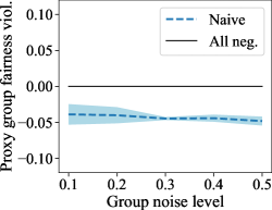

Refer to caption Refer to caption Refer to caption
Figure 4: Maximum fairness constraint violations with respect to the noisy groups G^^𝐺\hat{G} on the test set for different group noise levels γ𝛾\gamma on the Adult dataset. For each noise level, we plot the mean and standard error over 10 random train/val/test splits. The black solid line illustrates a maximum constraint violation of 0. While the naïve approach (left) has increasingly higher fairness constraints with respect to the true groups as the noise increases, it always manages to satisfy the constraints with respect to the noisy groups G^^𝐺\hat{G}

Refer to caption Refer to caption
Figure 5: Maximum robust constraint violations on the test set for different group noise levels P(G^G)𝑃^𝐺𝐺P(\hat{G}\neq G) on the Adult dataset. For each noise level, we plot the mean and standard error over 10 random train/val/test splits. The black dotted line illustrates a maximum constraint violation of 0. Both the DRO approach (left) and the soft group assignments approach (right) managed to satisfy their respective robust constraints on the test set on average for all noise levels.
Table 2: Error rate and fairness constraint violations on the true groups for the Adult dataset (mean and standard error over 10 train/test/splits).
DRO Soft Assignments
Noise Error rate Max G𝐺G Viol. Error rate Max G𝐺G Viol.
0.1 0.152 ±plus-or-minus\pm 0.001 0.002 ±plus-or-minus\pm 0.019 0.148 ±plus-or-minus\pm 0.001 -0.048 ±plus-or-minus\pm 0.002
0.2 0.200 ±plus-or-minus\pm 0.002 -0.045 ±plus-or-minus\pm 0.003 0.157 ±plus-or-minus\pm 0.003 -0.048 ±plus-or-minus\pm 0.002
0.3 0.216 ±plus-or-minus\pm 0.010 -0.044 ±plus-or-minus\pm 0.004 0.158 ±plus-or-minus\pm 0.005 0.002 ±plus-or-minus\pm 0.030
0.4 0.209 ±plus-or-minus\pm 0.006 -0.019 ±plus-or-minus\pm 0.031 0.188 ±plus-or-minus\pm 0.003 -0.016 ±plus-or-minus\pm 0.016
0.5 0.219 ±plus-or-minus\pm 0.012 -0.030 ±plus-or-minus\pm 0.032 0.218 ±plus-or-minus\pm 0.002 0.004 ±plus-or-minus\pm 0.006

F.2.2 Case study 2 (Credit)

This section provides additional experiment results for case study 2 on the Credit dataset.

Figure 6 shows the constraint violations with respect to the true groups on test separated into TPR violations and FPR violations. For all noise levels, there were higher TPR violations than FPR violations. However, this does not mean that the FPR constraint was meaningless – the FPR constraint still ensured that the TPR constraints weren’t satisfied by simply adding false positives.

Figure 7 confirms that the naïve approach, DRO approach, and soft assignments approaches all satisfied the fairness constraints for the noisy groups on the test set.

Figure 8 confirms that the DRO approach and the soft assignments approaches both managed to satisfy their respective robust constraints on the test set on average. For the DRO approach, the constraints measured in Figure 8 come from Equation (3), and for the soft assignments approach, the constraints measured in Figure 8 come from Equation (7).

We provide the exact error rate values and maximum violations on the true groups for the Credit dataset in Table 3.
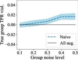
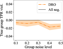
Refer to caption Refer to caption Refer to caption Refer to caption Refer to caption Refer to caption

Figure 6: Case study 2 (Credit): Maximum true group TPR (top) and FPR (bottom) constraint violations for the Naive, DRO, and soft assignments (SA) approaches on test set for different group noise levels γ𝛾\gamma on the Credit dataset (mean and standard error over 10 train/val/test splits). The black solid line represents the performance of the trivial “all negatives” classifier, which has constraint violations of 0. A negative violation indicates satisfaction of the fairness constraints on the true groups.

Refer to caption Refer to caption Refer to caption
Figure 7: Maximum fairness constraint violations with respect to the noisy groups G^^𝐺\hat{G} on the test set for different group noise levels γ𝛾\gamma on the Credit dataset. For each noise level, we plot the mean and standard error over 10 random train/val/test splits. The black solid line illustrates a maximum constraint violation of 0. While the naïve approach (left) has increasingly higher fairness constraints with respect to the true groups as the noise increases, it always manages to satisfy the constraints with respect to the noisy groups G^^𝐺\hat{G}

Refer to caption Refer to caption
Figure 8: Maximum robust constraint violations on the test set for different group noise levels P(G^G)𝑃^𝐺𝐺P(\hat{G}\neq G) on the Credit dataset. For each noise level, we plot the mean and standard error over 10 random train/val/test splits. The black dotted line illustrates a maximum constraint violation of 0. Both the DRO approach (left) and the soft group assignments approach (right) managed to satisfy their respective robust constraints on the test set on average for all noise levels.
Table 3: Error rate and fairness constraint violations on the true groups for the Credit dataset (mean and standard error over 10 train/test/splits).
DRO Soft Assignments
Noise Error rate Max G𝐺G Viol. Error rate Max G𝐺G Viol.
0.1 0.206 ±plus-or-minus\pm 0.003 -0.006 ±plus-or-minus\pm 0.006 0.182 ±plus-or-minus\pm 0.002 0.000 ±plus-or-minus\pm 0.005
0.2 0.209 ±plus-or-minus\pm 0.002 -0.008 ±plus-or-minus\pm 0.008 0.182 ±plus-or-minus\pm 0.001 0.004 ±plus-or-minus\pm 0.005
0.3 0.212 ±plus-or-minus\pm 0.002 -0.006 ±plus-or-minus\pm 0.006 0.198 ±plus-or-minus\pm 0.001 -0.025 ±plus-or-minus\pm 0.007
0.4 0.210 ±plus-or-minus\pm 0.002 -0.017 ±plus-or-minus\pm 0.008 0.213 ±plus-or-minus\pm 0.001 -0.028 ±plus-or-minus\pm 0.005
0.5 0.211 ±plus-or-minus\pm 0.003 -0.015 ±plus-or-minus\pm 0.006 0.211 ±plus-or-minus\pm 0.001 -0.014 ±plus-or-minus\pm 0.004