Online high rank matrix completion

Jicong Fan, Madeleine Udell
Cornell University
Ithaca, NY 14853, USA
{jf577,udell}jf577,udell\left\{\textup{jf577,udell}\right\}@cornell.edu
Abstract

Recent advances in matrix completion enable data imputation in full-rank matrices by exploiting low dimensional (nonlinear) latent structure. In this paper, we develop a new model for high rank matrix completion (HRMC), together with batch and online methods to fit the model and out-of-sample extension to complete new data. The method works by (implicitly) mapping the data into a high dimensional polynomial feature space using the kernel trick; importantly, the data occupies a low dimensional subspace in this feature space, even when the original data matrix is of full-rank. We introduce an explicit parametrization of this low dimensional subspace, and an online fitting procedure, to reduce computational complexity compared to the state of the art. The online method can also handle streaming or sequential data and adapt to non-stationary latent structure. We provide guidance on the sampling rate required these methods to succeed. Experimental results on synthetic data and motion capture data validate the performance of the proposed methods.

1 Introduction

In the past ten years, low rank matrix completion (LRMC) has been widely studied [4, 16, 23, 24, 21, 13, 3, 19, 9]. For instance, Candès and Recht [4] showed that any n×n𝑛𝑛n\times n incoherent matrices of rank r𝑟r can be exactly recovered from Cn1.2rlogn𝐶superscript𝑛1.2𝑟𝑛Cn^{1.2}r\log n uniformly randomly sampled entries with high probability through solving a convex problem of nuclear norm minimization (NNM). However, LRMC cannot recover high rank or full-rank matrices, even when the the data lies on a low dimensional (nonlinear) manifold. To address this problem, recently a few researchers have developed new high rank matrix completion (HRMC) methods [8, 17, 29] for data drawn from multiple subspaces [7, 6, 11] or nonlinear models [1, 25, 10]. These HRMC methods can outperform LRMC methods for many real problems such as subspace clustering with missing data, motion data recovery [6, 25], image inpainting, and classification [1, 10].

All the aforementioned LRMC and HRMC methods are offline methods. However, for many problems, we obtain one sample at a time and would like to update the model as each new sample arrives using online optimization. In addition, compared to offline methods, online methods [26, 22, 30] often have lower space and time complexities and can adapt to changes in the latent data structure. For these reasons, online matrix completion has recently gained increasing attention [2, 5, 15, 20].

2 Related work and our contribution

Online matrix completion.

Sun and Luo [27] and Jin et al. [14] proposed to use stochastic gradient descent (SGD) to solve the low rank factorization (LRF) problem minimize(i,j)Ω(𝑿ij𝑼i:𝑽j:)2minimizesubscript𝑖𝑗Ωsuperscriptsubscript𝑿𝑖𝑗subscript𝑼:𝑖absentsuperscriptsubscript𝑽:𝑗absenttop2\text{minimize}\sum_{(i,j)\in\Omega}\left(\bm{X}_{ij}-\bm{U}_{i:}\bm{V}_{j:}^{\top}\right)^{2} with variables 𝑼m×r𝑼superscript𝑚𝑟\bm{U}\in\mathbb{R}^{m\times r}, 𝑽n×r𝑽superscript𝑛𝑟\bm{V}\in\mathbb{R}^{n\times r}, where 𝑿m×n𝑿superscript𝑚𝑛\bm{X}\in\mathbb{R}^{m\times n}and ΩΩ\Omega denotes the locations of observed entries of 𝑿𝑿\bm{X}. Specifically, given an entry 𝑿ijsubscript𝑿𝑖𝑗\bm{X}_{ij}, the i𝑖i-th row of 𝑼𝑼\bm{U} and j𝑗j-th row of 𝑽𝑽\bm{V} are updated by gradient descent. Yun et al. [30] studied the streaming or online matrix completion problem when the columns of the matrix are presented sequentially. The GROUSE method proposed in [2] used incremental gradient descent on the Grassmannian manifold of subspaces to learn a low rank factorization from incomplete data online. These online methods have a common limitation: they cannot recover high rank matrices. Mairal et al. [22] also studied the online factorization problem with the goal of learning a dictionary for sparse coding: minimize𝑫𝒞,𝜶12𝒙𝑫𝜶2+λ𝜶1𝑫𝒞𝜶minimize12superscriptnorm𝒙𝑫𝜶2𝜆subscriptnorm𝜶1\underset{{\bm{D}\in\mathcal{C},\bm{\alpha}}}{\text{minimize}}\tfrac{1}{2}\|\bm{x}-\bm{D}\bm{\alpha}\|^{2}+\lambda\|\bm{\alpha}\|_{1}. A sparse factorization based matrix completion algorithm was proposed in [11]. It is possible to recover a high rank matrix online by combining ideas from [22] with [11].

High rank matrix completion.

Elhamifar [6] proposed to use group-sparse constraint to complete high rank matrix consisting of data drawn from union of low-dimensional subspaces. Alameda-Pineda et al. [1] proposed a nonlinear matrix completion method for classification. The method performs matrix completion on a matrix consisting of (nonlinear) feature-label pairs, where the unknown labels are regarded as missing entries. The method is inapplicable to general matrix completion problems in which the locations of all missing entries are not necessarily in a single block. Ongie et al. [25] assumed 𝑿𝑿\bm{X} is given by an algebraic variety and proposed a method called VMC to recover the missing entries of 𝑿𝑿\bm{X} through minimizing the rank of ϕ(𝑿)italic-ϕ𝑿\phi(\bm{X}), where ϕ(𝑿)italic-ϕ𝑿\phi(\bm{X}) is a feature matrix given by polynomial kernel. Fan and Chow [10] assumed the data are drawn from a nonlinear latent variable model and proposed a nonlinear matrix completion method (NLMC) that minimizes the rank of ϕ(𝑿)italic-ϕ𝑿\phi(\bm{X}), where ϕ(𝑿)italic-ϕ𝑿\phi(\bm{X}) is composed of high-dimensional nonlinear features induced by polynomial kernel or RBF kernel.

Challenges in HRMC.

First, existing HRMC methods lack strong theoretical guarantee on the sample complexity required for recovery. For example, in VMC, the authors provide a lower bound of sampling rate (ρ0subscript𝜌0\rho_{0}, equation (6) of [25]) only for low-order polynomial kernel and ρ0subscript𝜌0\rho_{0} involved an unknown parameter R𝑅R owing to the algebraic variety assumption. In NLMC [10], the authors only provided a coarse lower bound of sampling rate, i.e. ρ>O(d/m)𝜌𝑂𝑑𝑚\rho>O(d/m), where d𝑑d is the dimension of latent variables. Second, existing HRMC methods are not scalable to large matrices. For example, VMC and NLMC require singular value decomposition on an n×n𝑛𝑛n\times n kernel matrix in every iteration. The method of [6] is also not efficient because of the sparse optimization on an n×n𝑛𝑛n\times n coefficients matrix. Third, existing HRMC methods have no out-of-sample extensions, which means they cannot efficiently complete new data. Last but not least, existing HRMC methods are offline methods and cannot handle online data.

Contributions.

In this paper, we aim to address these challenges. We propose a novel high rank matrix completion method based on kernelized factorization (KFMC). KFMC is more efficient and accurate than state-of-the-art methods. Second, we propose an online version for KFMC, which can outperform online LRMC significantly. Third, we propose an out-of-sample extension for KFMC, which enables us to use the pre-learned high rank model to complete new data directly. Finally, we analyze the sampling rate required for KFMC to succeed.

3 Methodology

3.1 High rank matrices

We assume the columns of 𝑿m×n𝑿superscript𝑚𝑛\bm{X}\in\mathbb{R}^{m\times n} are given by

𝒙=f(𝒔)=[f1(𝒔),f2(𝒔),,fm(𝒔)],𝒙f𝒔superscriptsubscript𝑓1𝒔subscript𝑓2𝒔subscript𝑓𝑚𝒔top\bm{x}=\textbf{f}(\bm{s})=[f_{1}(\bm{s}),f_{2}(\bm{s}),\cdots,f_{m}(\bm{s})]^{\top}, (1)

where 𝒔d𝒔superscript𝑑\bm{s}\in\mathbb{R}^{d} (dm<nmuch-less-than𝑑𝑚𝑛d\ll m<n) consists of uncorrelated variables and each fi:d:subscript𝑓𝑖superscript𝑑f_{i}:\mathbb{R}^{d}\rightarrow\mathbb{R}, i=1,,m𝑖1𝑚i=1,\ldots,m, is a p𝑝p-order polynomial with random coefficients. For example, when d=2𝑑2d=2 and p=2𝑝2p=2, for i=1,,m𝑖1𝑚i=1,\ldots,m, xi=𝒄i𝒔¯subscript𝑥𝑖superscriptsubscript𝒄𝑖top¯𝒔x_{i}=\bm{c}_{i}^{\top}\bar{\bm{s}}, where 𝒄i6subscript𝒄𝑖superscript6\bm{c}_{i}\in\mathbb{R}^{6} and 𝒔¯=[1,s1,s2,s12,s22,s1s2]¯𝒔superscript1subscript𝑠1subscript𝑠2superscriptsubscript𝑠12superscriptsubscript𝑠22subscript𝑠1subscript𝑠2top\bar{\bm{s}}=[1,s_{1},s_{2},s_{1}^{2},s_{2}^{2},s_{1}s_{2}]^{\top}. Lemma 1 shows that 𝑿𝑿\bm{X} is of high rank when p𝑝p is large.

Lemma 1.

Suppose the columns of 𝐗𝐗\bm{X} satisfy (1). Then with probability 1, rank(𝐗)=min{m,n,(d+pp)}rank𝐗𝑚𝑛binomial𝑑𝑝𝑝\textup{rank}(\bm{X})=\min\{m,n,\binom{d+p}{p}\}.

Proof.

Expand the polynomial fisubscript𝑓𝑖f_{i} for each i=1,,m𝑖1𝑚i=1,\ldots,m to write xi=fi(𝒔)=𝒄i𝒔¯subscript𝑥𝑖subscript𝑓𝑖𝒔superscriptsubscript𝒄𝑖top¯𝒔x_{i}=f_{i}(\bm{s})=\bm{c}_{i}^{\top}\bar{\bm{s}}, where 𝒔¯={s1μ1sdμd}|μ|p¯𝒔subscriptsuperscriptsubscript𝑠1subscript𝜇1superscriptsubscript𝑠𝑑subscript𝜇𝑑𝜇𝑝\bar{\bm{s}}=\{s_{1}^{\mu_{1}}\cdots s_{d}^{\mu_{d}}\}_{|\mu|\leq p} and 𝒄i(d+pp)subscript𝒄𝑖superscriptbinomial𝑑𝑝𝑝\bm{c}_{i}\in\mathbb{R}^{\binom{d+p}{p}}. Each column of 𝑿𝑿\bm{X} satisfies 𝒙=𝑪𝒔¯𝒙𝑪¯𝒔\bm{x}=\bm{C}\bar{\bm{s}}, where 𝑪=[𝒄1𝒄m]m×(d+pp)𝑪delimited-[]subscript𝒄1subscript𝒄𝑚superscript𝑚binomial𝑑𝑝𝑝\bm{C}=[\bm{c}_{1}\cdots\bm{c}_{m}]\in\mathbb{R}^{m\times\binom{d+p}{p}}. The matrix 𝑿𝑿\bm{X} can be written as 𝑿=𝑪𝑺¯𝑿𝑪¯𝑺\bm{X}=\bm{C}\bar{\bm{S}}, where 𝑺¯=(𝒔¯1,,𝒔¯n)(d+pp)×n¯𝑺superscriptsubscript¯𝒔1topsuperscriptsubscript¯𝒔𝑛topsuperscriptbinomial𝑑𝑝𝑝𝑛\bar{\bm{S}}=(\bar{\bm{s}}_{1}^{\top},\ldots,\bar{\bm{s}}_{n}^{\top})\in\mathbb{R}^{\binom{d+p}{p}\times n}. The variables 𝒔𝒔\bm{s} are uncorrelated and the coefficients 𝒄𝒄\bm{c} are random, so generically both 𝑪𝑪\bm{C} and 𝑺¯¯𝑺\bar{\bm{S}} are full rank. Hence rank(𝑿)=min{m,n,(d+pp)}rank𝑿𝑚𝑛binomial𝑑𝑝𝑝\textup{rank}(\bm{X})=\min\{m,n,\binom{d+p}{p}\}. ∎

In this paper, our goal is to recover 𝑿𝑿\bm{X} from a few randomly sampled entries we denote by {𝑴ij}(i,j)Ωsubscriptsubscript𝑴𝑖𝑗𝑖𝑗Ω\{\bm{M}_{ij}\}_{(i,j)\in\Omega}. When p𝑝p is large, 𝑿𝑿\bm{X} is generically high rank and cannot be recovered by conventional LRMC methods.

Remark. Throughout this paper, we use the terms “low rank” or “high rank” matrix to mean a matrix whose rank is low or high relative to its side length.

Let ϕ:mm¯:italic-ϕsuperscript𝑚superscript¯𝑚\phi:\mathbb{R}^{m}\rightarrow\mathbb{R}^{\bar{m}} be a q𝑞q-order polynomial feature map ϕ(𝒙)={x1μ1xmμm}|μ|qitalic-ϕ𝒙subscriptsuperscriptsubscript𝑥1subscript𝜇1superscriptsubscript𝑥𝑚subscript𝜇𝑚𝜇𝑞\phi(\bm{x})=\{x_{1}^{\mu_{1}}\cdots x_{m}^{\mu_{m}}\}_{|\mu|\leq q}. Here m¯=(m+qq)¯𝑚binomial𝑚𝑞𝑞{\bar{m}}=\binom{m+q}{q}. Write ϕ(𝑿)=[ϕ(𝒙1),ϕ(𝒙2),,ϕ(𝒙n)]italic-ϕ𝑿italic-ϕsubscript𝒙1italic-ϕsubscript𝒙2italic-ϕsubscript𝒙𝑛\phi(\bm{X})=[\phi(\bm{x}_{1}),\phi(\bm{x}_{2}),\cdots,\phi(\bm{x}_{n})] and consider its rank:

Theorem 1.

Suppose the columns of 𝐗𝐗\bm{X} satisfy (1). Then with probability 1, rank(ϕ(𝐗))=min{m¯,n,(d+pqpq)}rankitalic-ϕ𝐗¯𝑚𝑛binomial𝑑𝑝𝑞𝑝𝑞\textup{rank}(\phi(\bm{X}))=\min\{\bar{m},n,\binom{d+pq}{pq}\}.

Proof.

Define the pq𝑝𝑞pq-order polynomial map ψ(𝒔):=ϕ(𝒙)=ϕ(f(𝒔))assign𝜓𝒔italic-ϕ𝒙italic-ϕf𝒔\psi(\bm{s}):=\phi(\bm{x})=\phi(\textbf{f}(\bm{s})). Expanding as above, write the vector ϕ(𝒙)=𝚿s~italic-ϕ𝒙𝚿~𝑠\phi(\bm{x})=\bm{\Psi}\tilde{s} with 𝚿m¯×(d+pqpq)𝚿superscript¯𝑚binomial𝑑𝑝𝑞𝑝𝑞\bm{\Psi}\in\mathbb{R}^{\bar{m}\times\binom{d+pq}{pq}} and 𝒔~(d+pqpq)~𝒔superscriptbinomial𝑑𝑝𝑞𝑝𝑞\tilde{\bm{s}}\in\mathbb{R}^{\binom{d+pq}{pq}}, and write the matrix ϕ(𝑿)=𝚿𝑺~italic-ϕ𝑿𝚿~𝑺\phi(\bm{X})=\bm{\Psi}\tilde{\bm{S}} with 𝑺~=(𝒔~1,,𝒔~n)(d+pqpq)×n~𝑺superscriptsubscript~𝒔1topsuperscriptsubscript~𝒔𝑛topsuperscriptbinomial𝑑𝑝𝑞𝑝𝑞𝑛\tilde{\bm{S}}=(\tilde{\bm{s}}_{1}^{\top},\ldots,\tilde{\bm{s}}_{n}^{\top})\in\mathbb{R}^{\binom{d+pq}{pq}\times n}. As above, 𝚿𝚿\bm{\Psi} and 𝑺~~𝑺\tilde{\bm{S}} are generically full rank, so rank(ϕ(𝑿))=min{m¯,n,(d+pqpq)}rankitalic-ϕ𝑿¯𝑚𝑛binomial𝑑𝑝𝑞𝑝𝑞\textup{rank}(\phi(\bm{X}))=\min\{\bar{m},n,\binom{d+pq}{pq}\} with probability 1. ∎

While rank(ϕ(𝑿))rank(𝑿)rankitalic-ϕ𝑿rank𝑿\textup{rank}(\phi(\bm{X}))\geq\textup{rank}(\bm{X}), Theorem 1 shows that ϕ(𝑿)italic-ϕ𝑿\phi(\bm{X}) is generically low rank when d𝑑d is small and n𝑛n is large. For example, when d=2𝑑2d=2, m=20𝑚20m=20, n=200𝑛200n=200, p=4𝑝4p=4, and q=2𝑞2q=2, generically rank(𝑿)min{m,n}=0.75rank𝑿𝑚𝑛0.75\tfrac{\text{rank}(\bm{X})}{\min\{m,n\}}=0.75 while rank(ϕ(𝑿))min{m¯,n}=0.225rankitalic-ϕ𝑿¯𝑚𝑛0.225\tfrac{\text{rank}(\phi(\bm{X}))}{\min\{\bar{m},n\}}=0.225: 𝑿𝑿\bm{X} is high rank but ϕ(𝑿)italic-ϕ𝑿\phi(\bm{X}) is low rank.

3.2 Kernelized factorization

To recover the missing entries of 𝑿𝑿\bm{X}, we propose to solve

minimize𝑿,𝑨,𝒁12ϕ(𝑿)𝑨𝒁F2subject to𝑿ij=𝑴ij,(i,j)Ω,subscriptminimize𝑿𝑨𝒁12superscriptsubscriptnormitalic-ϕ𝑿𝑨𝒁𝐹2subject toformulae-sequencesubscript𝑿𝑖𝑗subscript𝑴𝑖𝑗𝑖𝑗Ω\begin{array}[]{ll}\mathop{\text{minimize}}_{\bm{X},\bm{A},\bm{Z}}&\tfrac{1}{2}\|\phi(\bm{X})-\bm{A}\bm{Z}\|_{F}^{2}\\ \mbox{subject to}&\bm{X}_{ij}=\bm{M}_{ij},\ (i,j)\in\Omega,\end{array} (2)

where 𝑨m¯×r𝑨superscript¯𝑚𝑟\bm{A}\in\mathbb{R}^{\bar{m}\times r}, 𝒁r×n𝒁superscript𝑟𝑛\bm{Z}\in\mathbb{R}^{r\times n}, and r=(d+pqpq)𝑟binomial𝑑𝑝𝑞𝑝𝑞r=\binom{d+pq}{pq}. The solution to (2) completes the entries of 𝑿𝑿\bm{X} using the natural low rank structure of ϕ(𝑿)italic-ϕ𝑿\phi(\bm{X}). Problem (2) implicitly defines an estimate for f𝑓f, f^(𝑺):=𝑿ϕ1(𝑨𝒁)assign^f𝑺𝑿superscriptitalic-ϕ1𝑨𝒁\hat{\textbf{f}}(\bm{S}):=\bm{X}\approx\phi^{-1}(\bm{A}\bm{Z}).

For numerical stability, we regularize 𝑨𝑨\bm{A} and 𝒁𝒁\bm{Z} and solve

minimize𝑿,𝑨,𝒁subscriptminimize𝑿𝑨𝒁\displaystyle\mathop{\text{minimize}}_{\bm{X},\bm{A},\bm{Z}} 12ϕ(𝑿)𝑨𝒁F2+α2𝑨F2+β2𝒁F2,12superscriptsubscriptnormitalic-ϕ𝑿𝑨𝒁𝐹2𝛼2superscriptsubscriptnorm𝑨𝐹2𝛽2superscriptsubscriptnorm𝒁𝐹2\displaystyle\tfrac{1}{2}\|\phi(\bm{X})-\bm{A}\bm{Z}\|_{F}^{2}+\tfrac{\alpha}{2}\|\bm{A}\|_{F}^{2}+\tfrac{\beta}{2}\|\bm{Z}\|_{F}^{2}, (3)
subject to 𝑿ij=𝑴ij,(i,j)Ω,formulae-sequencesubscript𝑿𝑖𝑗subscript𝑴𝑖𝑗𝑖𝑗Ω\displaystyle\bm{X}_{ij}=\bm{M}_{ij},\ (i,j)\in\Omega,

where α𝛼\alpha and β𝛽\beta are regularization parameters, instead of (2).

It is possible to solve (3) directly but the computational cost is quite high if m𝑚m and q𝑞q are large. The following lemma shows that there is no need to model 𝑨𝑨\bm{A} explicitly.

Lemma 2.

For any 𝐗𝐗\bm{X} generated by (1), there exist 𝐃m×r𝐃superscript𝑚𝑟\bm{D}\in\mathbb{R}^{m\times r} and 𝐙r×n𝐙superscript𝑟𝑛\bm{Z}\in\mathbb{R}^{r\times n} such that ϕ(𝐗)=ϕ(𝐃)𝐙italic-ϕ𝐗italic-ϕ𝐃𝐙\phi(\bm{X})=\phi(\bm{D})\bm{Z}.

Proof.

Suppose 𝑫m×r𝑫superscript𝑚𝑟\bm{D}\in\mathbb{R}^{m\times r} are also generated by (1) (e.g. any r𝑟r columns of 𝑿𝑿\bm{X}), so ϕ(𝑫)italic-ϕ𝑫\phi(\bm{D}) and ϕ(𝑿)italic-ϕ𝑿\phi(\bm{X}) share their column space and (with probability 1) ϕ(𝑫)italic-ϕ𝑫\phi(\bm{D}) is full rank. More precisely, ϕ(𝑫)=𝑩𝑪𝑫italic-ϕ𝑫𝑩subscript𝑪𝑫\phi(\bm{D})=\bm{B}\bm{C}_{\scalebox{0.6}{$\bm{D}$}} and ϕ(𝑿)=𝑩𝑪𝑿italic-ϕ𝑿𝑩subscript𝑪𝑿\phi(\bm{X})=\bm{B}\bm{C}_{\scalebox{0.6}{$\bm{X}$}}, where 𝑩m¯×r𝑩superscript¯𝑚𝑟\bm{B}\in\mathbb{R}^{\bar{m}\times r} is a basis for the column space, and both 𝑪𝑿r×nsubscript𝑪𝑿superscript𝑟𝑛\bm{C}_{\scalebox{0.6}{$\bm{X}$}}\in\mathbb{R}^{r\times n} and 𝑪𝑫r×rsubscript𝑪𝑫superscript𝑟𝑟\bm{C}_{\scalebox{0.6}{$\bm{D}$}}\in\mathbb{R}^{r\times r} are full rank. Define 𝒁=𝑪𝑫1𝑪𝑿𝒁superscriptsubscript𝑪𝑫1subscript𝑪𝑿\bm{Z}=\bm{C}_{\scalebox{0.6}{$\bm{D}$}}^{-1}\bm{C}_{\scalebox{0.6}{$\bm{X}$}} and the result follows. ∎

Hence any solution of the following also solves (3):

minimize𝑿,𝑫,𝒁subscriptminimize𝑿𝑫𝒁\displaystyle\mathop{\text{minimize}}_{\bm{X},\bm{D},\bm{Z}}\ 12ϕ(𝑿)ϕ(𝑫)𝒁F2+α2ϕ(𝑫)F2+β2𝒁F212superscriptsubscriptnormitalic-ϕ𝑿italic-ϕ𝑫𝒁𝐹2𝛼2superscriptsubscriptnormitalic-ϕ𝑫𝐹2𝛽2superscriptsubscriptnorm𝒁𝐹2\displaystyle\tfrac{1}{2}\|\phi(\bm{X})-\phi(\bm{D})\bm{Z}\|_{F}^{2}+\tfrac{\alpha}{2}\|\phi(\bm{D})\|_{F}^{2}+\tfrac{\beta}{2}\|\bm{Z}\|_{F}^{2}
subject to 𝑿ij=𝑴ij,(i,j)Ω,formulae-sequencesubscript𝑿𝑖𝑗subscript𝑴𝑖𝑗𝑖𝑗Ω\displaystyle\bm{X}_{ij}=\bm{M}_{ij},\ (i,j)\in\Omega, (4)

where 𝑫m×r𝑫superscript𝑚𝑟\bm{D}\in\mathbb{R}^{m\times r} is much smaller than 𝑨m¯×r𝑨superscript¯𝑚𝑟\bm{A}\in\mathbb{R}^{\bar{m}\times r} of (3). Use the trace function Tr to rewrite the objective in (4) as

12Tr(ϕ(𝑿)ϕ(𝑿)2ϕ(𝑿)ϕ(𝑫)𝒁+𝒁ϕ(𝑫)ϕ(𝑫)𝒁)12Tritalic-ϕsuperscript𝑿topitalic-ϕ𝑿2italic-ϕsuperscript𝑿topitalic-ϕ𝑫𝒁superscript𝒁topitalic-ϕsuperscript𝑫topitalic-ϕ𝑫𝒁\displaystyle\tfrac{1}{2}\text{Tr}\left(\phi(\bm{X})^{\top}\phi(\bm{X})-2\phi(\bm{X})^{\top}\phi(\bm{D})\bm{Z}+\bm{Z}^{\top}\phi(\bm{D})^{\top}\phi(\bm{D})\bm{Z}\right)
+α2Tr(ϕ(𝑫)ϕ(𝑫))+β2𝒁F2.𝛼2Tritalic-ϕsuperscript𝑫topitalic-ϕ𝑫𝛽2superscriptsubscriptnorm𝒁𝐹2\displaystyle+\tfrac{\alpha}{2}\text{Tr}\left(\phi(\bm{D})^{\top}\phi(\bm{D})\right)+\tfrac{\beta}{2}\|\bm{Z}\|_{F}^{2}.

Now we use the kernel trick to avoid explicitly computing the feature map ϕitalic-ϕ\phi. Define k(𝒙,𝒚):=ϕ(𝒙)ϕ(𝒚)=ϕ(𝒙),ϕ(𝒚)assign𝑘𝒙𝒚italic-ϕsuperscript𝒙topitalic-ϕ𝒚italic-ϕ𝒙italic-ϕ𝒚k(\bm{x},\bm{y}):=\phi(\bm{x})^{\top}\phi(\bm{y})=\langle\phi(\bm{x}),\phi(\bm{y})\rangle, so ϕ(𝑿)ϕ(𝑿)=𝑲𝑿𝑿italic-ϕsuperscript𝑿topitalic-ϕ𝑿subscript𝑲𝑿𝑿\phi(\bm{X})^{\top}\phi(\bm{X})=\bm{K}_{\scalebox{0.6}{$\bm{X}\bm{X}$}}, ϕ(𝑿)ϕ(𝑫)=𝑲𝑿𝑫italic-ϕsuperscript𝑿topitalic-ϕ𝑫subscript𝑲𝑿𝑫\phi(\bm{X})^{\top}\phi(\bm{D})=\bm{K}_{\scalebox{0.6}{$\bm{X}\bm{D}$}}, and ϕ(𝑫)ϕ(𝑫)=𝑲𝑫𝑫italic-ϕsuperscript𝑫topitalic-ϕ𝑫subscript𝑲𝑫𝑫\phi(\bm{D})^{\top}\phi(\bm{D})=\bm{K}_{\scalebox{0.6}{$\bm{D}\bm{D}$}}, where 𝑲𝑿𝑿subscript𝑲𝑿𝑿\bm{K}_{\scalebox{0.6}{$\bm{X}\bm{X}$}}, 𝑲𝑿𝑫subscript𝑲𝑿𝑫\bm{K}_{\scalebox{0.6}{$\bm{X}\bm{D}$}}, and 𝑲𝑫𝑫subscript𝑲𝑫𝑫\bm{K}_{\scalebox{0.6}{$\bm{D}\bm{D}$}} are the corresponding kernel matrices. The most widely-used kernels are the polynomial kernel (Poly) and the radial basis function kernel (RBF)

Poly:k(𝒙,𝒚)=(𝒙𝒚+c)q:Poly𝑘𝒙𝒚superscriptsuperscript𝒙top𝒚𝑐𝑞\displaystyle\mbox{Poly}:\ k(\bm{x},\bm{y})=(\bm{x}^{\top}\bm{y}+c)^{q} (5)
RBF:k(𝒙,𝒚)=exp(1σ2𝒙𝒚2),:RBF𝑘𝒙𝒚1superscript𝜎2superscriptnorm𝒙𝒚2\displaystyle\mbox{RBF}:\ k(\bm{x},\bm{y})=\exp\left(-\tfrac{1}{\sigma^{2}}\|\bm{x}-\bm{y}\|^{2}\right),

with hyperparameters c𝑐c, q𝑞q, and σ𝜎\sigma. The (implicit) feature maps ϕ(𝒙)italic-ϕ𝒙\phi(\bm{x}) of Poly and RBF are the q𝑞q-order and infinite-order polynomial maps respectively. Rewrite (4) to define kernelized factorizatiom matrix completion (KFMC)

minimize𝑿,𝑫,𝒁subscriptminimize𝑿𝑫𝒁\displaystyle\mathop{\text{minimize}}_{\bm{X},\bm{D},\bm{Z}} (𝒁,𝑫,𝑿)𝒁𝑫𝑿\displaystyle\ell(\bm{Z},\bm{D},\bm{X}) (KFMC)
subject to 𝑿ij=𝑴ij,(i,j)Ωformulae-sequencesubscript𝑿𝑖𝑗subscript𝑴𝑖𝑗𝑖𝑗Ω\displaystyle\bm{X}_{ij}=\bm{M}_{ij},\ (i,j)\in\Omega

where (𝒁,𝑫,𝑿)=12Tr(𝑲𝑿𝑿2𝑲𝑿𝑫𝒁+𝒁𝑲𝑫𝑫𝒁)+α2Tr(𝑲𝑫𝑫)+β2𝒁F2.𝒁𝑫𝑿12Trsubscript𝑲𝑿𝑿2subscript𝑲𝑿𝑫𝒁superscript𝒁topsubscript𝑲𝑫𝑫𝒁𝛼2Trsubscript𝑲𝑫𝑫𝛽2superscriptsubscriptnorm𝒁𝐹2\ell(\bm{Z},\bm{D},\bm{X})=\tfrac{1}{2}\text{Tr}\left(\bm{K}_{\scalebox{0.6}{$\bm{X}\bm{X}$}}-2\bm{K}_{\scalebox{0.6}{$\bm{X}\bm{D}$}}\bm{Z}+\bm{Z}^{\top}\bm{K}_{\scalebox{0.6}{$\bm{D}\bm{D}$}}\bm{Z}\right)+\tfrac{\alpha}{2}\text{Tr}(\bm{K}_{\scalebox{0.6}{$\bm{D}\bm{D}$}})+\tfrac{\beta}{2}\|\bm{Z}\|_{F}^{2}. For the RBF kernel, Tr(𝑲𝑫𝑫)rTrsubscript𝑲𝑫𝑫𝑟\text{Tr}(\bm{K}_{\scalebox{0.6}{$\bm{D}\bm{D}$}})\equiv r is a constant and can be dropped from the objective.

3.3 Optimization for KFMC

The optimization problem (KFMC) is nonconvex and has three blocks of variables. We propose using coordinate descent over these three blocks to find a stationary point.

Update 𝒁𝒁\bm{Z}.

To begin, complete entries of 𝑿𝑿\bm{X} arbitrarily and randomly initialize 𝑫𝑫\bm{D}. Define the r×r𝑟𝑟r\times r identity 𝑰rsubscript𝑰𝑟\bm{I}_{r}. Fix 𝑿𝑿\bm{X} and 𝑫𝑫\bm{D} and update 𝒁𝒁\bm{Z} as

𝒁𝒁\displaystyle\bm{Z} arg min𝒁(𝒁,𝑫,𝑿)absentsubscriptarg min𝒁𝒁𝑫𝑿\displaystyle\leftarrow\mathop{\text{arg min}}_{\bm{Z}}\ell(\bm{Z},\bm{D},\bm{X})
=arg min𝒁Tr(𝑲𝑿𝑫𝒁)+12Tr(𝒁𝑲𝑫𝑫𝒁)+β2𝒁F2absentsubscriptarg min𝒁Trsubscript𝑲𝑿𝑫𝒁12Trsuperscript𝒁topsubscript𝑲𝑫𝑫𝒁𝛽2superscriptsubscriptnorm𝒁𝐹2\displaystyle=\mathop{\text{arg min}}_{\bm{Z}}-\text{Tr}(\bm{K}_{\scalebox{0.6}{$\bm{X}\bm{D}$}}\bm{Z})+\tfrac{1}{2}\text{Tr}(\bm{Z}^{\top}\bm{K}_{\scalebox{0.6}{$\bm{D}\bm{D}$}}\bm{Z})+\tfrac{\beta}{2}\|\bm{Z}\|_{F}^{2}
=(𝑲𝑫𝑫+β𝑰r)1𝑲𝑿𝑫,absentsuperscriptsubscript𝑲𝑫𝑫𝛽subscript𝑰𝑟1superscriptsubscript𝑲𝑿𝑫top\displaystyle=(\bm{K}_{\scalebox{0.6}{$\bm{D}\bm{D}$}}+\beta\bm{I}_{r})^{-1}\bm{K}_{\scalebox{0.6}{$\bm{X}\bm{D}$}}^{\top}, (6)

Update 𝑫𝑫\bm{D}.

There is no closed form solution for the minimization of (𝒁,𝑫,𝑿)𝒁𝑫𝑿\ell(\bm{Z},\bm{D},\bm{X}) with respect to 𝑫𝑫\bm{D} due to the kernel matrices. Instead, we propose the additive update 𝑫𝑫𝚫𝑫𝑫𝑫subscript𝚫𝑫\bm{D}\leftarrow\bm{D}-\bm{\Delta}_{\scalebox{0.6}{$\bm{D}$}}. We compute 𝚫𝑫subscript𝚫𝑫\bm{\Delta}_{\scalebox{0.6}{$\bm{D}$}} using a relaxed Newton method, described below for the Poly and RBF kernels.

For the polynomial kernel, rewrite the terms in the objective in which 𝑫𝑫\bm{D} appears as

(𝒁,𝑫,𝑿):=Tr((𝑾1(𝑿T𝑫+c))𝒁)+12Tr(𝒁T(𝑾2(𝑫T𝑫+c))𝒁)+α2Tr(𝑾2(𝑫T𝑫+c)).assign𝒁𝑫𝑿absentTrdirect-productsubscript𝑾1superscript𝑿𝑇𝑫𝑐𝒁missing-subexpression12Trsuperscript𝒁𝑇direct-productsubscript𝑾2superscript𝑫𝑇𝑫𝑐𝒁missing-subexpression𝛼2Trdirect-productsubscript𝑾2superscript𝑫𝑇𝑫𝑐\displaystyle\begin{aligned} \ell(\bm{Z},\bm{D},\bm{X}):=&-\text{Tr}((\bm{W}_{1}\odot(\bm{X}^{T}\bm{D}+c))\bm{Z})\\ &+\tfrac{1}{2}\text{Tr}(\bm{Z}^{T}(\bm{W}_{2}\odot(\bm{D}^{T}\bm{D}+c))\bm{Z})\\ &+\tfrac{\alpha}{2}\text{Tr}(\bm{W}_{2}\odot(\bm{D}^{T}\bm{D}+c)).\end{aligned} (7)

defining 𝑾1=𝑿𝑫+cq1subscript𝑾1superscriptdelimited-⟨⟩superscript𝑿top𝑫𝑐𝑞1\bm{W}_{1}=\langle\bm{X}^{\top}\bm{D}+c\rangle^{q-1} and 𝑾2=𝑫𝑫+cq1subscript𝑾2superscriptdelimited-⟨⟩superscript𝑫top𝑫𝑐𝑞1\bm{W}_{2}=\langle\bm{D}^{\top}\bm{D}+c\rangle^{q-1}, where direct-product\odot is elementwise multiplication and usuperscriptdelimited-⟨⟩𝑢\langle\cdot\rangle^{u} denotes the element-wise u𝑢u-power. Inspired by iteratively reweighted optimization, fix 𝑾1subscript𝑾1\bm{W}_{1} and 𝑾2subscript𝑾2\bm{W}_{2} to approximate the gradient and Hessian of (𝒁,𝑫,𝑿)𝒁𝑫𝑿\ell(\bm{Z},\bm{D},\bm{X}) with respect to 𝑫𝑫\bm{D} as

𝒈𝑫subscript𝒈𝑫\displaystyle\bm{g}_{\scalebox{0.6}{$\bm{D}$}} :=𝑿(𝑾1𝒁)+𝑫((𝒁𝒁+α𝑰r𝑾2))assignabsent𝑿direct-productsubscript𝑾1superscript𝒁top𝑫𝒁superscript𝒁topdirect-product𝛼subscript𝑰𝑟subscript𝑾2\displaystyle:=-\bm{X}(\bm{W}_{1}\odot\bm{Z}^{\top})+\bm{D}((\bm{Z}\bm{Z}^{\top}+\alpha\bm{I}_{r}\odot\bm{W}_{2}))
𝑯𝑫subscript𝑯𝑫\displaystyle\bm{H}_{\scalebox{0.6}{$\bm{D}$}} :=𝒁𝒁𝑾2+α𝑾2𝑰r.assignabsentdirect-product𝒁superscript𝒁topsubscript𝑾2direct-product𝛼subscript𝑾2subscript𝑰𝑟\displaystyle:=\bm{Z}\bm{Z}^{\top}\odot\bm{W}_{2}+\alpha\bm{W}_{2}\odot\bm{I}_{r}.

𝑯𝑫subscript𝑯𝑫\bm{H}_{\scalebox{0.6}{$\bm{D}$}} is positive definite by the Schur product theorem. Now choose τ>1𝜏1\tau>1 for numerical stability and define the update

𝚫𝑫:=1τ𝒈𝑫𝑯𝑫1.assignsubscript𝚫𝑫1𝜏subscript𝒈𝑫superscriptsubscript𝑯𝑫1\bm{\Delta}_{\scalebox{0.6}{$\bm{D}$}}:=\tfrac{1}{\tau}\bm{g}_{\scalebox{0.6}{$\bm{D}$}}\bm{H}_{\scalebox{0.6}{$\bm{D}$}}^{-1}. (8)

The effectiveness of our update for 𝑫𝑫\bm{D} is guaranteed by the following lemma. (The proof of the lemma and discussion about the role of τ𝜏\tau are in the supplementary material.)

Lemma 3.

The update (8) is a relaxed Newton’s method and ensures sufficient decrease in the objective:

(𝒁,𝑫𝚫𝑫,𝑿)(𝒁,𝑫,𝑿)12τTr(𝒈𝑫𝑯𝑫1𝒈𝑫).𝒁𝑫subscript𝚫𝑫𝑿𝒁𝑫𝑿12𝜏Trsubscript𝒈𝑫superscriptsubscript𝑯𝑫1superscriptsubscript𝒈𝑫top\ell(\bm{Z},\bm{D}-\bm{\Delta}_{\scalebox{0.6}{$\bm{D}$}},\bm{X})-\ell(\bm{Z},\bm{D},\bm{X})\leq-\tfrac{1}{2\tau}\textup{Tr}(\bm{g}_{\scalebox{0.6}{$\bm{D}$}}\bm{H}_{\scalebox{0.6}{$\bm{D}$}}^{-1}\bm{g}_{\scalebox{0.6}{$\bm{D}$}}^{\top}).

For the RBF kernel, the gradient is

𝑫=1σ2(𝑿𝑸1𝑫𝚪1)+2σ2(𝑫𝑸2𝑫𝚪2).subscript𝑫1superscript𝜎2𝑿subscript𝑸1𝑫subscript𝚪12superscript𝜎2𝑫subscript𝑸2𝑫subscript𝚪2\nabla_{\scalebox{0.6}{$\bm{D}$}}\ell=\tfrac{1}{\sigma^{2}}(\bm{X}\bm{Q}_{1}-\bm{D}\bm{\Gamma}_{1})+\tfrac{2}{\sigma^{2}}(\bm{D}\bm{Q}_{2}-\bm{D}\bm{\Gamma}_{2}). (9)

(Throughout, we abuse notation to write \ell for (𝒁,𝑫,𝑿)𝒁𝑫𝑿\ell(\bm{Z},\bm{D},\bm{X}).) Here 𝑸1=𝒁𝑲𝑿𝑫subscript𝑸1direct-productsuperscript𝒁topsubscript𝑲𝑿𝑫\bm{Q}_{1}=-\bm{Z}^{\top}\odot\bm{K}_{\scalebox{0.6}{$\bm{X}\bm{D}$}}, 𝑸2=(0.5𝒁𝒁+0.5α𝑰r)𝑲𝑫𝑫subscript𝑸2direct-product0.5𝒁superscript𝒁top0.5𝛼subscript𝑰𝑟subscript𝑲𝑫𝑫\bm{Q}_{2}=(0.5\bm{Z}\bm{Z}^{\top}+0.5\alpha\bm{I}_{r})\odot\bm{K}_{\scalebox{0.6}{$\bm{D}\bm{D}$}}, 𝚪1=diag(𝟏n𝑸1)subscript𝚪1diagsuperscriptsubscript1𝑛topsubscript𝑸1\bm{\Gamma}_{1}=\mbox{diag}(\bm{1}_{n}^{\top}\bm{Q}_{1}), and 𝚪2=diag(𝟏r𝑸2)subscript𝚪2diagsuperscriptsubscript1𝑟topsubscript𝑸2\bm{\Gamma}_{2}=\mbox{diag}(\bm{1}_{r}^{\top}\bm{Q}_{2}), where 𝟏nnsubscript1𝑛superscript𝑛\bm{1}_{n}\in\mathbb{R}^{n} and 𝟏rrsubscript1𝑟superscript𝑟\bm{1}_{r}\in\mathbb{R}^{r} are composed of 1s. The following lemma (proved in the supplementary material) indicates that 𝑿𝑸1𝑿subscript𝑸1\bm{X}\bm{Q}_{1} in (9) is nearly a constant compared to 𝑫𝚪1𝑫subscript𝚪1\bm{D}\bm{\Gamma}_{1}, 𝑫𝑸2𝑫subscript𝑸2\bm{D}\bm{Q}_{2}, and 𝑫𝚪2𝑫subscript𝚪2\bm{D}\bm{\Gamma}_{2}, provided that σ𝜎\sigma and n𝑛n are large enough:

Lemma 4.

𝑿(𝒁𝑲𝑿𝑫1)𝑿(𝒁𝑲𝑿𝑫2)Fcσn𝑿2𝑫1𝑫2Fsubscriptnorm𝑿direct-productsuperscript𝒁topsubscript𝑲𝑿subscript𝑫1𝑿direct-productsuperscript𝒁topsubscript𝑲𝑿subscript𝑫2𝐹𝑐𝜎𝑛subscriptnorm𝑿2subscriptnormsubscript𝑫1subscript𝑫2𝐹\|\bm{X}(\bm{Z}^{\top}\odot\bm{K}_{\scalebox{0.6}{$\bm{X}\bm{D}_{1}$}})-\bm{X}(\bm{Z}^{\top}\odot\bm{K}_{\scalebox{0.6}{$\bm{X}\bm{D}_{2}$}})\|_{F}\leq\tfrac{c}{\sigma\sqrt{n}}\|\bm{X}\|_{2}\|\bm{D}_{1}-\bm{D}_{2}\|_{F}, where c𝑐c is a small constant.

Therefore, we can compute an approximate Hessian neglecting 𝑿𝑸1𝑿subscript𝑸1\bm{X}\bm{Q}_{1}. As in (8), we define

𝚫𝑫:=1τ𝑫(1σ2(2𝑸2𝚪12𝚪2))1.assignsubscript𝚫𝑫1𝜏subscript𝑫superscript1superscript𝜎22subscript𝑸2subscript𝚪12subscript𝚪21\bm{\Delta}_{\scalebox{0.6}{$\bm{D}$}}:=\tfrac{1}{\tau}\nabla_{\scalebox{0.6}{$\bm{D}$}}\ell(\tfrac{1}{\sigma^{2}}(2\bm{Q}_{2}-\bm{\Gamma}_{1}-2\bm{\Gamma}_{2}))^{-1}. (10)

Update 𝑿𝑿\bm{X}.

Finally, fixing 𝒁𝒁\bm{Z} and 𝑫𝑫\bm{D}, we wish to minimize (KFMC) over 𝑿𝑿\bm{X}, which again has no closed-form solution. Again, we suggest updating 𝑿𝑿\bm{X} using a relaxed Newton method 𝑿𝑿𝚫𝑿𝑿𝑿subscript𝚫𝑿\bm{X}\leftarrow\bm{X}-\bm{\Delta}_{\scalebox{0.6}{$\bm{X}$}}. For the polynomial kernel,

𝒈𝑿subscript𝒈𝑿\displaystyle\bm{g}_{\scalebox{0.6}{$\bm{X}$}} =𝑿(𝑾3𝑰n)𝑫(𝑾4𝒁)absent𝑿direct-productsubscript𝑾3subscript𝑰𝑛𝑫direct-productsuperscriptsubscript𝑾4top𝒁\displaystyle=\bm{X}(\bm{W}_{3}\odot\bm{I}_{n})-\bm{D}(\bm{W}_{4}^{\top}\odot\bm{Z}) (11)
=q𝑿(𝟏m𝒘)q𝑫(𝑾4𝒁),absentdirect-product𝑞𝑿subscript1𝑚superscript𝒘top𝑞𝑫direct-productsuperscriptsubscript𝑾4top𝒁\displaystyle=q\bm{X}\odot(\bm{1}_{m}\bm{w}^{\top})-q\bm{D}(\bm{W}_{4}^{\top}\odot\bm{Z}),

where 𝑾3=𝑿𝑿+cq1subscript𝑾3superscriptdelimited-⟨⟩superscript𝑿top𝑿𝑐𝑞1\bm{W}_{3}=\langle\bm{X}^{\top}\bm{X}+c\rangle^{q-1}, 𝑾4=𝑿𝑫+cq1subscript𝑾4superscriptdelimited-⟨⟩superscript𝑿top𝑫𝑐𝑞1\bm{W}_{4}=\langle\bm{X}^{\top}\bm{D}+c\rangle^{q-1}, 𝟏mmsubscript1𝑚superscript𝑚\bm{1}_{m}\in\mathbb{R}^{m} consists of 1s, and 𝒘m𝒘superscript𝑚\bm{w}\in\mathbb{R}^{m} consists of the diagonal entries of 𝑾3subscript𝑾3\bm{W}_{3}. As above, we define

𝚫𝑿:=1τ𝒈𝑿(𝟏m𝒘T).assignsubscript𝚫𝑿direct-product1𝜏subscript𝒈𝑿subscript1𝑚superscript𝒘𝑇\bm{\Delta}_{\scalebox{0.6}{$\bm{X}$}}:=\tfrac{1}{\tau}\bm{g}_{\scalebox{0.6}{$\bm{X}$}}\odot(\bm{1}_{m}\bm{w}^{-T}). (12)

When RBF kernel is used, we get

𝑿=1σ2(𝑫𝑸3𝑿𝚪3)+2σ2(𝑿𝑸4𝑿𝚪4).subscript𝑿1superscript𝜎2𝑫subscript𝑸3𝑿subscript𝚪32superscript𝜎2𝑿subscript𝑸4𝑿subscript𝚪4\nabla_{\scalebox{0.6}{$\bm{X}$}}\ell=\tfrac{1}{\sigma^{2}}(\bm{D}\bm{Q}_{3}-\bm{X}\bm{\Gamma}_{3})+\tfrac{2}{\sigma^{2}}(\bm{X}\bm{Q}_{4}-\bm{X}\bm{\Gamma}_{4}). (13)

Here 𝑸3=𝒁𝑲𝑿𝑫subscript𝑸3direct-product𝒁superscriptsubscript𝑲𝑿𝑫top\bm{Q}_{3}=-\bm{Z}\odot\bm{K}_{\scalebox{0.6}{$\bm{X}\bm{D}$}}^{\top}, 𝑸4=0.5𝑰n𝑲𝑿𝑿subscript𝑸4direct-product0.5subscript𝑰𝑛subscript𝑲𝑿𝑿\bm{Q}_{4}=0.5\bm{I}_{n}\odot\bm{K}_{\scalebox{0.6}{$\bm{X}\bm{X}$}}, 𝚪3=diag(𝟏r𝑸3)subscript𝚪3diagsuperscriptsubscript1𝑟topsubscript𝑸3\bm{\Gamma}_{3}=\mbox{diag}(\bm{1}_{r}^{\top}\bm{Q}_{3}), and 𝚪4=diag(𝟏n𝑸4)subscript𝚪4diagsuperscriptsubscript1𝑛topsubscript𝑸4\bm{\Gamma}_{4}=\mbox{diag}(\bm{1}_{n}^{\top}\bm{Q}_{4}). As in (10), define

𝚫𝑿:=1τ𝑿(1σ2(2𝑸4𝚪32𝚪4))1.assignsubscript𝚫𝑿1𝜏subscript𝑿superscript1superscript𝜎22subscript𝑸4subscript𝚪32subscript𝚪41\bm{\Delta}_{\scalebox{0.6}{$\bm{X}$}}:=\tfrac{1}{\tau}\nabla_{\scalebox{0.6}{$\bm{X}$}}\ell(\tfrac{1}{\sigma^{2}}(2\bm{Q}_{4}-\bm{\Gamma}_{3}-2\bm{\Gamma}_{4}))^{-1}. (14)

Here the computational cost is not high in practice because the matrix to be inverted is diagonal.

We can also use a momentum update to accelerate the convergence of 𝑫𝑫\bm{D} and 𝑿𝑿\bm{X}:

{𝚫^𝑫η𝚫^𝑫+𝚫𝑫,𝑫𝑫𝚫^𝑫𝚫^𝑿η𝚫^𝑿+𝚫𝑿,𝑿𝑿𝚫^𝑿\left\{\begin{aligned} &\widehat{\bm{\Delta}}_{\scalebox{0.6}{$\bm{D}$}}\leftarrow\eta\widehat{\bm{\Delta}}_{\scalebox{0.6}{$\bm{D}$}}+\bm{\Delta}_{\scalebox{0.6}{$\bm{D}$}},\ \bm{D}\leftarrow\bm{D}-\widehat{\bm{\Delta}}_{\scalebox{0.6}{$\bm{D}$}}\\ &\widehat{\bm{\Delta}}_{\scalebox{0.6}{$\bm{X}$}}\leftarrow\eta\widehat{\bm{\Delta}}_{\scalebox{0.6}{$\bm{X}$}}+\bm{\Delta}_{\scalebox{0.6}{$\bm{X}$}},\ \bm{X}\leftarrow\bm{X}-\widehat{\bm{\Delta}}_{\scalebox{0.6}{$\bm{X}$}}\\ \end{aligned}\right. (15)

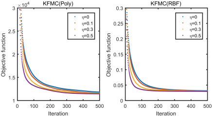
where 0<η<10𝜂10<\eta<1 is a constant. The optimization method is summarized as Algorithm 1. The following lemma (with proof in the supplement) shows the method converges.

Lemma 5.

For sufficiently small η𝜂\eta, Algorithm 1 converges to a stationary point.

Algorithm 1 Offline KFMC
1:𝑴𝑴\bm{M}, ΩΩ\Omega, r𝑟r, k(,)𝑘k(\cdot,\cdot), α𝛼\alpha, β𝛽\beta, tmaxsubscript𝑡maxt_{\text{max}}, η𝜂\eta
2:Initialize: t=0𝑡0t=0, 𝑿𝑿\bm{X}, 𝑫𝒩(0,1)similar-to𝑫𝒩01\bm{D}\sim\mathcal{N}(0,1), 𝚫^𝑫=𝟎subscript^𝚫𝑫0\widehat{\bm{\Delta}}_{\scalebox{0.6}{$\bm{D}$}}=\bm{0}, 𝚫^𝑿=𝟎subscript^𝚫𝑿0\widehat{\bm{\Delta}}_{\scalebox{0.6}{$\bm{X}$}}=\bm{0}
3:repeat
4:     tt+1𝑡𝑡1t\leftarrow t+1
5:     𝒁=(𝑲𝑫𝑫+β𝑰r)1𝑲𝑿𝑫𝒁superscriptsubscript𝑲𝑫𝑫𝛽subscript𝑰𝑟1superscriptsubscript𝑲𝑿𝑫top\bm{Z}=(\bm{K}_{\scalebox{0.6}{$\bm{D}\bm{D}$}}+\beta\bm{I}_{r})^{-1}\bm{K}_{\scalebox{0.6}{$\bm{X}\bm{D}$}}^{\top}
6:     Compute 𝚫𝑫subscript𝚫𝑫\bm{\Delta}_{\scalebox{0.6}{$\bm{D}$}} using (8) or (10)
7:     𝚫^𝑫=η𝚫^𝑫+𝚫𝑫subscript^𝚫𝑫𝜂subscript^𝚫𝑫subscript𝚫𝑫\widehat{\bm{\Delta}}_{\scalebox{0.6}{$\bm{D}$}}=\eta\widehat{\bm{\Delta}}_{\scalebox{0.6}{$\bm{D}$}}+\bm{\Delta}_{\scalebox{0.6}{$\bm{D}$}}
8:     𝑫𝑫𝚫^𝑫𝑫𝑫subscript^𝚫𝑫\bm{D}\leftarrow\bm{D}-\widehat{\bm{\Delta}}_{\scalebox{0.6}{$\bm{D}$}}
9:     Compute 𝚫𝑿subscript𝚫𝑿\bm{\Delta}_{\scalebox{0.6}{$\bm{X}$}} using (12) or (14)
10:     𝚫^𝑿=η𝚫^𝑿+𝚫𝑿subscript^𝚫𝑿𝜂subscript^𝚫𝑿subscript𝚫𝑿\widehat{\bm{\Delta}}_{\scalebox{0.6}{$\bm{X}$}}=\eta\widehat{\bm{\Delta}}_{\scalebox{0.6}{$\bm{X}$}}+\bm{\Delta}_{\scalebox{0.6}{$\bm{X}$}}
11:     𝑿𝑿𝚫^𝑿𝑿𝑿subscript^𝚫𝑿\bm{X}\leftarrow\bm{X}-\widehat{\bm{\Delta}}_{\scalebox{0.6}{$\bm{X}$}} and 𝑿ij=𝑴ij(i,j)Ωsubscript𝑿𝑖𝑗subscript𝑴𝑖𝑗for-all𝑖𝑗Ω\bm{X}_{ij}=\bm{M}_{ij}\ \forall(i,j)\in\Omega
12:until converged or t=tmax𝑡subscript𝑡maxt=t_{\text{max}}
13:𝑿𝑿\bm{X}, 𝑫𝑫\bm{D}

3.4 Online KFMC

Suppose we get an incomplete sample 𝒙𝒙\bm{x} at time t𝑡t and need to update the model of matrix completion timely or solve the optimization online. In (4), we can put the constraint into the objective function directly and get the following equivalent problem

minimize[𝑿]Ω¯,𝑫,𝒁j=1n12ϕ(𝒙j)ϕ(𝑫)𝒛j2+α2nϕ(𝑫)F2+β2𝒛j2,subscriptminimizesubscriptdelimited-[]𝑿¯Ω𝑫𝒁superscriptsubscript𝑗1𝑛12superscriptnormitalic-ϕsubscript𝒙𝑗italic-ϕ𝑫subscript𝒛𝑗2𝛼2𝑛superscriptsubscriptnormitalic-ϕ𝑫𝐹2𝛽2superscriptnormsubscript𝒛𝑗2\mathop{\text{minimize}}_{[\bm{X}]_{\bar{\Omega}},\bm{D},\bm{Z}}\ \sum_{j=1}^{n}\tfrac{1}{2}\|\phi(\bm{x}_{j})-\phi(\bm{D})\bm{z}_{j}\|^{2}+\tfrac{\alpha}{2n}\|\phi(\bm{D})\|_{F}^{2}+\tfrac{\beta}{2}\|\bm{z}_{j}\|^{2}, (16)

where [𝑿]Ω¯subscriptdelimited-[]𝑿¯Ω[\bm{X}]_{\bar{\Omega}} denotes the unknown entries of 𝑿𝑿\bm{X}. Denote

([𝒙j]ωj,𝑫):=min𝒛j,[𝒙j]ω¯jassignsubscriptdelimited-[]subscript𝒙𝑗subscript𝜔𝑗𝑫subscriptsubscript𝒛𝑗subscriptdelimited-[]subscript𝒙𝑗subscript¯𝜔𝑗\displaystyle\ell([\bm{x}_{j}]_{\omega_{j}},\bm{D}):=\min\limits_{\bm{z}_{j},[\bm{x}_{j}]_{\bar{\omega}_{j}}} 12ϕ(𝒙j)ϕ(𝑫)𝒛j212superscriptnormitalic-ϕsubscript𝒙𝑗italic-ϕ𝑫subscript𝒛𝑗2\displaystyle\tfrac{1}{2}\|\phi(\bm{x}_{j})-\phi(\bm{D})\bm{z}_{j}\|^{2} (17)
+α2nϕ(𝑫)F2+β2𝒛j2,𝛼2𝑛superscriptsubscriptnormitalic-ϕ𝑫𝐹2𝛽2superscriptnormsubscript𝒛𝑗2\displaystyle+\tfrac{\alpha}{2n}\|\phi(\bm{D})\|_{F}^{2}+\tfrac{\beta}{2}\|\bm{z}_{j}\|^{2},

where [𝒙j]ωjsubscriptdelimited-[]subscript𝒙𝑗subscript𝜔𝑗[\bm{x}_{j}]_{\omega_{j}} ([𝒙j]ω¯jsubscriptdelimited-[]subscript𝒙𝑗subscript¯𝜔𝑗[\bm{x}_{j}]_{\bar{\omega}_{j}}) denotes the observed (unknown) entries of 𝒙jsubscript𝒙𝑗\bm{x}_{j} and ωjsubscript𝜔𝑗\omega_{j} (ω¯jsubscript¯𝜔𝑗\bar{\omega}_{j}) denotes the corresponding locations. Then (16) minimizes the empirical cost function

gn(𝑫):=1nj=1n([𝒙j]ωj,𝑫).assignsubscript𝑔𝑛𝑫1𝑛superscriptsubscript𝑗1𝑛subscriptdelimited-[]subscript𝒙𝑗subscript𝜔𝑗𝑫g_{n}(\bm{D}):=\dfrac{1}{n}\sum_{j=1}^{n}\ell([\bm{x}_{j}]_{\omega_{j}},\bm{D}). (18)

The expected cost is

g(𝑫):=𝔼[𝒙]ω[([𝒙]ω,𝑫)]=missinglimngn(𝑫).assign𝑔𝑫subscript𝔼subscriptdelimited-[]𝒙𝜔delimited-[]subscriptdelimited-[]𝒙𝜔𝑫missing𝑙𝑖subscript𝑚𝑛subscript𝑔𝑛𝑫g(\bm{D}):=\mathbb{E}_{[\bm{x}]_{\omega}}\left[\ell([\bm{x}]_{\omega},\bm{D})\right]=\mathop{\text{missing}}{lim}_{n\rightarrow\infty}g_{n}(\bm{D}). (19)

To approximately minimize (19) online, we propose the following optimization for a given incomplete sample 𝒙𝒙\bm{x}

minimize[𝒙]ω¯,𝑫,𝒛subscriptminimizesubscriptdelimited-[]𝒙¯𝜔𝑫𝒛\displaystyle\mathop{\text{minimize}}_{[\bm{x}]_{\bar{\omega}},\bm{D},\bm{z}} ^(𝒛,[𝒙]ω¯,𝑫):=12ϕ(𝒙)ϕ(𝑫)𝒛2assign^𝒛subscriptdelimited-[]𝒙¯𝜔𝑫12superscriptnormitalic-ϕ𝒙italic-ϕ𝑫𝒛2\displaystyle\hat{\ell}(\bm{z},[\bm{x}]_{\bar{\omega}},\bm{D}):=\tfrac{1}{2}\|\phi(\bm{x})-\phi(\bm{D})\bm{z}\|^{2} (20)
+α2ϕ(𝑫)F2+β2𝒛2.𝛼2superscriptsubscriptnormitalic-ϕ𝑫𝐹2𝛽2superscriptnorm𝒛2\displaystyle+\tfrac{\alpha}{2}\|\phi(\bm{D})\|_{F}^{2}+\tfrac{\beta}{2}\|\bm{z}\|^{2}.

With randomly initialized 𝑫𝑫\bm{D}, we first compute 𝒛𝒛\bm{z} and [𝒙]ω¯subscriptdelimited-[]𝒙¯𝜔[\bm{x}]_{\bar{\omega}} via alternately minimizing ^(𝒛,[𝒙]ω¯,𝑫)^𝒛subscriptdelimited-[]𝒙¯𝜔𝑫\hat{\ell}(\bm{z},[\bm{x}]_{\bar{\omega}},\bm{D}), which is equivalent to

minimize[𝒙]ω¯,𝒛12k𝒙𝒙𝒌𝒙𝑫𝒛+12𝒛𝑲𝑫𝑫𝒛+β2𝒛2.subscriptminimizesubscriptdelimited-[]𝒙¯𝜔𝒛12subscript𝑘𝒙𝒙subscript𝒌𝒙𝑫𝒛12superscript𝒛topsubscript𝑲𝑫𝑫𝒛𝛽2superscriptnorm𝒛2\mathop{\text{minimize}}_{[\bm{x}]_{\bar{\omega}},\bm{z}}\ \tfrac{1}{2}k_{\scalebox{0.6}{$\bm{x}\bm{x}$}}-\bm{k}_{\scalebox{0.6}{$\bm{x}\bm{D}$}}\bm{z}+\tfrac{1}{2}\bm{z}^{\top}\bm{K}_{\scalebox{0.6}{$\bm{D}\bm{D}$}}\bm{z}+\tfrac{\beta}{2}\|\bm{z}\|^{2}. (21)

Specifically, in each iteration, 𝒛𝒛\bm{z} is updated as

𝒛=(𝑲𝑫𝑫+β𝑰r)1𝒌𝒙𝑫.𝒛superscriptsubscript𝑲𝑫𝑫𝛽subscript𝑰𝑟1superscriptsubscript𝒌𝒙𝑫top\bm{z}=(\bm{K}_{\scalebox{0.6}{$\bm{D}\bm{D}$}}+\beta\bm{I}_{r})^{-1}\bm{k}_{\scalebox{0.6}{$\bm{x}\bm{D}$}}^{\top}. (22)

We propose to update [𝒙]ω¯subscriptdelimited-[]𝒙¯𝜔[\bm{x}]_{\bar{\omega}} by Newton’s method, i.e., [𝒙]ω¯[𝒙]ω¯[𝚫𝒙]ω¯subscriptdelimited-[]𝒙¯𝜔subscriptdelimited-[]𝒙¯𝜔subscriptdelimited-[]subscript𝚫𝒙¯𝜔[\bm{x}]_{\bar{\omega}}\leftarrow[\bm{x}]_{\bar{\omega}}-[\bm{\Delta}_{\scalebox{0.6}{$\bm{x}$}}]_{\bar{\omega}}. When polynomial kernel is used, we obtain

𝒙^=w1𝒙𝑫(𝒘2𝒛)subscript𝒙^subscript𝑤1𝒙𝑫direct-productsuperscriptsubscript𝒘2top𝒛\nabla_{\scalebox{0.6}{$\bm{x}$}}\hat{\ell}=w_{1}\bm{x}-\bm{D}(\bm{w}_{2}^{\top}\odot\bm{z}) (23)

where w1=𝒙𝒙+cq1subscript𝑤1superscriptdelimited-⟨⟩superscript𝒙top𝒙𝑐𝑞1w_{1}=\langle\bm{x}^{\top}\bm{x}+c\rangle^{q-1}, 𝒘2=𝒙𝑫+cq1subscript𝒘2superscriptdelimited-⟨⟩superscript𝒙top𝑫𝑐𝑞1\bm{w}_{2}=\langle\bm{x}^{\top}\bm{D}+c\rangle^{q-1}. Then

𝚫𝒙=1τw1𝒙^.subscript𝚫𝒙1𝜏subscript𝑤1subscript𝒙^\bm{\Delta}_{\scalebox{0.6}{$\bm{x}$}}=\tfrac{1}{\tau w_{1}}\nabla_{\scalebox{0.6}{$\bm{x}$}}\hat{\ell}. (24)

When RBF kernel is used, we have

𝒙^=1σ2(𝑫𝒒γ𝒙),subscript𝒙^1superscript𝜎2𝑫𝒒𝛾𝒙\nabla_{\scalebox{0.6}{$\bm{x}$}}\hat{\ell}=\tfrac{1}{\sigma^{2}}(\bm{D}\bm{q}-\gamma\bm{x}), (25)

where 𝒒=𝒛𝒌𝒙𝑫𝒒direct-product𝒛superscriptsubscript𝒌𝒙𝑫top\bm{q}=-\bm{z}\odot\bm{k}_{\scalebox{0.6}{$\bm{x}\bm{D}$}}^{\top} and γ=𝟏r𝒒𝛾superscriptsubscript1𝑟top𝒒\gamma=\bm{1}_{r}^{\top}\bm{q}. Then

𝚫𝒙=σ2τγ𝒙^.subscript𝚫𝒙superscript𝜎2𝜏𝛾subscript𝒙^\bm{\Delta}_{\scalebox{0.6}{$\bm{x}$}}=\tfrac{\sigma^{2}}{\tau\gamma}\nabla_{\scalebox{0.6}{$\bm{x}$}}\hat{\ell}. (26)

The derivations of (24) and (26) are similar to those of (8) and (10). Then we repeat (22)-(26) until converged.

After 𝒛𝒛\bm{z} and [𝒙]ω¯subscriptdelimited-[]𝒙¯𝜔[\bm{x}]_{\bar{\omega}} are computed, we compute 𝑫𝑫\bm{D} via minimizing ^(𝒛,[𝒙]ω¯,𝑫)^𝒛subscriptdelimited-[]𝒙¯𝜔𝑫\hat{\ell}(\bm{z},[\bm{x}]_{\bar{\omega}},\bm{D}), which is equivalent to

minimize𝑫𝒌𝒙𝑫𝒛+12𝒛𝑲𝑫𝑫𝒛+α2Tr(𝑲𝑫𝑫).subscriptminimize𝑫subscript𝒌𝒙𝑫𝒛12superscript𝒛topsubscript𝑲𝑫𝑫𝒛𝛼2Trsubscript𝑲𝑫𝑫\mathop{\text{minimize}}_{\scalebox{0.6}{$\quad\bm{D}$}}-\bm{k}_{\scalebox{0.6}{$\bm{x}\bm{D}$}}\bm{z}+\tfrac{1}{2}\bm{z}^{\top}\bm{K}_{\scalebox{0.6}{$\bm{D}\bm{D}$}}\bm{z}+\tfrac{\alpha}{2}\text{Tr}(\bm{K}_{\scalebox{0.6}{$\bm{D}\bm{D}$}}). (27)

We propose to use SGD to update 𝑫𝑫\bm{D}, i.e., 𝑫𝑫𝚫𝑫𝑫𝑫subscript𝚫𝑫\bm{D}\leftarrow\bm{D}-\bm{\Delta}_{\scalebox{0.6}{$\bm{D}$}}. When polynomial kernel is used, we have

𝑫^=𝒙(𝒘1𝒛)+𝑫(𝒛𝒛𝑾2)+α𝑫(𝑾2𝑰r)),\nabla_{\scalebox{0.6}{$\bm{D}$}}\hat{\ell}=-\bm{x}(\bm{w}_{1}\odot\bm{z}^{\top})+\bm{D}(\bm{z}\bm{z}^{\top}\odot\bm{W}_{2})+\alpha\bm{D}(\bm{W}_{2}\odot\bm{I}_{r})), (28)

where 𝒘1=𝒙𝑫+cq1subscript𝒘1superscriptdelimited-⟨⟩superscript𝒙top𝑫𝑐𝑞1\bm{w}_{1}=\langle\bm{x}^{\top}\bm{D}+c\rangle^{q-1} and 𝑾2=𝑫𝑫+cq1subscript𝑾2superscriptdelimited-⟨⟩superscript𝑫top𝑫𝑐𝑞1\bm{W}_{2}=\langle\bm{D}^{\top}\bm{D}+c\rangle^{q-1}. Then we have

𝚫𝑫=1τ𝑫^/𝒛𝒛𝑾2+α𝑾2𝑰r2.subscript𝚫𝑫1𝜏subscript𝑫^subscriptnormdirect-product𝒛superscript𝒛topsubscript𝑾2direct-product𝛼subscript𝑾2subscript𝑰𝑟2\bm{\Delta}_{\scalebox{0.6}{$\bm{D}$}}=\tfrac{1}{\tau}\nabla_{\scalebox{0.6}{$\bm{D}$}}\hat{\ell}/\|\bm{z}\bm{z}^{\top}\odot\bm{W}_{2}+\alpha\bm{W}_{2}\odot\bm{I}_{r}\|_{2}. (29)

Here we cannot use the method of (8) because 𝒛𝒛𝒛superscript𝒛top\bm{z}\bm{z}^{\top} is not as stable as 𝒁𝒁𝒁superscript𝒁top\bm{Z}\bm{Z}^{\top}. In addition, the following lemma (proved in the supplementary material) ensures the effectiveness of updating 𝑫𝑫\bm{D}:

Lemma 6.

Updating 𝐃𝐃\bm{D} as 𝐃𝚫𝐃𝐃subscript𝚫𝐃\bm{D}-\bm{\Delta}_{\scalebox{0.6}{$\bm{D}$}} does not diverge and ^(𝐳,[𝐱]ω¯,𝐃𝚫𝐃)^(𝐳,[𝐱]ω¯,𝐃)12ττ0𝐃^F2^𝐳subscriptdelimited-[]𝐱¯𝜔𝐃subscript𝚫𝐃^𝐳subscriptdelimited-[]𝐱¯𝜔𝐃12𝜏subscript𝜏0superscriptsubscriptnormsubscript𝐃^𝐹2\hat{\ell}(\bm{z},[\bm{x}]_{\bar{\omega}},\bm{D}-\bm{\Delta}_{\scalebox{0.6}{$\bm{D}$}})-\hat{\ell}(\bm{z},[\bm{x}]_{\bar{\omega}},\bm{D})\leq-\tfrac{1}{2\tau\tau_{0}}\|\nabla_{\scalebox{0.6}{$\bm{D}$}}\hat{\ell}\|_{F}^{2} provided that τ>1𝜏1\tau>1, where τ0=𝐳𝐳𝐖2+α𝐖2𝐈r2subscript𝜏0subscriptnormdirect-product𝐳superscript𝐳topsubscript𝐖2direct-product𝛼subscript𝐖2subscript𝐈𝑟2\tau_{0}=\|\bm{z}\bm{z}^{\top}\odot\bm{W}_{2}+\alpha\bm{W}_{2}\odot\bm{I}_{r}\|_{2}.

When RBF kernel is used, the derivative is

𝑫^=1σ2(𝒙𝑸1𝑫𝚪1)+2σ2(𝑫𝑸2𝑫𝚪2),subscript𝑫^1superscript𝜎2𝒙subscript𝑸1𝑫subscript𝚪12superscript𝜎2𝑫subscript𝑸2𝑫subscript𝚪2\nabla_{\scalebox{0.6}{$\bm{D}$}}\hat{\ell}=\tfrac{1}{\sigma^{2}}(\bm{x}\bm{Q}_{1}-\bm{D}\bm{\Gamma}_{1})+\tfrac{2}{\sigma^{2}}(\bm{D}\bm{Q}_{2}-\bm{D}\bm{\Gamma}_{2}),\\ (30)

where 𝑸1=𝒛𝒌𝑿𝑫subscript𝑸1direct-productsuperscript𝒛topsubscript𝒌𝑿𝑫\bm{Q}_{1}=-\bm{z}^{\top}\odot\bm{k}_{\scalebox{0.6}{$\bm{X}\bm{D}$}}, 𝑸2=(0.5𝒛𝒛+0.5α𝑰r)𝑲𝑫𝑫subscript𝑸2direct-product0.5𝒛superscript𝒛top0.5𝛼subscript𝑰𝑟subscript𝑲𝑫𝑫\bm{Q}_{2}=(0.5\bm{z}\bm{z}^{\top}+0.5\alpha\bm{I}_{r})\odot\bm{K}_{\scalebox{0.6}{$\bm{D}\bm{D}$}}, 𝚪1=diag(𝑸1)subscript𝚪1diagsubscript𝑸1\bm{\Gamma}_{1}=\mbox{diag}(\bm{Q}_{1}), and 𝚪2=diag(𝟏r𝑸2)subscript𝚪2diagsuperscriptsubscript1𝑟topsubscript𝑸2\bm{\Gamma}_{2}=\mbox{diag}(\bm{1}_{r}^{\top}\bm{Q}_{2}). Similar to (29) and Lemma 6, we obtain

𝚫𝑫=1τ𝑫^/1σ2(2𝑸2𝚪12𝚪2)2.subscript𝚫𝑫1𝜏subscript𝑫^subscriptnorm1superscript𝜎22subscript𝑸2subscript𝚪12subscript𝚪22\bm{\Delta}_{\scalebox{0.6}{$\bm{D}$}}=\tfrac{1}{\tau}\nabla_{\scalebox{0.6}{$\bm{D}$}}\hat{\ell}/\|\tfrac{1}{\sigma^{2}}(2\bm{Q}_{2}-\bm{\Gamma}_{1}-2\bm{\Gamma}_{2})\|_{2}. (31)

Similar to offline KFMC, we also use momentum to accelerate the optimization of online KFMC. The optimization steps are summarized in Algorithm 2. The error of online matrix completion can be reduced with multi-pass optimization or increasing the number of samples. In Algorithm 2, the sequence ([𝒙t]ωt,𝑫)subscriptdelimited-[]subscript𝒙𝑡subscript𝜔𝑡𝑫\ell([\bm{x}_{t}]_{\omega_{t}},\bm{D}) defined in (17) may not decrease continuously because the incomplete sample 𝒙tsubscript𝒙𝑡\bm{x}_{t} can introduce high uncertainty. However, the sequence gt(𝑫)subscript𝑔𝑡𝑫g_{t}(\bm{D}), the empirical cost function defined in (79), is convergent because for j=1,,t𝑗1𝑡j=1,\cdots,t, ([𝒙j]ωj,𝑫)subscriptdelimited-[]subscript𝒙𝑗subscript𝜔𝑗𝑫\ell([\bm{x}_{j}]_{\omega_{j}},\bm{D}) is minimized through optimizing [𝒙j]ω¯jsubscriptdelimited-[]subscript𝒙𝑗subscript¯𝜔𝑗[\bm{x}_{j}]_{\bar{\omega}_{j}}, 𝒛jsubscript𝒛𝑗\bm{z}_{j}, and 𝑫𝑫\bm{D}.

Algorithm 2 Online KFMC
1:Incomplete samples {[𝒙1]ω1,[𝒙2]ω2,,[𝒙t]ωt}subscriptdelimited-[]subscript𝒙1subscript𝜔1subscriptdelimited-[]subscript𝒙2subscript𝜔2subscriptdelimited-[]subscript𝒙𝑡subscript𝜔𝑡\{[\bm{x}_{1}]_{\omega_{1}},[\bm{x}_{2}]_{\omega_{2}},\cdots,[\bm{x}_{t}]_{\omega_{t}}\}, r𝑟r, k(,)𝑘k(\cdot,\cdot), α𝛼\alpha, β𝛽\beta, nitersubscript𝑛itern_{\text{iter}}, η𝜂\eta, npasssubscript𝑛passn_{\text{pass}}
2:Initialize: 𝑫𝒩(0,1)similar-to𝑫𝒩01\bm{D}\sim\mathcal{N}(0,1), 𝚫^𝑫=𝟎subscript^𝚫𝑫0\widehat{\bm{\Delta}}_{\scalebox{0.6}{$\bm{D}$}}=\bm{0}
3:for u=1𝑢1u=1 to npasssubscript𝑛passn_{\text{pass}} do
4:     for j=1𝑗1j=1 to t𝑡t do
5:         l=0𝑙0l=0, 𝚫^𝑿=𝟎subscript^𝚫𝑿0\widehat{\bm{\Delta}}_{\scalebox{0.6}{$\bm{X}$}}=\bm{0}, 𝑪=(𝑲𝑫𝑫+β𝑰r)1𝑪superscriptsubscript𝑲𝑫𝑫𝛽subscript𝑰𝑟1\bm{C}=(\bm{K}_{\scalebox{0.6}{$\bm{D}\bm{D}$}}+\beta\bm{I}_{r})^{-1}
6:         repeat
7:              ll+1𝑙𝑙1l\leftarrow l+1 and 𝒛j=𝑪𝒌𝑿𝑫subscript𝒛𝑗𝑪superscriptsubscript𝒌𝑿𝑫top\bm{z}_{j}=\bm{C}\bm{k}_{\scalebox{0.6}{$\bm{X}\bm{D}$}}^{\top}
8:              Compute 𝚫𝒙subscript𝚫𝒙\bm{\Delta}_{\scalebox{0.6}{$\bm{x}$}} using (24) or (26)
9:              𝚫^𝒙η𝚫^𝒙+𝚫𝒙subscript^𝚫𝒙𝜂subscript^𝚫𝒙subscript𝚫𝒙\widehat{\bm{\Delta}}_{\scalebox{0.6}{$\bm{x}$}}\leftarrow\eta\widehat{\bm{\Delta}}_{\scalebox{0.6}{$\bm{x}$}}+\bm{\Delta}_{\scalebox{0.6}{$\bm{x}$}}
10:              [𝒙j]ω¯j[𝒙j]ω¯j[𝚫^𝒙]ω¯jsubscriptdelimited-[]subscript𝒙𝑗subscript¯𝜔𝑗subscriptdelimited-[]subscript𝒙𝑗subscript¯𝜔𝑗subscriptdelimited-[]subscript^𝚫𝒙subscript¯𝜔𝑗[\bm{x}_{j}]_{\bar{\omega}_{j}}\leftarrow[\bm{x}_{j}]_{\bar{\omega}_{j}}-[\widehat{\bm{\Delta}}_{\scalebox{0.6}{$\bm{x}$}}]_{\bar{\omega}_{j}}
11:         until converged or l=niter𝑙subscript𝑛iterl=n_{\text{iter}}
12:         Compute 𝚫𝑫subscript𝚫𝑫\bm{\Delta}_{\scalebox{0.6}{$\bm{D}$}} using (29) or (31)
13:         𝚫^𝑫η𝚫^𝑫+𝚫𝑫subscript^𝚫𝑫𝜂subscript^𝚫𝑫subscript𝚫𝑫\widehat{\bm{\Delta}}_{\scalebox{0.6}{$\bm{D}$}}\leftarrow\eta\widehat{\bm{\Delta}}_{\scalebox{0.6}{$\bm{D}$}}+\bm{\Delta}_{\scalebox{0.6}{$\bm{D}$}} and 𝑫𝑫𝚫^𝑫𝑫𝑫subscript^𝚫𝑫\bm{D}\leftarrow\bm{D}-\widehat{\bm{\Delta}}_{\scalebox{0.6}{$\bm{D}$}}
14:     end for
15:end for
16:𝑿t=[𝒙1,𝒙2,,𝒙t]subscript𝑿𝑡subscript𝒙1subscript𝒙2subscript𝒙𝑡\bm{X}_{t}=[\bm{x}_{1},\bm{x}_{2},\cdots,\bm{x}_{t}], 𝑫𝑫\bm{D}

3.5 Out-of-sample extension of KFMC

The matrix 𝑫𝑫\bm{D} obtained from offline matrix completion (1) or online matrix completion (2) can be used to recover the missing entries of new data without updating the model. We can also compute 𝑫𝑫\bm{D} from complete training data: the corresponding algorithm is similar to Algorithms 1 and 2, but does not require the 𝑿𝑿\bm{X} update. We can complete a new (incomplete) sample 𝒙newsubscript𝒙new\bm{x}_{\text{new}} by solving

minimize[𝒙new]ω¯new,𝒛new12ϕ(𝒙new)ϕ(𝑫)𝒛new2+β2𝒛new2,subscriptminimizesubscriptdelimited-[]subscript𝒙newsubscript¯𝜔newsubscript𝒛new12superscriptnormitalic-ϕsubscript𝒙newitalic-ϕ𝑫subscript𝒛new2𝛽2superscriptnormsubscript𝒛new2\mathop{\text{minimize}}_{[\bm{x}_{\text{new}}]_{\bar{\omega}_{\text{new}}},\bm{z}_{\text{new}}}\ \tfrac{1}{2}\|\phi(\bm{x}_{\text{new}})-\phi(\bm{D})\bm{z}_{\text{new}}\|^{2}+\tfrac{\beta}{2}\|\bm{z}_{\text{new}}\|^{2},\\ (32)

where [𝒙new]ω¯newsubscriptdelimited-[]subscript𝒙newsubscript¯𝜔new[\bm{x}_{\text{new}}]_{\bar{\omega}_{\text{new}}} denotes unknown entries of 𝒙newsubscript𝒙new\bm{x}_{\text{new}}. This out-of-sample extension of KFMC is displayed as Algorithm 3.

Algorithm 3 Out-of-sample extension for KFMC
1:𝑫𝑫\bm{D} (computed from training data), k(,)𝑘k(\cdot,\cdot), β𝛽\beta, nitersubscript𝑛itern_{\text{iter}}, η𝜂\eta, new incomplete samples {[𝒙1]ω1,[𝒙2]ω2,,[𝒙t]ωt}subscriptdelimited-[]subscript𝒙1subscript𝜔1subscriptdelimited-[]subscript𝒙2subscript𝜔2subscriptdelimited-[]subscript𝒙𝑡subscript𝜔𝑡\{[\bm{x}_{1}]_{\omega_{1}},[\bm{x}_{2}]_{\omega_{2}},\cdots,[\bm{x}_{t}]_{\omega_{t}}\}
2:𝑪=(𝑲𝑫𝑫+β𝑰r)1𝑪superscriptsubscript𝑲𝑫𝑫𝛽subscript𝑰𝑟1\bm{C}=(\bm{K}_{\scalebox{0.6}{$\bm{D}\bm{D}$}}+\beta\bm{I}_{r})^{-1}
3:for j=1𝑗1j=1 to t𝑡t do
4:     l=0𝑙0l=0, 𝚫^𝒙=𝟎subscript^𝚫𝒙0\widehat{\bm{\Delta}}_{\scalebox{0.6}{$\bm{x}$}}=\bm{0}
5:     repeat
6:         ll+1𝑙𝑙1l\leftarrow l+1 and 𝒛j=𝑪𝒌𝒙𝑫subscript𝒛𝑗𝑪superscriptsubscript𝒌𝒙𝑫top\bm{z}_{j}=\bm{C}\bm{k}_{\scalebox{0.6}{$\bm{x}\bm{D}$}}^{\top}
7:         Compute 𝚫𝒙subscript𝚫𝒙\bm{\Delta}_{\scalebox{0.6}{$\bm{x}$}} using (24) or (26)
8:         𝚫^𝒙η𝚫^𝒙+𝚫𝒙subscript^𝚫𝒙𝜂subscript^𝚫𝒙subscript𝚫𝒙\widehat{\bm{\Delta}}_{\scalebox{0.6}{$\bm{x}$}}\leftarrow\eta\widehat{\bm{\Delta}}_{\scalebox{0.6}{$\bm{x}$}}+\bm{\Delta}_{\scalebox{0.6}{$\bm{x}$}}
9:         [𝒙j]ω¯j[𝒙j]ω¯j[𝚫^𝒙]ω¯jsubscriptdelimited-[]subscript𝒙𝑗subscript¯𝜔𝑗subscriptdelimited-[]subscript𝒙𝑗subscript¯𝜔𝑗subscriptdelimited-[]subscript^𝚫𝒙subscript¯𝜔𝑗[\bm{x}_{j}]_{\bar{\omega}_{j}}\leftarrow[\bm{x}_{j}]_{\bar{\omega}_{j}}-[\widehat{\bm{\Delta}}_{\scalebox{0.6}{$\bm{x}$}}]_{\bar{\omega}_{j}}
10:     until converged or l=niter𝑙subscript𝑛iterl=n_{\text{iter}}
11:end for
12:𝑿new=[𝒙1,𝒙2,,𝒙t]subscript𝑿newsubscript𝒙1subscript𝒙2subscript𝒙𝑡\bm{X}_{\text{new}}=[\bm{x}_{1},\bm{x}_{2},\cdots,\bm{x}_{t}]

3.6 Complexity analysis

Consider a high (even, full) rank matrix 𝑿m×n𝑿superscript𝑚𝑛\bm{X}\in\mathbb{R}^{m\times n} (mnmuch-less-than𝑚𝑛m\ll n) given by (1). In the methods VMC and NLMC, and our KFMC, the largest object stored is the kernel matrix 𝑲n×n𝑲superscript𝑛𝑛\bm{K}\in\mathbb{R}^{n\times n}. Hence their space complexities are all O(n2)𝑂superscript𝑛2O(n^{2}). In VMC and NLMC, the major computational step is to compute 𝑲𝑲\bm{K} and its singular value decomposition at every iteration. Hence their time complexities are O(mn2+n3)𝑂𝑚superscript𝑛2superscript𝑛3O(mn^{2}+n^{3}). In our KFMC, the major computational steps are to form 𝑲𝑲\bm{K}, to invert the r×r𝑟𝑟r\times r matrix in (6), and to multiply an m×n𝑚𝑛m\times n and n×r𝑛𝑟n\times r matrix to compute the derivatives. Hence the time complexity is O(mn2+r3+rmn)=O(mn2+rmn)𝑂𝑚superscript𝑛2superscript𝑟3𝑟𝑚𝑛𝑂𝑚superscript𝑛2𝑟𝑚𝑛O(mn^{2}+r^{3}+rmn)=O(mn^{2}+rmn), since nrmuch-greater-than𝑛𝑟n\gg r.

Online KFMC does not store the kernel matrix 𝑲𝑲\bm{K}. Instead, the largest objects stored are 𝑫𝑫\bm{D} and 𝑲𝑫𝑫subscript𝑲𝑫𝑫\bm{K}_{\scalebox{0.6}{$\bm{D}\bm{D}$}}. Hence the space complexity is O(mr+r2)𝑂𝑚𝑟superscript𝑟2O(mr+r^{2}). The major computational step is to invert an r×r𝑟𝑟r\times r matrix (see Algorithm 2). Thus the time complexity is O(r3)𝑂superscript𝑟3O(r^{3}). In the out-of-sample extension, the largest objects stored are 𝑫𝑫\bm{D} and 𝑪𝑪\bm{C} (see Algorithm 3), so the space complexity is O(mr+r2)𝑂𝑚𝑟superscript𝑟2O(mr+r^{2}). For each online sample, we only need to multiply m×r𝑚𝑟m\times r matrices with vectors. Hence the time complexity is just O(mr)𝑂𝑚𝑟O(mr).

This analysis are summarized in Table 1. We see that the space and time complexities of the proposed three approaches are much lower than those of VMC and NLMC.

Space complexity Time complexity
VMC O(n2)𝑂superscript𝑛2O(n^{2}) O(n3+mn2)𝑂superscript𝑛3𝑚superscript𝑛2O(n^{3}+mn^{2})
NLMC O(n2)𝑂superscript𝑛2O(n^{2}) O(n3+mn2)𝑂superscript𝑛3𝑚superscript𝑛2O(n^{3}+mn^{2})
KFMC O(n2)𝑂superscript𝑛2O(n^{2}) O(mn2+rmn)𝑂𝑚superscript𝑛2𝑟𝑚𝑛O(mn^{2}+rmn)
OL-KFMC O(mr+r2)𝑂𝑚𝑟superscript𝑟2O(mr+r^{2}) O(r3)𝑂superscript𝑟3O(r^{3})
OSE-KFMC O(mr+r2)𝑂𝑚𝑟superscript𝑟2O(mr+r^{2}) O(mr)𝑂𝑚𝑟O(mr)
Table 1: Time and space complexities (𝑿m×n𝑿superscript𝑚𝑛\bm{X}\in\mathbb{R}^{m\times n}, mnmuch-less-than𝑚𝑛m\ll n)

3.7 Generalization for union of subspaces

KFMC can also handle data drawn from a union of subspaces. Suppose the columns of 𝑿m×n𝑿superscript𝑚𝑛\bm{X}\in\mathbb{R}^{m\times n} are given by

{𝒙{k}=f{k}(𝒔{k})}k=1u,superscriptsubscriptsuperscript𝒙𝑘superscriptf𝑘superscript𝒔𝑘𝑘1𝑢\{\bm{x}^{\{k\}}=\textbf{f}^{\{k\}}(\bm{s}^{\{k\}})\}_{k=1}^{u}, (33)

where 𝒔{k}dsuperscript𝒔𝑘superscript𝑑\bm{s}^{\{k\}}\in\mathbb{R}^{d} (dm<nmuch-less-than𝑑𝑚𝑛d\ll m<n) are random variables and f{k}:dm:superscriptf𝑘superscript𝑑superscript𝑚\textbf{f}^{\{k\}}:\mathbb{R}^{d}\rightarrow\mathbb{R}^{m} are p𝑝p-order polynomial functions for each k=1,,u𝑘1𝑢k=1,\ldots,u. For convenience, we write

𝑿=[𝑿{1},𝑿{2},,𝑿{u}],𝑿superscript𝑿1superscript𝑿2superscript𝑿𝑢\bm{X}=[\bm{X}^{\{1\}},\bm{X}^{\{2\}},\cdots,\bm{X}^{\{u\}}], (34)

where the columns of each 𝑿{k}superscript𝑿𝑘\bm{X}^{\{k\}}are in the range of f{k}superscriptf𝑘\textbf{f}^{\{k\}}, though we do not know which subspace each column of 𝑿𝑿\bm{X} is drawn from. An argument similar to Lemma 1 shows

rank(𝑿)=min{m,n,u(d+pp)}rank𝑿𝑚𝑛𝑢binomial𝑑𝑝𝑝\text{rank}(\bm{X})=\min\{m,n,u\tbinom{d+p}{p}\} (35)

with probability 1, so 𝑿𝑿\bm{X} is very likely to be of high rank or full rank when u𝑢u or p𝑝p is large.

We can generalize Theorem 1 to show rank(ϕ(𝑿))=min{m¯,n,r}rankitalic-ϕ𝑿¯𝑚𝑛𝑟\text{rank}(\phi(\bm{X}))=\min\{\bar{m},n,r\} with probability 1, where m¯=(m+qq)¯𝑚binomial𝑚𝑞𝑞\bar{m}=\binom{m+q}{q} and r=u(d+pqpq)𝑟𝑢binomial𝑑𝑝𝑞𝑝𝑞r=u\binom{d+pq}{pq}. Hence when d𝑑d is small and n𝑛n is large, ϕ(𝑿)italic-ϕ𝑿\phi(\bm{X}) is low rank, so missing entries of 𝑿𝑿\bm{X} can still be recovered by the offline and online methods proposed in this paper. In particular, for data drawn from a union of linear subspaces (p=1𝑝1p=1 and u>1𝑢1u>1), generically rank(𝑿)=min(m,n,ud)rank𝑿𝑚𝑛𝑢𝑑\text{rank}(\bm{X})=\min(m,n,ud) while rank(ϕ(𝑿))=u(d+qq)rankitalic-ϕ𝑿𝑢binomial𝑑𝑞𝑞\text{rank}(\phi(\bm{X}))=u\binom{d+q}{q}.

3.8 On the sampling rate

Suppose 𝑿𝑿\bm{X} is generated by (33), and a proportion ρKFMCsubscript𝜌KFMC\rho_{\scalebox{0.5}{KFMC}} of its entries are observed. We provide some heuristics to help decide how many entries should be observed for completion with the polynomial and RBF kernels. Detailed calculations for (36) and (37) are deferred to the supplement.

To complete ϕ(𝑿)italic-ϕ𝑿\phi(\bm{X}) uniquely using a q𝑞q-order polynomial kernel, one rule of thumb is that the number of entries observed should be at least as large as the number of degrees of freedom in the matrix ϕ(𝑿)italic-ϕ𝑿\phi(\bm{X}) [25]. Here, ϕ(𝑿)italic-ϕ𝑿\phi(\bm{X}) is a m¯×n¯𝑚𝑛\bar{m}\times n matrix with rank r=u(d+pqpq)𝑟𝑢binomial𝑑𝑝𝑞𝑝𝑞r=u\binom{d+pq}{pq}, where m¯=(m+qq)¯𝑚binomial𝑚𝑞𝑞\bar{m}=\binom{m+q}{q}. We count the degrees of freedom of matrices with this rank to argue sampling rate should satisfy

ρKFMC(r/n+r/m¯r2/n/m¯)1/q.subscript𝜌KFMCsuperscript𝑟𝑛𝑟¯𝑚superscript𝑟2𝑛¯𝑚1𝑞\rho_{\scalebox{0.5}{KFMC}}\geq\left(r/n+r/\bar{m}-r^{2}/n/\bar{m}\right)^{1/q}. (36)

Equation (36) bounds the number of degrees of freedom of ϕ(𝑿)italic-ϕ𝑿\phi(\bm{X}) by considering its rank and size. But of course ϕ(𝑿)italic-ϕ𝑿\phi(\bm{X}) is a deterministic function of 𝑿𝑿\bm{X}, which has many fewer degrees of freedom. Hence while (36) provides a good rule of thumb, we can still hope that lower sampling rates might produce sensible results.

For the RBF kernel, q=𝑞q=\infty, so the condition (36) is vacuous. However, the RBF kernel can be well approximated by a polynomial kernel and we have

ϕi(𝒙)=ϕ^i(𝒙)+O(cq+1(q+1)!),subscriptitalic-ϕ𝑖𝒙subscript^italic-ϕ𝑖𝒙𝑂superscript𝑐𝑞1𝑞1\phi_{i}(\bm{x})=\hat{\phi}_{i}(\bm{x})+O(\sqrt{\tfrac{c^{q+1}}{(q+1)!}}), (37)

where ϕ^i(𝒙)subscript^italic-ϕ𝑖𝒙\hat{\phi}_{i}(\bm{x}) denotes the i𝑖i-th feature of q𝑞q-order polynomial kernel and ϕi(𝒙)subscriptitalic-ϕ𝑖𝒙\phi_{i}(\bm{x}) denotes the i𝑖i-th feature of the RBF kernel. Hence exact recovery of ϕ^i(𝒙)subscript^italic-ϕ𝑖𝒙\hat{\phi}_{i}(\bm{x}) implies approximate recovery of ϕi(𝒙)subscriptitalic-ϕ𝑖𝒙\phi_{i}(\bm{x}) with error O(cq+1(q+1)!)𝑂superscript𝑐𝑞1𝑞1O(\sqrt{\tfrac{c^{q+1}}{(q+1)!}}). This argument provides the intuition that the RBF kernel should recover the low-order (qabsent𝑞\leq q) features of ϕ(𝒙)italic-ϕ𝒙\phi(\bm{x}) with error O(cq+1(q+1)!)𝑂superscript𝑐𝑞1𝑞1O(\sqrt{\tfrac{c^{q+1}}{(q+1)!}}) provided that (36) holds. Of course, we can identify missing entries of 𝑿𝑿\bm{X} by considering the first block of the completed matrix ϕ(𝑿)italic-ϕ𝑿\phi(\bm{X}).

In experiments, we observe that the RBF kernel often works better than polynomial kernel. We hypothesize two reasons for the effectiveness of the RBF kernel: 1) It captures the higher-order features in ϕ(𝒙)italic-ϕ𝒙\phi(\bm{x}), which could be useful when n𝑛n is very large 2) It is easier to analyze and to optimize, speeding convergence.

Low rank matrix completion methods can only uniquely complete a matrix given a sampling rate that satisfies

ρLRMC>((m+n)r𝑿r𝑿2)/(mn),subscript𝜌LRMC𝑚𝑛subscript𝑟𝑿superscriptsubscript𝑟𝑿2𝑚𝑛\rho_{\scalebox{0.5}{LRMC}}>\big{(}(m+n)r_{\scalebox{0.5}{$\bm{X}$}}-r_{\scalebox{0.5}{$\bm{X}$}}^{2}\big{)}/(mn), (38)

where r𝑿=min{m,n,u(d+pp)}subscript𝑟𝑿𝑚𝑛𝑢binomial𝑑𝑝𝑝r_{\scalebox{0.5}{$\bm{X}$}}=\min\{m,n,u\tbinom{d+p}{p}\}. This bound can be vacuous (larger than 1) if u𝑢u or p𝑝p are large. In contrast, ρKFMCsubscript𝜌KFMC\rho_{\scalebox{0.5}{KFMC}} given by (36) can still be smaller than 1 in the same regime, provided that n𝑛n is large enough. For example, when m=20𝑚20m=20, d=2𝑑2d=2, p=2𝑝2p=2, and u=3𝑢3u=3, we have ρLRMC>0.91subscript𝜌LRMC0.91\rho_{\scalebox{0.5}{LRMC}}>0.91. Let q=2𝑞2q=2 and n=300𝑛300n=300, we have ρKFMC>0.56subscript𝜌KFMC0.56\rho_{\scalebox{0.5}{KFMC}}>0.56. If p=1𝑝1p=1 and u=10𝑢10u=10, we have ρLRMC>1subscript𝜌LRMC1\rho_{\scalebox{0.5}{LRMC}}>1 and ρKFMC>0.64subscript𝜌KFMC0.64\rho_{\scalebox{0.5}{KFMC}}>0.64. This calculation provides further intuition for how our methods can recover high rank matrices while classical low rank matrix completion methods fail.

3.9 Analytic functions and smooth functions

Hitherto, we have assumed that f is a finite order polynomial function. However, our methos also work when f is an analytic or smooth function. Analytic functions are well approximated by polynomials. Furthermore, smooth functions can be well approximated by polynomial functions at least on intervals. Hence for a smooth function h:dm:hsuperscript𝑑superscript𝑚\textbf{h}:\mathbb{R}^{d}\rightarrow\mathbb{R}^{m}, we consider the generative model

𝒙=h(𝒔)=f(𝒔)+𝒆𝒙h𝒔f𝒔𝒆\bm{x}=\textbf{h}(\bm{s})=\textbf{f}(\bm{s})+\bm{e} (39)

where f is a p𝑝p-order Taylor expansion of h and 𝒆m𝒆superscript𝑚\bm{e}\in\mathbb{R}^{m} denotes the residual, which scales as 𝒆O(c(p+1)!)similar-to𝒆𝑂𝑐𝑝1\bm{e}\sim O(\tfrac{c}{(p+1)!}) where c𝑐c is the p+1𝑝1p+1th derivative of h.

We see that the error 𝒆𝒆\bm{e} from our polynomial model decreases as p𝑝p increases. To fit a model with larger p𝑝p, the bound (36) suggests we need more samples n𝑛n. We conjecture that for any smooth h, it is possible to recover the missing entries with arbitrarily low error provided n𝑛n is sufficiently large.

4 Experiments

4.1 Synthetic data

We generate the columns of 𝑿𝑿\bm{X} by 𝒙=f(𝒔)𝒙f𝒔\bm{x}=\textbf{f}(\bm{s}) where 𝒔𝒰(0,1)similar-to𝒔𝒰01\bm{s}\sim\mathcal{U}(0,1) and f:330:fsuperscript3superscript30\textbf{f}:\mathbb{R}^{3}\rightarrow\mathbb{R}^{30} is a p𝑝p-order polynomial mapping. The model can be reformulated as 𝒙=𝑷𝒛𝒙𝑷𝒛\bm{x}=\bm{P}\bm{z}, where 𝑷30×((3+pp)1)𝑷superscript30binomial3𝑝𝑝1\bm{P}\in\mathbb{R}^{30\times{(\binom{3+p}{p}-1)}}, 𝑷𝒩(0,1)similar-to𝑷𝒩01\bm{P}\sim\mathcal{N}(0,1), and 𝒛𝒛\bm{z} consists of the polynomial features of 𝒔𝒔\bm{s}. Consider the following cases:

  • Single nonlinear subspace Let p=3𝑝3p=3, generate one 𝑷𝑷\bm{P} and 100 𝒔𝒔\bm{s}. Then the rank of 𝑿30×100𝑿superscript30100\bm{X}\in\mathbb{R}^{30\times 100} is 19.

  • Union of nonlinear subspaces Let p=3𝑝3p=3, generate three 𝑷𝑷\bm{P} and for each 𝑷𝑷\bm{P} generate 100 𝒔𝒔\bm{s}. Then the rank of 𝑿30×300𝑿superscript30300\bm{X}\in\mathbb{R}^{30\times 300} is 30.

  • Union of linear subspaces Let p=1𝑝1p=1, generate ten 𝑷𝑷\bm{P} and for each 𝑷𝑷\bm{P} generate 100 𝒔𝒔\bm{s}. Then the rank of 𝑿30×1000𝑿superscript301000\bm{X}\in\mathbb{R}^{30\times 1000} is 30.

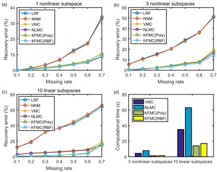
We randomly remove some portions of the entries of the matrices and use matrix completion to recover the missing entries. The performances are evaluated by the relative error defined as RE=𝑿^𝑿F/𝑿F𝑅𝐸subscriptnorm^𝑿𝑿𝐹subscriptnorm𝑿𝐹RE=\|\widehat{\bm{X}}-\bm{X}\|_{F}/\|\bm{X}\|_{F} [6], where 𝑿^^𝑿\widehat{\bm{X}} denotes the recovered matrix. As shown in Figure 1, the recovery errors of LRMC methods, i.e. LRF [27] and NNM [4], are considerably high. In contrast, HRMC methods especially our KFMC have significantly lower recovery errors. In addition, our KFMC(Poly) and KFMC(RBF) are much more efficient than VMC [25] and NLMC [10], in which randomized SVD [12] has been performed.

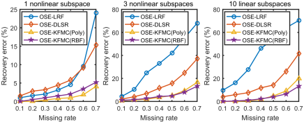
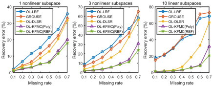
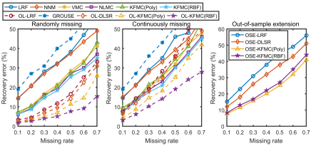
Figure 2 shows the results of online matrix completion, in which OL-DLSR (dictionary learning and sparse representation) is an online matrix completion method we modified from [22] and [11] and detailed in our supplementary material. We see that our method OL-KFMC outperformed other methods significantly. Figures 3 shows the results of out-of-sample extension (OSE) of HRMC, in which our OSE-KFMC outperformed other methods. More details about the experiment/parameter settings and analysis are in the supplementary material.
Refer to caption
Figure 1: Offline matrix completion on synthetic data
Refer to caption
Figure 2: Online matrix completion on synthetic data
Refer to caption
Figure 3: Out-of-sample extension of matrix completion on synthetic data

4.2 Hopkins155 data

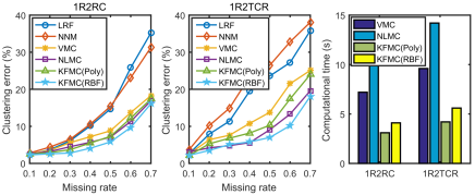
Similar to [25], we consider the problem of subspace clustering on incomplete data, in which the missing data of Hopkins155 [28] were recovered by matrix completion and then SSC (sparse subspace clustering [7]) was performed. We consider two downsampled video sequences, 1R2RC and 1R2TCR, each of which consists of 6 frames. The average clustering errors [7] of 10 repeated trials are reported in Figure 4. Our method KFMC with RBF kernel is more accurate and efficient than VMC and NLMC.
Refer to caption
Figure 4: Subspace clustering on incomplete data

4.3 CMU motion capture data

We use matrix completion to recover the missing data of time-series trajectories of human motions (e.g. running and jumping). Similar to [6, 25], we use the trial #6#6\#6 of subject #56#56\#56 of the CMU motion capture dataset, which forms a high rank matrix [6]. We consider two cases of incomplete data, randomly missing and continuously missing. More details about the experimental settings are in the supplementary material. The average results of 10 repeated trials are reported in Figure 5. We see that HRMC methods outperformed LRMC methods while online methods outperformed offline methods. One reason is that the structure of the data changes with time (corresponding to different motions) and online methods can adapt to the changes. Comparing Figure 5 with the Figure 4 of [6], we find that VMC, NLMC, and our KFMC outperformed the method proposed in [6]. In addition, our OL-KFMC especially with RBF kernel is the most accurate one. Regarding the computational cost, there is no doubt that the linear methods including LRF, NNM, GROUSE, and DLSR are faster than other methods. Hence we only show the computational cost of the nonlinear methods in Table 2 for comparison (randomized SVD [12] has been performed in VMC and NLMC). Our KFMC is faster than VMC and NLMC while our OL-KFMC is at least 10 times faster than all methods.
Refer to caption
Figure 5: CMU motion capture data recovery
VMC   370 NLMC      610 KFMC(Poly)     170
KFMC(RBF)  190 OL-KFMC(Poly)  16 OL-KFMC(RBF)  19
Table 2: Time cost (second) on CMU motion capture data

5 Conclusion

In this paper, we proposed kernelized factorization matrix completion (KFMC)111The codes are available at https://github.com/jicongfan/Online-high-rank-matrix-completion, a new method for high rank matrix completion, together with an online version and an out-of-sample extension, which outperform state-of-the-art methods. Our numerics demonstrate the success of the method for motion data recovery. We believe our methods will also be useful for transductive learning (classification), vehicle/robot/chemistry sensor signal denoising, recommender systems, and biomedical data recovery.

Acknowledgement

This work was supported in part by DARPA Award FA8750-17-2-0101.

References

  • [1] Xavier Alameda-Pineda, Elisa Ricci, Yan Yan, and Nicu Sebe. Recognizing emotions from abstract paintings using non-linear matrix completion. In Proceedings of the IEEE Conference on Computer Vision and Pattern Recognition, pages 5240–5248, 2016.
  • [2] Laura Balzano, Robert Nowak, and Benjamin Recht. Online identification and tracking of subspaces from highly incomplete information. In Communication, Control, and Computing (Allerton), 2010 48th Annual Allerton Conference on, pages 704–711. IEEE, 2010.
  • [3] Srinadh Bhojanapalli and Prateek Jain. Universal matrix completion. In Proceedings of The 31st International Conference on Machine Learning, pages 1881–1889. JMLR, 2014.
  • [4] Emmanuel J. Candès and Benjamin Recht. Exact matrix completion via convex optimization. Foundations of Computational Mathematics, 9(6):717–772, 2009.
  • [5] Charanpal Dhanjal, Romaric Gaudel, and Stéphan Clémençon. Online matrix completion through nuclear norm regularisation. In Proceedings of the 2014 SIAM International Conference on Data Mining, pages 623–631. SIAM, 2014.
  • [6] Ehsan Elhamifar. High-rank matrix completion and clustering under self-expressive models. In Advances in Neural Information Processing Systems 29, pages 73–81, 2016.
  • [7] E. Elhamifar and R. Vidal. Sparse subspace clustering: Algorithm, theory, and applications. IEEE Transactions on Pattern Analysis and Machine Intelligence, 35(11):2765–2781, 2013.
  • [8] Brian Eriksson, Laura Balzano, and Robert Nowak. High-rank matrix completion. In Artificial Intelligence and Statistics, pages 373–381, 2012.
  • [9] Jicong Fan and Tommy W.S. Chow. Matrix completion by least-square, low-rank, and sparse self-representations. Pattern Recognition, 71:290 – 305, 2017.
  • [10] Jicong Fan and Tommy W.S. Chow. Non-linear matrix completion. Pattern Recognition, 77:378 – 394, 2018.
  • [11] J. Fan, M. Zhao, and T. W. S. Chow. Matrix completion via sparse factorization solved by accelerated proximal alternating linearized minimization. IEEE Transactions on Big Data, pages 1–1, 2018.
  • [12] N. Halko, P. G. Martinsson, and J. A. Tropp. Finding structure with randomness: Probabilistic algorithms for constructing approximate matrix decompositions. SIAM Review, 53(2):217–288, 2011.
  • [13] Moritz Hardt. Understanding alternating minimization for matrix completion. In Foundations of Computer Science (FOCS), 2014 IEEE 55th Annual Symposium on, pages 651–660. IEEE, 2014.
  • [14] Chi Jin, Sham M Kakade, and Praneeth Netrapalli. Provable efficient online matrix completion via non-convex stochastic gradient descent. In Advances in Neural Information Processing Systems, pages 4520–4528, 2016.
  • [15] Jaya Kawale, Hung H Bui, Branislav Kveton, Long Tran-Thanh, and Sanjay Chawla. Efficient thompson sampling for online matrix-factorization recommendation. In Advances in neural information processing systems, pages 1297–1305, 2015.
  • [16] R. H. Keshavan, A. Montanari, and S. Oh. Matrix completion from a few entries. IEEE Transactions on Information Theory, 56(6):2980–2998, June 2010.
  • [17] Chun-Guang Li and Rene Vidal. A structured sparse plus structured low-rank framework for subspace clustering and completion. IEEE Transactions on Signal Processing, 64(24):6557–6570, 2016.
  • [18] Zhouchen Lin, Minming Chen, and Yi Ma. The augmented lagrange multiplier method for exact recovery of corrupted low-rank matrices. arXiv:1009.5055v3 [math.OC], 2010.
  • [19] Guangcan Liu and Ping Li. Low-rank matrix completion in the presence of high coherence. IEEE Transactions on Signal Processing, 64(21):5623–5633, 2016.
  • [20] Brian Lois and Namrata Vaswani. Online matrix completion and online robust pca. In Information Theory (ISIT), 2015 IEEE International Symposium on, pages 1826–1830. IEEE, 2015.
  • [21] C. Lu, J. Tang, S. Yan, and Z. Lin. Generalized nonconvex nonsmooth low-rank minimization. In 2014 IEEE Conference on Computer Vision and Pattern Recognition, pages 4130–4137, June 2014.
  • [22] Julien Mairal, Francis Bach, Jean Ponce, and Guillermo Sapiro. Online dictionary learning for sparse coding. In Proceedings of the 26th annual international conference on machine learning, pages 689–696. ACM, 2009.
  • [23] Rahul Mazumder, Trevor Hastie, and Robert Tibshirani. Spectral regularization algorithms for learning large incomplete matrices. Journal of machine learning research, 11(Aug):2287–2322, 2010.
  • [24] Feiping Nie, Heng Huang, and Chris Ding. Low-rank matrix recovery via efficient schatten p-norm minimization. In Proceedings of the Twenty-Sixth AAAI Conference on Artificial Intelligence, pages 655–661. AAAI Press, 2012.
  • [25] Greg Ongie, Rebecca Willett, Robert D. Nowak, and Laura Balzano. Algebraic variety models for high-rank matrix completion. In Proceedings of the 34th International Conference on Machine Learning, pages 2691–2700. PMLR, 2017.
  • [26] Steffen Rendle and Lars Schmidt-Thieme. Online-updating regularized kernel matrix factorization models for large-scale recommender systems. In Proceedings of the 2008 ACM conference on Recommender systems, pages 251–258. ACM, 2008.
  • [27] Ruoyu Sun and Zhi-Quan Luo. Guaranteed matrix completion via non-convex factorization. IEEE Transactions on Information Theory, 62(11):6535–6579, 2016.
  • [28] R. Tron and R. Vidal. A benchmark for the comparison of 3-d motion segmentation algorithms. In 2007 IEEE Conference on Computer Vision and Pattern Recognition, pages 1–8, June 2007.
  • [29] Congyuan Yang, Daniel Robinson, and Rene Vidal. Sparse subspace clustering with missing entries. In International Conference on Machine Learning, pages 2463–2472, 2015.
  • [30] Se-Young Yun, Marc Lelarge, and Alexandre Proutiere. Streaming, memory limited matrix completion with noise. arXiv preprint arXiv:1504.03156, 2015.

Appendix

Appendix A Proof of some lemmas

A.1 Proof for Lemma 3

Lemma 3. The update (8) is a relaxed Newton’s method and ensures sufficient decrease in the objective:

(𝒁,𝑫𝚫𝑫,𝑿)(𝒁,𝑫,𝑿)12τTr(𝒈𝑫𝑯𝑫1𝒈𝑫).𝒁𝑫subscript𝚫𝑫𝑿𝒁𝑫𝑿12𝜏Trsubscript𝒈𝑫superscriptsubscript𝑯𝑫1superscriptsubscript𝒈𝑫top\ell(\bm{Z},\bm{D}-\bm{\Delta}_{\scalebox{0.6}{$\bm{D}$}},\bm{X})-\ell(\bm{Z},\bm{D},\bm{X})\leq-\tfrac{1}{2\tau}\textup{Tr}(\bm{g}_{\scalebox{0.6}{$\bm{D}$}}\bm{H}_{\scalebox{0.6}{$\bm{D}$}}^{-1}\bm{g}_{\scalebox{0.6}{$\bm{D}$}}^{\top}).
Proof.

With polynomial kernel, the objective function in terms of 𝑫𝑫\bm{D} is

(𝒁,𝑫,𝑿)=𝒁𝑫𝑿absent\displaystyle\ell(\bm{Z},\bm{D},\bm{X})= Tr((𝑾1(𝑿T𝑫+c))𝒁)Trdirect-productsubscript𝑾1superscript𝑿𝑇𝑫𝑐𝒁\displaystyle-\text{Tr}((\bm{W}_{1}\odot(\bm{X}^{T}\bm{D}+c))\bm{Z}) (40)
+12Tr(𝒁T(𝑾2(𝑫T𝑫+c))𝒁)12Trsuperscript𝒁𝑇direct-productsubscript𝑾2superscript𝑫𝑇𝑫𝑐𝒁\displaystyle+\tfrac{1}{2}\text{Tr}(\bm{Z}^{T}(\bm{W}_{2}\odot(\bm{D}^{T}\bm{D}+c))\bm{Z})
+α2Tr(𝑾2(𝑫T𝑫+c)),𝛼2Trdirect-productsubscript𝑾2superscript𝑫𝑇𝑫𝑐\displaystyle+\tfrac{\alpha}{2}\text{Tr}(\bm{W}_{2}\odot(\bm{D}^{T}\bm{D}+c)),

in which for simplicity we have omitted the terms not related to 𝑫𝑫\bm{D}. In (40), 𝑾1=𝑿T𝑫+cq1subscript𝑾1superscriptdelimited-⟨⟩superscript𝑿𝑇𝑫𝑐𝑞1\bm{W}_{1}=\langle\bm{X}^{T}\bm{D}+c\rangle^{q-1}, 𝑾2=𝑫T𝑫+cq1subscript𝑾2superscriptdelimited-⟨⟩superscript𝑫𝑇𝑫𝑐𝑞1\bm{W}_{2}=\langle\bm{D}^{T}\bm{D}+c\rangle^{q-1}, and usuperscriptdelimited-⟨⟩𝑢\langle\cdot\rangle^{u} denotes the element-wise u𝑢u-power of a vector or matrix. Using the idea of iteratively reweighted optimization, we fix 𝑾1subscript𝑾1\bm{W}_{1} and 𝑾2subscript𝑾2\bm{W}_{2}, and get the derivative as

𝒈𝑫:=𝑿(𝑾1𝒁T)+𝑫(𝒁𝒁T𝑾2)+α𝑫(𝑾2𝑰r)).\bm{g}_{\scalebox{0.6}{$\bm{D}$}}:=-\bm{X}(\bm{W}_{1}\odot\bm{Z}^{T})+\bm{D}(\bm{Z}\bm{Z}^{T}\odot\bm{W}_{2})+\alpha\bm{D}(\bm{W}_{2}\odot\bm{I}_{r})). (41)

We approximate (𝒁,𝑫,𝑿)𝒁𝑫𝑿\ell(\bm{Z},\bm{D},\bm{X}) with its second order Taylor expansion around 𝑫0subscript𝑫0\bm{D}_{0}, i.e.,

(𝒁,𝑫,𝑿)=𝒁𝑫𝑿absent\displaystyle\ell(\bm{Z},\bm{D},\bm{X})= (𝒁,𝑫0,𝑿)+𝒈𝑫,𝑫𝑫0𝒁subscript𝑫0𝑿subscript𝒈𝑫𝑫subscript𝑫0\displaystyle\ell(\bm{Z},\bm{D}_{0},\bm{X})+\langle\bm{g}_{\scalebox{0.6}{$\bm{D}$}},\bm{D}-\bm{D}_{0}\rangle (42)
+12vec(𝑫𝑫0)T𝑯𝑫vec(𝑫𝑫0)+R0,12vecsuperscript𝑫subscript𝑫0𝑇subscript𝑯𝑫vec𝑫subscript𝑫0subscript𝑅0\displaystyle+\tfrac{1}{2}\mbox{vec}(\bm{D}-\bm{D}_{0})^{T}\bm{H}_{\scalebox{0.6}{$\bm{D}$}}\mbox{vec}(\bm{D}-\bm{D}_{0})+R_{0},

where R0=O((3)6)subscript𝑅0𝑂normsuperscript36R_{0}=O(\tfrac{\|\ell^{(3)}\|}{6}) denotes the residual of the approximation and 𝑯r2×r2𝑯superscriptsuperscript𝑟2superscript𝑟2\bm{H}\in\mathbb{R}^{r^{2}\times r^{2}} denotes the Hessian matrix. We have

𝑯=[𝑯𝑫𝟎𝟎𝟎𝑯𝑫𝟎𝟎𝟎𝑯𝑫],𝑯delimited-[]matrixsubscript𝑯𝑫000subscript𝑯𝑫000subscript𝑯𝑫\bm{H}=\left[\begin{matrix}\bm{H}_{\scalebox{0.6}{$\bm{D}$}}&\bm{0}&\cdots&\bm{0}\\ \bm{0}&\bm{H}_{\scalebox{0.6}{$\bm{D}$}}&\cdots&\bm{0}\\ \vdots&\cdots&\ddots&\vdots\\ \bm{0}&\bm{0}&\cdots&\bm{H}_{\scalebox{0.6}{$\bm{D}$}}\end{matrix}\right], (43)

where

𝑯𝑫:=𝒁𝒁T𝑾2+α𝑾2𝑰r.assignsubscript𝑯𝑫direct-product𝒁superscript𝒁𝑇subscript𝑾2direct-product𝛼subscript𝑾2subscript𝑰𝑟\bm{H}_{\scalebox{0.6}{$\bm{D}$}}:=\bm{Z}\bm{Z}^{T}\odot\bm{W}_{2}+\alpha\bm{W}_{2}\odot\bm{I}_{r}. (44)

One has vec(𝑫𝑫0)T𝑯vec(𝑫𝑫0)=Tr((𝑫𝑫𝟎)𝑯(𝑫𝑫𝟎)T)vecsuperscript𝑫subscript𝑫0𝑇𝑯vec𝑫subscript𝑫0Tr𝑫subscript𝑫0𝑯superscript𝑫subscript𝑫0𝑇\mbox{vec}(\bm{D}-\bm{D}_{0})^{T}\bm{H}\mbox{vec}(\bm{D}-\bm{D}_{0})=\text{Tr}((\bm{D}-\bm{{D}_{0}})\bm{H}(\bm{D}-\bm{{D}_{0}})^{T}). Denote

(𝒁,𝑫,𝑿)=superscript𝒁𝑫𝑿absent\displaystyle\ell^{\prime}(\bm{Z},\bm{D},\bm{X})= (𝒁,𝑫0,𝑿)+𝒈𝑫,𝑫𝑫0𝒁subscript𝑫0𝑿subscript𝒈𝑫𝑫subscript𝑫0\displaystyle\ell(\bm{Z},\bm{D}_{0},\bm{X})+\langle\bm{g}_{\scalebox{0.6}{$\bm{D}$}},\bm{D}-\bm{D}_{0}\rangle (45)
+\displaystyle+ τ2Tr((𝑫𝑫𝟎)𝑯𝑫(𝑫𝑫𝟎)T),𝜏2Tr𝑫subscript𝑫0subscript𝑯𝑫superscript𝑫subscript𝑫0𝑇\displaystyle\tfrac{\tau}{2}\text{Tr}((\bm{D}-\bm{{D}_{0}})\bm{H}_{\scalebox{0.6}{$\bm{D}$}}(\bm{D}-\bm{{D}_{0}})^{T}),

where τ>1𝜏1\tau>1. Since 𝑯𝑫subscript𝑯𝑫\bm{H}_{\scalebox{0.6}{$\bm{D}$}} is positive definite, we have

(𝒁,𝑫,𝑿)(𝒁,𝑫,𝑿),𝒁𝑫𝑿superscript𝒁𝑫𝑿\ell(\bm{Z},\bm{D},\bm{X})\leq\ell^{\prime}(\bm{Z},\bm{D},\bm{X}), (46)

provided that τ𝜏\tau is large enough. We then minimize superscript\ell^{\prime} by letting the derivative be zero and get

𝑫=𝑫0𝚫𝑫.𝑫subscript𝑫0subscript𝚫𝑫\bm{D}=\bm{D}_{0}-\bm{\Delta}_{\scalebox{0.6}{$\bm{D}$}}. (47)

where 𝚫𝑫=1τ𝒈𝑫𝑯𝑫1subscript𝚫𝑫1𝜏subscript𝒈𝑫superscriptsubscript𝑯𝑫1\bm{\Delta}_{\scalebox{0.6}{$\bm{D}$}}=\tfrac{1}{\tau}\bm{g}_{\scalebox{0.6}{$\bm{D}$}}\bm{H}_{\scalebox{0.6}{$\bm{D}$}}^{-1}. Invoking (47) into (46), we have

(𝒁,𝑫0𝚫𝑫,𝑿)(𝒁,𝑫0,𝑿)12τTr(𝒈𝑫𝑯𝑫1𝒈𝑫T).𝒁subscript𝑫0subscript𝚫𝑫𝑿𝒁subscript𝑫0𝑿12𝜏Trsubscript𝒈𝑫superscriptsubscript𝑯𝑫1superscriptsubscript𝒈𝑫𝑇\ell(\bm{Z},\bm{D}_{0}-\bm{\Delta}_{\scalebox{0.6}{$\bm{D}$}},\bm{X})\leq\ell(\bm{Z},\bm{D}_{0},\bm{X})-\tfrac{1}{2\tau}\text{Tr}(\bm{g}_{\scalebox{0.6}{$\bm{D}$}}\bm{H}_{\scalebox{0.6}{$\bm{D}$}}^{-1}\bm{g}_{\scalebox{0.6}{$\bm{D}$}}^{T}). (48)

A.2 Proof for Lemma 4

Lemma 4. 𝑿(𝒁T𝑲𝑿𝑫1)𝑿(𝒁T𝑲𝑿𝑫2)Fcσn𝑿2𝑫1𝑫2Fsubscriptnorm𝑿direct-productsuperscript𝒁𝑇subscript𝑲𝑿subscript𝑫1𝑿direct-productsuperscript𝒁𝑇subscript𝑲𝑿subscript𝑫2𝐹𝑐𝜎𝑛subscriptnorm𝑿2subscriptnormsubscript𝑫1subscript𝑫2𝐹\|\bm{X}(\bm{Z}^{T}\odot\bm{K}_{\scalebox{0.6}{$\bm{X}\bm{D}_{1}$}})-\bm{X}(\bm{Z}^{T}\odot\bm{K}_{\scalebox{0.6}{$\bm{X}\bm{D}_{2}$}})\|_{F}\leq\tfrac{c}{\sigma\sqrt{n}}\|\bm{X}\|_{2}\|\bm{D}_{1}-\bm{D}_{2}\|_{F}, where c𝑐c is a small constant.

Proof.

Since 𝒁=min𝒁12ϕ(𝑿)ϕ(𝑫)𝒁F2+β2𝒁F2𝒁subscript𝒁12superscriptsubscriptnormitalic-ϕ𝑿italic-ϕ𝑫𝒁𝐹2𝛽2superscriptsubscriptnorm𝒁𝐹2\bm{Z}=\min\limits_{\bm{Z}}\tfrac{1}{2}\|\phi(\bm{X})-\phi(\bm{D})\bm{Z}\|_{F}^{2}+\tfrac{\beta}{2}\|\bm{Z}\|_{F}^{2}, we have

𝒁=(ϕ(𝑫)Tϕ(𝑫)+β𝑰r)1ϕ(𝑫)Tϕ(𝑿).𝒁superscriptitalic-ϕsuperscript𝑫𝑇italic-ϕ𝑫𝛽subscript𝑰𝑟1italic-ϕsuperscript𝑫𝑇italic-ϕ𝑿\bm{Z}=(\phi(\bm{D})^{T}\phi(\bm{D})+\beta\bm{I}_{r})^{-1}\phi(\bm{D})^{T}\phi(\bm{X}). (49)

Denote ϕ(𝑫)=𝑼𝑺𝑽T=𝑼diag(λ1,,λr)𝑽Titalic-ϕ𝑫𝑼𝑺superscript𝑽𝑇𝑼diagsubscript𝜆1subscript𝜆𝑟superscript𝑽𝑇\phi(\bm{D})=\bm{U}\bm{S}\bm{V}^{T}=\bm{U}\text{diag}(\lambda_{1},\cdots,\lambda_{r})\bm{V}^{T} (the singular value decomposition), we have ϕ(𝑿)=𝑼𝑺^𝑽^T=𝑼diag(λ^1,,λ^r)𝑽^Titalic-ϕ𝑿𝑼^𝑺superscript^𝑽𝑇𝑼diagsubscript^𝜆1subscript^𝜆𝑟superscript^𝑽𝑇\phi(\bm{X})=\bm{U}\hat{\bm{S}}\hat{\bm{V}}^{T}=\bm{U}\text{diag}(\hat{\lambda}_{1},\cdots,\hat{\lambda}_{r})\hat{\bm{V}}^{T} because ϕ(𝑿)italic-ϕ𝑿\phi(\bm{X}) and ϕ(𝑫)italic-ϕ𝑫\phi(\bm{D}) have the same column basis. Then

𝒁=𝒁absent\displaystyle\bm{Z}= 𝑽(𝑺2+β𝑰)1𝑺𝑺^𝑽^T𝑽superscriptsuperscript𝑺2𝛽𝑰1𝑺^𝑺superscript^𝑽𝑇\displaystyle\bm{V}(\bm{S}^{2}+\beta\bm{I})^{-1}\bm{S}\hat{\bm{S}}\hat{\bm{V}}^{T} (50)
=𝑽diag(λ1λ^1λ12+β,,λrλ^rλr2+β)𝑽^T.absent𝑽diagsubscript𝜆1subscript^𝜆1superscriptsubscript𝜆12𝛽subscript𝜆𝑟subscript^𝜆𝑟superscriptsubscript𝜆𝑟2𝛽superscript^𝑽𝑇\displaystyle=\bm{V}\text{diag}(\tfrac{\lambda_{1}\hat{\lambda}_{1}}{\lambda_{1}^{2}+\beta},\cdots,\tfrac{\lambda_{r}\hat{\lambda}_{r}}{\lambda_{r}^{2}+\beta})\hat{\bm{V}}^{T}.

Suppose β𝛽\beta is large enough, we have λiλ^iλi2+β<1subscript𝜆𝑖subscript^𝜆𝑖superscriptsubscript𝜆𝑖2𝛽1\tfrac{\lambda_{i}\hat{\lambda}_{i}}{\lambda_{i}^{2}+\beta}<1 for i=1,,r𝑖1𝑟i=1,\cdots,r. It follows that 𝒁F2<rsuperscriptsubscriptnorm𝒁𝐹2𝑟\|\bm{Z}\|_{F}^{2}<r and E[zij2]<1n𝐸delimited-[]superscriptsubscript𝑧𝑖𝑗21𝑛E[z_{ij}^{2}]<\tfrac{1}{n}, which indicates that

{σz=E[|zijμz|]<1n,1n<μz=E[zij]<1n.\left\{\begin{matrix}\sigma_{z}=E[|z_{ij}-\mu_{z}|]<\tfrac{1}{\sqrt{n}},\\ -\tfrac{1}{\sqrt{n}}<\mu_{z}=E[z_{ij}]<\tfrac{1}{\sqrt{n}}.\end{matrix}\right. (51)

According to Chebyshev’s inequality, we have

Pr(|zij|>c0n+1n)<1c02.Prsubscript𝑧𝑖𝑗subscript𝑐0𝑛1𝑛1superscriptsubscript𝑐02\text{Pr}(|z_{ij}|>\tfrac{c_{0}}{\sqrt{n}}+\tfrac{1}{\sqrt{n}})<\tfrac{1}{c_{0}^{2}}. (52)

Therefore, |zij|<c0nsubscript𝑧𝑖𝑗subscript𝑐0𝑛|z_{ij}|<\tfrac{c_{0}}{\sqrt{n}} holds with high probability provided that c0subscript𝑐0c_{0} is large enough. Suppose zij𝒩(μz,σz2)similar-tosubscript𝑧𝑖𝑗𝒩subscript𝜇𝑧superscriptsubscript𝜎𝑧2z_{ij}\sim\mathcal{N}(\mu_{z},\sigma_{z}^{2}), we have

Pr(|zij|>c0n)<e0.5c02Prsubscript𝑧𝑖𝑗subscript𝑐0𝑛superscript𝑒0.5superscriptsubscript𝑐02\text{Pr}(|z_{ij}|>\tfrac{c_{0}}{\sqrt{n}})<e^{-0.5c_{0}^{2}} (53)

according to the upper bound of Q-function of normal distribution. Then using union bound, we obtain

Pr(|zij|<c0n,(i,j))<1nre0.5c02,Prsubscript𝑧𝑖𝑗subscript𝑐0𝑛for-all𝑖𝑗1𝑛𝑟superscript𝑒0.5superscriptsubscript𝑐02\text{Pr}\big{(}|z_{ij}|<\tfrac{c_{0}}{\sqrt{n}},\forall(i,j)\big{)}<1-nre^{-0.5c_{0}^{2}}, (54)

It is equivalent to

Pr(|zij|<c1n,(i,j))<11(nr)c01,Prsubscript𝑧𝑖𝑗subscript𝑐1𝑛for-all𝑖𝑗11superscript𝑛𝑟subscript𝑐01\text{Pr}\big{(}|z_{ij}|<\tfrac{c_{1}}{\sqrt{n}},\forall(i,j)\big{)}<1-\tfrac{1}{(nr)^{c_{0}-1}}, (55)

where c1=2c0log(nr)subscript𝑐12subscript𝑐0𝑛𝑟c_{1}=\sqrt{2c_{0}\log(nr)}.

On the other hand, the partial gradient of entry (i,j)𝑖𝑗(i,j) of 𝑲𝑿𝑫subscript𝑲𝑿𝑫\bm{K}_{\scalebox{0.6}{$\bm{X}\bm{D}$}} in terms of 𝑫:jsubscript𝑫:absent𝑗\bm{D}_{:j} (the j𝑗j-th column of 𝑫𝑫\bm{D}) can be given by

𝑲𝑿𝑫(i,j)𝑫:j=1σ2(𝑿:i𝑫:j)exp(𝑿:i𝑫:j22σ2).subscript𝑲𝑿𝑫𝑖𝑗subscript𝑫:absent𝑗1superscript𝜎2subscript𝑿:absent𝑖subscript𝑫:absent𝑗superscriptnormsubscript𝑿:absent𝑖subscript𝑫:absent𝑗22superscript𝜎2\tfrac{\partial\bm{K}_{\scalebox{0.6}{$\bm{X}\bm{D}$}}(i,j)}{\partial\bm{D}_{:j}}=-\tfrac{1}{\sigma^{2}}(\bm{X}_{:i}-\bm{D}_{:j})\exp(-\tfrac{\|\bm{X}_{:i}-\bm{D}_{:j}\|^{2}}{2\sigma^{2}}). (56)

Because |xexp(x22σ2)|σexp(0.5)<0.61σ𝑥superscript𝑥22superscript𝜎2𝜎0.50.61𝜎|x\exp(\tfrac{-x^{2}}{2\sigma^{2}})|\leq\sigma\exp(-0.5)<0.61\sigma, we have |𝑲𝑿𝑫(i,j)𝑫kj|<c2σsubscript𝑲𝑿𝑫𝑖𝑗subscript𝑫𝑘𝑗subscript𝑐2𝜎|\tfrac{\partial\bm{K}_{\scalebox{0.6}{$\bm{X}\bm{D}$}}(i,j)}{\partial\bm{D}_{kj}}|<\tfrac{c_{2}}{\sigma} for some constant c2subscript𝑐2c_{2}. Then

𝑲𝑿𝑫1𝑲𝑿𝑫2Fc3σ𝑫1𝑫2Fsubscriptnormsubscript𝑲𝑿subscript𝑫1subscript𝑲𝑿subscript𝑫2𝐹subscript𝑐3𝜎subscriptnormsubscript𝑫1subscript𝑫2𝐹\|\bm{K}_{\scalebox{0.6}{$\bm{X}\bm{D}_{1}$}}-\bm{K}_{\scalebox{0.6}{$\bm{X}\bm{D}_{2}$}}\|_{F}\leq\tfrac{c_{3}}{\sigma}\|\bm{D}_{1}-\bm{D}_{2}\|_{F} (57)

some small constant c3subscript𝑐3c_{3}.

According to the above analysis, we get

𝑿(𝒁T𝑲𝑿𝑫1)𝑿(𝒁T𝑲𝑿𝑫2)Fsubscriptnorm𝑿direct-productsuperscript𝒁𝑇subscript𝑲𝑿subscript𝑫1𝑿direct-productsuperscript𝒁𝑇subscript𝑲𝑿subscript𝑫2𝐹\displaystyle\|\bm{X}(\bm{Z}^{T}\odot\bm{K}_{\scalebox{0.6}{$\bm{X}\bm{D}_{1}$}})-\bm{X}(\bm{Z}^{T}\odot\bm{K}_{\scalebox{0.6}{$\bm{X}\bm{D}_{2}$}})\|_{F} (58)
\displaystyle\leq 𝑿2𝒁T(𝑲𝑿𝑫1𝑲𝑿𝑫2)Fsubscriptnorm𝑿2subscriptnormdirect-productsuperscript𝒁𝑇subscript𝑲𝑿subscript𝑫1subscript𝑲𝑿subscript𝑫2𝐹\displaystyle\|\bm{X}\|_{2}\|\bm{Z}^{T}\odot(\bm{K}_{\scalebox{0.6}{$\bm{X}\bm{D}_{1}$}}-\bm{K}_{\scalebox{0.6}{$\bm{X}\bm{D}_{2}$}})\|_{F}
\displaystyle\leq c1n𝑿2𝑲𝑿𝑫1𝑲𝑿𝑫2Fsubscript𝑐1𝑛subscriptnorm𝑿2subscriptnormsubscript𝑲𝑿subscript𝑫1subscript𝑲𝑿subscript𝑫2𝐹\displaystyle\tfrac{c_{1}}{\sqrt{n}}\|\bm{X}\|_{2}\|\bm{K}_{\scalebox{0.6}{$\bm{X}\bm{D}_{1}$}}-\bm{K}_{\scalebox{0.6}{$\bm{X}\bm{D}_{2}$}}\|_{F}
\displaystyle\leq c1nc3σ𝑿2𝑫1𝑫2Fsubscript𝑐1𝑛subscript𝑐3𝜎subscriptnorm𝑿2subscriptnormsubscript𝑫1subscript𝑫2𝐹\displaystyle\tfrac{c_{1}}{\sqrt{n}}\tfrac{c_{3}}{\sigma}\|\bm{X}\|_{2}\|\bm{D}_{1}-\bm{D}_{2}\|_{F}
=\displaystyle= cσn𝑿2𝑫1𝑫2F.𝑐𝜎𝑛subscriptnorm𝑿2subscriptnormsubscript𝑫1subscript𝑫2𝐹\displaystyle\tfrac{c}{\sigma\sqrt{n}}\|\bm{X}\|_{2}\|\bm{D}_{1}-\bm{D}_{2}\|_{F}.

A.3 Proof for Lemma 5

Lemma 5. For sufficiently small η𝜂\eta, Algorithm 1 converges to a stationary point.

Proof.

Denote the objective function of (7) by (𝒁,𝑫,𝑿)𝒁𝑫𝑿\ell(\bm{Z},\bm{D},\bm{X}), which is lower-bounded by at least 0. When η=0𝜂0\eta=0, as the three subproblems are well addressed and do not diverge, we have (𝒁t+1,𝑫t+1,𝑿t+1)<(𝒁t+1,𝑫t+1,𝑿t)<(𝒁t+1,𝑫t,𝑿t)<(𝒁t,𝑫t,𝑿t)subscript𝒁𝑡1subscript𝑫𝑡1subscript𝑿𝑡1subscript𝒁𝑡1subscript𝑫𝑡1subscript𝑿𝑡subscript𝒁𝑡1subscript𝑫𝑡subscript𝑿𝑡subscript𝒁𝑡subscript𝑫𝑡subscript𝑿𝑡\ell(\bm{Z}_{t+1},\bm{D}_{t+1},\bm{X}_{t+1})<\ell(\bm{Z}_{t+1},\bm{D}_{t+1},\bm{X}_{t})<\ell(\bm{Z}_{t+1},\bm{D}_{t},\bm{X}_{t})<\ell(\bm{Z}_{t},\bm{D}_{t},\bm{X}_{t}). It indicates that Δt=(𝒁t,𝑫t,𝑿t)(𝒁t+1,𝑫t+1,𝑿t+1)0subscriptΔ𝑡subscript𝒁𝑡subscript𝑫𝑡subscript𝑿𝑡subscript𝒁𝑡1subscript𝑫𝑡1subscript𝑿𝑡10\Delta_{t}=\ell(\bm{Z}_{t},\bm{D}_{t},\bm{X}_{t})-\ell(\bm{Z}_{t+1},\bm{D}_{t+1},\bm{X}_{t+1})\rightarrow 0 when t𝑡t\rightarrow\infty. When Δt=0subscriptΔ𝑡0\Delta_{t}=0, the gradient of (𝒁t,𝑫t,𝑿t)subscript𝒁𝑡subscript𝑫𝑡subscript𝑿𝑡\ell(\bm{Z}_{t},\bm{D}_{t},\bm{X}_{t}) is 0. Then Algorithm 1 converges to a stationary point.

When η>0𝜂0\eta>0 and take 𝑫𝑫\bm{D} as an example, because 𝚫D,tsubscript𝚫𝐷𝑡\bm{\Delta}_{D,t} is not exact enough, we decompose 𝚫D,tsubscript𝚫𝐷𝑡\bm{\Delta}_{D,t} as 𝚫D,t=ct𝚫D,t+𝚫D,tsubscript𝚫𝐷𝑡subscript𝑐𝑡superscriptsubscript𝚫𝐷𝑡superscriptsubscript𝚫𝐷𝑡\bm{\Delta}_{D,t}=c_{t}\bm{\Delta}_{D,t}^{*}+\bm{\Delta}_{D,t}^{\prime}, where 0<ct<10subscript𝑐𝑡10<c_{t}<1 and 𝚫D,tsuperscriptsubscript𝚫𝐷𝑡\bm{\Delta}_{D,t}^{*} is nearly optimal at iteration t𝑡t. Similarly, we have 𝚫D,t1=ct1𝚫D,t+𝚫D,t1subscript𝚫𝐷𝑡1subscript𝑐𝑡1superscriptsubscript𝚫𝐷𝑡superscriptsubscript𝚫𝐷𝑡1\bm{\Delta}_{D,t-1}=c_{t-1}\bm{\Delta}_{D,t}^{*}+\bm{\Delta}_{D,t-1}^{\prime}. Then 𝚫^t=(ct+ct1η++c0ηt)𝚫D,t+ϵsubscript^𝚫𝑡subscript𝑐𝑡subscript𝑐𝑡1𝜂subscript𝑐0superscript𝜂𝑡superscriptsubscript𝚫𝐷𝑡superscriptbold-italic-ϵ\widehat{\bm{\Delta}}_{t}=(c_{t}+c_{t-1}\eta+\cdots+c_{0}\eta^{t})\bm{\Delta}_{D,t}^{*}+\bm{\epsilon}^{\prime}, where ϵ=i=0tηi𝚫D,isuperscriptbold-italic-ϵsuperscriptsubscript𝑖0𝑡superscript𝜂𝑖superscriptsubscript𝚫𝐷𝑖\bm{\epsilon}^{\prime}=\sum_{i=0}^{t}\eta^{i}\bm{\Delta}_{D,i}^{\prime}. ϵsuperscriptbold-italic-ϵ\bm{\epsilon}^{\prime} could be small compared to 𝚫D,tsuperscriptsubscript𝚫𝐷𝑡\bm{\Delta}_{D,t}^{\prime} because the signs of elements of 𝚫D,0,,𝚫D,tsuperscriptsubscript𝚫𝐷0superscriptsubscript𝚫𝐷𝑡\bm{\Delta}_{D,0}^{\prime},\cdots,\bm{\Delta}_{D,t}^{\prime} may change. Suppose ctsubscript𝑐𝑡c_{t} and η𝜂\eta are small enough such that ct<ct+ct1η++c0ηt<1subscript𝑐𝑡subscript𝑐𝑡subscript𝑐𝑡1𝜂subscript𝑐0superscript𝜂𝑡1c_{t}<c_{t}+c_{t-1}\eta+\cdots+c_{0}\eta^{t}<1, then 𝚫^tsubscript^𝚫𝑡\widehat{\bm{\Delta}}_{t} is closer than 𝚫tsubscript𝚫𝑡\bm{\Delta}_{t} to 𝚫tsuperscriptsubscript𝚫𝑡\bm{\Delta}_{t}^{*}. It indicates (𝒁t+1,𝑫t𝚫^t,𝑿t)<(𝒁t+1,𝑫t𝚫t,𝑿t)<(𝒁t+1,𝑫t,𝑿t)subscript𝒁𝑡1subscript𝑫𝑡subscript^𝚫𝑡subscript𝑿𝑡subscript𝒁𝑡1subscript𝑫𝑡subscript𝚫𝑡subscript𝑿𝑡subscript𝒁𝑡1subscript𝑫𝑡subscript𝑿𝑡\ell(\bm{Z}_{t+1},\bm{D}_{t}-\widehat{\bm{\Delta}}_{t},\bm{X}_{t})<\ell(\bm{Z}_{t+1},\bm{D}_{t}-{\bm{\Delta}}_{t},\bm{X}_{t})<\ell(\bm{Z}_{t+1},\bm{D}_{t},\bm{X}_{t}). That is why the momentum can accelerate the convergence.

More formally, take 𝑫𝑫\bm{D} with polynomial kernel as an example, in Lemma 3, we have proved (𝒁,𝑫𝚫𝑫,𝑿)(𝒁,𝑫,𝑿)12τTr(𝒈𝑫𝑯𝑫1𝒈𝑫T)𝒁𝑫subscript𝚫𝑫𝑿𝒁𝑫𝑿12𝜏Trsubscript𝒈𝑫superscriptsubscript𝑯𝑫1superscriptsubscript𝒈𝑫𝑇\ell(\bm{Z},\bm{D}-\bm{\Delta}_{\scalebox{0.6}{$\bm{D}$}},\bm{X})-\ell(\bm{Z},\bm{D},\bm{X})\leq-\tfrac{1}{2\tau}\textup{Tr}(\bm{g}_{\scalebox{0.6}{$\bm{D}$}}\bm{H}_{\scalebox{0.6}{$\bm{D}$}}^{-1}\bm{g}_{\scalebox{0.6}{$\bm{D}$}}^{T}). As 𝚫𝑫=1τ𝒈𝑫𝑯𝑫1subscript𝚫𝑫1𝜏subscript𝒈𝑫superscriptsubscript𝑯𝑫1\bm{\Delta}_{\scalebox{0.6}{$\bm{D}$}}=\tfrac{1}{\tau}\bm{g}_{\scalebox{0.6}{$\bm{D}$}}\bm{H}_{\scalebox{0.6}{$\bm{D}$}}^{-1}, we have

(𝒁,𝑫𝚫𝑫,𝑿)(𝒁,𝑫,𝑿)τ2Tr(𝚫𝑫𝑯𝚫𝑫T).𝒁𝑫subscript𝚫𝑫𝑿𝒁𝑫𝑿𝜏2Trsubscript𝚫𝑫𝑯superscriptsubscript𝚫𝑫𝑇\ell(\bm{Z},\bm{D}-\bm{\Delta}_{\scalebox{0.6}{$\bm{D}$}},\bm{X})-\ell(\bm{Z},\bm{D},\bm{X})\leq-\tfrac{\tau}{2}\textup{Tr}(\bm{\Delta}_{\scalebox{0.6}{$\bm{D}$}}\bm{H}\bm{\Delta}_{\scalebox{0.6}{$\bm{D}$}}^{T}).

When momentum is used, 𝚫𝑫subscript𝚫𝑫\bm{\Delta}_{\scalebox{0.6}{$\bm{D}$}} is replaced by 𝚫𝑫+η𝚫^𝑫subscript𝚫𝑫𝜂subscript^𝚫𝑫\bm{\Delta}_{\scalebox{0.6}{$\bm{D}$}}+\eta\widehat{\bm{\Delta}}_{\scalebox{0.6}{$\bm{D}$}}. Using the Taylor approximation similar to Lemma 3, we have

(𝒁,𝑫𝚫𝑫η𝚫^𝑫,𝑿)𝒁𝑫subscript𝚫𝑫𝜂subscript^𝚫𝑫𝑿\displaystyle\ell(\bm{Z},\bm{D}-\bm{\Delta}_{\scalebox{0.6}{$\bm{D}$}}-\eta\widehat{\bm{\Delta}}_{\scalebox{0.6}{$\bm{D}$}},\bm{X}) (59)
\displaystyle\leq (𝒁,𝑫𝚫𝑫,𝑿)+𝑮η,η𝚫^𝑫+η2τ2Tr(𝚫^𝑫𝑯𝚫^𝑫T),𝒁𝑫subscript𝚫𝑫𝑿subscript𝑮𝜂𝜂subscript^𝚫𝑫superscript𝜂2𝜏2Trsubscript^𝚫𝑫𝑯superscriptsubscript^𝚫𝑫𝑇\displaystyle\ell(\bm{Z},\bm{D}-\bm{\Delta}_{\scalebox{0.6}{$\bm{D}$}},\bm{X})+\langle\bm{G}_{\eta},\eta\widehat{\bm{\Delta}}_{\scalebox{0.6}{$\bm{D}$}}\rangle+\tfrac{\eta^{2}\tau}{2}\textup{Tr}(\widehat{\bm{\Delta}}_{\scalebox{0.6}{$\bm{D}$}}\bm{H}\widehat{\bm{\Delta}}_{\scalebox{0.6}{$\bm{D}$}}^{T}),

where 𝑮ηsubscript𝑮𝜂\bm{G}_{\eta} denotes the partial derivative of \ell at 𝑫𝚫𝑫𝑫subscript𝚫𝑫\bm{D}-\bm{\Delta}_{\scalebox{0.6}{$\bm{D}$}}. It follows that

(𝒁,𝑫𝚫𝑫η𝚫^𝑫,𝑿)𝒁𝑫subscript𝚫𝑫𝜂subscript^𝚫𝑫𝑿\displaystyle\ell(\bm{Z},\bm{D}-\bm{\Delta}_{\scalebox{0.6}{$\bm{D}$}}-\eta\widehat{\bm{\Delta}}_{\scalebox{0.6}{$\bm{D}$}},\bm{X}) (60)
\displaystyle\leq (𝒁,𝑫𝚫𝑫,𝑿)+η2τTr(𝚫^𝑫𝑯𝚫^𝑫T).𝒁𝑫subscript𝚫𝑫𝑿superscript𝜂2𝜏Trsubscript^𝚫𝑫𝑯superscriptsubscript^𝚫𝑫𝑇\displaystyle\ell(\bm{Z},\bm{D}-\bm{\Delta}_{\scalebox{0.6}{$\bm{D}$}},\bm{X})+\eta^{2}\tau\textup{Tr}(\widehat{\bm{\Delta}}_{\scalebox{0.6}{$\bm{D}$}}\bm{H}\widehat{\bm{\Delta}}_{\scalebox{0.6}{$\bm{D}$}}^{T}).

If η𝚫^𝑫𝜂subscript^𝚫𝑫\eta\widehat{\bm{\Delta}}_{\scalebox{0.6}{$\bm{D}$}} is a descent value, we have

(𝒁,𝑫𝚫𝑫η𝚫^𝑫,𝑿)𝒁𝑫subscript𝚫𝑫𝜂subscript^𝚫𝑫𝑿\displaystyle\ell(\bm{Z},\bm{D}-\bm{\Delta}_{\scalebox{0.6}{$\bm{D}$}}-\eta\widehat{\bm{\Delta}}_{\scalebox{0.6}{$\bm{D}$}},\bm{X}) (61)
<\displaystyle< (𝒁,𝑫𝚫𝑫,𝑿)𝒁𝑫subscript𝚫𝑫𝑿\displaystyle\ell(\bm{Z},\bm{D}-\bm{\Delta}_{\scalebox{0.6}{$\bm{D}$}},\bm{X})
\displaystyle\leq (𝒁,𝑫,𝑿)τ2Tr(𝚫𝑫𝑯𝚫𝑫T).𝒁𝑫𝑿𝜏2Trsubscript𝚫𝑫𝑯superscriptsubscript𝚫𝑫𝑇\displaystyle\ell(\bm{Z},\bm{D},\bm{X})-\tfrac{\tau}{2}\textup{Tr}(\bm{\Delta}_{\scalebox{0.6}{$\bm{D}$}}\bm{H}\bm{\Delta}_{\scalebox{0.6}{$\bm{D}$}}^{T}).

Otherwise, we have

(𝒁,𝑫𝚫𝑫η𝚫^𝑫,𝑿)𝒁𝑫subscript𝚫𝑫𝜂subscript^𝚫𝑫𝑿\displaystyle\ell(\bm{Z},\bm{D}-\bm{\Delta}_{\scalebox{0.6}{$\bm{D}$}}-\eta\widehat{\bm{\Delta}}_{\scalebox{0.6}{$\bm{D}$}},\bm{X}) (62)
\displaystyle\leq (𝒁,𝑫,𝑿)τ2Tr(𝚫𝑫𝑯𝚫𝑫T)+η2τTr(𝚫^𝑫𝑯𝚫^𝑫T).𝒁𝑫𝑿𝜏2Trsubscript𝚫𝑫𝑯superscriptsubscript𝚫𝑫𝑇superscript𝜂2𝜏Trsubscript^𝚫𝑫𝑯superscriptsubscript^𝚫𝑫𝑇\displaystyle\ell(\bm{Z},\bm{D},\bm{X})-\tfrac{\tau}{2}\textup{Tr}(\bm{\Delta}_{\scalebox{0.6}{$\bm{D}$}}\bm{H}\bm{\Delta}_{\scalebox{0.6}{$\bm{D}$}}^{T})+\eta^{2}\tau\textup{Tr}(\widehat{\bm{\Delta}}_{\scalebox{0.6}{$\bm{D}$}}\bm{H}\widehat{\bm{\Delta}}_{\scalebox{0.6}{$\bm{D}$}}^{T}).

Since 𝑯𝑯\bm{H} is positive definite, we have

(𝒁,𝑫𝚫𝑫η𝚫^𝑫,𝑿)(𝒁,𝑫,𝑿)𝒁𝑫subscript𝚫𝑫𝜂subscript^𝚫𝑫𝑿𝒁𝑫𝑿\ell(\bm{Z},\bm{D}-\bm{\Delta}_{\scalebox{0.6}{$\bm{D}$}}-\eta\widehat{\bm{\Delta}}_{\scalebox{0.6}{$\bm{D}$}},\bm{X})\leq\ell(\bm{Z},\bm{D},\bm{X}) (63)

if η𝜂\eta is small enough. Then similar to the case of η=0𝜂0\eta=0, the convergence can be proved. ∎

A.4 Proof for Lemma 6

Lemma 6. Updating 𝐃𝐃\bm{D} as 𝐃𝚫𝐃𝐃subscript𝚫𝐃\bm{D}-\bm{\Delta}_{\scalebox{0.6}{$\bm{D}$}} does not diverge and ^(𝐳,[𝐱]ω¯,𝐃𝚫𝐃)^(𝐳,[𝐱]ω¯,𝐃)12ττ0𝐃^F2^𝐳subscriptdelimited-[]𝐱¯𝜔𝐃subscript𝚫𝐃^𝐳subscriptdelimited-[]𝐱¯𝜔𝐃12𝜏subscript𝜏0superscriptsubscriptnormsubscript𝐃^𝐹2\hat{\ell}(\bm{z},[\bm{x}]_{\bar{\omega}},\bm{D}-\bm{\Delta}_{\scalebox{0.6}{$\bm{D}$}})-\hat{\ell}(\bm{z},[\bm{x}]_{\bar{\omega}},\bm{D})\leq-\tfrac{1}{2\tau\tau_{0}}\|\nabla_{\scalebox{0.6}{$\bm{D}$}}\hat{\ell}\|_{F}^{2} provided that τ>1𝜏1\tau>1, where τ0=𝐳𝐳T𝐖2+α𝐖2𝐈r2subscript𝜏0subscriptnormdirect-product𝐳superscript𝐳𝑇subscript𝐖2direct-product𝛼subscript𝐖2subscript𝐈𝑟2\tau_{0}=\|\bm{z}\bm{z}^{T}\odot\bm{W}_{2}+\alpha\bm{W}_{2}\odot\bm{I}_{r}\|_{2}.

Proof.

Fixing 𝑾1subscript𝑾1\bm{W}_{1} and 𝑾2subscript𝑾2\bm{W}_{2}, we have 𝑫1^𝑫2^Fq𝒛𝒛T𝑾2+qα𝑾2𝑰r2𝑫1𝑫2Fsubscriptnormsubscriptsubscript𝑫1^subscriptsubscript𝑫2^𝐹subscriptnormdirect-product𝑞𝒛superscript𝒛𝑇subscript𝑾2direct-product𝑞𝛼subscript𝑾2subscript𝑰𝑟2subscriptnormsubscript𝑫1subscript𝑫2𝐹\|\nabla_{\scalebox{0.6}{$\bm{D}$}_{1}}\hat{\ell}-\nabla_{\scalebox{0.6}{$\bm{D}$}_{2}}\hat{\ell}\|_{F}\leq\|q\bm{z}\bm{z}^{T}\odot\bm{W}_{2}+q\alpha\bm{W}_{2}\odot\bm{I}_{r}\|_{2}\|\bm{D}_{1}-\bm{D}_{2}\|_{F}, which means the Lipschitz constant of ^^\hat{\ell}’s gradient can be estimated as τ0=q𝒛𝒛T𝑾2+qα𝑾2𝑰r2subscript𝜏0subscriptnormdirect-product𝑞𝒛superscript𝒛𝑇subscript𝑾2direct-product𝑞𝛼subscript𝑾2subscript𝑰𝑟2\tau_{0}=\|q\bm{z}\bm{z}^{T}\odot\bm{W}_{2}+q\alpha\bm{W}_{2}\odot\bm{I}_{r}\|_{2}. It follows that

^(𝒛,[𝒙]ω¯,𝑫)^𝒛subscriptdelimited-[]𝒙¯𝜔𝑫absent\displaystyle\hat{\ell}(\bm{z},[\bm{x}]_{\bar{\omega}},\bm{D})\leq ^(𝒛,[𝒙]ω¯,𝑫0)+𝑫^,𝑫𝑫0^𝒛subscriptdelimited-[]𝒙¯𝜔subscript𝑫0subscript𝑫^𝑫subscript𝑫0\displaystyle\hat{\ell}(\bm{z},[\bm{x}]_{\bar{\omega}},\bm{D}_{0})+\langle\nabla_{\scalebox{0.6}{$\bm{D}$}}\hat{\ell},\bm{D}-\bm{D}_{0}\rangle (64)
+ττ02𝑫𝑫0F2,𝜏subscript𝜏02superscriptsubscriptnorm𝑫subscript𝑫0𝐹2\displaystyle+\tfrac{\tau\tau_{0}}{2}\|\bm{D}-\bm{D}_{0}\|_{F}^{2},

where τ>1𝜏1\tau>1. We minimize the right part of (64) and get

𝑫=𝑫01ττ0𝒙^:=𝑫0𝚫𝑫.𝑫subscript𝑫01𝜏subscript𝜏0subscript𝒙^assignsubscript𝑫0subscript𝚫𝑫\bm{D}=\bm{D}_{0}-\tfrac{1}{\tau\tau_{0}}\nabla_{\scalebox{0.6}{$\bm{x}$}}\hat{\ell}:=\bm{D}_{0}-\bm{\Delta}_{\scalebox{0.6}{$\bm{D}$}}. (65)

Substituting (65) into (64), we have

^(𝒛,[𝒙]ω¯,𝑫0𝚫𝑫)^(𝒛,[𝒙]ω¯,𝑫0)12ττ0𝑫^F2.^𝒛subscriptdelimited-[]𝒙¯𝜔subscript𝑫0subscript𝚫𝑫^𝒛subscriptdelimited-[]𝒙¯𝜔subscript𝑫012𝜏subscript𝜏0superscriptsubscriptnormsubscript𝑫^𝐹2\hat{\ell}(\bm{z},[\bm{x}]_{\bar{\omega}},\bm{D}_{0}-\bm{\Delta}_{\scalebox{0.6}{$\bm{D}$}})-\hat{\ell}(\bm{z},[\bm{x}]_{\bar{\omega}},\bm{D}_{0})\leq-\tfrac{1}{2\tau\tau_{0}}\|\nabla_{\scalebox{0.6}{$\bm{D}$}}\hat{\ell}\|_{F}^{2}. (66)

A.5 Derivation for (36)

As the number of observed entries in each column of 𝑿𝑿\bm{X} is o𝑿=ρmsubscript𝑜𝑿𝜌𝑚o_{\scalebox{0.6}{$\bm{X}$}}=\rho m, the number of observed entries in each column of ϕ(𝑿)m¯×nitalic-ϕ𝑿superscript¯𝑚𝑛\phi(\bm{X})\in\mathbb{R}^{\bar{m}\times n} is

oϕ(𝒙)=(ρm+qq),subscript𝑜italic-ϕ𝒙binomial𝜌𝑚𝑞𝑞o_{\phi(\bm{x})}=\tbinom{\rho m+q}{q}, (67)

where ϕitalic-ϕ\phi is a q𝑞q-order polynomial map. It is known that the number of observed entries in ϕ(𝑿)italic-ϕ𝑿\phi(\bm{X}) should be larger than the number of degrees of freedom of ϕ(𝑿)italic-ϕ𝑿\phi(\bm{X}), otherwise it is impossible to determine ϕ(𝑿)italic-ϕ𝑿\phi(\bm{X}) uniquely among all rank-r𝑟r matrices of size m¯×n¯𝑚𝑛\bar{m}\times n [25]. Then we require

noϕ(𝒙)>nr+(m¯r)r,𝑛subscript𝑜italic-ϕ𝒙𝑛𝑟¯𝑚𝑟𝑟no_{\phi(\bm{x})}>nr+(\bar{m}-r)r, (68)

where m¯=(m+qq)¯𝑚binomial𝑚𝑞𝑞\bar{m}=\binom{m+q}{q} and r=(d+pqpq)𝑟binomial𝑑𝑝𝑞𝑝𝑞r=\binom{d+pq}{pq}. Substituting (67) into (68) and dividing both sides with m¯¯𝑚\bar{m}, we get

(ρm+qq)(m+qq)>nr+(m¯r)rnm¯.binomial𝜌𝑚𝑞𝑞binomial𝑚𝑞𝑞𝑛𝑟¯𝑚𝑟𝑟𝑛¯𝑚\tfrac{\binom{\rho m+q}{q}}{\binom{m+q}{q}}>\dfrac{nr+(\bar{m}-r)r}{n\bar{m}}. (69)

Since

(ρm+qq)(m+qq)=(ρm+q)(ρm+q1)(ρm+1)(m+q)(m+q1)(m+1),binomial𝜌𝑚𝑞𝑞binomial𝑚𝑞𝑞𝜌𝑚𝑞𝜌𝑚𝑞1𝜌𝑚1𝑚𝑞𝑚𝑞1𝑚1\tfrac{\binom{\rho m+q}{q}}{\binom{m+q}{q}}=\tfrac{(\rho m+q)(\rho m+q-1)\cdots(\rho m+1)}{(m+q)(m+q-1)\cdots(m+1)}, (70)

we have (ρm+qq)/(m+qq)ρqbinomial𝜌𝑚𝑞𝑞binomial𝑚𝑞𝑞superscript𝜌𝑞\binom{\rho m+q}{q}/\binom{m+q}{q}\approx\rho^{q} for small q𝑞q. It follows that

ρ>𝜌absent\displaystyle\rho> (nr+(m¯r)rnm¯)1q=(rn+rm¯r2nm¯)1qsuperscript𝑛𝑟¯𝑚𝑟𝑟𝑛¯𝑚1𝑞superscript𝑟𝑛𝑟¯𝑚superscript𝑟2𝑛¯𝑚1𝑞\displaystyle\bigl{(}\tfrac{nr+(\bar{m}-r)r}{n\bar{m}}\bigr{)}^{\tfrac{1}{q}}=\bigl{(}\tfrac{r}{n}+\tfrac{r}{\bar{m}}-\tfrac{r^{2}}{n\bar{m}}\bigr{)}^{\tfrac{1}{q}} (71)
=\displaystyle= (u(d+pqpq)n+u(d+pqpq)(m+qq)u2(d+pqpq)2n(m+qq))1qsuperscript𝑢binomial𝑑𝑝𝑞𝑝𝑞𝑛𝑢binomial𝑑𝑝𝑞𝑝𝑞binomial𝑚𝑞𝑞superscript𝑢2superscriptbinomial𝑑𝑝𝑞𝑝𝑞2𝑛binomial𝑚𝑞𝑞1𝑞\displaystyle\bigl{(}\tfrac{u\binom{d+pq}{pq}}{n}+\tfrac{u\binom{d+pq}{pq}}{\binom{m+q}{q}}-\tfrac{u^{2}\binom{d+pq}{pq}^{2}}{n\binom{m+q}{q}}\bigr{)}^{\tfrac{1}{q}}
:=assign\displaystyle:= κ(m,n,d,p,q,u).𝜅𝑚𝑛𝑑𝑝𝑞𝑢\displaystyle\kappa(m,n,d,p,q,u).

A.6 Derivation for (37)

We reformulate RBF kernel as

k(𝒙,𝒚)𝑘𝒙𝒚\displaystyle k(\bm{x},\bm{y}) =exp(12σ2(𝒙2+𝒚2))exp(1σ2𝒙,𝒚)absent12superscript𝜎2superscriptnorm𝒙2superscriptnorm𝒚21superscript𝜎2𝒙𝒚\displaystyle=\exp\bigl{(}-\tfrac{1}{2\sigma^{2}}(\|\bm{x}\|^{2}+\|\bm{y}\|^{2})\bigr{)}\exp\left(\tfrac{1}{\sigma^{2}}\langle\bm{x},\bm{y}\rangle\right) (72)
:=Ck=0𝒙,𝒚kσ2kk!assignabsent𝐶superscriptsubscript𝑘0superscript𝒙𝒚𝑘superscript𝜎2𝑘𝑘\displaystyle:=C\sum_{k=0}^{\infty}\dfrac{\langle\bm{x},\bm{y}\rangle^{k}}{\sigma^{2k}k!}
=Ck=0q𝒙,𝒚kσ2kk!+O(cq+1(q+1)!),absent𝐶superscriptsubscript𝑘0𝑞superscript𝒙𝒚𝑘superscript𝜎2𝑘𝑘𝑂superscript𝑐𝑞1𝑞1\displaystyle=C\sum_{k=0}^{q}\dfrac{\langle\bm{x},\bm{y}\rangle^{k}}{\sigma^{2k}k!}+O(\dfrac{c^{q+1}}{(q+1)!}),

where 0<c<10𝑐10<c<1 provided that σ2>|𝒙T𝒚|superscript𝜎2superscript𝒙𝑇𝒚\sigma^{2}>|\bm{x}^{T}\bm{y}| and C=exp(12σ2(𝒙2+𝒚2))𝐶12superscript𝜎2superscriptnorm𝒙2superscriptnorm𝒚2C=\exp\bigl{(}-\tfrac{1}{2\sigma^{2}}(\|\bm{x}\|^{2}+\|\bm{y}\|^{2})\bigr{)}. We see that RBF kernel can be approximated by a weighted sum of polynomial kernels with orders 0,1,,q01𝑞0,1,\cdots,q, where the error is O(cq+1(q+1)!)𝑂superscript𝑐𝑞1𝑞1O(\tfrac{c^{q+1}}{(q+1)!}). The feature map of the weighted sum is a q𝑞q-order polynomial map, denoted by ϕ^^italic-ϕ\hat{\phi}. Then it follows from (72) that

ϕ(𝒙)Tϕ(𝒙)=ϕ^(𝒙)Tϕ^(𝒙)+O(cq+1(q+1)!),italic-ϕsuperscript𝒙𝑇italic-ϕ𝒙^italic-ϕsuperscript𝒙𝑇^italic-ϕ𝒙𝑂superscript𝑐𝑞1𝑞1\phi(\bm{x})^{T}\phi(\bm{x})=\hat{\phi}(\bm{x})^{T}\hat{\phi}(\bm{x})+O(\tfrac{c^{q+1}}{(q+1)!}), (73)

and further

ϕi(𝒙)=ϕ^i(𝒙)+O(cq+1(q+1)!),subscriptitalic-ϕ𝑖𝒙subscript^italic-ϕ𝑖𝒙𝑂superscript𝑐𝑞1𝑞1\phi_{i}(\bm{x})=\hat{\phi}_{i}(\bm{x})+O(\sqrt{\tfrac{c^{q+1}}{(q+1)!}}), (74)

in which we have assumed that the signs of ϕi(𝒙)subscriptitalic-ϕ𝑖𝒙\phi_{i}(\bm{x}) and ϕ^i(𝒙)subscript^italic-ϕ𝑖𝒙\hat{\phi}_{i}(\bm{x}) are the same because it has no influence on the feature map. It means the feature map ϕitalic-ϕ\phi of RBF kernel can be well approximated by a q𝑞q-order polynomial map, where the approximation error is O(cq+1(q+1)!)𝑂superscript𝑐𝑞1𝑞1O(\sqrt{\tfrac{c^{q+1}}{(q+1)!}}) and could be nearly zero. Therefore, ρ>κ(m,n,d,p,q,u)𝜌𝜅𝑚𝑛𝑑𝑝𝑞𝑢\rho>\kappa(m,n,d,p,q,u) in (71) holds for RBF kernel with error O(cq+1(q+1)!)𝑂superscript𝑐𝑞1𝑞1O(\sqrt{\tfrac{c^{q+1}}{(q+1)!}}) in recovering ϕ(𝑿)italic-ϕ𝑿\phi(\bm{X}). When ϕ(𝑿)italic-ϕ𝑿\phi(\bm{X}) is recovered, 𝑿𝑿\bm{X} is naturally recovered because 𝑿𝑿\bm{X} itself is the first-order feature in ϕ(𝑿)italic-ϕ𝑿\phi(\bm{X}).

Appendix B More about the experiments

B.1 An intuitive example

We use a simple example of nonlinear data to intuitively show the performance of our high-rank matrix completion method KFMC. Specifically, we sample 100 data points from the following twisted cubic function

x1=s,x2=s2,x3=s3,formulae-sequencesubscript𝑥1𝑠formulae-sequencesubscript𝑥2superscript𝑠2subscript𝑥3superscript𝑠3x_{1}=s,\ x_{2}=s^{2},\ x_{3}=s^{3}, (75)

where s𝒰(1,1)similar-to𝑠𝒰11s\sim\mathcal{U}(-1,1). Then we obtain a 3×10031003\times 100 matrix, which is of full-rank. For each data point (column), we randomly remove one entry. The recovery results of low-rank matrix completion and our KFMC are shown in Figure 6. We see that LRMC absolutely failed because it cannot handle full-rank matrix. On the contrary, our KFMC recovered the missing entries successfully. The performance of KFMC at different iteration is shown in Figure 7, which demonstrated that KFMC shaped the data into the curve gradually. It is worth mentioning that when we remove two entries of each column of the matrix, KFMC cannot recovery the missing entries because the number of observed entries is smaller than the latent dimension of the data.

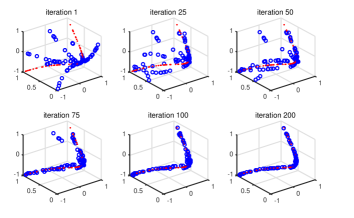
Refer to caption
Figure 6: Recovery result on data drawn from (75) (the red points are the complete data)
Refer to caption
Figure 7: KFMC recovery performance at different iteration on data drawn from (75)

B.2 Compared methods and parameter settings

For offline matrix completion, our KFMC with polynomial kernel and KFMC with RBF kernel are compared with the following methods.

  • LRF (low-rank factorization based matrix completion [27]). LRF is solved by alternating minimization. The matrix rank and regularization parameter are searched within a broad range such that the best results are reported in our experiments.

  • NNM (nuclear norm minimization [4]). NNM is solved by inexact augmented lagrange multiplier [18] and has no parameter to determine beforehand. Therefore it is good baseline for our evaluation.

  • VMC (algebraic variety model for matrix completion [25]). In VMC, second-order polynomial kernel is used, where the hyper-parameter is chosen from {1,10,100}110100\{1,10,100\}. The parameter of Schatten-p𝑝p norm is set as 0.5, which often performs the best. To reduce its computational cost, randomized SVD [12], instead of full SVD, is performed.

  • NLMC (nonlinear matrix completion [10]). In NLMC, RBF kernel is used. The parameter σ𝜎\sigma of the kernel is chosen from {0.5d¯,1d¯,3d¯}0.5¯𝑑1¯𝑑3¯𝑑\{0.5\bar{d},1\bar{d},3\bar{d}\}, where d¯¯𝑑\bar{d} is the average distance of all pair-wise data points. The parameter of Schatten-p𝑝p norm is set as 0.5 and randomized SVD is also performed.

In our KFMC(Poly) method, second order polynomial kernel is used, where the hyper-parameter is set as 1. The regularization parameters α𝛼\alpha and β𝛽\beta are chosen from {0.01,0.1}0.010.1\{0.01,0.1\}. In our KFMC(RBF), the setting of parameter σ𝜎\sigma is the same as that of NLMC. The regularization parameter β𝛽\beta is chosen from {0.001,0.0001}0.0010.0001\{0.001,0.0001\} while α𝛼\alpha does not matter. The parameter r𝑟r of KFMC(Poly) and KFMC(RBF) are chosen from {0.5m,1m,2m}0.5𝑚1𝑚2𝑚\{0.5m,1m,2m\}, where m𝑚m is the row dimension of the matrix.

For online matrix completion, the parameter setting of OL-KFMC is similar to that of KFMC. Our OL-KFMC(Poly) and OL-KFMC(RBF) are compared with the following methods.

  • GROUSE [2]222http://web.eecs.umich.edu/similar-to\simgirasole/?p=110. The learning rate and matrix rank are searched within large ranges to provide the best performances.

  • OL-DLSR (online dictionary learning and sparse representation based matrix completion). OL-DLSR is achieved by integrating [22] with [11]. It solves the following problem

    minimize𝑫𝒞,𝒛12𝝎(𝒙𝑫𝒛)2+λ𝒛1subscriptminimize𝑫𝒞𝒛12superscriptnormdirect-product𝝎𝒙𝑫𝒛2𝜆subscriptnorm𝒛1\mathop{\text{minimize}}_{\bm{D}\in\mathcal{C},\bm{z}}\tfrac{1}{2}\|\bm{\omega}\odot(\bm{x}-\bm{D}\bm{z})\|^{2}+\lambda\|\bm{z}\|_{1} (76)

    for a set of incomplete data columns {𝒙}𝒙\{\bm{x}\}. 𝝎𝝎\bm{\omega} is a binary vector with ωi=0subscript𝜔𝑖0\omega_{i}=0 if entry i𝑖i of 𝒙𝒙\bm{x} is missing and ωi=1subscript𝜔𝑖1\omega_{i}=1 otherwise. According to [11], the method can recover high-rank matrices online when the data are drawn from a union of subspaces. We determine λ𝜆\lambda and the number of columns of 𝑫𝑫\bm{D} carefully to give the best performances of OL-DLSR in our experiments.

  • OL-LRF (online LRF [27, 14]). OL-LRF is similar to OL-DLSR. The only difference is that 𝒛1subscriptnorm𝒛1\|\bm{z}\|_{1} is replaced by 12𝒛F212superscriptsubscriptnorm𝒛𝐹2\dfrac{1}{2}\|\bm{z}\|_{F}^{2}. In OL-LRF, the matrix rank is carefully determined to give the best performances in our experiments.

For out-of-sample extension of matrix completion, our OSE-KFMC is compared with the following two methods.

  • OSE-LRF First, perform SVD on a complete training data matrix, i.e., 𝑿=𝑼𝑺𝑽T𝑿𝑼𝑺superscript𝑽𝑇\bm{X}=\bm{U}\bm{S}\bm{V}^{T}, where 𝑼m×r𝑼superscript𝑚𝑟\bm{U}\in\mathbb{R}^{m\times r}, 𝑺r×r𝑺superscript𝑟𝑟\bm{S}\in\mathbb{R}^{r\times r}, 𝑽n×r𝑽superscript𝑛𝑟\bm{V}\in\mathbb{R}^{n\times r}, and r=rank(𝑿)𝑟rank𝑿r=\text{rank}(\bm{X}). For a new incomplete data column 𝒙𝒙\bm{x}, the missing entries are recovered as

    𝒙ω¯=𝑼ω¯(𝑼ωT𝑼ω+λ𝑰|ω|)1𝑼ωT𝒙ω,subscript𝒙¯𝜔subscript𝑼¯𝜔superscriptsuperscriptsubscript𝑼𝜔𝑇subscript𝑼𝜔𝜆subscript𝑰𝜔1superscriptsubscript𝑼𝜔𝑇subscript𝒙𝜔\bm{x}_{\bar{\omega}}=\bm{U}_{\bar{\omega}}(\bm{U}_{\omega}^{T}\bm{U}_{\omega}+\lambda\bm{I}_{|\omega|})^{-1}\bm{U}_{\omega}^{T}\bm{x}_{\omega}, (77)

    where ω𝜔\omega denotes the locations of observed entries, ω¯¯𝜔\bar{\omega} denotes the locations of missing entries, λ𝜆\lambda is a small constant, and 𝑼ω¯subscript𝑼¯𝜔\bm{U}_{\bar{\omega}} consists of the rows of 𝑼𝑼\bm{U} corresponding to ω¯¯𝜔\bar{\omega}.

  • OSE-DLSR First, a dictionary 𝑫𝑫\bm{D} is learned by the method of [22] from the training data. Given a new incomplete data 𝒙𝒙\bm{x}, we can obtain the sparse coefficient as

    𝒛=min𝒛12𝝎(𝒙𝑫𝒛)2+λ𝒛1.𝒛subscript𝒛12superscriptnormdirect-product𝝎𝒙𝑫𝒛2𝜆subscriptnorm𝒛1\bm{z}=\min\limits_{\bm{z}}\tfrac{1}{2}\|\bm{\omega}\odot(\bm{x}-\bm{D}\bm{z})\|^{2}+\lambda\|\bm{z}\|_{1}. (78)

    Finally, the missing entries of 𝒙𝒙\bm{x} can be recovered as 𝒙ω¯=𝑫ω¯𝒛subscript𝒙¯𝜔subscript𝑫¯𝜔𝒛\bm{x}_{\bar{\omega}}=\bm{D}_{\bar{\omega}}\bm{z}.

The experiments are conducted with MATLAB on a computer with Inter-i7-3.4GHz Core and 16 GB RAM. The maximum iteration of each offline matrix completion method is 500, which is often enough to converge or give a high recovery accuracy. It also provides a baseline to compare the computational costs of VMC, NLMC, and KFMC.

B.3 Synthetic data

Take the case of three nonlinear subspaces as an example, the optimization curves of our KFMC with different momentum parameter η𝜂\eta are shown in Figure 8. We see that a larger η𝜂\eta can lead to a faster convergence. Particularly, compared with KFMC(Poly), KFMC(RBF) requires fewer iterations to converge, while in each iteration the computational cost of the former is a little bit higher than that of the latter. In this paper, we set η=0.5𝜂0.5\eta=0.5 for all experiments.

Refer to caption
Figure 8: Optimization of KFMC with different momentum parameter η𝜂\eta

Figure 9 shows the online KFMC’s iterative changes of empirical cost function

gt(𝑫):=1tj=1t([𝒙j]ωj,𝑫)assignsubscript𝑔𝑡𝑫1𝑡superscriptsubscript𝑗1𝑡subscriptdelimited-[]subscript𝒙𝑗subscript𝜔𝑗𝑫g_{t}(\bm{D}):=\dfrac{1}{t}\sum_{j=1}^{t}\ell([\bm{x}_{j}]_{\omega_{j}},\bm{D}) (79)

and empirical recovery error

et(𝒙):=1tj=1t𝒙j𝒙^j𝒙j,assignsubscript𝑒𝑡𝒙1𝑡superscriptsubscript𝑗1𝑡normsubscript𝒙𝑗subscript^𝒙𝑗normsubscript𝒙𝑗e_{t}(\bm{x}):=\dfrac{1}{t}\sum_{j=1}^{t}\dfrac{\|\bm{x}_{j}-\hat{\bm{x}}_{j}\|}{\|\bm{x}_{j}\|}, (80)

where 𝒙^jsubscript^𝒙𝑗\hat{\bm{x}}_{j} denotes the recovered column and t𝑡t is the number of online samples. At the beginning of the online learning (t𝑡t is small), the recover errors and the values of cost function are high. With the increasing of t𝑡t, the recover errors and the values of cost function decreased. In practice, we can re-pass the data to reduce the recovery errors. In addition, when t𝑡t is large enough and the structure of the data is assumed to be fixed, we do not need to update 𝑫𝑫\bm{D}. If the data structure changes according to time, we can just update 𝑫𝑫\bm{D} all the time in order to adapt to the changes.
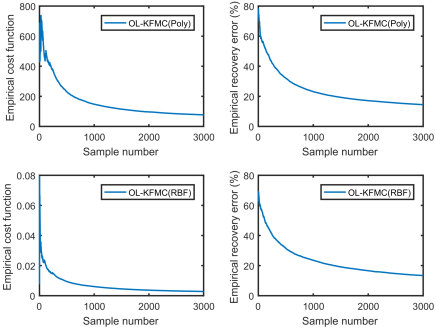
Refer to caption
Figure 9: Empirical cost function and recovery error of online KFMC

In our experiments of online matrix completion, the reported recovery errors are the results after the data matrix was passed for 10 times. Figure 11 shows the matrix completion errors of different number of passes. Our OL-KFMC(Poly) and OL-KFMC(RBF) have the lowest recovery errors. The recovery errors of OL-LRF and GROUSE are considerably high because they are low-rank methods but the matrix in the experiment is of high-rank.
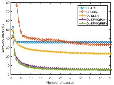
Refer to caption
Figure 10: Matrix completion errors of different passes

B.4 Real data

For the experiments of subspace clustering on incomplete data of Hopkins 155 datasets [28], similar to [25], we conducted the following procedures. First, the two subsets of video sequences, 1R2RC and 1R2TCR, were uniformly downsampled to 6 frames. Then the sizes of the resulted data matrices are 12×4591245912\times 459 and 12×5561255612\times 556. Second, we randomly removed a fraction (10%70%similar-topercent10percent7010\%\sim 70\%) of the entries of the two matrices and then perform matrix completion to recover the missing entries. Finally, SSC (sparse subspace clustering [7]) were performed to segment the data into different clusters. For fair comparison, the parameter λ𝜆\lambda in SSC were chosen from {1,10,100}110100\{1,10,100\} and the best results were reported.

For the CMU motion capture data, similar to [6, 25], we use the trial #6#6\#6 of subject #56#56\#56 of the dataset, which is available at http://mocap.cs.cmu.edu/. The data consists of the following motions: throw punches, grab, skip, yawn, stretch, leap, lift open window, walk, and jump/bound. The data size is 62×678462678462\times 6784. The data of each motion lie in a low-rank subspace and the whole data matrix is of full-rank [6]. To reduce the computational cost and increase the recovery difficulty, we sub-sampled the data to 62×339262339262\times 3392. We considered two types of missing data pattern. The first one is randomly missing, for which we randomly removed 10%percent1010\% to 70%percent7070\% entries of the matrix. The second one is continuously missing, which is more practical and challenging. Specifically, for each row of the matrix, the missing entries were divided into 50 missing sequences, where the sequences are uniformly distributed and the length of each sequence is about 68δ68𝛿68\delta. Here δ𝛿\delta denotes the missing rate. The two missing data patterns are shown in Figure 11, in which the black pixel or region denotes the missing entries. For the online recovery, the number of passes for OL-LRF, GROUSE, OL-DLSR, and OL-KFMC are 10, 50, 10, and 5 respectively. The reason for this setting is that GROUSE requires large number of passes while the other methods especially our OL-KFMC requires fewer passes.
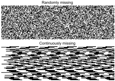
Refer to caption
Figure 11: Two missing data patterns for motion capture data