Familywise Error Rate Control by
Interactive Unmasking

Boyan Duan Aaditya Ramdas Larry Wasserman

{boyand,aramdas,larry}@stat.cmu.edu

Department of Statistics and Data Science,
Carnegie Mellon University, Pittsburgh, PA 15213
Abstract

We propose a method for multiple hypothesis testing with familywise error rate (FWER) control, called the i-FWER test. Most testing methods are predefined algorithms that do not allow modifications after observing the data. However, in practice, analysts tend to choose a promising algorithm after observing the data; unfortunately, this violates the validity of the conclusion. The i-FWER test allows much flexibility: a human (or a computer program acting on the human’s behalf) may adaptively guide the algorithm in a data-dependent manner. We prove that our test controls FWER if the analysts adhere to a particular protocol of “masking” and “unmasking”. We demonstrate via numerical experiments the power of our test under structured non-nulls, and then explore new forms of masking.

1 Introduction

Hypothesis testing is a critical instrument in scientific research to quantify the significance of a discovery. For example, suppose an observation Z𝑍Z\in\mathbb{R} follows a Gaussian distribution with mean μ𝜇\mu and unit variance. We wish to distinguish between the following null and alternative hypotheses regarding the mean value:

H0:μ0versusH1:μ>0.:subscript𝐻0𝜇0versussubscript𝐻1:𝜇0\displaystyle H_{0}:\mu\leq 0\quad\text{versus}\quad H_{1}:\mu>0. (1)

A test decides whether to reject the null hypothesis, usually by calculating a p𝑝p-value: the probability of observing an outcome at least as extreme as the observed data under the null hypothesis. In the above example, the p𝑝p-value is P=1Φ(Z)𝑃1Φ𝑍P=1-\Phi(Z), where ΦΦ\Phi is the cumulative distribution function (CDF) of a standard Gaussian. When the true mean μ𝜇\mu is exactly zero, the p𝑝p-value is uniformly distributed; when μ<0𝜇0\mu<0, it has nondecreasing density. A low p𝑝p-value suggests evidence to reject the null hypothesis.

Recent work on testing focuses on a large number of hypotheses, referred to as multiple testing, driven by various applications in Genome-wide Association Studies, medicine, brain imaging, etc. (see [Farcomeni, 2008; Goeman and Solari, 2014] and references therein). In such a setup, we are given n𝑛n null hypotheses {Hi}i=1nsuperscriptsubscriptsubscript𝐻𝑖𝑖1𝑛\{H_{i}\}_{i=1}^{n} and their p𝑝p-values P1,,Pnsubscript𝑃1subscript𝑃𝑛P_{1},\ldots,P_{n}. A multiple testing method examines the p𝑝p-values, possibly together with some side/prior information, and decides whether to reject each hypothesis (i.e., infers which ones are the non-nulls). Let 0subscript0\mathcal{H}_{0} be the set of hypotheses that are truly null and \mathcal{R} be the set of rejected hypotheses, then V=|0|𝑉subscript0V=|\mathcal{H}_{0}\cap\mathcal{R}| is the number of erroneous rejections. This paper considers a classical error metric, familywise error rate:

FWER:=(V1),assignFWER𝑉1\text{FWER}:=\mathbb{P}(V\geq 1),

which is the probability of making any false rejection. Given a fixed level α(0,1)𝛼01\alpha\in(0,1), a good test should have valid error control that FWER αabsent𝛼\leq\alpha, and high power, defined as the expected proportion of rejected non-nulls:

power:=𝔼(|\0||[n]\0|),assignpower𝔼\subscript0\delimited-[]𝑛subscript0\text{power}:=\mathbb{E}\left(\frac{|\mathcal{R}\backslash\mathcal{H}_{0}|}{|[n]\backslash\mathcal{H}_{0}|}\right),

where [n]:={1,,n}assigndelimited-[]𝑛1𝑛[n]:=\{1,\ldots,n\} denotes the set of all hypotheses.

Most methods with FWER control follow a prespecified algorithm (see, for instance, [Holm, 1979; Hochberg, 1988; Bretz et al., 2009; Goeman and Solari, 2011; Tamhane and Gou, 2018] and references therein). However, in practice, analysts tend to try out several algorithms or parameters on the same dataset until results are “satisfying”. When a second group repeats the same experiments, the outcomes are often not as good. This problem in reproducibility comes from the bias in selecting the analysis tool: researchers choose a promising method after observing the data, which violates the validity of error control. Nonetheless, data would greatly help us understand the problem and choose an appropriate method if it were allowed. This motivates us to propose an interactive method called the i-FWER test, that (a) can use observed data in the design of testing algorithm, and (b) is a multi-step procedure such that a human can monitor the performance of the current algorithm and is allowed to adjust it at any step interactively; and still controls FWER.

p𝑝p-values {Pi}subscript𝑃𝑖\{P_{i}\}{g(Pi)}𝑔subscript𝑃𝑖\{g(P_{i})\}{h(Pi)}subscript𝑃𝑖\{h(P_{i})\}Prior/side information, covariates {xi}subscript𝑥𝑖\{x_{i}\}Rejection set tsubscript𝑡\mathcal{R}_{t}Estimate FWER^tsubscript^FWER𝑡\widehat{\text{FWER}}_{t}Report tsubscript𝑡\mathcal{R}_{t}SelectionError controlMaskingShrinkIf FWER^tαsubscript^FWER𝑡𝛼\widehat{\text{FWER}}_{t}\leq\alphaIf FWER^t>αsubscript^FWER𝑡𝛼\widehat{\text{FWER}}_{t}>\alphaUnmasking
Figure 1: A schematic of the i-FWER test. All p𝑝p-values are initially ‘masked’: all {g(Pi)}𝑔subscript𝑃𝑖\{g(P_{i})\} are revealed to the analyst/algorithm, while all {h(Pi)}subscript𝑃𝑖\{h(P_{i})\} remain hidden, and the initial rejection set is 0=[n]subscript0delimited-[]𝑛\mathcal{R}_{0}=[n]. If FWER^t>αsubscript^FWER𝑡𝛼\widehat{\text{FWER}}_{t}>\alpha, the analyst chooses a p𝑝p-value to ‘unmask’ (observe the masked h(P)𝑃h(P)-value), effectively removing it from the proposed rejection set tsubscript𝑡\mathcal{R}_{t}; importantly, using any available side information and/or covariates and/or working model, the analyst can shrink tsubscript𝑡\mathcal{R}_{t} in any manner. This process continues until FWER^tαsubscript^FWER𝑡𝛼\widehat{\text{FWER}}_{t}\leq\alpha (or t=subscript𝑡\mathcal{R}_{t}=\emptyset).

The word “interactive” is used in many contexts in machine learning and statistics. Specifically, multi-armed bandits, active learning, online learning, reinforcement learning, differential privacy, adaptive data analysis, and post-selection inference all involve some interaction. Each of these paradigms has a different goal, a different model of interaction, and different mathematical tools to enable and overcome the statistical dependencies created by data-dependent interaction. The type of interaction proposed in this paper is different from the above. Here, the goal is to control FWER in multiple testing. The model of interaction involves “masking” of p𝑝p-values followed by progressive unmasking (details in the next paragraph). The technical tools used are (a) for p𝑝p-values of the true nulls (null p𝑝p-values), the masked and revealed information are independent, (b) an empirical upper bound on the FWER that can be continually updated using the revealed information.

The key idea that permits interaction while ensuring FWER control is “masking and unmasking”, proposed by Lei and Fithian [2018]; Lei et al. [2020]. In our method, it has three main steps and alternates between the last two (Figure 1):

  1. 1.

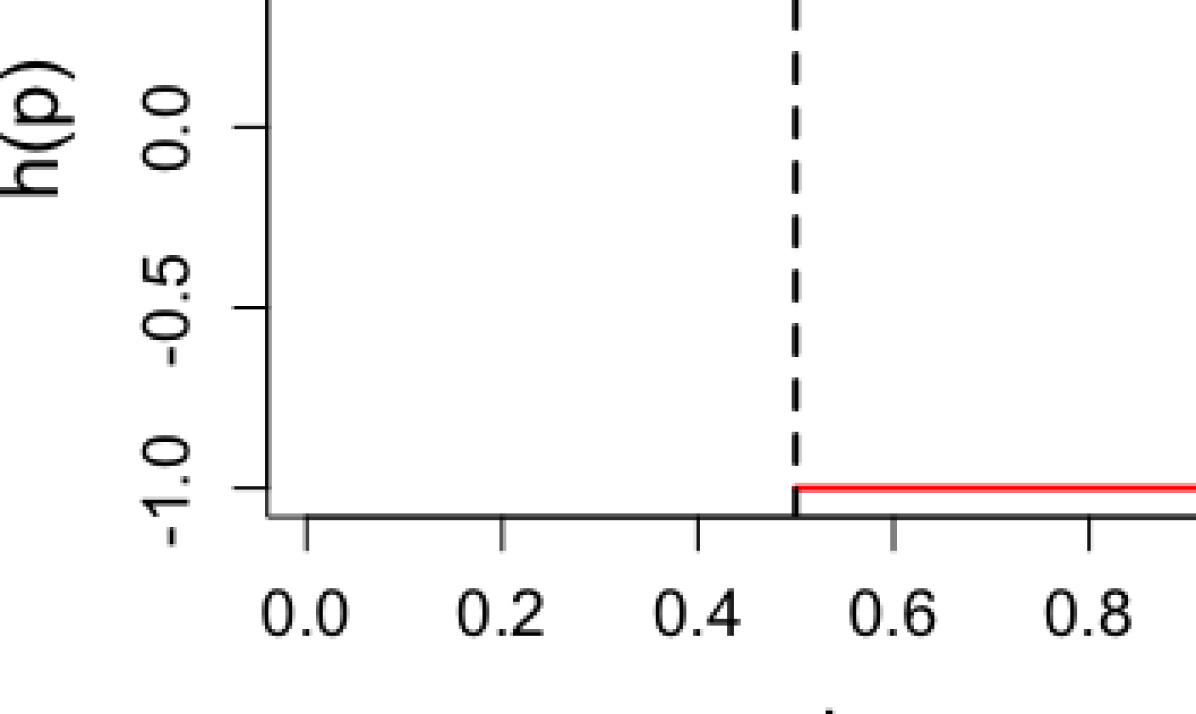
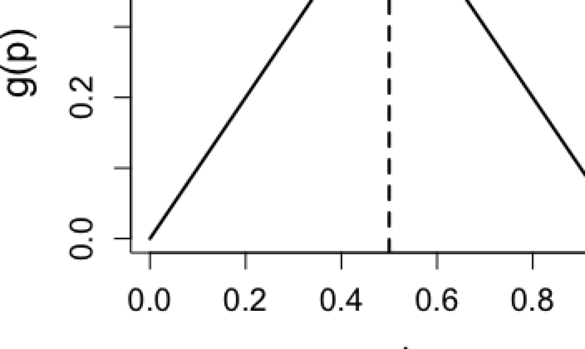
    Masking. Given a parameter p(0,1)subscript𝑝01p_{*}\in(0,1), each p𝑝p-value Pisubscript𝑃𝑖P_{i} is decomposed into two parts by functions h:[0,1]{1,1}:0111h:[0,1]\to\{-1,1\} and g:[0,1](0,p):𝑔010subscript𝑝g:[0,1]\to(0,p_{*}):

    h(Pi;p)=subscript𝑃𝑖subscript𝑝absent\displaystyle h(P_{i};p_{*})=~{} 2𝟙{Pi<p}1;21subscript𝑃𝑖subscript𝑝1\displaystyle 2\cdot\mathbbm{1}\{P_{i}<p_{*}\}-1;{}
    and g(Pi;p)=and 𝑔subscript𝑃𝑖subscript𝑝absent\displaystyle\text{and }g(P_{i};p_{*})=~{} min{Pi,p1p(1Pi)},subscript𝑃𝑖subscript𝑝1subscript𝑝1subscript𝑃𝑖\displaystyle\min\left\{P_{i},\frac{p_{*}}{1-p_{*}}(1-P_{i})\right\}, (2)

    where g(Pi)𝑔subscript𝑃𝑖g(P_{i}), the masked p𝑝p-value, is used to interactively adjust the algorithm, and h(Pi)subscript𝑃𝑖h(P_{i}), the revealed missing bit, is used for error control. Note that h(Pi)subscript𝑃𝑖h(P_{i}) and g(Pi)𝑔subscript𝑃𝑖g(P_{i}) are independent if Hisubscript𝐻𝑖H_{i} is null (Pisubscript𝑃𝑖P_{i} is uniformly distributed); this fact permits interaction with an analyst without any risk of violating FWER control.
    Refer to caption
    Refer to caption
    Figure 2: Functions for masking (1): missing bits hh (left) and masked p𝑝p-values g𝑔g (right) when p=0.5subscript𝑝0.5p_{*}=0.5. For uniform p𝑝p-values, g(P)𝑔𝑃g(P) and h(P)𝑃h(P) are independent.
  2. 2.

    Selection. Consider a set of candidate hypotheses to be rejected (rejection set), denoted as tsubscript𝑡\mathcal{R}_{t} for iteration t𝑡t. We start with all the hypotheses included, 0=[n]subscript0delimited-[]𝑛\mathcal{R}_{0}=[n]. At each iteration, the analyst excludes possible nulls from the previous t1subscript𝑡1\mathcal{R}_{t-1}, using all the available information (masked p𝑝p-values, progressively unmasked h(Pi)subscript𝑃𝑖h(P_{i}) from step 3 and possible prior information). Note that our method does not automatically use prior information and masked p𝑝p-values. The analyst is free to use any black-box prediction algorithm or Bayesian working model that uses the available information, and orders the hypotheses possibly using an estimated likelihood of being non-null. This step is where a human is allowed to incorporate their subjective choices.

  3. 3.

    Error control (and unmasking). The FWER is estimated using h(Pi)subscript𝑃𝑖h(P_{i}). If the estimation FWER^t>αsubscript^FWER𝑡𝛼\widehat{\text{FWER}}_{t}>\alpha, the analyst goes back to step 2, provided with additional information: unmasked (reveal) h(Pi)subscript𝑃𝑖h(P_{i}) of the excluded hypotheses, which improves her understanding of the data and guides her choices in the selection step.

The rest of the paper is organized as follows. In Section 2, we describe the i-FWER test in detail. In Section 3, we implement the interactive test under a clustered non-null structure. In Section 4, we propose two alternative ways of masking p𝑝p-values and explore their advantages.

2 An interactive test with FWER control

Interaction shows its power mostly when there is prior knowledge. We first introduce the side information, which is available before the test in the form of covariates xisubscript𝑥𝑖x_{i} as an arbitrary vector (mix of binary, real-valued, categorical, etc.) for each hypothesis i𝑖i. For example, if the hypotheses are arranged in a rectangular grid (such as when processing an image), then xisubscript𝑥𝑖x_{i} could be the coordinate of hypothesis i𝑖i on the grid. Side information can help the analyst to exclude possible nulls, for example, when the non-nulls are believed to form a cluster on the grid by some domain knowledge. Here, we state the algorithm and error control with the side information treated as fixed values, but side information can be random variables, like the bodyweight of patients when testing whether each patient reacts to a certain medication. Our test also works for random side information Xisubscript𝑋𝑖X_{i} by considering the conditional behavior of p𝑝p-values given Xisubscript𝑋𝑖X_{i}.

The i-FWER test proceeds as progressively shrinking a candidate rejection set tsubscript𝑡\mathcal{R}_{t} at step t𝑡t,

[n]=01n=,delimited-[]𝑛subscript0superset-of-or-equalssubscript1superset-of-or-equalssuperset-of-or-equalssubscript𝑛[n]=\mathcal{R}_{0}\supseteq\mathcal{R}_{1}\supseteq\ldots\supseteq\mathcal{R}_{n}=\emptyset,

where recall [n]delimited-[]𝑛[n] denotes the set of all the hypotheses. We assume without loss of generality that one hypothesis is excluded in each step. Denote the hypothesis excluded at step t𝑡t as itsuperscriptsubscript𝑖𝑡i_{t}^{*}. The choice of itsuperscriptsubscript𝑖𝑡i_{t}^{*} can use the information available to the analyst before step t𝑡t, formally defined as a filtration (sequence of nested σ𝜎\sigma-fields) 111 This filtration denotes the information used for choosing itsuperscriptsubscript𝑖𝑡i_{t}^{*}. The filtration with respect to which the stopping time in Algorithm 1 is measurable includes the scale of Rtsuperscriptsubscript𝑅𝑡R_{t}^{-}: 𝒢t1:=σ(t1,|iRt:h(Pi)=1|){\mathcal{G}_{t-1}:=\sigma\Big{(}\mathcal{F}_{t-1},|i\in R_{t}:h(P_{i})=-1|\Big{)}}.:

t1:=σ({xi,g(Pi)}i=1n,{Pi}it1),assignsubscript𝑡1𝜎superscriptsubscriptsubscript𝑥𝑖𝑔subscript𝑃𝑖𝑖1𝑛subscriptsubscript𝑃𝑖𝑖subscript𝑡1\displaystyle\mathcal{F}_{t-1}:=\sigma\Big{(}\{x_{i},g(P_{i})\}_{i=1}^{n},\{P_{i}\}_{i\notin\mathcal{R}_{t-1}}\Big{)}, (3)

where we unmask the p𝑝p-values for the hypotheses that are excluded from the rejection set t1subscript𝑡1\mathcal{R}_{t-1}.

To control FWER, the number of false discoveries V𝑉V is estimated using only the binary missing bits h(Pi)subscript𝑃𝑖h(P_{i}). The idea is to partition the candidate rejection set tsubscript𝑡\mathcal{R}_{t} into t+superscriptsubscript𝑡\mathcal{R}_{t}^{+} and tsuperscriptsubscript𝑡\mathcal{R}_{t}^{-} by the value of h(Pi)subscript𝑃𝑖h(P_{i}):

t+:=assignsuperscriptsubscript𝑡absent\displaystyle\mathcal{R}_{t}^{+}:=~{} {it:h(Pi)=1}{it:Pi<p},conditional-set𝑖subscript𝑡subscript𝑃𝑖1conditional-set𝑖subscript𝑡subscript𝑃𝑖subscript𝑝\displaystyle\{i\in\mathcal{R}_{t}:h(P_{i})=1\}\equiv\{i\in\mathcal{R}_{t}:P_{i}<p_{*}\},{}
t:=assignsuperscriptsubscript𝑡absent\displaystyle\mathcal{R}_{t}^{-}:=~{} {it:h(Pi)=1}{it:Pip};conditional-set𝑖subscript𝑡subscript𝑃𝑖1conditional-set𝑖subscript𝑡subscript𝑃𝑖subscript𝑝\displaystyle\{i\in\mathcal{R}_{t}:h(P_{i})=-1\}\equiv\{i\in\mathcal{R}_{t}:P_{i}\geq p_{*}\};

recall that psubscript𝑝p_{*} is the prespecified parameter for masking (1). Instead of rejecting every hypothesis in tsubscript𝑡\mathcal{R}_{t}, note that the test only rejects the ones in t+superscriptsubscript𝑡\mathcal{R}_{t}^{+}, whose p𝑝p-values are smaller than psubscript𝑝p_{*} in tsubscript𝑡\mathcal{R}_{t}. Thus, the number of false rejection V𝑉V is |0t+|subscript0superscriptsubscript𝑡{|\mathcal{H}_{0}\cap\mathcal{R}_{t}^{+}|} and we want to control FWER, (V1)𝑉1{\mathbb{P}(V\geq 1)}. The distribution of |0t+|subscript0superscriptsubscript𝑡{|\mathcal{H}_{0}\cap\mathcal{R}_{t}^{+}|} can be estimated by |0t|subscript0superscriptsubscript𝑡|\mathcal{H}_{0}\cap\mathcal{R}_{t}^{-}| using the fact that h(Pi)subscript𝑃𝑖h(P_{i}) is a (biased) coin flip. But 0subscript0\mathcal{H}_{0} (the set of true nulls) is unknown, so we use |t|superscriptsubscript𝑡|\mathcal{R}_{t}^{-}| to upper bound |0t|subscript0superscriptsubscript𝑡|\mathcal{H}_{0}\cap\mathcal{R}_{t}^{-}|, and propose an estimator of FWER:

FWER^t=1(1p)|t|+1.subscript^FWER𝑡1superscript1subscript𝑝superscriptsubscript𝑡1\displaystyle\widehat{\text{FWER}}_{t}=1-(1-p_{*})^{|\mathcal{R}_{t}^{-}|+1}. (4)

Overall, the i-FWER test shrinks tsubscript𝑡\mathcal{R}_{t} until FWER^tαsubscript^FWER𝑡𝛼\widehat{\text{FWER}}_{t}\leq\alpha and rejects only the hypotheses in t+superscriptsubscript𝑡\mathcal{R}_{t}^{+} (Algorithm 1).

Algorithm 1 The i-FWER test
  Input: Side information and p𝑝p-values {xi,Pi}i=1nsuperscriptsubscriptsubscript𝑥𝑖subscript𝑃𝑖𝑖1𝑛\{x_{i},P_{i}\}_{i=1}^{n}, target FWER level α𝛼\alpha, and parameter psubscript𝑝p_{*};
  Procedure:
  Initialize 0=[n]subscript0delimited-[]𝑛\mathcal{R}_{0}=[n];
  for t=1𝑡1t=1 to n𝑛n do
     1. Pick any itt1superscriptsubscript𝑖𝑡subscript𝑡1i_{t}^{*}\in\mathcal{R}_{t-1}, using {xi,g(Pi)}i=1nsuperscriptsubscriptsubscript𝑥𝑖𝑔subscript𝑃𝑖𝑖1𝑛\{x_{i},g(P_{i})\}_{i=1}^{n} and progressively unmasked {h(Pi)}it1subscriptsubscript𝑃𝑖𝑖subscript𝑡1\{h(P_{i})\}_{i\notin\mathcal{R}_{t-1}};
     2. Exclude itsuperscriptsubscript𝑖𝑡i_{t}^{*} and update t=t1\{it}subscript𝑡\subscript𝑡1superscriptsubscript𝑖𝑡{\mathcal{R}_{t}=\mathcal{R}_{t-1}\backslash\{i_{t}^{*}\}};
     if FWER^t1(1p)|t|+1αsubscript^FWER𝑡1superscript1subscript𝑝superscriptsubscript𝑡1𝛼\widehat{\text{FWER}}_{t}\equiv 1-(1-p_{*})^{|\mathcal{R}_{t}^{-}|+1}\leq\alpha then
        Reject {Hi:it,h(Pi)=1}conditional-setsubscript𝐻𝑖formulae-sequence𝑖subscript𝑡subscript𝑃𝑖1\{H_{i}:i\in\mathcal{R}_{t},h(P_{i})=1\} and exit;
     end if
  end for
Remark 1.

The parameter psubscript𝑝p_{*} should be chosen in (0,α]0𝛼(0,\alpha], because otherwise FWER^tsubscript^FWER𝑡\widehat{\text{FWER}}_{t} is always larger than α𝛼\alpha and no rejection would be made. In principle, because |t|superscriptsubscript𝑡|\mathcal{R}_{t}^{-}| only takes integer values, we should psubscript𝑝p_{*} such that log(1α)log(1p)1𝛼1subscript𝑝\frac{\log(1-\alpha)}{\log(1-p_{*})} is an integer; otherwise, the estimated FWER at the stopping time, FWER^τsubscript^FWER𝜏\widehat{\text{FWER}}_{\tau}, would be strictly smaller than α𝛼\alpha rather than equal. Our numerical experiments suggest that the power is relatively robust to the choice of psubscript𝑝p_{*}. A default choice can be pα/2subscript𝑝𝛼2p_{*}\approx\alpha/2 (see detailed discussion in Appendix G).

Remark 2.

The above procedure can be easily extended to control k𝑘k-FWER:

k-FWER:=(Vk),assign𝑘-FWER𝑉𝑘\displaystyle k\text{-FWER}:=\mathbb{P}(V\geq k), (5)

by estimating k𝑘k-FWER as

k-FWER^t=1i=0k1(|t|+ii)(1p)|t|+1pi.subscript^𝑘-FWER𝑡1superscriptsubscript𝑖0𝑘1binomialsuperscriptsubscript𝑡𝑖𝑖superscript1subscript𝑝superscriptsubscript𝑡1superscriptsubscript𝑝𝑖\displaystyle\widehat{k\text{-FWER}}_{t}=1-\sum_{i=0}^{k-1}\binom{|\mathcal{R}_{t}^{-}|+i}{i}(1-p_{*})^{|\mathcal{R}_{t}^{-}|+1}p_{*}^{i}.

The error control of i-FWER test uses an observation that at the stopping time, the number of false rejections is stochastically dominated by a negative binomial distribution. The complete proof is in Appendix B.

Theorem 1.

Suppose the null p𝑝p-values are mutually independent and they are independent of the non-nulls, then the i-FWER test controls FWER at level α𝛼\alpha.

Remark 3.

The null p𝑝p-values need not be exactly uniformly distributed. For example, FWER control also holds when the null p𝑝p-values have nondecreasing densities. Appendix A presents the detailed technical condition for the distribution of the null p𝑝p-values.

Related work.

The i-FWER test mainly combines and generalizes two sets of work: (a) we use the idea of masking from Lei and Fithian [2018]; Lei et al. [2020] and extend it to a more stringent error metric, FWER; (b) we use the method of controlling FWER from Janson and Su [2016] by converting a one-step procedure in the context of “knockoff” statistics in regression problem to a multi-step (interactive) procedure in our context of p𝑝p-values.

Lei and Fithian [2018] and Lei et al. [2020] introduce the idea of masking and propose interactive tests that control false discovery rate (FDR):

FDR:=𝔼(V||1),assignFDR𝔼𝑉1\text{FDR}:=\mathbb{E}\left(\frac{V}{|\mathcal{R}|\vee 1}\right),

the expected proportion of false discoveries. It is less stringent than FWER, the probability of making any false discovery. Their method uses the special case of masking (1) when p=0.5subscript𝑝0.5p_{*}=0.5, and estimate V𝑉V by it𝟙{h(Pi)=1}subscript𝑖subscript𝑡1subscript𝑃𝑖1\sum_{i\in\mathcal{R}_{t}}\mathbbm{1}\{h(P_{i})=-1\}, or equivalently it𝟙{Pi<0.5}subscript𝑖subscript𝑡1subscript𝑃𝑖0.5\sum_{i\in\mathcal{R}_{t}}\mathbbm{1}\{P_{i}<0.5\}. While it provides a good estimation on the proportion of false discoveries, the indicator 𝟙{Pi<0.5}1subscript𝑃𝑖0.5\mathbbm{1}\{P_{i}<0.5\} has little information on the correctness of individual rejections. To see this, suppose there is one rejection, then FWER is the probability of this rejection being false. Even if h(Pi)=1subscript𝑃𝑖1h(P_{i})=1, which indicates the p𝑝p-value is on the smaller side, the tightest upper bound on FWER is as high as 0.50.50.5. Thus, our method uses masking (1) with small psubscript𝑝p_{*}, so that h(Pi)=1subscript𝑃𝑖1h(P_{i})=1, or equivalently Pi<psubscript𝑃𝑖subscript𝑝P_{i}<p_{*}, suggests a low chance of false rejection.

In the context of a regression problem to select significant covariates, Janson and Su [2016] proposes a one-step method with control on k𝑘k-FWER; recall definition in (5). The FWER is a special case of k𝑘k-FWER when k=1𝑘1k=1, and as k𝑘k grows larger, k𝑘k-FWER is a less stringent error metric. Their method decomposes statistics called “knockoff” [Barber and Candès, 2015] into the magnitudes for ordering covariates (without interaction) and signs for estimating k𝑘k-FWER, which corresponds to decomposing p𝑝p-values into g(Pi)𝑔subscript𝑃𝑖g(P_{i}) and h(Pi)subscript𝑃𝑖h(P_{i}) when p=0.5subscript𝑝0.5p_{*}=0.5. However, the decomposition as magnitude and sign restricts the corresponding p𝑝p-value decomposition with a single choice of psubscript𝑝p_{*} as 0.50.50.5, making the k𝑘k-FWER control conservative and power low when k=1𝑘1k=1; yet our method shows high power in experiments. Their error control uses the connection between k𝑘k-FWER and a negative binomial distribution, based on which we propose the estimator FWER^tsubscript^FWER𝑡\widehat{\text{FWER}}_{t} for our multi-step procedure, and prove the error control even when interaction is allowed. As far as we know, this estimator viewpoint of the FWER procedure is also new in the literature.

Jelle Goeman (private communication) pointed out that the i-FWER test can be interpreted from the perspective of closed testing [Marcus et al., 1976]. Our method is also connected with the fallback procedure [Wiens and Dmitrienko, 2005], which allows for arbitrary dependence but is not interactive and combine covariate information with p𝑝p-values to determine the ordering. See Appendix C for details.

The i-FWER test in practice.

Technically in a fully interactive procedure, a human can examine all the information in t1subscript𝑡1\mathcal{F}_{t-1} and pick itsuperscriptsubscript𝑖𝑡i_{t}^{*} subjectively or by any other principle, but doing so for every step could be tedious and unnecessary. Instead, the analyst can design an automated version of the i-FWER test, and still keeps the flexibility to change it at any iteration. For example, the analyst can implement an automated algorithm to first exclude 80%percent8080\% hypotheses (say). If FWER^tsubscript^FWER𝑡\widehat{\text{FWER}}_{t} is still larger than level α𝛼\alpha, the analyst can pause the procedure manually to look at the unmasked p𝑝p-value information, update her prior knowledge, and modify the current algorithm. The next section presents an automated implementation of the i-FWER test that takes into account the structure on the non-nulls.

3 An instantiation of an automated algorithm, and numerical experiments

One main advantage of the i-FWER test is the flexibility to include prior knowledge and human guidance. The analyst might have an intuition about what structural constraints the non-nulls have. For example, we consider two structures: (a) a grid of hypotheses where the non-nulls are in a cluster (of some size/shape, at some location; see Figure 3(a)), which is a reasonable prior belief when one wants to identify a tumor in a brain image; and (b) a tree of hypotheses where a child can be non-null only if its parent is non-null, as may be the case in applications involving wavelet decompositions.

Refer to caption
(a) True non-nulls (21 hypotheses).
Refer to caption
(b) 18 rejections by the i-FWER test.
Refer to caption
(c) 7 rejections by the Šidák correction
Figure 3: An instance of rejections by the i-FWER test and the Šidák correction [Šidák, 1967]. Clustered non-nulls are simulated from the setting in Section Setting with a fixed alternative mean μ=3𝜇3\mu=3.

3.1 An example of an automated algorithm under clustered non-null structure

We propose an automated algorithm of the i-FWER test that incorporates the structure of clustered non-nulls. Here, the side information xisubscript𝑥𝑖x_{i} is the coordinates of each hypothesis i𝑖i. The idea is that at each step of excluding possible nulls, we peel off the boundary of the current tsubscript𝑡\mathcal{R}_{t}, such that the rejection set stays connected (see Figure 4).

Refer to caption
Refer to caption
Refer to caption
Refer to caption
Figure 4: An illustration of tsubscript𝑡\mathcal{R}_{t} generated by the automated algorithm described in Section 3.1, at t=50,100,150𝑡50100150t=50,100,150 and t=220𝑡220t=220 when the algorithm stops. The p𝑝p-values in tsubscript𝑡\mathcal{R}_{t} are plotted.

Suppose each hypothesis Hisubscript𝐻𝑖H_{i} has a score Sisubscript𝑆𝑖S_{i} to measure the likelihood of being non-null (non-null likelihood). A simple example is Si=g(Pi)subscript𝑆𝑖𝑔subscript𝑃𝑖S_{i}=-g(P_{i}) since larger g(Pi)𝑔subscript𝑃𝑖g(P_{i}) indicates less chance of being a non-null (more details on Sisubscript𝑆𝑖S_{i} to follow). We now describe an explicit fixed procedure to shrink tsubscript𝑡\mathcal{R}_{t}. Given two parameters d𝑑d and δ𝛿\delta (eg. d=5,δ=5%formulae-sequence𝑑5𝛿percent5d=5,\delta=5\%), it replaces step 1 and 2 in Algorithm 1 as follows:

  1. (a)

    Divide t1subscript𝑡1\mathcal{R}_{t-1} from its center to d𝑑d cones (like slicing a pizza); in each cone, consider a fraction δ𝛿\delta of hypotheses farthest from the center, denoted t11,,t1dsuperscriptsubscript𝑡11superscriptsubscript𝑡1𝑑\smash{\mathcal{R}_{t-1}^{1},\ldots,\mathcal{R}_{t-1}^{d}};

  2. (b)

    Compute S¯j=1|t1j|it1jSisuperscript¯𝑆𝑗1superscriptsubscript𝑡1𝑗subscript𝑖superscriptsubscript𝑡1𝑗subscript𝑆𝑖{\bar{S}^{j}=\frac{1}{|\mathcal{R}_{t-1}^{j}|}\sum_{i\in\mathcal{R}_{t-1}^{j}}S_{i}} for j=1,,d𝑗1𝑑j=1,\ldots,d;

  3. (c)

    Update t=t1\t1ksubscript𝑡\subscript𝑡1superscriptsubscript𝑡1𝑘{\mathcal{R}_{t}=\mathcal{R}_{t-1}\backslash\mathcal{R}_{t-1}^{k}}, where k=argminjS¯j𝑘subscriptargmin𝑗superscript¯𝑆𝑗{k=\operatorname*{argmin}_{j}\bar{S}^{j}}.

The score Sisubscript𝑆𝑖S_{i} that estimates the non-null likelihood can be computed with the aid of a working statistical model. For example, consider a mixture model where each p𝑝p-value Pisubscript𝑃𝑖P_{i} is drawn from a mixture of a null distribution F0subscript𝐹0F_{0} (eg: uniform) with probability 1πi1subscript𝜋𝑖1-\pi_{i} and an alternative distribution F1subscript𝐹1F_{1} (eg: beta distribution) with probability πisubscript𝜋𝑖\pi_{i}, or equivalently,

Pi=𝑑(1πi)F0+πiF1.subscript𝑃𝑖𝑑1subscript𝜋𝑖subscript𝐹0subscript𝜋𝑖subscript𝐹1\displaystyle P_{i}\overset{d}{=}(1-\pi_{i})F_{0}+\pi_{i}F_{1}. (6)

To account for the clustered structure of non-nulls, we may further assume a model that treats πisubscript𝜋𝑖\pi_{i} as a smooth function of the covariates xisubscript𝑥𝑖x_{i}. The hidden missing bits {h(Pi)}iRtsubscriptsubscript𝑃𝑖𝑖subscript𝑅𝑡\{h(P_{i})\}_{i\in R_{t}} can be inferred from g(Pi)𝑔subscript𝑃𝑖g(P_{i}) and the unmasked h(Pi)subscript𝑃𝑖h(P_{i}) by the EM algorithm (see details in Appendix H). As Rtsubscript𝑅𝑡R_{t} shrinks, progressively unmasked missing bits improve the estimation of non-null likelihood and increase the power. Importantly, the FWER is controlled regardless of the correctness of the above model or any other heuristics to shrink Rtsubscript𝑅𝑡R_{t}.

The above algorithm is only one automated example and there are many possibilities of what we can do to shrink Rtsubscript𝑅𝑡R_{t}.

  1. 1.

    A different algorithm can be developed for a different structure. For example, when hypotheses have a hierarchical structure and the non-nulls only appear on a subtree, an algorithm can gradually cut branches.

  2. 2.

    The score Sisubscript𝑆𝑖S_{i} for non-null likelihood is not exclusive for the above algorithm – it can be used in any heuristics such as directly ordering hypotheses by Sisubscript𝑆𝑖S_{i}.

  3. 3.

    Human interaction can help the automated procedure: the analyst can stop and modify the automated algorithm at any iteration. It is a common case where prior knowledge might not be accurate, or there exist several plausible structures. The analyst may try different algorithms and improve their understanding of the data as the test proceeds. In the example of clustered non-nulls, the underlying truth might have two clustered non-nulls instead of one. After several iterations of the above algorithm that is designed for a single cluster, the shape of tsubscript𝑡\mathcal{R}_{t} could look like a dumbbell, so the analyst can split tsubscript𝑡\mathcal{R}_{t} into two subsets if they wish.

Note that there is no universally most powerful test in nonparametric settings since we do not make assumptions on the distribution of non-null p𝑝p-values, or how informative the covariates are. It is possible that the classical Bonferroni-Holm procedure [Holm, 1979] might have high power if applied with appropriate weights. Likewise, the power of our own test might be improved by changing the working model or choosing some other heuristic to shrink tsubscript𝑡\mathcal{R}_{t}. The main advantage of our method is that it can accommodate structural and covariate information and revise the modeling on the fly (as p𝑝p-values are unmasked) while other methods commit to one type of structure without looking at the data.

Next, we demonstrate via experiments that the i-FWER test can improve power over the Šidák correction, a baseline method that does not take side information into account222In all experiments, the Hommel method has similar power to the Šidák correction, and was hence omitted.. We chose a clustered non-null structure for visualization and intuition, though our test can utilize any covariates, structural constraints, domain knowledge, etc.

3.2 Numerical experiments for clustered non-nulls

For most simulations in this paper, we use the setting below,

Setting.

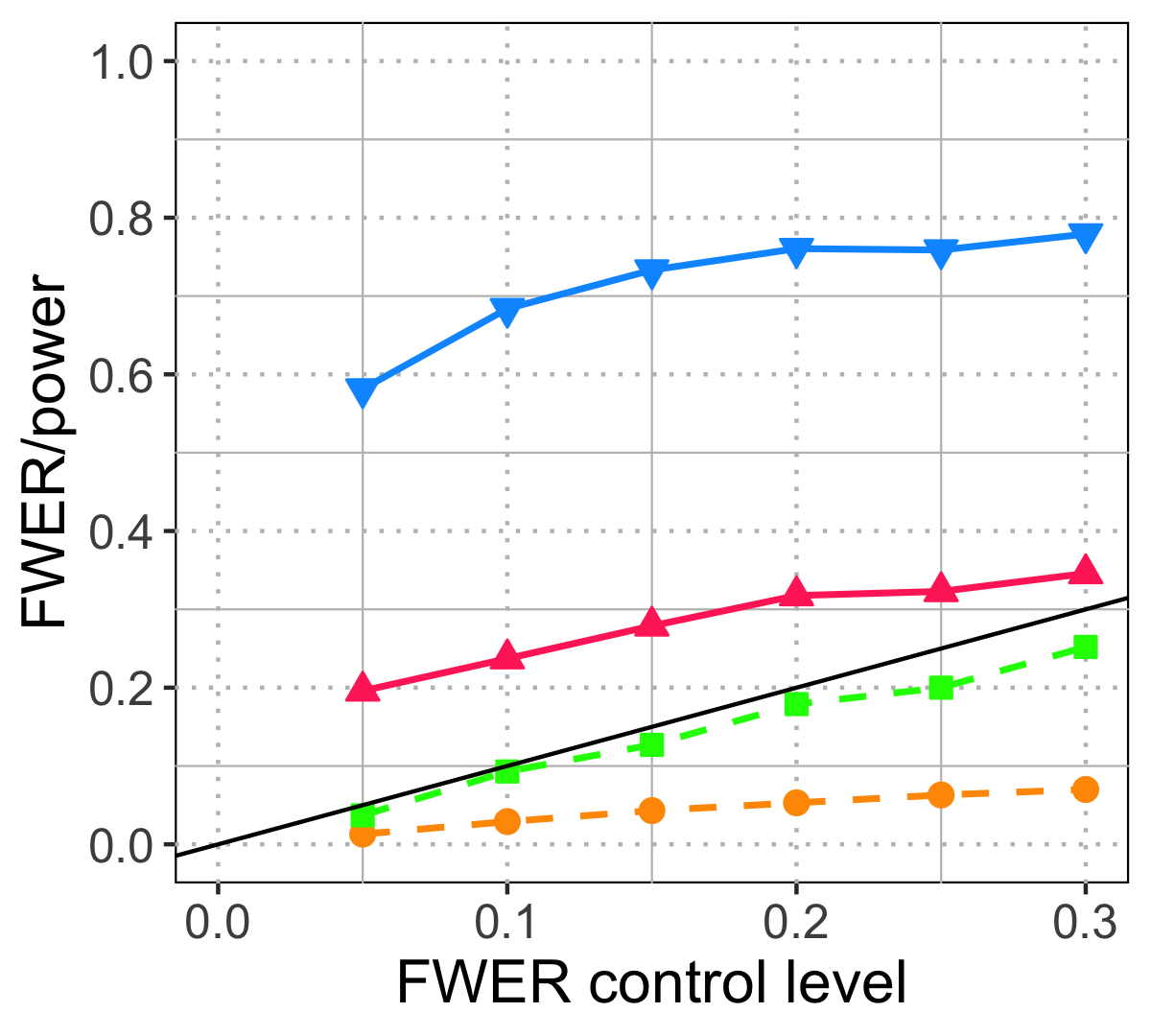
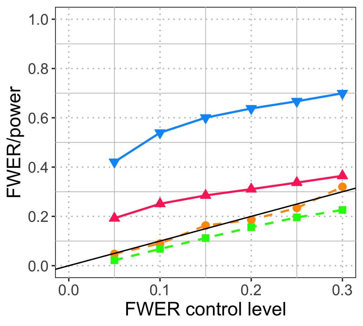
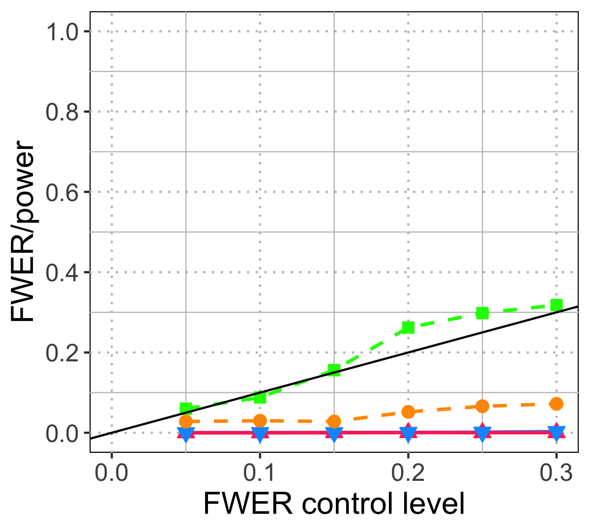
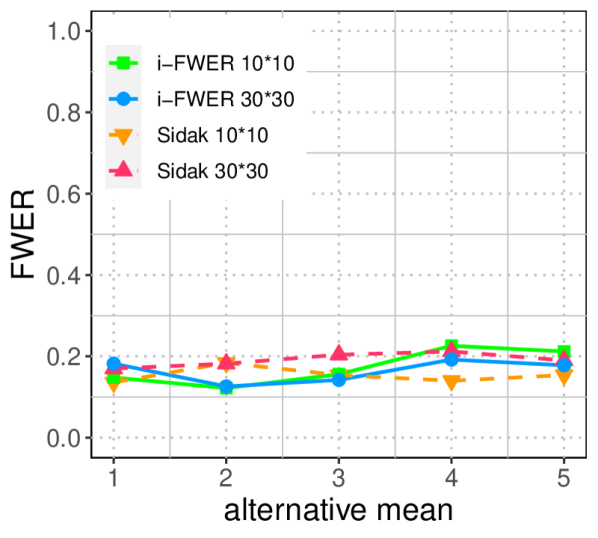
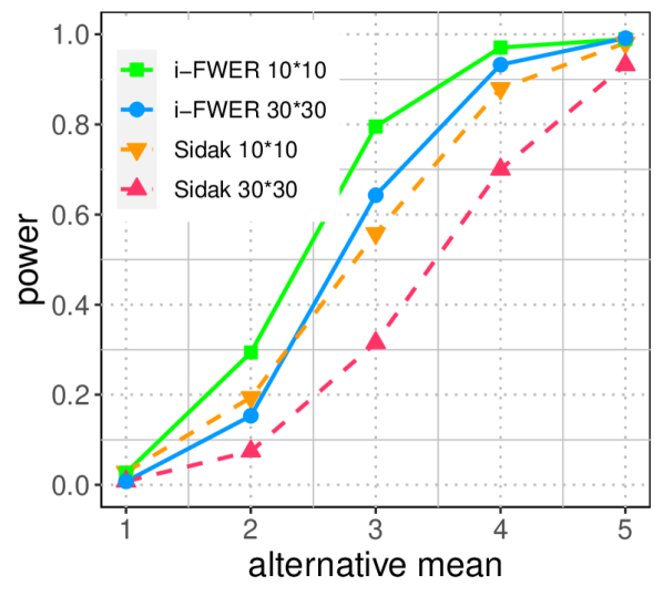
Consider 900 hypotheses arranged in a 30×30303030\times 30 grid with a disc of 21 non-nulls. Each hypothesis tests the mean value of a univariate Gaussian as described in (1). The true nulls are generated from N(0,1)𝑁01N(0,1) and non-nulls from N(μ,1)𝑁𝜇1N(\mu,1), where we varied μ𝜇\mu as (1,2,3,4,5)12345(1,2,3,4,5). For all experiments in the paper, the FWER control is set at level α=0.2𝛼0.2\alpha=0.2, and the power is averaged over 500 repetitions333The standard error of FWER and averaged power are less than 0.02, thus ignored from the plots in this paper..
Refer to caption
Refer to caption
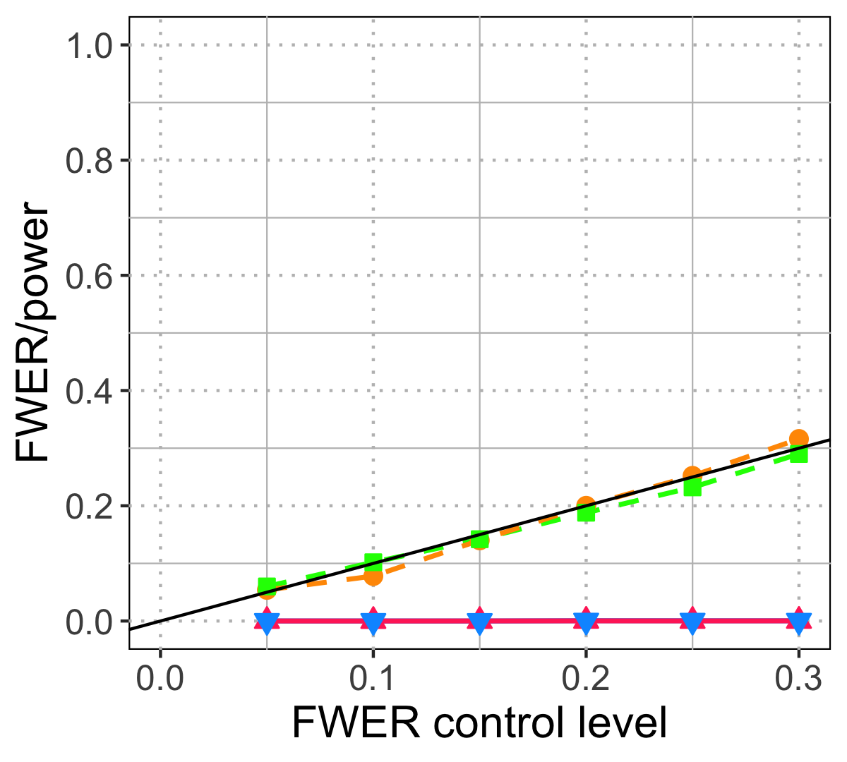
Figure 5: The i-FWER test versus Šidák for clustered non-nulls. The experiments are described in Section Setting where we tried two sizes of hypotheses grid: 10×10101010\times 10 and 30×30303030\times 30 (the latter is a harder problem since the number of nulls increases while the number of non-nulls remains fixed). Both methods show valid FWER control (left). The i-FWER test has higher power under both grid sizes (right).

The i-FWER test has higher power than the Šidák correction, which does not use the non-null structure (see Figure 5). It is hard for most existing methods to incorporate the knowledge that non-nulls are clustered without knowing the position or the size of this cluster. By contrast, such information can be learned in the i-FWER test by looking at the masked p𝑝p-values and the progressively unmasked missing bits. This advantage of the i-FWER test is more evident as the number of nulls increases (by increasing the grid size from 10×101010{10\times 10} to 30×30303030\times 30 with the number of non-nulls fixed). Note that the power of both methods decreases, but the i-FWER test seems less sensitive. This robustness to nulls is expected as the i-FWER test excludes most nulls before rejection, whereas the Šidák correction treats all hypotheses equally.

3.3 An example of an automated algorithm under a hierarchical structure of hypotheses

When the hypotheses form a tree, the side information xisubscript𝑥𝑖x_{i} encodes the parent-child relationship (the set of indices of the children nodes for each hypothesis i𝑖i). Suppose we have prior knowledge that a node cannot be non-null if its parent is null, meaning that the non-nulls form a subtree with the same root. We now develop an automated algorithm that prunes possible nulls among the leaf nodes of current tsubscript𝑡\mathcal{R}_{t}, such that the rejection set has such a subtree shape. Like the algorithm for clustered non-nulls, we use a score Sisubscript𝑆𝑖S_{i} to choose which leaf nodes to exclude. For example, the score Sisubscript𝑆𝑖S_{i} can be the estimated non-null likelihood learned from model (6), where we account for the hierarchical structure by further assuming a partial order constraint on πisubscript𝜋𝑖\pi_{i} that πiπjsubscript𝜋𝑖subscript𝜋𝑗\pi_{i}\geq\pi_{j} if jxi𝑗subscript𝑥𝑖j\in x_{i} (i.e., i𝑖i is the parent of j𝑗j).

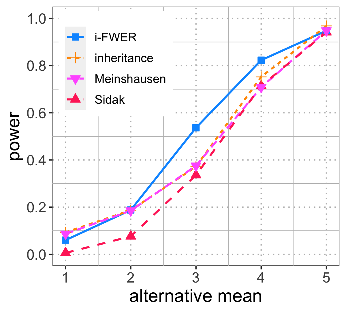
We simulate a tree of five levels (the root has twenty children and three children for each parent node after that) with 801 nodes in total and 7 of them being non-nulls. The non-nulls gather in one of the twenty subtrees of the root. Individual p𝑝p-values are generated by the hypotheses of testing zero-mean Gaussian, same as for the clustered structure, where we varied the non-null mean values μ𝜇\mu as (1,2,3,4,5)12345(1,2,3,4,5).

Refer to caption
Figure 6: Power of the i-FWER test under a tree structure when varying the alternative mean value. It has higher power than inheritance procedure, Meinshausen’s method, and the Sidak correction.

In addition to the Šidák correction, we compare the i-FWER test with two other methods for tree-structured hypotheses: Meinshausen’s method [Meinshausen, 2008] and the inheritance procedure [Goeman and Finos, 2012], which work under arbitrary dependence. Their idea is to pass the error budget from a parent node to its children in a prefixed manner, whereas our algorithm picks out the subtree with non-nulls based on the observed data. In our experiments, the i-FWER test has the highest power (see Figure 6).

The above results demonstrate the power of the i-FWER test in one particular form where the masking is defined as (1). However, any two functions that decompose the null p𝑝p-values into two independent parts can, in fact, be used for masking and fit into the framework of the i-FWER test (see the proofs of error control when using the following new masking functions in Appendix F). In the next section, we explore several choices of masking.

4 New masking functions

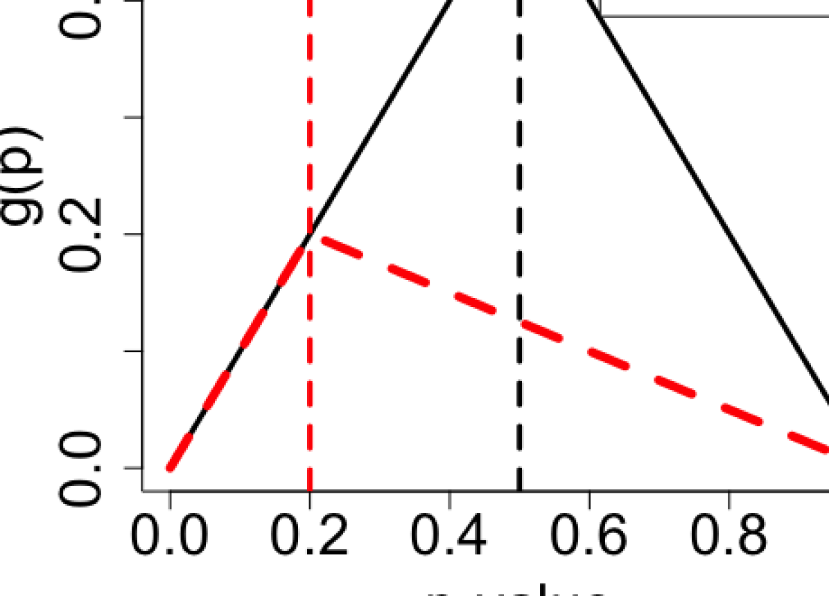
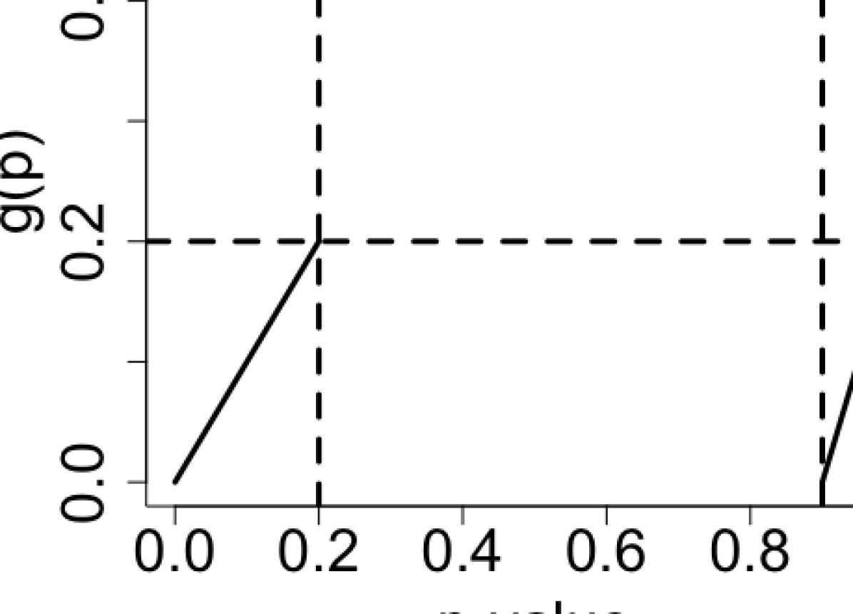
Recall that masking is the key idea that permits interaction and controls error at the same time, by decomposing the p𝑝p-values into two parts: masked p𝑝p-value g(P)𝑔𝑃g(P) and missing bits h(P)𝑃h(P). Such splitting distributes the p𝑝p-value information for two different purposes, interaction and error control, leading to a tradeoff. More information in g(P)𝑔𝑃g(P) provides better guidance on how to shrink tsubscript𝑡\mathcal{R}_{t} and improves the power, while more information in h(P)𝑃h(P) enhances the accuracy of estimating FWER and makes the test less conservative. This section explores several ways of masking and their influence on the power of the i-FWER test. To distinguish different masking functions, we refer to masking (1) introduced at the very beginning as the “tent” function based on the shape of map g𝑔g (see Figure 7(a)).

Refer to caption
(a) Tent functions when psubscript𝑝p_{*} varies as (0.5,0.2)0.50.2(0.5,0.2). We need pαsubscript𝑝𝛼p_{*}\leq\alpha for FWER control.
Refer to caption
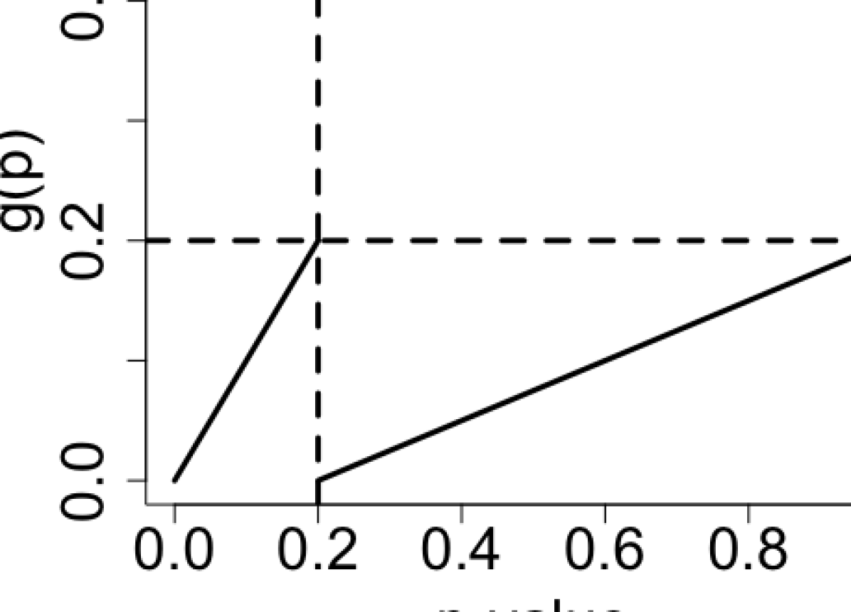
(b) The railway function when p=0.2subscript𝑝0.2p_{*}=0.2.
Refer to caption
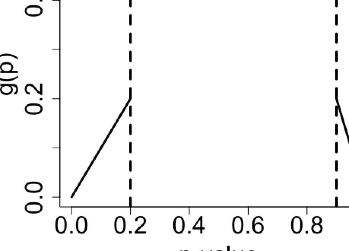
(c) The gap function when (pl,pu)=(0.2,0.9)subscript𝑝𝑙subscript𝑝𝑢0.20.9{(p_{l},p_{u})=(0.2,0.9)}.
Refer to caption
(d) The gap-railway function when (pl,pu)=(0.2,0.9)subscript𝑝𝑙subscript𝑝𝑢0.20.9{(p_{l},p_{u})=(0.2,0.9)}.
Figure 7: Different masking functions leaves different amount of information to g(P)𝑔𝑃g(P) (and the complement part to h(P)𝑃h(P)).

4.1 The “railway” function

We start with an adjustment to the tent function that flips the map g𝑔g when p>p𝑝subscript𝑝p>p_{*}, which we call the “railway” function (see Figure 7(b)). It does not change the information distribution between g(P)𝑔𝑃g(P) and h(P)𝑃h(P), and yet improves the power when nulls are conservative, as demonstrated later. Conservative nulls are often discussed under a general form of hypotheses testing for a parameter θ𝜃\theta:

H0:θΘ0versusH1:θΘ1,:subscript𝐻0𝜃subscriptΘ0versussubscript𝐻1:𝜃subscriptΘ1H_{0}:\theta\in\Theta_{0}\quad\text{versus}\quad H_{1}:\theta\in\Theta_{1},

where Θ0subscriptΘ0\Theta_{0} and Θ1subscriptΘ1\Theta_{1} are two disjoint sets. Conservative nulls are those whose true parameter θ𝜃\theta lies in the interior of Θ0subscriptΘ0\Theta_{0}. For example, when testing whether a Gaussian N(μ,1)𝑁𝜇1N(\mu,1) has nonnegative mean in (1) where Θ0={μ0}subscriptΘ0𝜇0\Theta_{0}=\{\mu\leq 0\}, the nulls are conservative when μ<0𝜇0\mu<0. The resulting p𝑝p-values are biased toward larger values, which compared to the uniform p𝑝p-values from nonconservative nulls should be easier to distinguish from that of non-nulls. However, most classical methods do not take advantage of it, but the i-FWER test can, when using the railway function for masking:

h(Pi)=subscript𝑃𝑖absent\displaystyle h(P_{i})=~{} 2𝟙{Pi<p}1;21subscript𝑃𝑖subscript𝑝1\displaystyle 2\cdot\mathbbm{1}\{P_{i}<p_{*}\}-1;{}
and g(Pi)=and 𝑔subscript𝑃𝑖absent\displaystyle\text{and }g(P_{i})=~{} {Pi,0Pi<p,p1p(Pip),pPi1.casessubscript𝑃𝑖0subscript𝑃𝑖subscript𝑝subscript𝑝1subscript𝑝subscript𝑃𝑖subscript𝑝subscript𝑝subscript𝑃𝑖1\displaystyle\begin{cases}P_{i},&0\leq P_{i}<p_{*},\\ \frac{p_{*}}{1-p_{*}}(P_{i}-p_{*}),&p_{*}\leq P_{i}\leq 1.\end{cases} (7)

The above masked p𝑝p-value, compared with the tent masking (1), can better distinguish the non-nulls from the conservative nulls. To see this, consider a p𝑝p-value of 0.99. When p=0.2subscript𝑝0.2p_{*}=0.2, the masked p𝑝p-value generated by the originally proposed tent function would be 0.0025, thus causing potential confusion with a non-null, whose masked p𝑝p-value is also small. But the masked p𝑝p-value from the railway function would be 0.1975, which is close to 0.20.20.2, the upper bound of g(Pi)𝑔subscript𝑃𝑖g(P_{i}). Thus, it can easily be excluded by our algorithm.

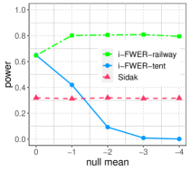
We follow the setting in Section Setting for simulation , except that the alternative mean is fixed as μ=3𝜇3\mu=3, and the nulls are simulated from N(μ0,1)𝑁subscript𝜇01N(\mu_{0},1), where the mean value μ0subscript𝜇0\mu_{0} is negative so that the resulting null p𝑝p-values are conservative. We tried μ0subscript𝜇0\mu_{0} as (0,1,2,3,4)01234(0,-1,-2,-3,-4), with a smaller value indicating higher conservativeness, in the sense that the p𝑝p-values are more likely to be biased to a larger value. When the null is not conservative (μ0=0subscript𝜇00\mu_{0}=0), the i-FWER test with the railway function and tent function have similar power. As the conservativeness of nulls increases, while the power of the i-FWER test with the tent function decreases and the Šidák correction stays the same, the power of the i-FWER test with the railway function increases (see Figure 8).
Refer to caption
Figure 8: Power of the i-FWER test with the tent function and the railway function, where the nulls become more conservative as the null mean decreases in (0,1,2,3,4)01234(0,-1,-2,-3,-4). The i-FWER test benefits from conservative null when using the railway function.

4.2 The “gap” function

Another form of masking we consider maps only the p𝑝p-values that are close to 00 or 111, which is referred to as the “gap” function (see Figure 7(c)) . The resulting i-FWER test directly unmasks all the p𝑝p-values in the middle, and as a price, never rejects the corresponding hypotheses. Given two parameters plsubscript𝑝𝑙p_{l} and pusubscript𝑝𝑢p_{u}, the gap function is defined as

h(Pi)=subscript𝑃𝑖absent\displaystyle h(P_{i})=~{} {1,0Pi<pl,1,pu<Pi1;cases10subscript𝑃𝑖subscript𝑝𝑙1subscript𝑝𝑢subscript𝑃𝑖1\displaystyle\begin{cases}1,&0\leq P_{i}<p_{l},\\ -1,&p_{u}<P_{i}\leq 1;\end{cases}{}
and g(Pi)=and 𝑔subscript𝑃𝑖absent\displaystyle\text{and }g(P_{i})=~{} {Pi,0Pi<pl,pl1pu(1Pi),pu<Pi1.casessubscript𝑃𝑖0subscript𝑃𝑖subscript𝑝𝑙subscript𝑝𝑙1subscript𝑝𝑢1subscript𝑃𝑖subscript𝑝𝑢subscript𝑃𝑖1\displaystyle\begin{cases}P_{i},&0\leq P_{i}<p_{l},\\ \frac{p_{l}}{1-p_{u}}(1-P_{i}),&p_{u}<P_{i}\leq 1.\end{cases} (8)

All the p𝑝p-values in [pl,pu]subscript𝑝𝑙subscript𝑝𝑢[p_{l},p_{u}] are available to the analyst from the beginning. Specifically, let ={i:pl<Pi<pu}conditional-set𝑖subscript𝑝𝑙subscript𝑃𝑖subscript𝑝𝑢\mathcal{M}=\{i:p_{l}<P_{i}<p_{u}\} be the set of skipped p𝑝p-values in the masking step, then the available information at step t𝑡t for shrinking t1subscript𝑡1\mathcal{R}_{t-1} is

t1:=σ(\displaystyle\mathcal{F}_{t-1}:=\sigma\Big{(} {xi,g(Pi)}i=1n,{Pi}{it1},{Pi}{i}).\displaystyle\{x_{i},g(P_{i})\}_{i=1}^{n},\{P_{i}\}_{\{i\notin\mathcal{R}_{t-1}\}},\{P_{i}\}_{\{i\in\mathcal{M}\}}\Big{)}.

The i-FWER test with the gap masking changes slightly. We again consider two subsets of tsubscript𝑡\mathcal{R}_{t}:

t+:=assignsuperscriptsubscript𝑡absent\displaystyle\mathcal{R}_{t}^{+}:=~{} {it:h(Pi)=1}{it:Pi<pl},conditional-set𝑖subscript𝑡subscript𝑃𝑖1conditional-set𝑖subscript𝑡subscript𝑃𝑖subscript𝑝𝑙\displaystyle\{i\in\mathcal{R}_{t}:h(P_{i})=1\}\equiv\{i\in\mathcal{R}_{t}:P_{i}<p_{l}\},{}
t:=assignsuperscriptsubscript𝑡absent\displaystyle\mathcal{R}_{t}^{-}:=~{} {it:h(Pi)=1}{it:Pi>pu},conditional-set𝑖subscript𝑡subscript𝑃𝑖1conditional-set𝑖subscript𝑡subscript𝑃𝑖subscript𝑝𝑢\displaystyle\{i\in\mathcal{R}_{t}:h(P_{i})=-1\}\equiv\{i\in\mathcal{R}_{t}:P_{i}>p_{u}\},

and reject only the hypotheses in t+superscriptsubscript𝑡\mathcal{R}_{t}^{+}. The procedure of shrinking tsubscript𝑡\mathcal{R}_{t} stops when FWER^tαsubscript^FWER𝑡𝛼\widehat{\text{FWER}}_{t}\leq\alpha, where the estimation changes to

FWER^t=1(1plpl+1pu)|t|+1.subscript^FWER𝑡1superscript1subscript𝑝𝑙subscript𝑝𝑙1subscript𝑝𝑢superscriptsubscript𝑡1\displaystyle\widehat{\text{FWER}}_{t}=1-\left(1-\frac{p_{l}}{p_{l}+1-p_{u}}\right)^{|\mathcal{R}_{t}^{-}|+1}. (9)

To avoid the case that FWER^tsubscript^FWER𝑡\widehat{\text{FWER}}_{t} is always larger than α𝛼\alpha and the algorithm cannot make any rejection, the parameters plsubscript𝑝𝑙p_{l} and pusubscript𝑝𝑢p_{u} need to satisfy 1ααpl+pu<11𝛼𝛼subscript𝑝𝑙subscript𝑝𝑢1\frac{1-\alpha}{\alpha}p_{l}+p_{u}<1. The above procedure boils down to the original i-FWER test with the tent function when pl=pu=psubscript𝑝𝑙subscript𝑝𝑢subscript𝑝p_{l}=p_{u}=p_{*}.

The “gap” function reveals more information to select out possible nulls and help the analyst shrink tsubscript𝑡\mathcal{R}_{t}, leading to power improvement in numerical experiments. We present the power results of the i-FWER test using different masking functions after introducing a variant of the gap function.
Refer to caption
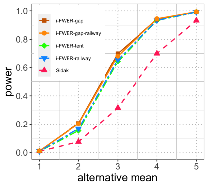
Figure 9: Power of the i-FWER test with the tent function (p=0.1subscript𝑝0.1p_{*}=0.1) and the gap function (pl=0.1,pu=0.5formulae-sequencesubscript𝑝𝑙0.1subscript𝑝𝑢0.5p_{l}=0.1,p_{u}=0.5). The gap function leads to slight improvement in power. Simulation follows the setting in Section Setting.

4.3 The “gap-railway” function

Combining the idea of the gap and railway functions, we develop the “gap-railway” function such that the middle p𝑝p-values are directly unmasked and the map g𝑔g for large p𝑝p-values is an increasing function (see Figure 7(d)). Given parameters plsubscript𝑝𝑙p_{l} and pusubscript𝑝𝑢p_{u}, the gap-railway function is defined as

h(Pi)=subscript𝑃𝑖absent\displaystyle h(P_{i})=~{} {1,0Pi<pl,1,pu<Pi1;cases10subscript𝑃𝑖subscript𝑝𝑙1subscript𝑝𝑢subscript𝑃𝑖1\displaystyle\begin{cases}1,&0\leq P_{i}<p_{l},\\ -1,&p_{u}<P_{i}\leq 1;\end{cases}{}
and g(Pi)=and 𝑔subscript𝑃𝑖absent\displaystyle\text{and }g(P_{i})=~{} {Pi,0Pi<pl,pl1pu(Pipu),pu<Pi1.casessubscript𝑃𝑖0subscript𝑃𝑖subscript𝑝𝑙subscript𝑝𝑙1subscript𝑝𝑢subscript𝑃𝑖subscript𝑝𝑢subscript𝑝𝑢subscript𝑃𝑖1\displaystyle\begin{cases}P_{i},&0\leq P_{i}<p_{l},\\ \frac{p_{l}}{1-p_{u}}(P_{i}-p_{u}),&p_{u}<P_{i}\leq 1.\end{cases} (10)

Comparing with the tent function with p=plsubscript𝑝subscript𝑝𝑙p_{*}=p_{l}, the i-FWER test using the gap function additionally uses the entire p𝑝p-values in [pl,pu]subscript𝑝𝑙subscript𝑝𝑢[p_{l},p_{u}] for interaction, which leads to an increased power (see Figure 9). The same pattern is maintained when we flip the mappings for large p𝑝p-values, shown in the comparison of the railway function and the gap-railway function444The tests with the tent function and the railway function have similar power; and same for the gap function and the gap-railway function. As the null p𝑝p-values follow an exact uniform distribution, so flipping the map g𝑔g for large p𝑝p-values does not change the power.. This improvement also motivates why the i-FWER test progressively unmasks h(Pi)subscript𝑃𝑖h(P_{i}), in other words, to reveal as much information to the analyst as allowed at the current step. Unmasking the p𝑝p-values even for the hypotheses outside of the rejection set can improve the power, because they help the joint modeling of all the p𝑝p-values, especially when there is some non-null structure.

To summarize, we have presented four types of masking functions: tent, railway, gap, gap-railway (see Figure 7). Compared to the tent (gap) function, the railway (gap-railway) functions are more robust to conservative nulls. Compared with the tent (railway) function, the gap (gap-railway) function reveals more information to guide the shrinkage of tsubscript𝑡\mathcal{R}_{t}. Note however that the railway or gap function is not always better than the tent function. We may favor the tent function over the railway function when there are less p𝑝p-values close to one, and we may favor the tent function over the gap function when there is considerable prior knowledge to guide the shrinkage of tsubscript𝑡\mathcal{R}_{t}.

The above discussion has explored specific non-null structures and masking functions. A large variety of masking functions and their advantages are yet to be discovered.

5 A prototypical application to genetic data

Below, we further demonstrate the power of the i-FWER test using a real ‘airway dataset’, which is analyzed by Independent Hypothesis Weighting (IHW) [Ignatiadis et al., 2016] and AdaPT [Lei and Fithian, 2018]; these are (respectively) adaptive and interactive algorithms with FDR control for independent hypotheses. We compare the number of rejections made by a variant of the IHW with FWER control and the i-FWER test using the tent function with the masking parameter psubscript𝑝p_{*} chosen as α/20,α/10,α/2𝛼20𝛼10𝛼2\alpha/20,\alpha/10,\alpha/2, when the targeted FWER level α𝛼\alpha varies in (0.1,0.2,0.3)0.10.20.3(0.1,0.2,0.3).

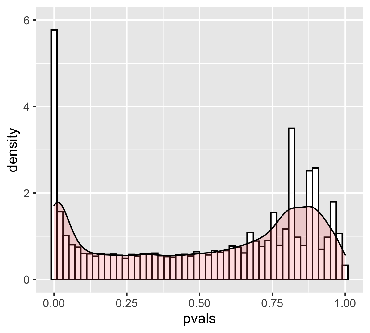
The airway data is an RNA-Seq dataset targeting the identification of differentially expressed genes in airway smooth muscle cell lines in response to dexamethasone, which contains 33469 genes (hypotheses) and a univariate covariate (the logarithm of normalized sample size) for each gene. The i-FWER test makes more rejections than the IHW for all considered FWER levels and all considered choices of psubscript𝑝p_{*} (see Table 1).

Table 1: Number of rejections by IHW and i-FWER test under different FWER levels.
level α𝛼\alpha IHW i-FWER
p=α/2subscript𝑝𝛼2p_{*}=\alpha/2 p=α/10subscript𝑝𝛼10p_{*}=\alpha/10 p=α/20subscript𝑝𝛼20p_{*}=\alpha/20
0.1 1552 1613 1681 1646
0.2 1645 1740 1849 1789
0.3 1708 1844 1925 1894

In hindsight, a small value for the masking parameter was more powerful in this dataset because over 1600 p𝑝p-values are extremely small (<105absentsuperscript105<10^{-5}), and these are highly likely to be the non-nulls. Thus, even when the masked p𝑝p-values for all hypotheses are in a small range, such as (0,0.01)00.01(0,0.01) when α=0.1𝛼0.1\alpha=0.1 and p=α/10subscript𝑝𝛼10p_{*}=\alpha/10, the p𝑝p-values from the non-nulls still stand out because they gather below 105superscript10510^{-5}. At the same time, the smaller the psubscript𝑝p_{*}, the more accurate (less conservative) is our estimate of FWER in (4); the algorithm can stop shrinking tsubscript𝑡\mathcal{R}_{t} earlier since more hypotheses with negative h(P)𝑃h(P) are allowed to be included in the final tsubscript𝑡\mathcal{R}_{t}. In practice, the choice of masking parameter can be guided by the prior belief of the strength of non-null signals: if the non-nulls have strong signal and hence extremely small p𝑝p-values (such as the mean value μ5𝜇5\mu\geq 5 when testing if a univariate Gaussian has zero mean), a small masking parameter is preferred; otherwise, we recommend α/2𝛼2\alpha/2 to leave more information for interactively shrinking the rejection set tsubscript𝑡\mathcal{R}_{t}.

6 Discussion

We proposed a multiple testing method with a valid FWER control while granting the analyst freedom of interacting with the revealed data. The masking function must be fixed in advance, but during the procedure of excluding possible nulls, the analyst can employ any model, heuristic, intuition, or domain knowledge, tailoring the algorithm to various applications. Although the validity requires an independence assumption, our method is a step forward to fulfilling the practical needs of allowing interactive human guidance to automated large-scale testing using ML in the sciences.

The critical idea that guarantees the FWER control is “masking and unmasking”. A series of interactive tests are developed following the idea of masking: Lei and Fithian [2018] and Lei et al. [2020] proposed the masking idea and an interactive test with FDR control; Duan et al. [2019] developed an interactive test for the global null; this work presents an interactive test with FWER control. At a high level, masking-based interactive testing achieves rigorous conclusions in an exploratory framework, giving this broad technique much appeal and potential.

Code and Data

Code can be found in https://github.com/duanby/i-FWER. It was tested on macOS using R (version 3.6.0) and the following packages: magrittr, splines, robustbase, ggplot2.

Data in Section 5 is collected by Himes et al. [2014] and available in R package airway. We follow Ignatiadis et al. [2016] and Lei and Fithian [2018] to analyze the data using DEseq2 package [Love et al., 2014].

Acknowledgements

We thank Jelle Goeman for his insightful comments on the connection between our proposed method and closed testing. We thank Will Fithian for related discussions. Eugene Katsevich, Ian Waudby-Smith, Jinjin Tian and Pratik Patil are acknowledged for their feedback on an early draft, and anonymous reviewers for helpful suggestions.

References

  • Barber and Candès [2015] Barber, R. F. and E. J. Candès (2015). Controlling the false discovery rate via knockoffs. The Annals of Statistics 43(5), 2055–2085.
  • Bretz et al. [2009] Bretz, F., W. Maurer, W. Brannath, and M. Posch (2009). A graphical approach to sequentially rejective multiple test procedures. Statistics in medicine 28(4), 586–604.
  • Duan et al. [2019] Duan, B., A. Ramdas, S. Balakrishnan, and L. Wasserman (2019). Interactive martingale tests for the global null. arXiv preprint arXiv:1909.07339.
  • Farcomeni [2008] Farcomeni, A. (2008). A review of modern multiple hypothesis testing, with particular attention to the false discovery proportion. Statistical methods in medical research 17(4), 347–388.
  • Goeman and Finos [2012] Goeman, J. J. and L. Finos (2012). The inheritance procedure: multiple testing of tree-structured hypotheses. Statistical applications in genetics and molecular biology 11(1), 1–18.
  • Goeman and Solari [2011] Goeman, J. J. and A. Solari (2011). Multiple testing for exploratory research. Statistical Science 26(4), 584–597.
  • Goeman and Solari [2014] Goeman, J. J. and A. Solari (2014). Multiple hypothesis testing in genomics. Statistics in medicine 33(11), 1946–1978.
  • Himes et al. [2014] Himes, B. E., X. Jiang, P. Wagner, R. Hu, Q. Wang, B. Klanderman, R. M. Whitaker, Q. Duan, J. Lasky-Su, and C. Nikolos (2014). RNA-Seq transcriptome profiling identifies crispld2 as a glucocorticoid responsive gene that modulates cytokine function in airway smooth muscle cells. PloS one 9(6), e99625.
  • Hochberg [1988] Hochberg, Y. (1988). A sharper bonferroni procedure for multiple tests of significance. Biometrika 75(4), 800–802.
  • Holm [1979] Holm, S. (1979). A simple sequentially rejective multiple test procedure. Scandinavian journal of statistics, 65–70.
  • Ignatiadis et al. [2016] Ignatiadis, N., B. Klaus, J. B. Zaugg, and W. Huber (2016). Data-driven hypothesis weighting increases detection power in genome-scale multiple testing. Nature methods 13(7), 577.
  • Janson and Su [2016] Janson, L. and W. Su (2016). Familywise error rate control via knockoffs. Electronic Journal of Statistics 10(1), 960–975.
  • Lei and Fithian [2018] Lei, L. and W. Fithian (2018). AdaPT: an interactive procedure for multiple testing with side information. Journal of the Royal Statistical Society: Series B (Statistical Methodology) 80(4), 649–679.
  • Lei et al. [2020] Lei, L., A. Ramdas, and W. Fithian (2020). STAR: A general interactive framework for FDR control under structural constraints. Biometrika (accepted).
  • Love et al. [2014] Love, M. I., W. Huber, and S. Anders (2014). Moderated estimation of fold change and dispersion for RNA-seq data with DESeq2. Genome biology 15(12), 550.
  • Marcus et al. [1976] Marcus, R., P. Eric, and K. R. Gabriel (1976). On closed testing procedures with special reference to ordered analysis of variance. Biometrika 63(3), 655–660.
  • Meinshausen [2008] Meinshausen, N. (2008). Hierarchical testing of variable importance. Biometrika 95(2), 265–278.
  • Šidák [1967] Šidák, Z. (1967). Rectangular confidence regions for the means of multivariate normal distributions. Journal of the American Statistical Association 62(318), 626–633.
  • Tamhane and Gou [2018] Tamhane, A. C. and J. Gou (2018). Advances in p𝑝p-value based multiple test procedures. Journal of biopharmaceutical statistics 28(1), 10–27.
  • Wiens and Dmitrienko [2005] Wiens, B. L. and A. Dmitrienko (2005). The fallback procedure for evaluating a single family of hypotheses. Journal of Biopharmaceutical Statistics 15(6), 929–942.
  • Zhao et al. [2019] Zhao, Q., D. S. Small, and W. Su (2019). Multiple testing when many p-values are uniformly conservative, with application to testing qualitative interaction in educational interventions. Journal of the American Statistical Association 114(527), 1291–1304.

Appendix A Distribution of the null p𝑝p-values

With tent masking, error control holds for null p𝑝p-values whose distribution satisfies a property called mirror-conservativeness:

f(a)f(11ppa), for all 0ap,formulae-sequence𝑓𝑎𝑓11subscript𝑝subscript𝑝𝑎 for all 0𝑎subscript𝑝f(a)\leq f\left(1-\frac{1-p_{*}}{p_{*}}a\right),\quad\text{ for all }0\leq a\leq p_{*}, (11)

where f𝑓f is the probability mass function of P𝑃P for discrete p𝑝p-values or the density function otherwise, and psubscript𝑝p_{*} is the parameter in Algorithm 1 (see proof in Appendix B). The mirror-conservativeness is first proposed by Lei and Fithian [2018] in the case of p=0.5subscript𝑝0.5p_{*}=0.5. A more commonly used notion of conservativeness is that p𝑝p-values are stochastically larger than uniform:

(Pa)a, for all 0a1,formulae-sequence𝑃𝑎𝑎 for all 0𝑎1\mathbb{P}(P\leq a)\leq a,\quad\text{ for all }0\leq a\leq 1,

which neither implies nor is implied by the mirror-conservativeness.

A sufficent condition of the mirror-conservativeness is that the p𝑝p-values have non-decreasing densities. For example, consider a one-dimensional exponential family and the hypotheses to test the value of its parameter θ𝜃\theta:

H0:θθ0, versus H1:θ>θ0,:subscript𝐻0𝜃subscript𝜃0 versus subscript𝐻1:𝜃subscript𝜃0H_{0}:\theta\leq\theta_{0},\quad\text{ versus }\quad H_{1}:\theta>\theta_{0},

where θ0subscript𝜃0\theta_{0} is a prespecified constant. The p𝑝p-value calculated from the uniformly most powerful test is shown to have a nondecreasing density [Zhao et al., 2019]; thus, it satisfies the mirror-conservativeness. The conservative nulls described in Section 4.1 also fall into the above category where the exponential family is Gaussian, and the parameter is the mean value. Indeed, when the p𝑝p-values have non-decreasing densities, the i-FWER test also has a valid error control using alternative masking functions as proposed in Section 4 (see proof in Appendix F).

Appendix B Proof of Theorem 1

The main idea of the proof is that the missing bits h(Pi)subscript𝑃𝑖h(P_{i}) of nulls are coin flips with probability psubscript𝑝p_{*} to be heads, so the number of false rejections (i.e. the number of nulls with h(Pi)=1subscript𝑃𝑖1h(P_{i})=1 before the number of hypotheses with h(Pi)=1subscript𝑃𝑖1h(P_{i})=-1 reaches a fixed number) is stochastically dominated by a negative binomial distribution. There are two main challenges. First, the interaction uses unmasked p𝑝p-value information to reorder h(Pi)subscript𝑃𝑖h(P_{i}), so it is not trivial to show that the reordered h(Pi)subscript𝑃𝑖h(P_{i}) preserve the same distribution as that before ordering. Second, our procedure runs backward to find the first time that the number of hypotheses with negative h(Pi)subscript𝑃𝑖h(P_{i}) is below a fixed number, which differs from the standard description of a negative binomial distribution.

B.1 Missing bits after interactive ordering

We first study the effect of interaction. Imagine that Algorithm 1 does not have a stopping rule and generates a full sequence of tsubscript𝑡\mathcal{R}_{t} for t=0,1,n𝑡01𝑛t=0,1,\ldots n, where 0=[n]subscript0delimited-[]𝑛\mathcal{R}_{0}=[n] and n=subscript𝑛\mathcal{R}_{n}=\emptyset. It leads to an ordered sequence of h(Pi)subscript𝑃𝑖h(P_{i}):

h(Pπ1),h(Pπ2),,h(Pπn),subscript𝑃subscript𝜋1subscript𝑃subscript𝜋2subscript𝑃subscript𝜋𝑛h(P_{\pi_{1}}),h(P_{\pi_{2}}),\ldots,h(P_{\pi_{n}}),

where πnsubscript𝜋𝑛\pi_{n} is the index of the first excluded hypothesis and πjsubscript𝜋𝑗\pi_{j} denotes the index of the hypothesis excluded at step nj+1𝑛𝑗1n-j+1, that is πj=nj\nj+1subscript𝜋𝑗\subscript𝑛𝑗subscript𝑛𝑗1\pi_{j}=\mathcal{R}_{n-j}\backslash\mathcal{R}_{n-j+1}.

Lemma 1.

Suppose the null p𝑝p-values are uniformly distributed and all the hypotheses are nulls, then for any j=1,,n𝑗1𝑛j=1,\ldots,n,

𝔼[𝟙(h(Pπj)=1)]=p,𝔼delimited-[]1subscript𝑃subscript𝜋𝑗1subscript𝑝\mathbb{E}\left[\mathbbm{1}\left(h(P_{\pi_{j}})=1\right)\right]=p_{*},

and {𝟙(h(Pπj)=1)}j=1nsuperscriptsubscript1subscript𝑃subscript𝜋𝑗1𝑗1𝑛\{\mathbbm{1}\left(h(P_{\pi_{j}})=1\right)\}_{j=1}^{n} are mutually independent.

Proof.

Recall that the available information for the analyst to choose πjsubscript𝜋𝑗\pi_{j} is nj=σ({xi,g(Pi)}i=1n,{Pi}inj)subscript𝑛𝑗𝜎superscriptsubscriptsubscript𝑥𝑖𝑔subscript𝑃𝑖𝑖1𝑛subscriptsubscript𝑃𝑖𝑖subscript𝑛𝑗{\mathcal{F}_{n-j}=\sigma\Big{(}\{x_{i},g(P_{i})\}_{i=1}^{n},\{P_{i}\}_{i\notin\mathcal{R}_{n-j}}\Big{)}}. First, consider the conditional expectation:

𝔼[𝟙(h(Pπj)=1)|nj]\displaystyle\mathbb{E}\left[\mathbbm{1}\left(h(P_{\pi_{j}})=1\right)\middle|\mathcal{F}_{n-j}\right]{}
=\displaystyle=~{} i[n]𝔼[𝟙(h(Pπj)=1)|πj=i,nj](πj=i|nj)\displaystyle\sum_{i\in[n]}\mathbb{E}\left[\mathbbm{1}\left(h(P_{\pi_{j}})=1\right)\middle|\pi_{j}=i,\mathcal{F}_{n-j}\right]\mathbb{P}\left(\pi_{j}=i\middle|\mathcal{F}_{n-j}\right){}
=(a)𝑎\displaystyle\overset{(a)}{=}~{} inj𝔼[𝟙(h(Pi)=1)|πj=i,nj](πj=i|nj)\displaystyle\sum_{i\in\mathcal{R}_{n-j}}\mathbb{E}\left[\mathbbm{1}\left(h(P_{i})=1\right)\middle|\pi_{j}=i,\mathcal{F}_{n-j}\right]\mathbb{P}\left(\pi_{j}=i\middle|\mathcal{F}_{n-j}\right){}
=(b)𝑏\displaystyle\overset{(b)}{=}~{} inj𝔼[𝟙(h(Pi)=1)|nj](πj=i|nj)\displaystyle\sum_{i\in\mathcal{R}_{n-j}}\mathbb{E}\left[\mathbbm{1}\left(h(P_{i})=1\right)\middle|\mathcal{F}_{n-j}\right]\mathbb{P}\left(\pi_{j}=i\middle|\mathcal{F}_{n-j}\right){}
=(c)𝑐\displaystyle\overset{(c)}{=}~{} inj𝔼[𝟙(h(Pi)=1)](πj=i|nj)\displaystyle\sum_{i\in\mathcal{R}_{n-j}}\mathbb{E}\left[\mathbbm{1}\left(h(P_{i})=1\right)\right]\mathbb{P}\left(\pi_{j}=i\middle|\mathcal{F}_{n-j}\right){}
=\displaystyle=~{} pinj(πj=i|nj)=p,\displaystyle p_{*}\sum_{i\in\mathcal{R}_{n-j}}\mathbb{P}\left(\pi_{j}=i\middle|\mathcal{F}_{n-j}\right)=p_{*}, (12)

where equation (a)𝑎(a) narrows down the choice of i𝑖i because (πj=inj)=0subscript𝜋𝑗conditional𝑖subscript𝑛𝑗0\mathbb{P}(\pi_{j}=i\mid\mathcal{F}_{n-j})=0 for any inj𝑖subscript𝑛𝑗i\notin\mathcal{R}_{n-j}; equation (b)𝑏(b) drops the condition of πj=isubscript𝜋𝑗𝑖\pi_{j}=i because πjsubscript𝜋𝑗\pi_{j} is measurable with respect to njsubscript𝑛𝑗\mathcal{F}_{n-j}; and equation (c)𝑐(c) drops the condition njsubscript𝑛𝑗\mathcal{F}_{n-j} because by the independence assumptions in Theorem 1, h(Pi)subscript𝑃𝑖h(P_{i}) is independent of njsubscript𝑛𝑗\mathcal{F}_{n-j} for any inj𝑖subscript𝑛𝑗i\in\mathcal{R}_{n-j}.

Therefore, by the law of iterated expectations, we prove the claim on expected value:

𝔼[𝟙(h(Pπj)=1)]=𝔼[𝔼[𝟙(h(Pπj)=1)|nj]]=p.\mathbb{E}\left[\mathbbm{1}\left(h(P_{\pi_{j}})=1\right)\right]=\mathbb{E}\left[\mathbb{E}\left[\mathbbm{1}\left(h(P_{\pi_{j}})=1\right)\middle|\mathcal{F}_{n-j}\right]\right]=p_{*}.

For mutual independence, we can show that for any 1k<jn1𝑘𝑗𝑛1\leq k<j\leq n, 𝟙(h(Pπk)=1)1subscript𝑃subscript𝜋𝑘1\mathbbm{1}\left(h(P_{\pi_{k}})=1\right) is independent of 𝟙(h(Pπj)=1)1subscript𝑃subscript𝜋𝑗1\mathbbm{1}\left(h(P_{\pi_{j}})=1\right). Consider the conditional expectation:

𝔼[𝟙(h(Pπk)=1)|𝟙(h(Pπj)=1)]\displaystyle\mathbb{E}\left[\mathbbm{1}\left(h(P_{\pi_{k}})=1\right)\middle|\mathbbm{1}\left(h(P_{\pi_{j}})=1\right)\right]{}
=\displaystyle=~{} 𝔼[𝔼[𝟙(h(Pπk)=1)|nk,𝟙(h(Pπj)=1)]|𝟙(h(Pπj)=1)]\displaystyle\mathbb{E}\left[\mathbb{E}\left[\mathbbm{1}\left(h(P_{\pi_{k}})=1\right)\middle|\mathcal{F}_{n-k},\mathbbm{1}\left(h(P_{\pi_{j}})=1\right)\right]\middle|\mathbbm{1}\left(h(P_{\pi_{j}})=1\right)\right]{}
(note that 𝟙(h(Pπj)=1) is measurable with respect to nk)(note that 1subscript𝑃subscript𝜋𝑗1 is measurable with respect to subscript𝑛𝑘)\displaystyle\text{(note that }\mathbbm{1}\left(h(P_{\pi_{j}})=1\right)\text{ is measurable with respect to }\mathcal{F}_{n-k}\text{)}{}
=\displaystyle=~{} 𝔼[𝔼[𝟙(h(Pπk)=1)|nk]|𝟙(h(Pπj)=1)]\displaystyle\mathbb{E}\left[\mathbb{E}\left[\mathbbm{1}\left(h(P_{\pi_{k}})=1\right)\middle|\mathcal{F}_{n-k}\right]\middle|\mathbbm{1}\left(h(P_{\pi_{j}})=1\right)\right]{}
(use equation (B.1) for the conditional expectation)
=\displaystyle=~{} 𝔼[p𝟙(h(Pπj)=1)]=p.𝔼delimited-[]conditionalsubscript𝑝1subscript𝑃subscript𝜋𝑗1subscript𝑝\displaystyle\mathbb{E}\left[p_{*}\mid\mathbbm{1}\left(h(P_{\pi_{j}})=1\right)\right]=p_{*}.

It follows that 𝟙(h(Pπk)=1)𝟙(h(Pπj)=1)conditional1subscript𝑃subscript𝜋𝑘11subscript𝑃subscript𝜋𝑗1\mathbbm{1}\left(h(P_{\pi_{k}})=1\right)\mid\mathbbm{1}\left(h(P_{\pi_{j}})=1\right) is a Bernoulli with parameter psubscript𝑝p_{*}, same as the marginal distribution of 𝟙(h(Pπk)=1)1subscript𝑃subscript𝜋𝑘1\mathbbm{1}\left(h(P_{\pi_{k}})=1\right); thus, 𝟙(h(Pπk)=1)1subscript𝑃subscript𝜋𝑘1\mathbbm{1}\left(h(P_{\pi_{k}})=1\right) is independent of 𝟙(h(Pπj)=1)1subscript𝑃subscript𝜋𝑗1\mathbbm{1}\left(h(P_{\pi_{j}})=1\right) for any 1k<jn1𝑘𝑗𝑛1\leq k<j\leq n as stated in the Lemma. ∎

Corollary 1.

Suppose the null p𝑝p-values are uniformly distributed and there may exist non-nulls. For any j=1,,n𝑗1𝑛j=1,\ldots,n,

𝔼[𝟙(h(Pπj)=1)|{𝟙(h(Pπk)=1)}k=j+1n,{𝟙(πk0)}k=j+1n,πj0]=p,\mathbb{E}\left[\mathbbm{1}\left(h(P_{\pi_{j}})=1\right)\middle|\left\{\mathbbm{1}\left(h(P_{\pi_{k}})=1\right)\right\}_{k=j+1}^{n},\left\{\mathbbm{1}\left(\pi_{k}\in\mathcal{H}_{0}\right)\right\}_{k=j+1}^{n},\pi_{j}\in\mathcal{H}_{0}\right]=p_{*},

where {πk}k=j+1nsuperscriptsubscriptsubscript𝜋𝑘𝑘𝑗1𝑛\{\pi_{k}\}_{k=j+1}^{n} represents the hypotheses excluded before πjsubscript𝜋𝑗\pi_{j}.

Proof.

Denote the condition σ({𝟙(h(Pπk)=1)}k=j+1n,{𝟙(πk0)}k=j+1n)𝜎superscriptsubscript1subscript𝑃subscript𝜋𝑘1𝑘𝑗1𝑛superscriptsubscript1subscript𝜋𝑘subscript0𝑘𝑗1𝑛\sigma\left(\left\{\mathbbm{1}\left(h(P_{\pi_{k}})=1\right)\right\}_{k=j+1}^{n},\left\{\mathbbm{1}\left(\pi_{k}\in\mathcal{H}_{0}\right)\right\}_{k=j+1}^{n}\right) as njhsuperscriptsubscript𝑛𝑗\mathcal{F}_{n-j}^{h}. The proof is similar to Lemma 1. First, consider the expectation conditional on njsubscript𝑛𝑗\mathcal{F}_{n-j}:

𝔼[𝟙(h(Pπj)=1)|njh,πj0,nj]\displaystyle\mathbb{E}\left[\mathbbm{1}\left(h(P_{\pi_{j}})=1\right)\middle|\mathcal{F}_{n-j}^{h},\pi_{j}\in\mathcal{H}_{0},\mathcal{F}_{n-j}\right]{}
=\displaystyle=~{} 𝔼[𝟙(h(Pπj)=1)|πj0,nj](since njh is a subset of nj)\displaystyle\mathbb{E}\left[\mathbbm{1}\left(h(P_{\pi_{j}})=1\right)\middle|\pi_{j}\in\mathcal{H}_{0},\mathcal{F}_{n-j}\right]\quad(\text{since }\mathcal{F}_{n-j}^{h}\text{ is a subset of }\mathcal{F}_{n-j}){}
=\displaystyle=~{} i[n]𝔼[𝟙(h(Pi)=1)πj=i,πj0,nj](πj=iπj0,nj)\displaystyle\sum_{i\in[n]}\mathbb{E}\left[\mathbbm{1}\left(h(P_{i})=1\right)\mid\pi_{j}=i,\pi_{j}\in\mathcal{H}_{0},\mathcal{F}_{n-j}\right]\mathbb{P}(\pi_{j}=i\mid\pi_{j}\in\mathcal{H}_{0},\mathcal{F}_{n-j}){}
=\displaystyle=~{} inj0𝔼[𝟙(h(Pi)=1)πj=i,πj0,nj](πj=iπj0,nj)\displaystyle\sum_{i\in\mathcal{R}_{n-j}\cap\mathcal{H}_{0}}\mathbb{E}\left[\mathbbm{1}\left(h(P_{i})=1\right)\mid\pi_{j}=i,\pi_{j}\in\mathcal{H}_{0},\mathcal{F}_{n-j}\right]\mathbb{P}(\pi_{j}=i\mid\pi_{j}\in\mathcal{H}_{0},\mathcal{F}_{n-j}){}
=\displaystyle=~{} inj0𝔼[𝟙(h(Pi)=1)|nj](πj=iπj0,nj)\displaystyle\sum_{i\in\mathcal{R}_{n-j}\cap\mathcal{H}_{0}}\mathbb{E}\left[\mathbbm{1}\left(h(P_{i})=1\right)\middle|\mathcal{F}_{n-j}\right]\mathbb{P}(\pi_{j}=i\mid\pi_{j}\in\mathcal{H}_{0},\mathcal{F}_{n-j}){}
=\displaystyle=~{} pinj0(πj=iπj0,nj)=p,\displaystyle p_{*}\sum_{i\in\mathcal{R}_{n-j}\cap\mathcal{H}_{0}}\mathbb{P}(\pi_{j}=i\mid\pi_{j}\in\mathcal{H}_{0},\mathcal{F}_{n-j})=p_{*}, (13)

where we use the same technics of proving equation (B.1).

Thus, by the law of iterated expectations, we have

𝔼[𝟙(h(Pπj)=1)|njh,πj0]\displaystyle\mathbb{E}\left[\mathbbm{1}\left(h(P_{\pi_{j}})=1\right)\middle|\mathcal{F}_{n-j}^{h},\pi_{j}\in\mathcal{H}_{0}\right]{}
=\displaystyle=~{} 𝔼[𝔼[𝟙(h(Pπj)=1)|njh,πj0,nj]|njh,πj0]=p,\displaystyle\mathbb{E}\left[\mathbb{E}\left[\mathbbm{1}\left(h(P_{\pi_{j}})=1\right)\middle|\mathcal{F}_{n-j}^{h},\pi_{j}\in\mathcal{H}_{0},\mathcal{F}_{n-j}\right]\middle|\mathcal{F}_{n-j}^{h},\pi_{j}\in\mathcal{H}_{0}\right]=p_{*},

which completes the proof. ∎

Corollary 2.

Suppose the null p𝑝p-values can be mirror-conservative as defined in (11) and there may exist non-nulls, then for any j=1,,n𝑗1𝑛j=1,\ldots,n,

𝔼[𝟙(h(Pπj)=1)|{𝟙(h(Pπk)=1)}k=j+1n,{𝟙(πk0)}k=j+1n,πj0,{g(Pπk)}k=1n]p,\mathbb{E}\left[\mathbbm{1}\left(h(P_{\pi_{j}})=1\right)\middle|\left\{\mathbbm{1}\left(h(P_{\pi_{k}})=1\right)\right\}_{k=j+1}^{n},\left\{\mathbbm{1}\left(\pi_{k}\in\mathcal{H}_{0}\right)\right\}_{k=j+1}^{n},\pi_{j}\in\mathcal{H}_{0},\{g(P_{\pi_{k}})\}_{k=1}^{n}\right]\leq p_{*},

where {g(Pπk)}k=1nsuperscriptsubscript𝑔subscript𝑃subscript𝜋𝑘𝑘1𝑛\{g(P_{\pi_{k}})\}_{k=1}^{n} denotes g(P)𝑔𝑃g(P) for all the hypotheses (excluded or not).

Proof.

First, we claim that a mirror-conservative p𝑝p-value P𝑃P satisfies that

𝔼[𝟙(h(P)=1)g(P)]p,𝔼delimited-[]conditional1𝑃1𝑔𝑃subscript𝑝\displaystyle\mathbb{E}\left[\mathbbm{1}\left(h(P)=1\right)\mid g(P)\right]\leq p_{*}, (14)

since for every a(0,p)𝑎0subscript𝑝a\in(0,p_{*}),

𝔼[𝟙(h(P)=1)g(P)=a]𝔼delimited-[]conditional1𝑃1𝑔𝑃𝑎\displaystyle\mathbb{E}\left[\mathbbm{1}\left(h(P)=1\right)\mid g(P)=a\right]{}
=\displaystyle=~{} pf(a)pf(a)+(1p)f(11ppa)subscript𝑝𝑓𝑎subscript𝑝𝑓𝑎1subscript𝑝𝑓11subscript𝑝subscript𝑝𝑎\displaystyle\frac{p_{*}f(a)}{p_{*}f(a)+(1-p_{*})f\left(1-\frac{1-p_{*}}{p_{*}}a\right)}{}
=\displaystyle=~{} pp+(1p)f(11ppa)/f(a)p,subscript𝑝subscript𝑝1subscript𝑝𝑓11subscript𝑝subscript𝑝𝑎𝑓𝑎subscript𝑝\displaystyle\frac{p_{*}}{p_{*}+(1-p_{*})f\left(1-\frac{1-p_{*}}{p_{*}}a\right)/f(a)}\leq p_{*},

where recall that f𝑓f is the probability mass function of P𝑃P for discrete p𝑝p-values or the density function otherwise. The last inequality comes from the definition of mirror-conservativeness in (11). The rest of the proof is similar to Corollary 1, where we first condition on njsubscript𝑛𝑗\mathcal{F}_{n-j}:

𝔼[𝟙(h(Pπj)=1)|nj,njh,πj0,{g(Pπk)}k=1n]\displaystyle\mathbb{E}\left[\mathbbm{1}\left(h(P_{\pi_{j}})=1\right)\middle|\mathcal{F}_{n-j},\mathcal{F}_{n-j}^{h},\pi_{j}\in\mathcal{H}_{0},\{g(P_{\pi_{k}})\}_{k=1}^{n}\right]{}
=\displaystyle=~{} ini0𝔼[𝟙(h(Pi)=1)nj](πj=i|nj,njh,πj0,{g(Pπk)}k=1n)\displaystyle\sum_{i\in\mathcal{R}_{n-i}\cap\mathcal{H}_{0}}\mathbb{E}\left[\mathbbm{1}\left(h(P_{i})=1\right)\mid\mathcal{F}_{n-j}\right]\mathbb{P}\left(\pi_{j}=i\middle|\mathcal{F}_{n-j},\mathcal{F}_{n-j}^{h},\pi_{j}\in\mathcal{H}_{0},\{g(P_{\pi_{k}})\}_{k=1}^{n}\right){}
=(a)𝑎\displaystyle\overset{(a)}{=}~{} ini0𝔼[𝟙(h(Pi)=1)g(Pi)](πj=i|nj,njh,πj0,{g(Pπk)}k=1n)\displaystyle\sum_{i\in\mathcal{R}_{n-i}\cap\mathcal{H}_{0}}\mathbb{E}\left[\mathbbm{1}\left(h(P_{i})=1\right)\mid g(P_{i})\right]\mathbb{P}\left(\pi_{j}=i\middle|\mathcal{F}_{n-j},\mathcal{F}_{n-j}^{h},\pi_{j}\in\mathcal{H}_{0},\{g(P_{\pi_{k}})\}_{k=1}^{n}\right){}
\displaystyle\leq~{} pini0(πj=i|nj,njh,πj0,{g(Pπk)}k=1n)=p,\displaystyle p_{*}\sum_{i\in\mathcal{R}_{n-i}\cap\mathcal{H}_{0}}\mathbb{P}\left(\pi_{j}=i\middle|\mathcal{F}_{n-j},\mathcal{F}_{n-j}^{h},\pi_{j}\in\mathcal{H}_{0},\{g(P_{\pi_{k}})\}_{k=1}^{n}\right)=p_{*},

where equation (a)𝑎(a) simplify the condition of njsubscript𝑛𝑗\mathcal{F}_{n-j} to g(Pi)𝑔subscript𝑃𝑖g(P_{i}) because for any ini0𝑖subscript𝑛𝑖subscript0i\in\mathcal{R}_{n-i}\cap\mathcal{H}_{0}, h(Pi)subscript𝑃𝑖h(P_{i}) is independent of other information in njsubscript𝑛𝑗\mathcal{F}_{n-j}.

Then, by the law of iterated expectations, we obtain

𝔼[𝟙(h(Pπj)=1)|njh,πj0,{g(Pπk)}k=1n]\displaystyle\mathbb{E}\left[\mathbbm{1}\left(h(P_{\pi_{j}})=1\right)\middle|\mathcal{F}_{n-j}^{h},\pi_{j}\in\mathcal{H}_{0},\{g(P_{\pi_{k}})\}_{k=1}^{n}\right]{}
=\displaystyle=~{} 𝔼[𝔼[𝟙(h(Pπj)=1)|nj,njh,πj0,{g(Pπk)}k=1n]|njh,πj0,{g(Pπk)}k=1n]p,\displaystyle\mathbb{E}\left[\mathbb{E}\left[\mathbbm{1}\left(h(P_{\pi_{j}})=1\right)\middle|\mathcal{F}_{n-j},\mathcal{F}_{n-j}^{h},\pi_{j}\in\mathcal{H}_{0},\{g(P_{\pi_{k}})\}_{k=1}^{n}\right]\middle|\mathcal{F}_{n-j}^{h},\pi_{j}\in\mathcal{H}_{0},\{g(P_{\pi_{k}})\}_{k=1}^{n}\right]\leq p_{*},

thus the proof is completed. ∎

B.2 Negative binomial distribution

In this section, we discuss several procedures for Bernoulli trials (coin flips) and their connections with the negative binomial distribution.

Lemma 2.

Suppose A1,,Ansubscript𝐴1subscript𝐴𝑛A_{1},\ldots,A_{n} are i.i.d. Bernoulli with parameter psubscript𝑝p_{*}. For t=1,,n𝑡1𝑛t=1,\ldots,n, consider the sum Mt=j=1tAjsubscript𝑀𝑡superscriptsubscript𝑗1𝑡subscript𝐴𝑗{M_{t}=\sum_{j=1}^{t}A_{j}} and the filtration 𝒢to=σ({Aj}j=1t)superscriptsubscript𝒢𝑡𝑜𝜎superscriptsubscriptsubscript𝐴𝑗𝑗1𝑡\mathcal{G}_{t}^{o}=\sigma\left(\{A_{j}\}_{j=1}^{t}\right). Define a stopping time parameterized by a constant v(1)annotated𝑣absent1v(\geq 1):

τo=min{0<tn:tMtv or t=n},superscript𝜏𝑜:0𝑡𝑛𝑡subscript𝑀𝑡𝑣 or 𝑡𝑛\displaystyle\tau^{o}=\min\{0<t\leq n:t-M_{t}\geq v\text{ or }t=n\}, (15)

then Mτosubscript𝑀superscript𝜏𝑜M_{\tau^{o}} is stochastically dominated by a negative binomial distribution:

MτoNB(v,p).precedes-or-equalssubscript𝑀superscript𝜏𝑜NB𝑣subscript𝑝M_{\tau^{o}}\preceq\mathrm{NB}(v,p_{*}).
Proof.

Recall that the negative binomial NB(v,p)NB𝑣subscript𝑝\mathrm{NB}(v,p_{*}) is the distribution of the number of success in a sequence of independent and identically distributed Bernoulli trials with probability psubscript𝑝p_{*} before a predefined number v𝑣v of failures have occurred. Imagine the sequence of Ajsubscript𝐴𝑗A_{j} is extended to infinitely many Bernoulli trials: A1,,An,An+1,subscript𝐴1subscript𝐴𝑛subscriptsuperscript𝐴𝑛1A_{1},\ldots,A_{n},A^{\prime}_{n+1},\ldots, where {Aj}j=n+1superscriptsubscriptsubscriptsuperscript𝐴𝑗𝑗𝑛1\{A^{\prime}_{j}\}_{j=n+1}^{\infty} are also i.i.d. Bernoulli with parameter psubscript𝑝p_{*} and they are independent of {Aj}j=1nsuperscriptsubscriptsubscript𝐴𝑗𝑗1𝑛\{A_{j}\}_{j=1}^{n}. Let U𝑈U be the number of success before v𝑣v-th failure, then by definition, U𝑈U follows a negative binomial distribution NB(v,p)NB𝑣subscript𝑝\mathrm{NB}(v,p_{*}). We can rewrite U𝑈U as a sum at a stopping time: UMτ𝑈subscript𝑀superscript𝜏U\equiv M_{\tau^{\prime}}, where τ=min{t>0:tMtv}superscript𝜏:𝑡0𝑡subscript𝑀𝑡𝑣{\tau^{\prime}=\min\{t>0}:t-M_{t}\geq v\}. By definition, τoτsuperscript𝜏𝑜superscript𝜏\tau^{o}\leq\tau^{\prime} (a.s.), which indicates MτoMτsubscript𝑀superscript𝜏𝑜subscript𝑀superscript𝜏M_{\tau^{o}}\leq M_{\tau^{\prime}} because Mtsubscript𝑀𝑡M_{t} is nondecreasing with respect to t𝑡t. Thus, we have proved that MτoNB(v,p)precedes-or-equalssubscript𝑀superscript𝜏𝑜NB𝑣subscript𝑝M_{\tau^{o}}\preceq\mathrm{NB}(v,p_{*}). ∎

Corollary 3.

Following the setting in Lemma 2, we consider the shrinking sum Mt~=j=1ntAj~subscript𝑀𝑡superscriptsubscript𝑗1𝑛𝑡subscript𝐴𝑗\widetilde{M_{t}}=\sum_{j=1}^{n-t}A_{j} for t=0,1,,n1𝑡01𝑛1t=0,1,\ldots,n-1. Let the filtration be 𝒢t~=σ(Mt~,{Aj}j=nt+1n)~subscript𝒢𝑡𝜎~subscript𝑀𝑡superscriptsubscriptsubscript𝐴𝑗𝑗𝑛𝑡1𝑛\widetilde{\mathcal{G}_{t}}=\sigma\left(\widetilde{M_{t}},\{A_{j}\}_{j=n-t+1}^{n}\right). Given a constant v(1)annotated𝑣absent1v(\geq 1), we define a stopping time:

τ~=min{0t<n:(nt)Mt~<v or t=n1},~𝜏:0𝑡𝑛𝑛𝑡~subscript𝑀𝑡𝑣 or 𝑡𝑛1\displaystyle\widetilde{\tau}=\min\{0\leq t<n:(n-t)-\widetilde{M_{t}}<v\text{ or }t=n-1\}, (16)

then it still holds that Mτ~~NB(v,p)precedes-or-equals~subscript𝑀~𝜏NB𝑣subscript𝑝\widetilde{M_{\widetilde{\tau}}}\preceq\mathrm{NB}(v,p_{*}).

Proof.

We first replace the notion of time t𝑡t by ns𝑛𝑠n-s, and let time runs backward: s=n,n1,,1𝑠𝑛𝑛11s=n,n-1,\ldots,1. The above setting can be rewritten as Mt~(=j=1ntAj)MntMsannotated~subscript𝑀𝑡absentsuperscriptsubscript𝑗1𝑛𝑡subscript𝐴𝑗subscript𝑀𝑛𝑡subscript𝑀𝑠\widetilde{M_{t}}(=\sum_{j=1}^{n-t}A_{j})\equiv M_{n-t}\equiv M_{s} and 𝒢t~=σ(Ms,{Aj}j=s+1n)=:𝒢sb\widetilde{\mathcal{G}_{t}}=\sigma\left(M_{s},\{A_{j}\}_{j=s+1}^{n}\right)=:\mathcal{G}_{s}^{b}. Define a stopping time:

τb=max{0<sn:sMs<v or s=1},superscript𝜏𝑏:0𝑠𝑛𝑠subscript𝑀𝑠𝑣 or 𝑠1\displaystyle\tau^{b}=\max\{0<s\leq n:s-M_{s}<v\text{ or }s=1\}, (17)

which runs backward with respect to the filtration 𝒢sbsuperscriptsubscript𝒢𝑠𝑏\mathcal{G}_{s}^{b}. By definition, we have nτ~τb𝑛~𝜏superscript𝜏𝑏n-\widetilde{\tau}\equiv\tau^{b}, and hence Mτ~~Mτb~subscript𝑀~𝜏subscript𝑀superscript𝜏𝑏\widetilde{M_{\widetilde{\tau}}}\equiv M_{\tau^{b}}.

Now, we show that MτbMτosubscript𝑀superscript𝜏𝑏subscript𝑀superscript𝜏𝑜M_{\tau^{b}}\equiv M_{\tau^{o}} for τosuperscript𝜏𝑜\tau^{o} defined in Lemma 2. First, consider two edge cases: (1) if tMt<v𝑡subscript𝑀𝑡𝑣t-M_{t}<v holds for every 0<tn0𝑡𝑛0<t\leq n, then τb=n=τosuperscript𝜏𝑏𝑛superscript𝜏𝑜\tau^{b}=n=\tau^{o}, and thus Mτb=Mτosubscript𝑀superscript𝜏𝑏subscript𝑀superscript𝜏𝑜M_{\tau^{b}}=M_{\tau^{o}}; (2) if tMtv𝑡subscript𝑀𝑡𝑣t-M_{t}\geq v holds for every 0<tn0𝑡𝑛0<t\leq n, then τb=1=τosuperscript𝜏𝑏1superscript𝜏𝑜\tau^{b}=1=\tau^{o}, and again Mτb=Mτosubscript𝑀superscript𝜏𝑏subscript𝑀superscript𝜏𝑜M_{\tau^{b}}=M_{\tau^{o}}. Next, consider the case where tMt<v𝑡subscript𝑀𝑡𝑣t-M_{t}<v for some t𝑡t, and tMtv𝑡subscript𝑀𝑡𝑣t-M_{t}\geq v for some other t𝑡t. Note that by definition, τb+1superscript𝜏𝑏1\tau^{b}+1 is a stopping time with respect to 𝒢tosuperscriptsubscript𝒢𝑡𝑜\mathcal{G}_{t}^{o}, and τb+1=τosuperscript𝜏𝑏1superscript𝜏𝑜\tau^{b}+1=\tau^{o}. Also, note that by the definition of τosuperscript𝜏𝑜\tau^{o}, we have Aτo=0subscript𝐴superscript𝜏𝑜0A_{\tau^{o}}=0, so Mτo1=Mτosubscript𝑀superscript𝜏𝑜1subscript𝑀superscript𝜏𝑜M_{\tau^{o}-1}=M_{\tau^{o}}. Thus, Mτb=Mτo1=Mτosubscript𝑀superscript𝜏𝑏subscript𝑀superscript𝜏𝑜1subscript𝑀superscript𝜏𝑜M_{\tau^{b}}=M_{\tau^{o}-1}=M_{\tau^{o}}. Therefore, by Lemma 2, Mτ~~MτbMτoNB(v,p)~subscript𝑀~𝜏subscript𝑀superscript𝜏𝑏subscript𝑀superscript𝜏𝑜precedes-or-equals𝑁𝐵𝑣subscript𝑝\widetilde{M_{\widetilde{\tau}}}\equiv M_{\tau^{b}}\equiv M_{\tau^{o}}\preceq NB(v,p_{*}), as stated in the above Corollary. ∎

Corollary 4.

Consider a weighted version of the setting in Corollary 3. Let the weights {Wj}j=1nsuperscriptsubscriptsubscript𝑊𝑗𝑗1𝑛\{W_{j}\}_{j=1}^{n} be a sequence of Bernoulli, such that (a) j=1nWj=msuperscriptsubscript𝑗1𝑛subscript𝑊𝑗𝑚\sum_{j=1}^{n}W_{j}=m for a fixed constant mn𝑚𝑛m\leq n; and (b) Ajσ({Ak,Wk}k=j+1n,Wj=1)conditionalsubscript𝐴𝑗𝜎superscriptsubscriptsubscript𝐴𝑘subscript𝑊𝑘𝑘𝑗1𝑛subscript𝑊𝑗1A_{j}\mid\sigma\left(\{A_{k},W_{k}\}_{k=j+1}^{n},W_{j}=1\right) is a Bernoulli with parameter psubscript𝑝p_{*}. Consider the sum Mtw=j=1ntWjAjsuperscriptsubscript𝑀𝑡𝑤superscriptsubscript𝑗1𝑛𝑡subscript𝑊𝑗subscript𝐴𝑗M_{t}^{w}=\sum_{j=1}^{n-t}W_{j}A_{j}. Given a constant v(1)annotated𝑣absent1v(\geq 1), we define a stopping time:

τw=superscript𝜏𝑤absent\displaystyle\tau^{w}=~{} min{0t<n:j=1ntWj(1Aj)<v or t=n1}:0𝑡𝑛superscriptsubscript𝑗1𝑛𝑡subscript𝑊𝑗1subscript𝐴𝑗𝑣 or 𝑡𝑛1\displaystyle\min\{0\leq t<n:\sum_{j=1}^{n-t}W_{j}(1-A_{j})<v\text{ or }t=n-1\}{} (18)
\displaystyle\equiv~{} min{0t<n:j=1ntWjMtw<v or t=n1},:0𝑡𝑛superscriptsubscript𝑗1𝑛𝑡subscript𝑊𝑗superscriptsubscript𝑀𝑡𝑤𝑣 or 𝑡𝑛1\displaystyle\min\{0\leq t<n:\sum_{j=1}^{n-t}W_{j}-M_{t}^{w}<v\text{ or }t=n-1\},

then it still holds that MτwwNB(v,p)precedes-or-equalssuperscriptsubscript𝑀superscript𝜏𝑤𝑤NB𝑣subscript𝑝M_{\tau^{w}}^{w}\preceq\mathrm{NB}(v,p_{*}).

Proof.

Intuitively, adding the binary weights should not change the distribution of the sum Mτww=j=1nτwWjAjsuperscriptsubscript𝑀superscript𝜏𝑤𝑤superscriptsubscript𝑗1𝑛superscript𝜏𝑤subscript𝑊𝑗subscript𝐴𝑗M_{\tau^{w}}^{w}=\sum_{j=1}^{n-\tau^{w}}W_{j}A_{j}, since by condition (b), Ajsubscript𝐴𝑗A_{j} is still a Bernoulli with parameter psubscript𝑝p_{*} when it is counted in the sum. We formalize this idea as follows.

Let {Bl}l=1msuperscriptsubscriptsubscript𝐵𝑙𝑙1𝑚\{B_{l}\}_{l=1}^{m} be a sequence of i.i.d. Bernoulli with parameter psubscript𝑝p_{*}, and denote the sum l=1msBlsuperscriptsubscript𝑙1𝑚𝑠subscript𝐵𝑙\sum_{l=1}^{m-s}B_{l} as Ms~(B)~subscript𝑀𝑠𝐵\widetilde{M_{s}}(B). Let T(t)=mj=1ntWj𝑇𝑡𝑚superscriptsubscript𝑗1𝑛𝑡subscript𝑊𝑗{T(t)=m-\sum_{j=1}^{n-t}W_{j}}, then the stopping time τwsuperscript𝜏𝑤\tau^{w} can be rewritten as

τwmin{0t<n:mT(t)MT(t)~(B)<v or t=n1},superscript𝜏𝑤:0𝑡𝑛𝑚𝑇𝑡~subscript𝑀𝑇𝑡𝐵𝑣 or 𝑡𝑛1\displaystyle\tau^{w}\equiv\min\{0\leq t<n:m-T(t)-\widetilde{M_{T(t)}}(B)<v\text{ or }t=n-1\}, (19)

because mT(t)=j=1ntWj𝑚𝑇𝑡superscriptsubscript𝑗1𝑛𝑡subscript𝑊𝑗m-T(t)=\sum_{j=1}^{n-t}W_{j} by definition, and

MT(t)~(B)=l=1mT(t)Bl=𝑑j=1ntWjAj=Mtw.~subscript𝑀𝑇𝑡𝐵superscriptsubscript𝑙1𝑚𝑇𝑡subscript𝐵𝑙𝑑superscriptsubscript𝑗1𝑛𝑡subscript𝑊𝑗subscript𝐴𝑗superscriptsubscript𝑀𝑡𝑤\displaystyle\widetilde{M_{T(t)}}(B)=\sum_{l=1}^{m-T(t)}B_{l}\overset{d}{=}\sum_{j=1}^{n-t}W_{j}A_{j}=M_{t}^{w}. (20)

For simple notation, we present the reasoning of equation (20) when t=0𝑡0t=0 (for arbitrary t𝑡t, consider the distributions conditional on {Ak,Wk}k=nt+1nsuperscriptsubscriptsubscript𝐴𝑘subscript𝑊𝑘𝑘𝑛𝑡1𝑛\{A_{k},W_{k}\}_{k=n-t+1}^{n}). That is, we show that (l=1mBl=x)=(j=1nWjAj=x)superscriptsubscript𝑙1𝑚subscript𝐵𝑙𝑥superscriptsubscript𝑗1𝑛subscript𝑊𝑗subscript𝐴𝑗𝑥\mathbb{P}(\sum_{l=1}^{m}B_{l}=x)=\mathbb{P}(\sum_{j=1}^{n}W_{j}A_{j}=x) for every x0𝑥0x\geq 0. Let {bl}j=1m{0,1}msuperscriptsubscriptsubscript𝑏𝑙𝑗1𝑚superscript01𝑚\{b_{l}\}_{j=1}^{m}\in\{0,1\}^{m}, then we derive that

(l=1mBl=x)=bl=x(Bl=bl for l=1,,n)=bl=xl=1mfB(bl),\mathbb{P}(\sum_{l=1}^{m}B_{l}=x)=\sum_{\sum b_{l}=x}\mathbb{P}(B_{l}=b_{l}\text{ for }l=1,\ldots,n)=\sum_{\sum b_{l}=x}\prod_{l=1}^{m}f^{B}(b_{l}),

where fBsuperscript𝑓𝐵f^{B} is the probability mass function of a Bernoulli with parameter psubscript𝑝p_{*}. Let {ak}k=1nm{0,1}nmsuperscriptsubscriptsubscript𝑎𝑘𝑘1𝑛𝑚superscript01𝑛𝑚\{a_{k}\}_{k=1}^{n-m}\in\{0,1\}^{n-m}, then for the weighted sum,

(j=1nWjAj=x)superscriptsubscript𝑗1𝑛subscript𝑊𝑗subscript𝐴𝑗𝑥\displaystyle\mathbb{P}(\sum_{j=1}^{n}W_{j}A_{j}=x){}
=\displaystyle=~{} bl=xwj=mak(Aj=bl if wj=1;Aj=ak if wj=0;Wj=wj for i=1,,n)\displaystyle\sum_{\sum b_{l}=x}\sum_{\sum w_{j}=m}\sum_{a_{k}}\mathbb{P}(A_{j}=b_{l}\text{ if }w_{j}=1;A_{j}=a_{k}\text{ if }w_{j}=0;W_{j}=w_{j}\text{ for }i=1,\ldots,n){}
=\displaystyle=~{} bl=xl=1mfB(bl)wj=makwj=0(Aj=akσ({Ak,Wk}k=j+1n,Wj=0)j=1n(Wj=wj{Ak,Wk}k=j+1n)C(a constant with respect to x)\displaystyle\sum_{\sum b_{l}=x}\prod_{l=1}^{m}f^{B}(b_{l})\underbrace{\sum_{\sum w_{j}=m}\sum_{\sum a_{k}}\prod_{w_{j}=0}\mathbb{P}(A_{j}=a_{k}\mid\sigma\left(\{A_{k},W_{k}\}_{k=j+1}^{n},W_{j}=0\right)\prod_{j=1}^{n}\mathbb{P}(W_{j}=w_{j}\mid\{A_{k},W_{k}\}_{k=j+1}^{n})}_{C\quad(\text{a constant with respect to }x)}{}
=\displaystyle=~{} Cbl=xl=1mfB(bl)=C(l=1mBl=x),𝐶subscriptsubscript𝑏𝑙𝑥superscriptsubscriptproduct𝑙1𝑚superscript𝑓𝐵subscript𝑏𝑙𝐶superscriptsubscript𝑙1𝑚subscript𝐵𝑙𝑥\displaystyle C\sum_{\sum b_{l}=x}\prod_{l=1}^{m}f^{B}(b_{l})=C\mathbb{P}(\sum_{l=1}^{m}B_{l}=x),

for every possible value x0𝑥0x\geq 0, which implies that (l=1mBl=x)superscriptsubscript𝑙1𝑚subscript𝐵𝑙𝑥\mathbb{P}(\sum_{l=1}^{m}B_{l}=x) and (j=1nWjAj=x)superscriptsubscript𝑗1𝑛subscript𝑊𝑗subscript𝐴𝑗𝑥\mathbb{P}(\sum_{j=1}^{n}W_{j}A_{j}=x) have the same value; and hence we conclude equation (20). It follows that the filtration for both the stopping time τwsuperscript𝜏𝑤\tau^{w} and the sum Mtwwsubscriptsuperscript𝑀𝑤superscript𝑡𝑤M^{w}_{t^{w}}, denoted as σ(j=1ntWj,Mtww,{Aj,Wj}j=nt+1n)𝜎superscriptsubscript𝑗1𝑛𝑡subscript𝑊𝑗subscriptsuperscript𝑀𝑤superscript𝑡𝑤superscriptsubscriptsubscript𝐴𝑗subscript𝑊𝑗𝑗𝑛𝑡1𝑛\sigma\left(\sum_{j=1}^{n-t}W_{j},M^{w}_{t^{w}},\{A_{j},W_{j}\}_{j=n-t+1}^{n}\right), has the same probability measure as σ(mT(t),MT(t)~(B),{Aj,Wj}j=nt+1n)𝜎𝑚𝑇𝑡~subscript𝑀𝑇𝑡𝐵superscriptsubscriptsubscript𝐴𝑗subscript𝑊𝑗𝑗𝑛𝑡1𝑛{\sigma\left(m-T(t),\widetilde{M_{T(t)}}(B),\{A_{j},W_{j}\}_{j=n-t+1}^{n}\right)}. Thus, the sums at the stopping time have the same distribution, Mτww=𝑑MT(τw)~(B)superscriptsubscript𝑀superscript𝜏𝑤𝑤𝑑~subscript𝑀𝑇superscript𝜏𝑤𝐵{M_{\tau^{w}}^{w}\overset{d}{=}\widetilde{M_{T(\tau^{w})}}(B)}. The proof completes if MT(τw)~(B)NB(v,p)precedes-or-equals~subscript𝑀𝑇superscript𝜏𝑤𝐵NB𝑣subscript𝑝\widetilde{M_{T(\tau^{w})}}(B)\preceq\mathrm{NB}(v,p_{*}). It can be proved once noticing that stopping rule (19) is similar to stopping rule (16) except T(t)𝑇𝑡T(t) is random because of Wjsubscript𝑊𝑗W_{j}, so we can condition on {Wj}j=1nsuperscriptsubscriptsubscript𝑊𝑗𝑗1𝑛\{W_{j}\}_{j=1}^{n} and apply Corollary 3; and this concludes the proof. ∎

Corollary 5.

In Corollary 4, consider Ajsubscript𝐴𝑗A_{j} with different parameters. Suppose Ajσ({Ak,Wk}k=j+1n,Wj=1)conditionalsubscript𝐴𝑗𝜎superscriptsubscriptsubscript𝐴𝑘subscript𝑊𝑘𝑘𝑗1𝑛subscript𝑊𝑗1A_{j}\mid\sigma\left(\{A_{k},W_{k}\}_{k=j+1}^{n},W_{j}=1\right) is a Bernoulli with parameter p({Ak,Wk}k=j+1n)𝑝superscriptsubscriptsubscript𝐴𝑘subscript𝑊𝑘𝑘𝑗1𝑛p\left(\{A_{k},W_{k}\}_{k=j+1}^{n}\right) for every j=1,,n𝑗1𝑛{j=1,\ldots,n}. Given a constant p(0,1)subscript𝑝01p_{*}\in(0,1), if the parameters satisfy that p({Ak,Wk}k=j+1n)p𝑝superscriptsubscriptsubscript𝐴𝑘subscript𝑊𝑘𝑘𝑗1𝑛subscript𝑝p\left(\{A_{k},W_{k}\}_{k=j+1}^{n}\right)\leq p_{*} for all j=1,,n𝑗1𝑛j=1,\ldots,n, then it still holds that MτwwNB(v,p)precedes-or-equalssuperscriptsubscript𝑀superscript𝜏𝑤𝑤NB𝑣subscript𝑝M_{\tau^{w}}^{w}\preceq\mathrm{NB}(v,p_{*}).

Proof.

We first construct Bernoulli with parameter psubscript𝑝p_{*} based on Ajsubscript𝐴𝑗A_{j} by an iterative process. Start with j=n𝑗𝑛j=n. Let Cnsubscript𝐶𝑛C_{n} be a Bernoulli independent of {Ak}k=1nsuperscriptsubscriptsubscript𝐴𝑘𝑘1𝑛\{A_{k}\}_{k=1}^{n} with parameter ppn1pnsubscript𝑝subscript𝑝𝑛1subscript𝑝𝑛\frac{p_{*}-p_{n}}{1-p_{n}}, where pn=𝔼(AnWn=1).subscript𝑝𝑛𝔼conditionalsubscript𝐴𝑛subscript𝑊𝑛1p_{n}=\mathbb{E}(A_{n}\mid W_{n}=1). Construct

Bn=An𝟙(An=1)+Cn𝟙(An=0),subscript𝐵𝑛subscript𝐴𝑛1subscript𝐴𝑛1subscript𝐶𝑛1subscript𝐴𝑛0\displaystyle B_{n}=A_{n}\mathbbm{1}\left(A_{n}=1\right)+C_{n}\mathbbm{1}\left(A_{n}=0\right), (21)

which thus satisfies that 𝔼(BnWn=1)=p𝔼conditionalsubscript𝐵𝑛subscript𝑊𝑛1subscript𝑝\mathbb{E}(B_{n}\mid W_{n}=1)=p_{*}, and that BnAnsubscript𝐵𝑛subscript𝐴𝑛B_{n}\geq A_{n} (a.s.). Now, let j=j1𝑗𝑗1j=j-1 where we consider the previous random variable. Let Cjsubscript𝐶𝑗C_{j} be a Bernoulli independent of {Ak}k=1jsuperscriptsubscriptsubscript𝐴𝑘𝑘1𝑗\{A_{k}\}_{k=1}^{j}, with parameter

pp~({Bk,Wk}k=j+1n)1p~({Bk,Wk}k=j+1n),subscript𝑝~𝑝superscriptsubscriptsubscript𝐵𝑘subscript𝑊𝑘𝑘𝑗1𝑛1~𝑝superscriptsubscriptsubscript𝐵𝑘subscript𝑊𝑘𝑘𝑗1𝑛\displaystyle\frac{p_{*}-\widetilde{p}\left(\{B_{k},W_{k}\}_{k=j+1}^{n}\right)}{1-\widetilde{p}\left(\{B_{k},W_{k}\}_{k=j+1}^{n}\right)}, (22)

where p~({Bk,Wk}k=j+1n)=𝔼[Ajσ({Bk,Wk}k=j+1n,Wj=1)]~𝑝superscriptsubscriptsubscript𝐵𝑘subscript𝑊𝑘𝑘𝑗1𝑛𝔼delimited-[]conditionalsubscript𝐴𝑗𝜎superscriptsubscriptsubscript𝐵𝑘subscript𝑊𝑘𝑘𝑗1𝑛subscript𝑊𝑗1\widetilde{p}\left(\{B_{k},W_{k}\}_{k=j+1}^{n}\right)=\mathbb{E}\left[A_{j}\mid\sigma\left(\{B_{k},W_{k}\}_{k=j+1}^{n},W_{j}=1\right)\right] (note that the parameter for Cjsubscript𝐶𝑗C_{j} is well-defined since p~({Bk,Wk}k=j+1n)p~𝑝superscriptsubscriptsubscript𝐵𝑘subscript𝑊𝑘𝑘𝑗1𝑛subscript𝑝\widetilde{p}\left(\{B_{k},W_{k}\}_{k=j+1}^{n}\right)\leq p_{*} by considering the expectation further conditioning on {Ak}k=j+1nsuperscriptsubscriptsubscript𝐴𝑘𝑘𝑗1𝑛\{A_{k}\}_{k=j+1}^{n}). Then, we construct Bjsubscript𝐵𝑗B_{j} as

Bj=Aj𝟙(Aj=1)+Cj𝟙(Aj=0),subscript𝐵𝑗subscript𝐴𝑗1subscript𝐴𝑗1subscript𝐶𝑗1subscript𝐴𝑗0\displaystyle B_{j}=A_{j}\mathbbm{1}\left(A_{j}=1\right)+C_{j}\mathbbm{1}\left(A_{j}=0\right), (23)

which thus satisfies that 𝔼[Bjσ({Bk,Wk}k=j+1n,Wj=1)]=p𝔼delimited-[]conditionalsubscript𝐵𝑗𝜎superscriptsubscriptsubscript𝐵𝑘subscript𝑊𝑘𝑘𝑗1𝑛subscript𝑊𝑗1subscript𝑝\mathbb{E}\left[B_{j}\mid\sigma\left(\{B_{k},W_{k}\}_{k=j+1}^{n},W_{j}=1\right)\right]=p_{*}, and that BjAjsubscript𝐵𝑗subscript𝐴𝑗B_{j}\geq A_{j} (a.s.).

Now, consider two procedures for {Aj}j=1nsuperscriptsubscriptsubscript𝐴𝑗𝑗1𝑛\{A_{j}\}_{j=1}^{n} and {Bj}j=1nsuperscriptsubscriptsubscript𝐵𝑗𝑗1𝑛\{B_{j}\}_{j=1}^{n} with the same stopping rule (18) in Corollary 4, where the sum of Ajsubscript𝐴𝑗A_{j} is denoted as Mtw(A)superscriptsubscript𝑀𝑡𝑤𝐴M_{t}^{w}(A) and the stopping time as τAwsubscriptsuperscript𝜏𝑤𝐴\tau^{w}_{A} (and the similar notation for Bjsubscript𝐵𝑗B_{j}). Since construction (23) ensures that BjAjsubscript𝐵𝑗subscript𝐴𝑗B_{j}\geq A_{j} for every j=1,,n𝑗1𝑛j=1,\ldots,n, we have Mtw(B)Mtw(A)superscriptsubscript𝑀𝑡𝑤𝐵superscriptsubscript𝑀𝑡𝑤𝐴M_{t}^{w}(B)\geq M_{t}^{w}(A) for every t𝑡t; and hence, τAwτBwsubscriptsuperscript𝜏𝑤𝐴subscriptsuperscript𝜏𝑤𝐵\tau^{w}_{A}\geq\tau^{w}_{B}. It follows that

MτAww(A)MτBww(A)MτBww(B)NB(v,p),superscriptsubscript𝑀subscriptsuperscript𝜏𝑤𝐴𝑤𝐴superscriptsubscript𝑀subscriptsuperscript𝜏𝑤𝐵𝑤𝐴superscriptsubscript𝑀subscriptsuperscript𝜏𝑤𝐵𝑤𝐵precedes-or-equalsNB𝑣subscript𝑝M_{\tau^{w}_{A}}^{w}(A)\leq M_{\tau^{w}_{B}}^{w}(A)\leq M_{\tau^{w}_{B}}^{w}(B)\preceq\mathrm{NB}(v,p_{*}),

where the first inequality is because Mtwsuperscriptsubscript𝑀𝑡𝑤M_{t}^{w} is nonincreasing with respect to t𝑡t, and the last step is the conclusion of Corollary 4; this completes the proof. ∎

B.3 Proof of Theorem 1.

Proof.

We discuss three cases: (1) the simplest case where all the hypotheses are null, and the null p𝑝p-values are uniformly distributed; (2) the case where non-nulls may exist, and the null p𝑝p-values are uniformly distributed; and finally (3) the case where non-nulls may exist, and the null p𝑝p-values can be mirror-conservative.

Case 1: nulls only and null p𝑝p-values uniform.

By Lemma 1, {𝟙(h(Pπj)=1)}j=1nsuperscriptsubscript1subscript𝑃subscript𝜋𝑗1𝑗1𝑛\{\mathbbm{1}\left(h\left(P_{\pi_{j}}\right)=1\right)\}_{j=1}^{n} are i.i.d. Bernoulli with parameter psubscript𝑝p_{*}. Observe that the stopping rule in Algorithm 1, FWERt^1(1p)|t|+1α^subscriptFWER𝑡1superscript1subscript𝑝superscriptsubscript𝑡1𝛼\widehat{\text{FWER}_{t}}\equiv 1-(1-p_{*})^{|\mathcal{R}_{t}^{-}|+1}\leq\alpha, can be rewritten as |t|+1vsuperscriptsubscript𝑡1𝑣|\mathcal{R}_{t}^{-}|+1\leq v where

v=log(1α)log(1p),𝑣1𝛼1subscript𝑝\displaystyle v=\left\lfloor\frac{\log(1-\alpha)}{\log(1-p_{*})}\right\rfloor, (24)

which is also equivalent as |t|<vsuperscriptsubscript𝑡𝑣|\mathcal{R}_{t}^{-}|<v. We show that the number of false rejections is stochastically dominated by NB(v,p)NB𝑣subscript𝑝\mathrm{NB}(v,p_{*}) by Corollary 3. Let Aj=𝟙(h(Pπj)=1)subscript𝐴𝑗1subscript𝑃subscript𝜋𝑗1{A_{j}=\mathbbm{1}\left(h\left(P_{\pi_{j}}\right)=1\right)} and Mt~=j=1nt𝟙(h(Pπj)=1)~subscript𝑀𝑡superscriptsubscript𝑗1𝑛𝑡1subscript𝑃subscript𝜋𝑗1\widetilde{M_{t}}=\sum_{j=1}^{n-t}\mathbbm{1}\left(h\left(P_{\pi_{j}}\right)=1\right). The stopping time is τ~=min{0t<n:|t|=(nt)Mt~<v or t=n1}~𝜏:0𝑡𝑛superscriptsubscript𝑡𝑛𝑡~subscript𝑀𝑡𝑣 or 𝑡𝑛1\widetilde{\tau}=\min\{0\leq t<n:|\mathcal{R}_{t}^{-}|=(n-t)-\widetilde{M_{t}}<v\text{ or }t=n-1\}. The number of rejections at the stopping time is

|τ~+|j=1nτ~𝟙(h(Pπj)=1)Mτ~~NB(v,p),superscriptsubscript~𝜏superscriptsubscript𝑗1𝑛~𝜏1subscript𝑃subscript𝜋𝑗1~subscript𝑀~𝜏precedes-or-equalsNB𝑣subscript𝑝|\mathcal{R}_{\widetilde{\tau}}^{+}|\equiv\sum_{j=1}^{n-\widetilde{\tau}}\mathbbm{1}\left(h\left(P_{\pi_{j}}\right)=1\right)\equiv\widetilde{M_{\widetilde{\tau}}}\preceq\mathrm{NB}(v,p_{*}),

where the last step is the conclusion of Corollary 3. Note that we assume all the hypotheses are null, so the number of false rejections is |τ~+0|=|τ~+|NB(v,p)superscriptsubscript~𝜏subscript0superscriptsubscript~𝜏precedes-or-equalsNB𝑣subscript𝑝|\mathcal{R}_{\widetilde{\tau}}^{+}\cap\mathcal{H}_{0}|=|\mathcal{R}_{\widetilde{\tau}}^{+}|\preceq\mathrm{NB}(v,p_{*}). Thus, FWER is upper bounded:

(|τ~+0|1)1(1p)vα,superscriptsubscript~𝜏subscript011superscript1subscript𝑝𝑣𝛼\displaystyle\mathbb{P}(|\mathcal{R}_{\widetilde{\tau}}^{+}\cap\mathcal{H}_{0}|\geq 1)\leq 1-(1-p_{*})^{v}\leq\alpha, (25)

where the last inequality follows by the definition of v𝑣v in (24). Thus, we have proved FWER control in Case 1.

Remark: This argument also provides some intuition on the FWER estimator (4): FWERt^=1(1p)|t|+1^subscriptFWER𝑡1superscript1subscript𝑝superscriptsubscript𝑡1\widehat{\text{FWER}_{t}}=1-(1-p_{*})^{|\mathcal{R}_{t}^{-}|+1}. Imagine we run the algorithm for one time without any stopping rule until time t0subscript𝑡0t_{0} to get an instance of FWERt0^^subscriptFWERsubscript𝑡0\widehat{\text{FWER}_{t_{0}}}, then we run the algorithm on another independent dataset, which stops once FWERt^FWERt0^^subscriptFWER𝑡^subscriptFWERsubscript𝑡0\widehat{\text{FWER}_{t}}\leq\widehat{\text{FWER}_{t_{0}}}. Then in the second run, FWER is controlled at level FWERt0^^subscriptFWERsubscript𝑡0\widehat{\text{FWER}_{t_{0}}}.

Case 2: non-nulls may exist and null p𝑝p-values are uniform.

We again argue that the number of false rejections is stochastically dominated by NB(v,p)NB𝑣subscript𝑝\mathrm{NB}(v,p_{*}), and in this case we use Corollary 4. Consider Aj=𝟙(h(Pπj)=1)subscript𝐴𝑗1subscript𝑃subscript𝜋𝑗1A_{j}=\mathbbm{1}\left(h\left(P_{\pi_{j}}\right)=1\right) and Wj=𝟙(πj0)subscript𝑊𝑗1subscript𝜋𝑗subscript0{W_{j}=\mathbbm{1}\left(\pi_{j}\in\mathcal{H}_{0}\right)}, which satisfies condition (b) in Corollary 4 according to Corollary 1. Let m=|0|𝑚subscript0m=|\mathcal{H}_{0}|, then j=1nWj=msuperscriptsubscript𝑗1𝑛subscript𝑊𝑗𝑚{\sum_{j=1}^{n}W_{j}=m}, which corresponds to condition (a). Imagine an algorithm stops once

j=1nt𝟙(h(Pπj)=1πj0)=j=1ntWj(1Aj)<v,superscriptsubscript𝑗1𝑛𝑡1subscript𝑃subscript𝜋𝑗1subscript𝜋𝑗subscript0superscriptsubscript𝑗1𝑛𝑡subscript𝑊𝑗1subscript𝐴𝑗𝑣\displaystyle\sum_{j=1}^{n-t}\mathbbm{1}\left(h\left(P_{\pi_{j}}\right)=-1\cap\pi_{j}\in\mathcal{H}_{0}\right)=\sum_{j=1}^{n-t}W_{j}(1-A_{j})<v, (26)

and we denote the stopping time as τwsuperscript𝜏𝑤\tau^{w}. By Corollary 4, the number of false rejections in this imaginary case is

j=1nτw𝟙(h(Pπj)=1πj0)=j=1ntWjAj=MτwwNB(v,p).superscriptsubscript𝑗1𝑛superscript𝜏𝑤1subscript𝑃subscript𝜋𝑗1subscript𝜋𝑗subscript0superscriptsubscript𝑗1𝑛𝑡subscript𝑊𝑗subscript𝐴𝑗superscriptsubscript𝑀superscript𝜏𝑤𝑤precedes-or-equalsNB𝑣subscript𝑝\sum_{j=1}^{n-\tau^{w}}\mathbbm{1}\left(h\left(P_{\pi_{j}}\right)=1\cap\pi_{j}\in\mathcal{H}_{0}\right)=\sum_{j=1}^{n-t}W_{j}A_{j}=M_{\tau^{w}}^{w}\preceq\mathrm{NB}(v,p_{*}).

Now, consider the actual i-FWER test which stops when |Rt|=(nt)j=1nt𝟙(h(Pπj)=1)<vsuperscriptsubscript𝑅𝑡𝑛𝑡superscriptsubscript𝑗1𝑛𝑡1subscript𝑃subscript𝜋𝑗1𝑣|R_{t}^{-}|=(n-t)-\sum_{j=1}^{n-t}\mathbbm{1}\left(h\left(P_{\pi_{j}}\right)=1\right)<v, and denote the true stopping time as τTwsuperscriptsubscript𝜏𝑇𝑤\tau_{T}^{w}. Notice that at the stopping time, it holds that

j=1nτTw𝟙(h(Pπj)=1πj0)superscriptsubscript𝑗1𝑛superscriptsubscript𝜏𝑇𝑤1subscript𝑃subscript𝜋𝑗1subscript𝜋𝑗subscript0\displaystyle\sum_{j=1}^{n-\tau_{T}^{w}}\mathbbm{1}\left(h\left(P_{\pi_{j}}\right)=-1\cap\pi_{j}\in\mathcal{H}_{0}\right){}
\displaystyle\leq~{} j=1nτTw𝟙(h(Pπj)=1)superscriptsubscript𝑗1𝑛superscriptsubscript𝜏𝑇𝑤1subscript𝑃subscript𝜋𝑗1\displaystyle\sum_{j=1}^{n-\tau_{T}^{w}}\mathbbm{1}\left(h\left(P_{\pi_{j}}\right)=-1\right){}
=\displaystyle=~{} (nτTw)j=1nτTw𝟙(h(Pπj)=1)<v,𝑛superscriptsubscript𝜏𝑇𝑤superscriptsubscript𝑗1𝑛superscriptsubscript𝜏𝑇𝑤1subscript𝑃subscript𝜋𝑗1𝑣\displaystyle(n-\tau_{T}^{w})-\sum_{j=1}^{n-\tau_{T}^{w}}\mathbbm{1}\left(h\left(P_{\pi_{j}}\right)=1\right)<v,

which means that stopping rule (26) is satisfied at τTwsuperscriptsubscript𝜏𝑇𝑤\tau_{T}^{w}. Thus, τTwτwsuperscriptsubscript𝜏𝑇𝑤superscript𝜏𝑤\tau_{T}^{w}\geq\tau^{w} and MτTwwMτwwsuperscriptsubscript𝑀superscriptsubscript𝜏𝑇𝑤𝑤superscriptsubscript𝑀superscript𝜏𝑤𝑤M_{\tau_{T}^{w}}^{w}\leq M_{\tau^{w}}^{w} (because Mtwsuperscriptsubscript𝑀𝑡𝑤M_{t}^{w} is nonincreasing with respect to t𝑡t). It follows that the number of false rejections is

|τCw+0|j=1nτCw𝟙(h(Pπj)=1πj0)MτCwwMτwwNB(v,p).superscriptsubscriptsuperscriptsubscript𝜏𝐶𝑤subscript0superscriptsubscript𝑗1𝑛superscriptsubscript𝜏𝐶𝑤1subscript𝑃subscript𝜋𝑗1subscript𝜋𝑗subscript0superscriptsubscript𝑀superscriptsubscript𝜏𝐶𝑤𝑤superscriptsubscript𝑀superscript𝜏𝑤𝑤precedes-or-equalsNB𝑣subscript𝑝|\mathcal{R}_{\tau_{C}^{w}}^{+}\cap\mathcal{H}_{0}|\equiv\sum_{j=1}^{n-\tau_{C}^{w}}\mathbbm{1}\left(h\left(P_{\pi_{j}}\right)=1\cap\pi_{j}\in\mathcal{H}_{0}\right)\equiv M_{\tau_{C}^{w}}^{w}\leq M_{\tau^{w}}^{w}\preceq\mathrm{NB}(v,p_{*}).

We then prove FWER control using a similar argument as (25):

(|τw+0|1)1(1p)vα,superscriptsubscriptsuperscript𝜏𝑤subscript011superscript1subscript𝑝𝑣𝛼\mathbb{P}(|\mathcal{R}_{\tau^{w}}^{+}\cap\mathcal{H}_{0}|\geq 1)\leq 1-(1-p_{*})^{v}\leq\alpha,

which completes the proof of Case 2.

Case 3: non-nulls may exist and null p𝑝p-values can be mirror-conservative.

In this case, we follow the proof of Case 2 except additionally conditioning on all the masked p𝑝p-values, {g(Pπk)}k=1nsuperscriptsubscript𝑔subscript𝑃subscript𝜋𝑘𝑘1𝑛\{g(P_{\pi_{k}})\}_{k=1}^{n}. By Corollary 2 and Corollary 5, we again conclude that the number of false rejections is dominated by a negative binomial:

|τCw+0|NB(v,p),precedes-or-equalssuperscriptsubscriptsuperscriptsubscript𝜏𝐶𝑤subscript0NB𝑣subscript𝑝|\mathcal{R}_{\tau_{C}^{w}}^{+}\cap\mathcal{H}_{0}|\preceq\mathrm{NB}(v,p_{*}),

if given {g(Pπk)}k=1nsuperscriptsubscript𝑔subscript𝑃subscript𝜋𝑘𝑘1𝑛\{g(P_{\pi_{k}})\}_{k=1}^{n}. Thus, FWER conditional on {g(Pπk)}k=1nsuperscriptsubscript𝑔subscript𝑃subscript𝜋𝑘𝑘1𝑛\{g(P_{\pi_{k}})\}_{k=1}^{n} is upper bounded:

(|τw+0|1|{g(Pπk)}k=1n)1(1p)vα,\mathbb{P}\left(|\mathcal{R}_{\tau^{w}}^{+}\cap\mathcal{H}_{0}|\geq 1\middle|\{g(P_{\pi_{k}})\}_{k=1}^{n}\right)\leq 1-(1-p_{*})^{v}\leq\alpha,

which implies the FWER control by the law of iterated expectations. This completes the proof of Theorem 1. ∎

Appendix C An alternative perspective: closed testing

This section summarizes the comments from Jelle Goeman, who kindly points out the connection between our proposed method and the closed testing [Marcus et al., 1976]. Closed testing is a general framework that generates a procedure with FWER control given any test with Type 1 error control. Specifically, we reject Hisubscript𝐻𝑖H_{i} if all possible sets of hypotheses involving Hisubscript𝐻𝑖H_{i}, denoted as Ui𝑖𝑈U\ni i, can be rejected by a “local” test for hypotheses in U𝑈U with Type 1 error control at level α𝛼\alpha.

The i-FWER test we propose shares some commonalities with the fallback procedure [Wiens and Dmitrienko, 2005], which can be viewed as a shortcut of a closed testing procedure. We briefly describe the commonalities and differences next. Let v𝑣v be a prespecified positive integer. The fallback procedure orders the hypotheses from most to least interesting, and proceeds to test them one by one at level α/v𝛼𝑣\alpha/v until it has failed to reject v𝑣v hypotheses. The hypothesis ordering is allowed to be data-dependent as long as the ordering is independent of the p𝑝p-values, corresponding to ordering by the side information xisubscript𝑥𝑖x_{i} in our language. This procedure is essentially also what the i-FWER test does except (a) the i-FWER test uses the Šidák correction instead of the Bonferroni correction; (b) we are interested in whether rejecting each hypothesis instead of adjusting individual p𝑝p-values, so the ordering only needs to be independent of reject/non-reject status instead of on the full p𝑝p-values, which allows us to split each p𝑝p-value into h(Pi)subscript𝑃𝑖h(P_{i}) and g(Pi)𝑔subscript𝑃𝑖g(P_{i}); (c) under the assumption of independent null p𝑝p-values, we are allowed to use the p𝑝p-values excluded from the candidate rejection set tsubscript𝑡\mathcal{R}_{t} as independent information to create the ordering. The latter two differences enable the i-FWER test to be interactive based on a considerably large amount of data information.

C.1 Alternative proof of Theorem 1

The above observation leads to a simple proof of the error control guarantee without involving any martingales or negative binomial distributions, once we rewrite the i-FWER test in the language of closed testing.

Proof.

For simplicity, we consider the nulls with only uniform p𝑝p-values. Let v𝑣v be a prespecified positive integer, and define p=1(1α)1/vsubscript𝑝1superscript1𝛼1𝑣p_{*}=1-(1-\alpha)^{1/v}. Imagine that the i-FWER test does not have a stopping rule and let πn,,π1subscript𝜋𝑛subscript𝜋1\pi_{n},\ldots,\pi_{1} be the order in which the hypotheses are chosen by an analyst, where each choice πtsubscript𝜋𝑡\pi_{t} can base on all the information in ntsubscript𝑛𝑡\mathcal{F}_{n-t}.

Here, we construct a closed testing procedure by defining a local test with Type 1 error control for an arbitrary subset U[n]𝑈delimited-[]𝑛U\in[n] of size |U|𝑈|U|. Sort the hypotheses in U𝑈U according to the analyst-specified ordering from the last πnsubscript𝜋𝑛\pi_{n} to the first chosen π1subscript𝜋1\pi_{1}. If the number of hypotheses in U𝑈U is larger than v𝑣v, define Uvsubscript𝑈𝑣U_{v} as the subset of U𝑈U of size v𝑣v corresponding to the hypotheses in U𝑈U that are chosen last. For example, if U=[n]𝑈delimited-[]𝑛U=[n], we have Uv={πv,,π1}subscript𝑈𝑣subscript𝜋𝑣subscript𝜋1U_{v}=\{\pi_{v},\ldots,\pi_{1}\}. If |U|v𝑈𝑣|U|\leq v, define Uv=Usubscript𝑈𝑣𝑈U_{v}=U. We reject the subset U𝑈U if h(Pi)=1subscript𝑃𝑖1h(P_{i})=1 (i.e., Pip)P_{i}\leq p_{*}) for at least one iUv𝑖subscript𝑈𝑣i\in U_{v}. This is a valid local test, since it controls the Type 1 error when all the hypotheses in U𝑈U are null. To verify the error control, notice that h(Pi)subscript𝑃𝑖h(P_{i})’s are independent and follows Bernoulli(p)Bernoullisubscript𝑝\text{Bernoulli}(p_{*}), and Uvsubscript𝑈𝑣U_{v} is independent of {h(Pi)}iUvsubscriptsubscript𝑃𝑖𝑖subscript𝑈𝑣\{h(P_{i})\}_{i\in U_{v}} by the construction of sequence π1,,πnsubscript𝜋1subscript𝜋𝑛\pi_{1},...,\pi_{n}, so the Type 1 error satisfy

(iUv:h(Pi)=1)1(1p)v,\displaystyle\mathbb{P}(\exists i\in U_{v}:h(P_{i})=1)\leq 1-(1-p_{*})^{v},

which is less than α𝛼\alpha by the definition of v𝑣v and psubscript𝑝p_{*}. Indeed, the local test corresponds to a Šidák correction for v𝑣v number of hypotheses. Through closed testing, this local test leads to a valid test with FWER control.

Next, we show that the rejection set from the i-FWER test, τ+superscriptsubscript𝜏\mathcal{R}_{\tau}^{+}, is included in the rejection set from the above closed testing procedure. Choose any hypothesis jτ+𝑗superscriptsubscript𝜏j\in\mathcal{R}_{\tau}^{+} and any set Wj𝑗𝑊W\ni j. If Hjsubscript𝐻𝑗H_{j} is among the last v𝑣v hypotheses last chosen in W𝑊W (or if |W|v𝑊𝑣|W|\leq v), the local test for W𝑊W reject the null since Pjpsubscript𝑃𝑗subscript𝑝P_{j}\leq p_{*} by the definition of τ+superscriptsubscript𝜏\mathcal{R}_{\tau}^{+}. Otherwise, the v𝑣v hypotheses last chosen in W𝑊W are all chosen after Hjsubscript𝐻𝑗H_{j}. Since jτ+𝑗superscriptsubscript𝜏j\in\mathcal{R}_{\tau}^{+} and by the definition of τ𝜏\tau, we have |τ|v1superscriptsubscript𝜏𝑣1|\mathcal{R}_{\tau}^{-}|\leq v-1. That is, there can be at most v1𝑣1v-1 hypotheses among these v𝑣v such that h(Pi)=1subscript𝑃𝑖1h(P_{i})=-1, so set W𝑊W is rejected by the local test as described in the previous paragraph. It follows from the definition of FWER and the error control of the larger (or equivalent) rejection set from the closed testing procedure that τ+superscriptsubscript𝜏\mathcal{R}_{\tau}^{+} has FWER control. ∎

C.2 Improvement on an edge case

From the closed testing procedure constructed in the above proof, we observe that the local tests do not exhaust the α𝛼\alpha-level for intersections of less than v𝑣v hypotheses. This suboptimality can be remedied, but it will only improve power for rejecting all hypotheses given that almost all are already rejected (i.e., most subsets U𝑈U with |U|>v𝑈𝑣|U|>v are rejected by the local test). In the i-FWER test, such a case potentially corresponds to the case where the initial rejection set has less than v𝑣v hypotheses with negative h(Pi)subscript𝑃𝑖h(P_{i}), so the algorithm stops before shrinking 0subscript0\mathcal{R}_{0}, and reject all the hypotheses with positive h(Pi)subscript𝑃𝑖h(P_{i}). However, we might not fully use the error budget because FWER0^<α^subscriptFWER0𝛼\widehat{\text{FWER}_{0}}<\alpha. However, we might not fully use the error budget because FWER0^<α^subscriptFWER0𝛼\widehat{\text{FWER}_{0}}<\alpha. To improve power and efficiently use all the error budget, we propose randomly rejecting the hypotheses with a negative h(Pi)subscript𝑃𝑖h(P_{i}) if the algorithm stops at step 00.

Algorithm 2 The adjusted i-FWER test
  Input: Side information and p𝑝p-values {xi,Pi}i=1nsuperscriptsubscriptsubscript𝑥𝑖subscript𝑃𝑖𝑖1𝑛\{x_{i},P_{i}\}_{i=1}^{n}, target FWER level α𝛼\alpha, and parameter psubscript𝑝p_{*};
  Procedure:
  Initialize 0=[n]subscript0delimited-[]𝑛\mathcal{R}_{0}=[n];
  if FWER^01(1p)|0|+1αsubscript^FWER01superscript1subscript𝑝superscriptsubscript01𝛼\widehat{\text{FWER}}_{0}\equiv 1-(1-p_{*})^{|\mathcal{R}_{0}^{-}|+1}\leq\alpha then
     Obtain n𝑛n independent indicators from a Bernoulli distribution with probability 1(1α+FWER0^)1/|0|1superscript1𝛼^subscriptFWER01superscriptsubscript01-(1-\alpha+\widehat{\text{FWER}_{0}})^{1/|\mathcal{R}_{0}^{-}|}, denoted as {Ii}i[n]subscriptsubscript𝐼𝑖𝑖delimited-[]𝑛\{I_{i}\}_{i\in[n]};
     Reject {Hi:i[n],h(Pi)=1 or Ii=1}conditional-setsubscript𝐻𝑖formulae-sequence𝑖delimited-[]𝑛subscript𝑃𝑖1 or subscript𝐼𝑖1\{H_{i}:i\in[n],h(P_{i})=1\text{ or }I_{i}=1\} and exit;
  else
     for t=1𝑡1t=1 to n𝑛n do
        1. Pick any itt1superscriptsubscript𝑖𝑡subscript𝑡1i_{t}^{*}\in\mathcal{R}_{t-1}, using {xi,g(Pi)}i=1nsuperscriptsubscriptsubscript𝑥𝑖𝑔subscript𝑃𝑖𝑖1𝑛\{x_{i},g(P_{i})\}_{i=1}^{n} and {h(Pi)}it1subscriptsubscript𝑃𝑖𝑖subscript𝑡1\{h(P_{i})\}_{i\notin\mathcal{R}_{t-1}};
        2. Exclude itsuperscriptsubscript𝑖𝑡i_{t}^{*} and update t=t1\{it}subscript𝑡\subscript𝑡1superscriptsubscript𝑖𝑡{\mathcal{R}_{t}=\mathcal{R}_{t-1}\backslash\{i_{t}^{*}\}};
        if FWER^t1(1p)|t|+1αsubscript^FWER𝑡1superscript1subscript𝑝superscriptsubscript𝑡1𝛼\widehat{\text{FWER}}_{t}\equiv 1-(1-p_{*})^{|\mathcal{R}_{t}^{-}|+1}\leq\alpha then
           Reject {Hi:it,h(Pi)=1}conditional-setsubscript𝐻𝑖formulae-sequence𝑖subscript𝑡subscript𝑃𝑖1\{H_{i}:i\in\mathcal{R}_{t},h(P_{i})=1\} and exit;
        end if
     end for
  end if

Recall that the number of negative h(Pi)subscript𝑃𝑖h(P_{i}) is |0|superscriptsubscript0|\mathcal{R}_{0}^{-}|. For each hypothesis with a negative h(Pi)subscript𝑃𝑖h(P_{i}), we independently decide to reject it with probability 1(1αre)1/|0|1superscript1subscript𝛼re1superscriptsubscript01-(1-\alpha_{\text{re}})^{1/|\mathcal{R}_{0}^{-}|}, where αre:=αFWER0^assignsubscript𝛼re𝛼^subscriptFWER0\alpha_{\text{re}}:=\alpha-\widehat{\text{FWER}_{0}} denotes the remaining error budget after rejecting all the hypotheses with positive h(Pi)subscript𝑃𝑖h(P_{i})’s. We summarize the adjusted i-FWER test in Algorithm 2. To see the error control guarantee of this improved algorithm, notice that

(i0:Hi is rejected)\displaystyle\mathbb{P}(\exists i\in\mathcal{H}_{0}:H_{i}\text{ is rejected}){}
\displaystyle\leq~{} (i0:h(Pi)=1)+(i0:h(Pi)=1 and Hi is rejected)\displaystyle\mathbb{P}(\exists i\in\mathcal{H}_{0}:h(P_{i})=1)+\mathbb{P}(\exists i\in\mathcal{H}_{0}:h(P_{i})=-1\text{ and }H_{i}\text{ is rejected}){}
\displaystyle\leq~{} FWER0^+(i0:Hi is rejected)\displaystyle\widehat{\text{FWER}_{0}}+\mathbb{P}(\exists i\in\mathcal{R}_{0}^{-}:H_{i}\text{ is rejected}){}
\displaystyle\leq~{} FWER0^+αre=α,^subscriptFWER0subscript𝛼re𝛼\displaystyle\widehat{\text{FWER}_{0}}+\alpha_{\text{re}}=\alpha,

where (i0:h(Pi)=1)FWER0^\mathbb{P}(\exists i\in\mathcal{H}_{0}:h(P_{i})=1)\leq\widehat{\text{FWER}_{0}} follows the argument using negative binomial distribution as in the proof of the original algorithm; and (i0:Hi is rejected)αre\mathbb{P}(\exists i\in\mathcal{R}_{0}^{-}:H_{i}\text{ is rejected})\leq\alpha_{\text{re}} is the result of a Šidák correction.

Appendix D Sensitivity analysis

The i-FWER test is proved to have valid error control when the nulls are mutually independent and independent of the non-nulls. In this section, we evaluate the performance of the i-FWER test under correlated p𝑝p-values. Our numerical experiments construct a grid of hypotheses as described in the setting in Section Setting. The p-values are generated as

Pi=1Φ(Zi),where Z=(Z1,,Zn)N(μ,Σ),formulae-sequencesubscript𝑃𝑖1Φsubscript𝑍𝑖where 𝑍subscript𝑍1subscript𝑍𝑛similar-to𝑁𝜇Σ\displaystyle P_{i}=1-\Phi(Z_{i}),\text{where }Z=(Z_{1},\ldots,Z_{n})\sim N(\mu,\Sigma), (27)

where μ=0𝜇0\mu=0 for the nulls and μ=3𝜇3\mu=3 for the non-nulls. The covariance matrix ΣΣ\Sigma, which is identity matrix in the main paper, is now set to an equi-correlated matrix:

[1ρρρ1ρρρ1].matrix1𝜌𝜌𝜌1𝜌𝜌𝜌1\displaystyle\begin{bmatrix}1&\rho&\cdots&\rho\\ \rho&1&\cdots&\rho\\ \vdots&\vdots&\vdots&\vdots\\ \rho&\rho&\cdots&1\end{bmatrix}. (28)
Refer to caption
(a) Positively correlated case where ρ=0.5𝜌0.5\rho=0.5 in the covariance matrix (28). The non-null mean value is 333.
Refer to caption
(b) Negatively correlated case where ρ=0.5/n𝜌0.5𝑛\rho=-0.5/n in the covariance matrix (28). Non-null mean value is 333.
Refer to caption
(c) Negatively correlated case where ρ=0.5/n𝜌0.5𝑛\rho=-0.5/n in the covariance matrix (28). All hypotheses are nulls.
Refer to caption
(d) Negatively correlated case where ρ=0.5/n𝜌0.5𝑛\rho=-0.5/n in the covariance matrix (28). All hypotheses are nulls.
Refer to caption
Figure 10: FWER and power of the i-FWER test and the Šidák correction for dependent p-values generated by Gaussians as in (27) with covariance matrix (28) when the targeted level of FWER control varies in (0.05,0.1,0.15,0.2,0.25,0.3)0.050.10.150.20.250.3(0.05,0.1,0.15,0.2,0.25,0.3). The i-FWER test appears to control FWER below the targeted level and has relatively high power.

Under both the positively correlated case (ρ=0.5𝜌0.5\rho=0.5) and the negatively correlated case (ρ=0.5/n𝜌0.5𝑛-\rho=0.5/n to guarantee that ΣΣ\Sigma is positive semi-definite), the i-FWER test seems to maintain the FWER control at most target levels even when all the hypotheses are nulls (see Figure 10(c) and 10(d)), and has higher power than the Šidák correction (see Figure 10(a) and 10(b)).

Appendix E More results on the application to genetic data

Section 5 presents the number of rejections of the i-FWER test when the masking uses the tent function. We evaluate the i-FWER test when using the other three masking functions under the same experiments, but for simplicity, we only present the result when the FWER control is at level α=0.2𝛼0.2\alpha=0.2 (see Table 2). Overall, the gap function leads to a similar number of rejections as the tent function, consistent with the numerical experiments. However, the railway (gap-railway) function leads to fewer rejections than the tent (gap) function, which seems counterintuitive. Upon a closer look at the p𝑝p-values, we find that the null p𝑝p-values are not uniform or have an increasing density (see Figure 11). As a result, when using the tent function, there are fewer masked p𝑝p-values from the nulls that could be confused with those of the non-nulls (with huge p𝑝p-values), compared with using the railway function where the masked p𝑝p-values of the confused nulls are those close to the masking parameter (around 0.020.020.02).

Table 2: Number of rejections by i-FWER test using different masking functions when α=0.2𝛼0.2\alpha=0.2. The tent function and the gap function leads to more rejections compared with the railway function and the gap-railway function. The parameters in the gap and gap-railway function are set to pl=psubscript𝑝𝑙subscript𝑝p_{l}=p_{*} and pu=0.5subscript𝑝𝑢0.5p_{u}=0.5, and we need pl<α/2subscript𝑝𝑙𝛼2p_{l}<\alpha/2 for the test to make any rejection under level α𝛼\alpha.
Masing function p=α/2subscript𝑝𝛼2p_{*}=\alpha/2 p=α/10subscript𝑝𝛼10p_{*}=\alpha/10 p=α/20subscript𝑝𝛼20p_{*}=\alpha/20
Tent 1752 1848 1794
Railway 1778 1463 1425
Gap NA 1802 1846
Gap-railway NA 1764 1788
Refer to caption
Figure 11: Histogram of p𝑝p-values in the airway dataset. The number of p𝑝p-values that are close to one is less than those that are close to the cutting point of the masking function (say 0.020.020.02). Consequently, the tent (gap) function leads to more rejections than the railway (gap-railway) function.

Appendix F Error control for other masking functions

The proof in Appendix B is for the i-FWER test with the original tent masking function. In this section, we check the error control for two new masking functions introduced in Section 4.

F.1 The railway function

We show that the i-FWER test with the “railway” function (4.1) has FWER control, if the null p𝑝p-values have non-decreasing densities. We again assume the same independence structure as in Theorem 1 that the null p𝑝p-values are mutually independent and independent of the non-nulls.

The proof in Appendix B implies that under the same independence assumption, the FWER control is valid if the null p𝑝p-values satisfy condition (14). When using the railway masking function, condition (14) is indeed satisfied if the null p𝑝p-values have nondecreasing f𝑓f since

(h(P)=1g(P)=a)=𝑃conditional1𝑔𝑃𝑎absent\displaystyle\mathbb{P}(h(P)=1\mid g(P)=a)=~{} pf(a)pf(a)+(1p)f(1ppa+p)subscript𝑝𝑓𝑎subscript𝑝𝑓𝑎1subscript𝑝𝑓1subscript𝑝subscript𝑝𝑎subscript𝑝\displaystyle\frac{p_{*}f(a)}{p_{*}f(a)+(1-p_{*})f(\frac{1-p_{*}}{p_{*}}a+p_{*})}{}
=\displaystyle=~{} pp+(1p)f(1ppa+p)/f(a)subscript𝑝subscript𝑝1subscript𝑝𝑓1subscript𝑝subscript𝑝𝑎subscript𝑝𝑓𝑎\displaystyle\frac{p_{*}}{p_{*}+(1-p_{*})f(\frac{1-p_{*}}{p_{*}}a+p_{*})/f(a)}{}
\displaystyle\leq~{} p,subscript𝑝\displaystyle p_{*},

for every a(0,p)𝑎0subscript𝑝a\in(0,p_{*}). Then, we can prove the FWER control following the same argument as Appendix B.

F.2 The gap function

The essential difference of using the gap function instead of the tent function is that here, 𝟙(h(P)=1)1𝑃1\mathbbm{1}\left(h(P)=1\right) for the nulls follow a Bernoulli distribution with a different parameter, p~=(h(P)=1P<pl or P>pu)=plpl+1pu~𝑝𝑃conditional1𝑃expectationsubscript𝑝𝑙 or 𝑃subscript𝑝𝑢subscript𝑝𝑙subscript𝑝𝑙1subscript𝑝𝑢\widetilde{p}=\mathbb{P}(h(P)=1\mid P<p_{l}\text{ or }P>p_{u})=\frac{p_{l}}{p_{l}+1-p_{u}}. Specifically, we replace replace condition (14) by

(h(P)=1g(P)=a)p~,𝑃conditional1𝑔𝑃𝑎~𝑝\displaystyle\mathbb{P}(h(P)=1\mid g(P)=a)\leq\widetilde{p}, (29)

for every a(0,pl)𝑎0subscript𝑝𝑙a\in(0,p_{l}), which holds for p𝑝p-values with non-decreasing densities because

(h(P)=1g(P)=a)=𝑃conditional1𝑔𝑃𝑎absent\displaystyle\mathbb{P}(h(P)=1\mid g(P)=a)=~{} plf(a)plf(a)+(1pu)f(11pupla)subscript𝑝𝑙𝑓𝑎subscript𝑝𝑙𝑓𝑎1subscript𝑝𝑢𝑓11subscript𝑝𝑢subscript𝑝𝑙𝑎\displaystyle\frac{p_{l}f(a)}{p_{l}f(a)+(1-p_{u})f(1-\frac{1-p_{u}}{p_{l}}a)}{}
=\displaystyle=~{} plpl+(1pu)f(11pupla)/f(a)subscript𝑝𝑙subscript𝑝𝑙1subscript𝑝𝑢𝑓11subscript𝑝𝑢subscript𝑝𝑙𝑎𝑓𝑎\displaystyle\frac{p_{l}}{p_{l}+(1-p_{u})f(1-\frac{1-p_{u}}{p_{l}}a)/f(a)}{}
\displaystyle\leq~{} p~.~𝑝\displaystyle\widetilde{p}.

We also replace all psubscript𝑝p_{*} by p~~𝑝\widetilde{p} and get a the new FWER estimator FWERt^^subscriptFWER𝑡\widehat{\text{FWER}_{t}} as defined in (9), and the error control can be proved following Appendix B.

F.3 The gap-railway function

The proof is the same as that for the gap function except condition (29) is verified for p𝑝p-values with non-decreasing densities differently as follow:

(h(P)=1g(P)=a)=𝑃conditional1𝑔𝑃𝑎absent\displaystyle\mathbb{P}(h(P)=1\mid g(P)=a)=~{} plf(a)plf(a)+(1pu)f(1pupla+pu)subscript𝑝𝑙𝑓𝑎subscript𝑝𝑙𝑓𝑎1subscript𝑝𝑢𝑓1subscript𝑝𝑢subscript𝑝𝑙𝑎subscript𝑝𝑢\displaystyle\frac{p_{l}f(a)}{p_{l}f(a)+(1-p_{u})f(\frac{1-p_{u}}{p_{l}}a+p_{u})}{}
=\displaystyle=~{} plpl+(1pu)f(1pupla+pu)/f(a)subscript𝑝𝑙subscript𝑝𝑙1subscript𝑝𝑢𝑓1subscript𝑝𝑢subscript𝑝𝑙𝑎subscript𝑝𝑢𝑓𝑎\displaystyle\frac{p_{l}}{p_{l}+(1-p_{u})f(\frac{1-p_{u}}{p_{l}}a+p_{u})/f(a)}{}
\displaystyle\leq~{} p~,~𝑝\displaystyle\widetilde{p},

for every a(0,pl)𝑎0subscript𝑝𝑙a\in(0,p_{l}).

Appendix G Varying the parameters in the presented masking functions

We first discuss the original tent masking (1), which represents a class of masking functions parameterized by psubscript𝑝p_{*}. Similar to the discussion in Section 4, varying psubscript𝑝p_{*} also changes the amount of p𝑝p-value information distributed to g(P)𝑔𝑃g(P) for interaction (to exclude possible nulls) and h(P)𝑃h(P) for error control (by estimating FWER), potentially influencing the test performance. On one hand, the masking function with smaller psubscript𝑝p_{*} effectively distributes less information to g(P)𝑔𝑃g(P), in that a larger range of big p𝑝p-values is mapped to small g(P)𝑔𝑃g(P) (see Figure 7(a)). In such a case, the true non-nulls with small p𝑝p-values and small g(P)𝑔𝑃g(P) are less distinctive, making it difficult to exclude the nulls from tsubscript𝑡\mathcal{R}_{t}. On the other hand, the rejected hypotheses in t+superscriptsubscript𝑡\mathcal{R}_{t}^{+} must satisfy P<p𝑃subscript𝑝P<p_{*}, so smaller psubscript𝑝p_{*} leads to less false rejections given the same tsubscript𝑡\mathcal{R}_{t}.

Experiments show little change in power when varying the value of psubscript𝑝p_{*} in (0,α)0𝛼(0,\alpha) as long as it is not near zero, as it would leave little information in g(P)𝑔𝑃g(P). Our simulations follow the setting in Section Setting, where the alternative mean value is fixed at μ=3𝜇3\mu=3. We tried seven values of psubscript𝑝p_{*} as (0.001,0.005,0.01,0.05,0.1,0.15,0.2)0.0010.0050.010.050.10.150.2(0.001,0.005,0.01,0.05,0.1,0.15,0.2), and the power of the i-FWER test does not change much for p(0.05,0.2)subscript𝑝0.050.2p_{*}\in(0.05,0.2). This trend also holds when varying the mean value of non-nulls, the size of the grid (with a fixed number of non-nulls), and the number of non-nulls (with a fixed size of the grid). In general, the choice of psubscript𝑝p_{*} does not have much influence on the power, and a default choice can be p=α/2subscript𝑝𝛼2p_{*}=\alpha/2.

There are also parameters in two other masking functions proposed in Section 4. The railway function flips the tent function without changing the distribution of p𝑝p-value information, hence the effect of varying psubscript𝑝p_{*} should be similar to the case in the tent function. The gap function (4.2) has two parameters: plsubscript𝑝𝑙p_{l} and pusubscript𝑝𝑢p_{u}. The tradeoff between information for interaction and error control exhibits in both values of plsubscript𝑝𝑙p_{l} and pusubscript𝑝𝑢p_{u}: as plsubscript𝑝𝑙p_{l} decreases (or pusubscript𝑝𝑢p_{u} increases), more p𝑝p-values are available to the analyst from the start, guiding the procedure of shrinking tsubscript𝑡\mathcal{R}_{t}, while the estimation of FWER becomes less accurate. Whether revealing more information for interaction should depend on the problem settings, such as the amount of prior knowledge.

Appendix H Mixture model for the non-null likelihoods

Two groups model for the p𝑝p-values.

Define the Z𝑍Z-score for hypothesis Hisubscript𝐻𝑖H_{i} as Zi=Φ1(1Pi)subscript𝑍𝑖superscriptΦ11subscript𝑃𝑖Z_{i}=\Phi^{-1}(1-P_{i}), where Φ1superscriptΦ1\Phi^{-1} is the inverse function of the CDF of a standard Gaussian. Instead of modeling the p𝑝p-values, we choose to model the Z𝑍Z-scores since when testing the mean of Gaussian as in (1), Z𝑍Z-scores are distributed as a Gaussian either under the null or the alternative:

H0:Zi=𝑑N(0,1) versus H1:Zi=𝑑N(μ,1),:subscript𝐻0subscript𝑍𝑖𝑑𝑁01 versus subscript𝐻1:subscript𝑍𝑖𝑑𝑁𝜇1H_{0}:Z_{i}\overset{d}{=}N(0,1)\quad\text{ versus }\quad H_{1}:Z_{i}\overset{d}{=}N(\mu,1),

where μ𝜇\mu is the mean value for all the non-nulls. We model Zisubscript𝑍𝑖Z_{i} by a mixture of Gaussians:

Zi=𝑑(1qi)N(0,1)+qiN(μ,1), with qi=𝑑Bernoulli(πi),subscript𝑍𝑖𝑑1subscript𝑞𝑖𝑁01subscript𝑞𝑖𝑁𝜇1 with subscript𝑞𝑖𝑑Bernoullisubscript𝜋𝑖Z_{i}\overset{d}{=}(1-q_{i})N(0,1)+q_{i}N(\mu,1),\text{ with }q_{i}\overset{d}{=}\mathrm{Bernoulli}(\pi_{i}),

where qisubscript𝑞𝑖q_{i} is the indicator of whether the hypothesis Hisubscript𝐻𝑖H_{i} is truly non-null.

The non-null structures are imposed by the constraints on πisubscript𝜋𝑖\pi_{i}, the probability of being non-null. In our examples, the blocked non-null structure is encoded by fitting πisubscript𝜋𝑖\pi_{i} as a smooth function of the hypothesis position (coordinates) xisubscript𝑥𝑖x_{i}, specifically as a logistic regression model on a spline basis B(x)=(B1(x),,Bm(x))𝐵𝑥subscript𝐵1𝑥subscript𝐵𝑚𝑥B(x)=(B_{1}(x),\ldots,B_{m}(x)):

πβ(xi)=11+exp(βTB(xi)),subscript𝜋𝛽subscript𝑥𝑖11superscript𝛽𝑇𝐵subscript𝑥𝑖\displaystyle\pi_{\beta}(x_{i})=\frac{1}{1+\exp(-\beta^{T}B(x_{i}))}, (30)

EM framework to estimate the non-null likelihoods.

An EM algorithm is used to train the model. Specifically we treat the p𝑝p-values as the hidden variables, and the masked p𝑝p-values g(P)𝑔𝑃g(P) as observed. In terms of the Z𝑍Z-scores, Zisubscript𝑍𝑖Z_{i} is a hidden variable and the observed variable Zi~~subscript𝑍𝑖\tilde{Z_{i}} is

Zi~={Zi, if Zi>Φ1(1p),t(Zi), otherwise,~subscript𝑍𝑖casessubscript𝑍𝑖 if subscript𝑍𝑖superscriptΦ11subscript𝑝𝑡subscript𝑍𝑖 otherwise\displaystyle\tilde{Z_{i}}=\begin{cases}Z_{i},&\text{ if }Z_{i}>\Phi^{-1}(1-p_{*}),\\ t(Z_{i}),&\text{ otherwise},\end{cases}

where t(Zi)𝑡subscript𝑍𝑖t(Z_{i}) depends on the form of masking. The updates needs values of its inverse function t1(Zi~)superscript𝑡1~subscript𝑍𝑖t^{-1}(\tilde{Z_{i}}) and the derivative of t1()superscript𝑡1t^{-1}(\cdot), denoted as (t1)(Zi~)superscriptsuperscript𝑡1~subscript𝑍𝑖\left(t^{-1}\right)^{\prime}(\tilde{Z_{i}}), whose exact forms are presented below.

  1. 1.

    For tent masking (1),

    t(Zi)=𝑡subscript𝑍𝑖absent\displaystyle t(Z_{i})=~{} Φ1[1p1pΦ(Zi)];superscriptΦ1delimited-[]1subscript𝑝1subscript𝑝Φsubscript𝑍𝑖\displaystyle\Phi^{-1}\left[1-\frac{p_{*}}{1-p_{*}}\Phi(Z_{i})\right];{}
    t1(Zi~)=superscript𝑡1~subscript𝑍𝑖absent\displaystyle t^{-1}(\tilde{Z_{i}})=~{} Φ1[1pp(1Φ(Zi~))];superscriptΦ1delimited-[]1subscript𝑝subscript𝑝1Φ~subscript𝑍𝑖\displaystyle\Phi^{-1}\left[\frac{1-p_{*}}{p_{*}}\left(1-\Phi(\tilde{Z_{i}})\right)\right];{}
    (t1)(Zi~)=superscriptsuperscript𝑡1~subscript𝑍𝑖absent\displaystyle\left(t^{-1}\right)^{\prime}(\tilde{Z_{i}})=~{} 1ppϕ(Zi~)/ϕ(t1(Zi~)),1subscript𝑝subscript𝑝italic-ϕ~subscript𝑍𝑖italic-ϕsuperscript𝑡1~subscript𝑍𝑖\displaystyle-\frac{1-p_{*}}{p_{*}}\phi\left(\tilde{Z_{i}}\right)\Big{/}\phi\left(t^{-1}(\tilde{Z_{i}})\right),

    where ϕ()italic-ϕ\phi(\cdot) is the density function of standard Gaussian.

  2. 2.

    For railway masking (4.1),

    t(Zi)=𝑡subscript𝑍𝑖absent\displaystyle t(Z_{i})=~{} Φ1[1p+p1pΦ(Zi)];superscriptΦ1delimited-[]1subscript𝑝subscript𝑝1subscript𝑝Φsubscript𝑍𝑖\displaystyle\Phi^{-1}\left[1-p_{*}+\frac{p_{*}}{1-p_{*}}\Phi(Z_{i})\right];{}
    t1(Zi~)=superscript𝑡1~subscript𝑍𝑖absent\displaystyle t^{-1}(\tilde{Z_{i}})=~{} Φ1[1pp(Φ(Zi~)1+p)];superscriptΦ1delimited-[]1subscript𝑝subscript𝑝Φ~subscript𝑍𝑖1subscript𝑝\displaystyle\Phi^{-1}\left[\frac{1-p_{*}}{p_{*}}\left(\Phi(\tilde{Z_{i}})-1+p_{*}\right)\right];{}
    (t1)(Zi~)=superscriptsuperscript𝑡1~subscript𝑍𝑖absent\displaystyle\left(t^{-1}\right)^{\prime}(\tilde{Z_{i}})=~{} 1ppϕ(Zi~)/ϕ(t1(Zi~)).1subscript𝑝subscript𝑝italic-ϕ~subscript𝑍𝑖italic-ϕsuperscript𝑡1~subscript𝑍𝑖\displaystyle\frac{1-p_{*}}{p_{*}}\phi\left(\tilde{Z_{i}}\right)\Big{/}\phi\left(t^{-1}(\tilde{Z_{i}})\right).
  3. 3.

    For gap masking (4.2),

    t(Zi)=𝑡subscript𝑍𝑖absent\displaystyle t(Z_{i})=~{} Φ1[1pl1puΦ(Zi)];superscriptΦ1delimited-[]1subscript𝑝𝑙1superscript𝑝𝑢Φsubscript𝑍𝑖\displaystyle\Phi^{-1}\left[1-\frac{p_{l}}{1-p^{u}}\Phi(Z_{i})\right];{}
    t1(Zi~)=superscript𝑡1~subscript𝑍𝑖absent\displaystyle t^{-1}(\tilde{Z_{i}})=~{} Φ1[1pupl(1Φ(Zi~))];superscriptΦ1delimited-[]1subscript𝑝𝑢subscript𝑝𝑙1Φ~subscript𝑍𝑖\displaystyle\Phi^{-1}\left[\frac{1-p_{u}}{p_{l}}\left(1-\Phi(\tilde{Z_{i}})\right)\right];{}
    (t1)(Zi~)=superscriptsuperscript𝑡1~subscript𝑍𝑖absent\displaystyle\left(t^{-1}\right)^{\prime}(\tilde{Z_{i}})=~{} 1puplϕ(Zi~)/ϕ(t1(Zi~)).1subscript𝑝𝑢subscript𝑝𝑙italic-ϕ~subscript𝑍𝑖italic-ϕsuperscript𝑡1~subscript𝑍𝑖\displaystyle-\frac{1-p_{u}}{p_{l}}\phi\left(\tilde{Z_{i}}\right)\Big{/}\phi\left(t^{-1}(\tilde{Z_{i}})\right).

    if Zi<Φ1(1pu)subscript𝑍𝑖superscriptΦ11subscript𝑝𝑢Z_{i}<\Phi^{-1}(1-p_{u}). If Φ1(1pu)ZiΦ1(1pl)superscriptΦ11subscript𝑝𝑢subscript𝑍𝑖superscriptΦ11subscript𝑝𝑙\Phi^{-1}(1-p_{u})\leq Z_{i}\leq\Phi^{-1}(1-p_{l}), which corresponds to the skipped p𝑝p-value between plsubscript𝑝𝑙p_{l} and pusubscript𝑝𝑢p_{u}, then Zi~=Zi~subscript𝑍𝑖subscript𝑍𝑖\tilde{Z_{i}}=Z_{i}.

  4. 4.

    For gap-railway masking (4.3),

    t(Zi)=𝑡subscript𝑍𝑖absent\displaystyle t(Z_{i})=~{} Φ1[1pl1puΦ(Zi)];superscriptΦ1delimited-[]1subscript𝑝𝑙1superscript𝑝𝑢Φsubscript𝑍𝑖\displaystyle\Phi^{-1}\left[1-\frac{p_{l}}{1-p^{u}}\Phi(Z_{i})\right];{}
    t1(Zi~)=superscript𝑡1~subscript𝑍𝑖absent\displaystyle t^{-1}(\tilde{Z_{i}})=~{} Φ1[1pupl(Φ(Zi~)1+pl)];superscriptΦ1delimited-[]1subscript𝑝𝑢subscript𝑝𝑙Φ~subscript𝑍𝑖1subscript𝑝𝑙\displaystyle\Phi^{-1}\left[\frac{1-p_{u}}{p_{l}}\left(\Phi(\tilde{Z_{i}})-1+p_{l}\right)\right];{}
    (t1)(Zi~)=superscriptsuperscript𝑡1~subscript𝑍𝑖absent\displaystyle\left(t^{-1}\right)^{\prime}(\tilde{Z_{i}})=~{} 1puplϕ(Zi~)/ϕ(t1(Zi~)).1subscript𝑝𝑢subscript𝑝𝑙italic-ϕ~subscript𝑍𝑖italic-ϕsuperscript𝑡1~subscript𝑍𝑖\displaystyle\frac{1-p_{u}}{p_{l}}\phi\left(\tilde{Z_{i}}\right)\Big{/}\phi\left(t^{-1}(\tilde{Z_{i}})\right).

    if Zi<Φ1(1pu)subscript𝑍𝑖superscriptΦ11subscript𝑝𝑢Z_{i}<\Phi^{-1}(1-p_{u}). If Φ1(1pu)ZiΦ1(1pl)superscriptΦ11subscript𝑝𝑢subscript𝑍𝑖superscriptΦ11subscript𝑝𝑙\Phi^{-1}(1-p_{u})\leq Z_{i}\leq\Phi^{-1}(1-p_{l}), which corresponds to the skipped p𝑝p-value between plsubscript𝑝𝑙p_{l} and pusubscript𝑝𝑢p_{u}, then Zi~=Zi~subscript𝑍𝑖subscript𝑍𝑖\tilde{Z_{i}}=Z_{i}.

Define two sequences of hypothetical labels wi=𝟙{Zi=Zi~}subscript𝑤𝑖1subscript𝑍𝑖~subscript𝑍𝑖w_{i}=\mathbbm{1}\{Z_{i}=\tilde{Z_{i}}\} and qi=𝟙{Hi=1}subscript𝑞𝑖1subscript𝐻𝑖1q_{i}=\mathbbm{1}\{H_{i}=1\}, where Hi=1subscript𝐻𝑖1H_{i}=1 means hypothesis i𝑖i is truly non-null (Hi=0subscript𝐻𝑖0H_{i}=0 otherwise). The log-likelihood of observing Zi~~subscript𝑍𝑖\tilde{Z_{i}} is

l(Zi~)=𝑙~subscript𝑍𝑖absent\displaystyle l(\tilde{Z_{i}})=~{} wiqilog{πiϕ(Zi~μ)}+wi(1qi)log{(1πi)ϕ(Zi~)}subscript𝑤𝑖subscript𝑞𝑖subscript𝜋𝑖italic-ϕ~subscript𝑍𝑖𝜇subscript𝑤𝑖1subscript𝑞𝑖1subscript𝜋𝑖italic-ϕ~subscript𝑍𝑖\displaystyle w_{i}q_{i}\log\left\{\pi_{i}\phi\left(\tilde{Z_{i}}-\mu\right)\right\}+w_{i}(1-q_{i})\log\left\{(1-\pi_{i})\phi\left(\tilde{Z_{i}}\right)\right\}{}
+\displaystyle+~{} (1wi)qilog{πiϕ(t1(Zi~)μ)}+(1wi)(1qi)log{(1πi)ϕ(t1(Zi~))}.1subscript𝑤𝑖subscript𝑞𝑖subscript𝜋𝑖italic-ϕsuperscript𝑡1~subscript𝑍𝑖𝜇1subscript𝑤𝑖1subscript𝑞𝑖1subscript𝜋𝑖italic-ϕsuperscript𝑡1~subscript𝑍𝑖\displaystyle(1-w_{i})q_{i}\log\left\{\pi_{i}\phi\left(t^{-1}(\tilde{Z_{i}})-\mu\right)\right\}+(1-w_{i})(1-q_{i})\log\left\{(1-\pi_{i})\phi\left(t^{-1}(\tilde{Z_{i}})\right)\right\}.

The E-step updates wi,qisubscript𝑤𝑖subscript𝑞𝑖w_{i},q_{i}. Notice that wisubscript𝑤𝑖w_{i} and qisubscript𝑞𝑖q_{i} are not independent, and hence we update the joint distribution of (wi,qi)subscript𝑤𝑖subscript𝑞𝑖(w_{i},q_{i}), namely

𝔼[wiqi]=:ai,𝔼[wi(1qi)]=:bi,𝔼[(1wi)qi]=:ci,𝔼[(1wi)(1qi)]=:di,\mathbb{E}[w_{i}q_{i}]=:a_{i},\quad\mathbb{E}[w_{i}(1-q_{i})]=:b_{i},\quad\mathbb{E}[(1-w_{i})q_{i}]=:c_{i},\quad\mathbb{E}[(1-w_{i})(1-q_{i})]=:d_{i},

where ai+bi+ci+di=1subscript𝑎𝑖subscript𝑏𝑖subscript𝑐𝑖subscript𝑑𝑖1a_{i}+b_{i}+c_{i}+d_{i}=1. To simplify the expression for updates, we denote

Li:=πiϕ(Zi~μ)+(1πi)ϕ(Zi~)+|(t1)(Zi~)|πiϕ(t1(Zi~)μ)+|(t1)(Zi~)|(1πi)ϕ(t1(Zi~)).assignsubscript𝐿𝑖subscript𝜋𝑖italic-ϕ~subscript𝑍𝑖𝜇1subscript𝜋𝑖italic-ϕ~subscript𝑍𝑖superscriptsuperscript𝑡1~subscript𝑍𝑖subscript𝜋𝑖italic-ϕsuperscript𝑡1~subscript𝑍𝑖𝜇superscriptsuperscript𝑡1~subscript𝑍𝑖1subscript𝜋𝑖italic-ϕsuperscript𝑡1~subscript𝑍𝑖L_{i}:=\pi_{i}\phi\left(\tilde{Z_{i}}-\mu\right)+(1-\pi_{i})\phi\left(\tilde{Z_{i}}\right)+\left|\left(t^{-1}\right)^{\prime}(\tilde{Z_{i}})\right|\pi_{i}\phi\left(t^{-1}(\tilde{Z_{i}})-\mu\right)+\left|\left(t^{-1}\right)^{\prime}(\tilde{Z_{i}})\right|(1-\pi_{i})\phi\left(t^{-1}(\tilde{Z_{i}})\right).

For the hypothesis i𝑖i whose p𝑝p-value is masked, the updates are

ai,new=subscript𝑎𝑖newabsent\displaystyle a_{i,\text{new}}=~{} 𝔼[wiqiZi~]=πiϕ(Zi~μ)/Li;𝔼delimited-[]conditionalsubscript𝑤𝑖subscript𝑞𝑖~subscript𝑍𝑖subscript𝜋𝑖italic-ϕ~subscript𝑍𝑖𝜇subscript𝐿𝑖\displaystyle\mathbb{E}[w_{i}q_{i}\mid\tilde{Z_{i}}]=\pi_{i}\phi\left(\tilde{Z_{i}}-\mu\right)\Big{/}L_{i};{}
bi,new=subscript𝑏𝑖newabsent\displaystyle b_{i,\text{new}}=~{} 𝔼[wi(1qi)Zi~]=(1πi)ϕ(Zi~)/Li;𝔼delimited-[]conditionalsubscript𝑤𝑖1subscript𝑞𝑖~subscript𝑍𝑖1subscript𝜋𝑖italic-ϕ~subscript𝑍𝑖subscript𝐿𝑖\displaystyle\mathbb{E}[w_{i}(1-q_{i})\mid\tilde{Z_{i}}]=(1-\pi_{i})\phi\left(\tilde{Z_{i}}\right)\Big{/}L_{i};{}
ci,new=subscript𝑐𝑖newabsent\displaystyle c_{i,\text{new}}=~{} 𝔼[(1wi)qiZi~]=|(t1)(Zi~)|πiϕ(t1(Zi~)μ)/Li;𝔼delimited-[]conditional1subscript𝑤𝑖subscript𝑞𝑖~subscript𝑍𝑖superscriptsuperscript𝑡1~subscript𝑍𝑖subscript𝜋𝑖italic-ϕsuperscript𝑡1~subscript𝑍𝑖𝜇subscript𝐿𝑖\displaystyle\mathbb{E}[(1-w_{i})q_{i}\mid\tilde{Z_{i}}]=\left|\left(t^{-1}\right)^{\prime}(\tilde{Z_{i}})\right|\pi_{i}\phi\left(t^{-1}(\tilde{Z_{i}})-\mu\right)\Big{/}L_{i};{}
di,new=subscript𝑑𝑖newabsent\displaystyle d_{i,\text{new}}=~{} 𝔼[(1wi)(1qi)Zi~]=|(t1)(Zi~)|(1πi)ϕ(t1(Zi~))/Li.𝔼delimited-[]conditional1subscript𝑤𝑖1subscript𝑞𝑖~subscript𝑍𝑖superscriptsuperscript𝑡1~subscript𝑍𝑖1subscript𝜋𝑖italic-ϕsuperscript𝑡1~subscript𝑍𝑖subscript𝐿𝑖\displaystyle\mathbb{E}[(1-w_{i})(1-q_{i})\mid\tilde{Z_{i}}]=\left|\left(t^{-1}\right)^{\prime}(\tilde{Z_{i}})\right|(1-\pi_{i})\phi\left(t^{-1}(\tilde{Z_{i}})\right)\Big{/}L_{i}.

If the p𝑝p-value is unmasked for i𝑖i, the updates are

ai,new=subscript𝑎𝑖newabsent\displaystyle a_{i,\text{new}}=~{} (1+(1πi)ϕ(Zi~)πiϕ(Zi~μ))1;superscript11subscript𝜋𝑖italic-ϕ~subscript𝑍𝑖subscript𝜋𝑖italic-ϕ~subscript𝑍𝑖𝜇1\displaystyle\left(1+\frac{(1-\pi_{i})\phi\left(\tilde{Z_{i}}\right)}{\pi_{i}\phi\left(\tilde{Z_{i}}-\mu\right)}\right)^{-1};{}
bi,new=subscript𝑏𝑖newabsent\displaystyle b_{i,\text{new}}=~{} 1ai,new;ci,new=0;di,new=0.formulae-sequence1subscript𝑎𝑖newsubscript𝑐𝑖new0subscript𝑑𝑖new0\displaystyle 1-a_{i,\text{new}};\quad c_{i,\text{new}}=0;\quad d_{i,\text{new}}=0.

In the M-step, parameters μ𝜇\mu and β𝛽\beta (in model (30) for πisubscript𝜋𝑖\pi_{i}) are updated. The update for μ𝜇\mu is

μnew=argmaxμil(Zi~)=aiZi~+cit1(Zi~)ai+ci.subscript𝜇newsubscriptargmax𝜇subscript𝑖𝑙~subscript𝑍𝑖subscript𝑎𝑖~subscript𝑍𝑖subscript𝑐𝑖superscript𝑡1~subscript𝑍𝑖subscript𝑎𝑖subscript𝑐𝑖\displaystyle\mu_{\text{new}}=\operatorname*{argmax}_{\mu}\sum_{i}l(\tilde{Z_{i}})=\frac{\sum a_{i}\tilde{Z_{i}}+c_{i}t^{-1}(\tilde{Z_{i}})}{\sum a_{i}+c_{i}}.

The update for β𝛽\beta is

βnew=argmaxβi(ai+ci)logπβ(xi)+(1aici)log(1πβ(xi)),subscript𝛽newsubscriptargmax𝛽subscript𝑖subscript𝑎𝑖subscript𝑐𝑖subscript𝜋𝛽subscript𝑥𝑖1subscript𝑎𝑖subscript𝑐𝑖1subscript𝜋𝛽subscript𝑥𝑖\beta_{\text{new}}=\operatorname*{argmax}_{\beta}\sum_{i}(a_{i}+c_{i})\log\pi_{\beta}(x_{i})+(1-a_{i}-c_{i})\log(1-\pi_{\beta}(x_{i})),

where πβ(xi)subscript𝜋𝛽subscript𝑥𝑖\pi_{\beta}(x_{i}) is defined in equation (30). It is equivalent to the solution of GLM (generalized linear model) with the logit link function on data {ai+ci}subscript𝑎𝑖subscript𝑐𝑖\{a_{i}+c_{i}\} using covariates {B(xi)}𝐵subscript𝑥𝑖\{B(x_{i})\}.