False Discovery Rate Control via Data Splitting

Chenguang Dai111The first two authors contributed equally to this work. Department of Statistics, Harvard University Buyu Lin Department of Statistics, Harvard University Xin Xing Department of Statistics, Harvard University Jun S. Liu Department of Statistics, Harvard University
Abstract

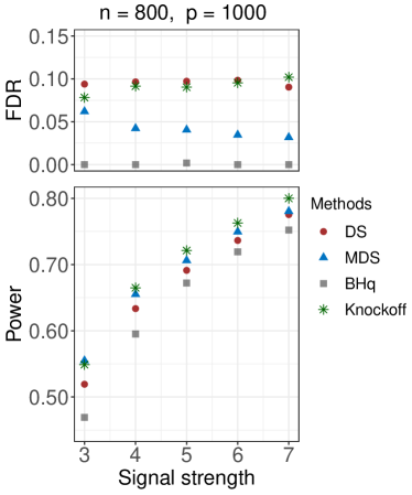
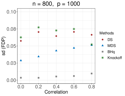
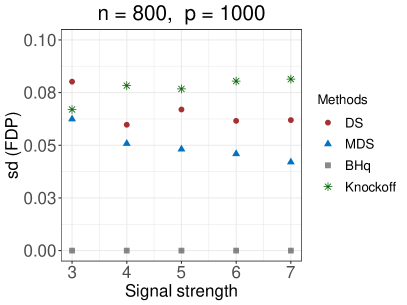
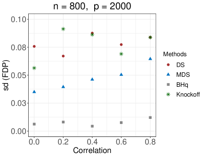
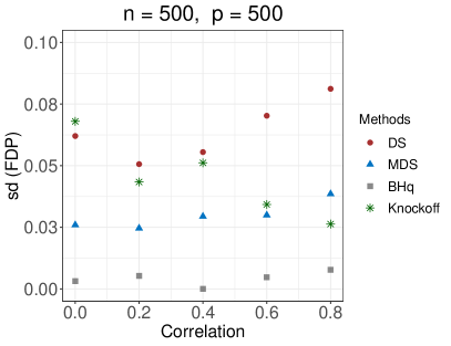
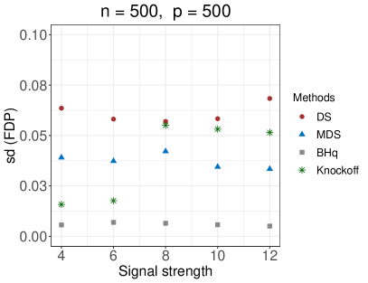
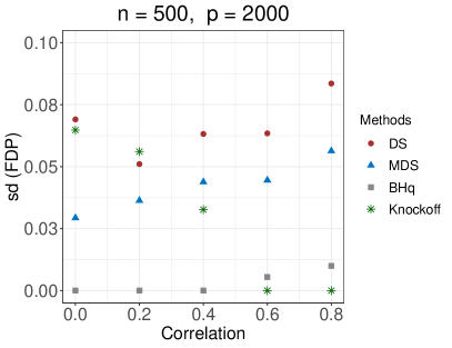
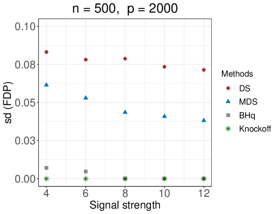
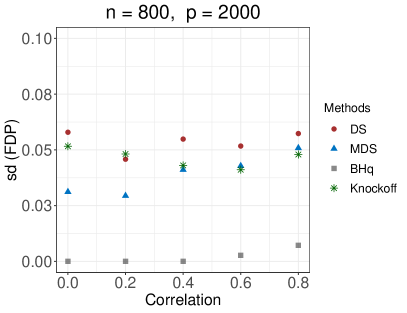
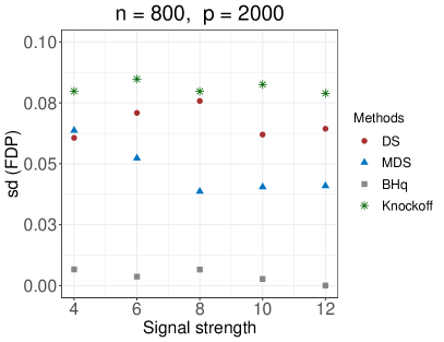
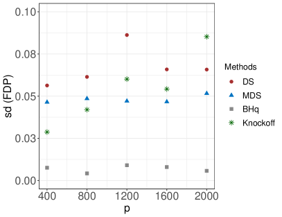
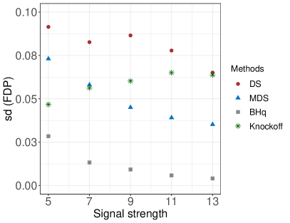
Selecting relevant features associated with a given response variable is an important issue in many scientific fields. Quantifying quality and uncertainty of a selection result via false discovery rate (FDR) control has been of recent interest. This paper introduces a way of using data-splitting strategies to asymptotically control the FDR while maintaining a high power. For each feature, the method constructs a test statistic by estimating two independent regression coefficients via data splitting. FDR control is achieved by taking advantage of the statisticโ€™s property that, for any null feature, its sampling distribution is symmetric about zero. Furthermore, we propose Multiple Data Splitting (MDS) to stabilize the selection result and boost the power. Interestingly and surprisingly, with the FDR still under control, MDS not only helps overcome the power loss caused by sample splitting, but also results in a lower variance of the false discovery proportion (FDP) compared with all other methods in consideration. We prove that the proposed data-splitting methods can asymptotically control the FDR at any designated level for linear and Gaussian graphical models in both low and high dimensions. Through intensive simulation studies and a real-data application, we show that the proposed methods are robust to the unknown distribution of features, easy to implement and computationally efficient, and are often the most powerful ones amongst competitors especially when the signals are weak and the correlations or partial correlations are high among features.

1 Introduction

1.1 Background for FDR control in regression models

Scientific researchers in the current big data era often have the privilege of collecting or accessing a large number of explanatory features targeting a specific response variable. For instance, population geneticists often need to profile thousands of single nucleotide polymorphisms (SNPs) in genome-wide association studies. A ubiquitous belief is that the response variable depends on only a small fraction of the collected features. Therefore, researchers are highly interested in identifying these relevant features so that the computability of the downstream analysis, the reproducibility of the reported results, and the interpretability of the scientific findings can be greatly enhanced. Throughout the paper, we denote the explanatory features as {X1,โ‹ฏ,Xp}subscript๐‘‹1โ‹ฏsubscript๐‘‹๐‘\{X_{1},\cdots,X_{p}\}, with p๐‘p being potentially large, and denote the response variable as y๐‘ฆy. Although the methodological developments presented here are in the context of feature selection for regression models, they can also be adapted to solve general multiple testing problems.

Many advances in feature selection methods for regression analyses have been made in the past few decades, such as stepwise regressions (Efroymson, 1960), Lasso regression (Tibshirani, 1996), and Bayesian variable selection methods (Oโ€™Hara etย al., 2009). A desired property of a selection procedure is its capability of controlling the number of false positives, which can be mathematically calibrated by the false discovery rate (FDR) (Benjamini and Hochberg, 1995) defined as follows:

FDR=๐”ผโ€‹[FDP],FDP=#โ€‹{j:jโˆˆS0,jโˆˆS^}#โ€‹{jโˆˆS^}โˆจ1,formulae-sequenceFDR๐”ผdelimited-[]FDPFDP#conditional-set๐‘—formulae-sequence๐‘—subscript๐‘†0๐‘—^๐‘†#๐‘—^๐‘†1\text{FDR}=\mathbbm{E}[\text{FDP}],\ \ \ \text{FDP}=\frac{\#\{j:j\in S_{0},\ j\in\widehat{S}\}}{\#\{j\in\widehat{S}\}\vee 1},

where S0subscript๐‘†0S_{0} denotes the index set of the null features (irrelevant features), S^^๐‘†\widehat{S} denotes the index set of the selected features, and FDP stands for โ€œfalse discovery proportionโ€. The expectation is taken with respect to the randomness in both the data and the selection procedure if it is stochastic.

One popular class of FDR control methods is based on the Benjamin-Hochberg (BHq) procedure (Benjamini and Hochberg, 1995). BHq requires p-values and guarantees exact FDR control when all the p-values are independent. Benjamini and Yekutieli (2001) generalized BHq to handle dependent p-values. They proved that BHq achieves FDR control under positive dependence, and is also valid under any arbitrary dependence structure if a shrinkage of the control level by โˆ‘j=1p1/jsuperscriptsubscript๐‘—1๐‘1๐‘—\sum_{j=1}^{p}1/j is applied. Further discussions on generalizing BHq can be found in Sarkar (2002) for general stepwise multiple testing procedures with positive dependence, Storey etย al. (2004) for weak dependence, Wu (2008) and Clarke and Hall (2009) for Markov models and linear processes.

Another class of methods is based on the โ€œknockoff filteringโ€ idea, which does not require p-values for individual features, and achieves FDR control by creating โ€œknockoffโ€ features in a similar spirit as adding spike-in controls in biological experiments. Barber and Candรจs (2015) first proposed the fixed-design knockoff filter, which achieves exact FDR control for low-dimensional Gaussian linear models regardless of the dependency structure among features. The model-X knockoff filter (Candรจs etย al., 2018) further extends the applicability of knockoff filtering to high-dimensional problems, and can be applied without having to know the underlying true relationship between the response and features. However, it requires the exact knowledge of the joint distribution of features. If this distribution is unknown, Barber etย al. (2020) showed that the inflation of the FDR is proportional to the estimation error in the conditional distribution of Xjsubscript๐‘‹๐‘—X_{j} given ๐‘ฟโˆ’jsubscript๐‘ฟ๐‘—\bm{X}_{-j}.222๐‘ฟโˆ’j={X1,โ‹ฏ,Xp}\{Xj}subscript๐‘ฟ๐‘—\subscript๐‘‹1โ‹ฏsubscript๐‘‹๐‘subscript๐‘‹๐‘—\bm{X}_{-j}=\{X_{1},\cdots,X_{p}\}\backslash\{X_{j}\}. For details on how to generate good knockoff features, see Romano etย al. (2019), Jordon etย al. (2019) (using deep generative models) and Bates etย al. (2020) (using sequential MCMC algorithms). Huang and Janson (2020) generalized the model-X knockoff filter using conditioning to allow features to follow an exponential family distribution with unknown parameters. Further developments include the multilayer knockoff filter (Katsevich and Sabatti, 2019), which achieves FDR control at both group and individual levels, and DeepPINK (Lu etย al., 2018), which models the relationship between the response and features by a neural network. Successful applications of the knockoff filter in genetics have been reported (Sesia etย al., 2018; Sesia etย al., 2020).

In this paper, we propose an FDR control framework based on data splitting. Historically, data splitting has been used for evaluating statistical predictions (e.g., cross validation) (Stone, 1974) and selecting efficient test statistics (Moran, 1973; Cox, 1975). Later, data splitting has been employed to overcome difficulties in statistical inference in high dimensions. For example, Wasserman and Roeder (2009) proposed to split the data into three parts to implement a three-stage regression method. Specifically, the user first fits a suite of candidate models to the first part of the data. The second part of the data is then used to select one of those models based on cross validations. Finally, the null features are eliminated based on hypothesis testing using the third part of the data. Other practices of data splitting in feature selection/multiple hypotheses testing can be found in Rubin etย al. (2006) (estimating the optimal cutoff for test statistics) and Ignatiadis etย al. (2016) (determining proper weights for individual hypotheses). More recently, Barber and Candรจs (2019) extended the applicability of the fixed-design knockoff filter to high-dimensional linear models via data splitting, in which the first part of the data is used to screen out enough null features so that the fixed-design knockoff filter can be applied to the selected features using the second part of the data.

FDR control originally introduced by Benjamini and Hochberg (1995) is formulated as a sampling property of the procedure, and all the aforementioned methods, including our proposed ones, take this Frequentist point of view. Bayesian views of FDR control have also been studied in the literature, such as the โ€œlocalโ€ FDR control method (Efron, 2005), which has been successfully applied to analyze microarray data (Efron etย al., 2001). The local FDR control framework is more delicate in the sense that it attaches each hypothesis/feature a probabilistic quantification of being null. However, it requires accurately estimating the densities of the test statistics, which can be challenging in practice. It is worth noting that there is also a Bayesian interpretation of the positive FDR,333The positive FDR is defined as ๐”ผ[FDPโˆฃ|S^|>0]\mathbbm{E}[\text{FDP}\mid|\widehat{S}|>0]. as pointed out by Storey (2003).

1.2 Motivations and main contributions

In high-dimensional regressions, it can be challenging to either construct valid p-values (even asymptotically) or estimate accurately the joint distribution of features, thus limiting the applicability of both BHq and the model-X knockoff filter. The data-splitting framework proposed here appears to fill in this gap. Throughout, we use DS and MDS to denote the proposed single data-splitting procedure and its refinement, the multiple data-splitting procedure, respectively. Main contributions of this work are summarized as follows.

  • โ€ข

    We propose a general FDR control framework based on data splitting, which is both conceptually simple and computationally efficient. Compared to BHq and the model-X knockoff filter, our methods require neither the p-values nor the joint distribution of features.

  • โ€ข

    We propose a general strategy to aggregate the selection results obtained from multiple independent data splits, which stabilizes the selection result and improves the power of a single data split.

  • โ€ข

    The general FDR control theories of DS and MDS are established in a model-free setting under certain assumptions, which can be further verified for the tasks of feature selection and graph estimation in linear and Gaussian graphical models under standard conditions.

  • โ€ข

    We empirically demonstrate that DS and MDS control the FDR at the designated level in all cases we have tested, and MDS achieve the best or nearly the best power in a wide range of simulation scenarios and real data applications.

DS starts by splitting the data into two halves, and then applies two potentially different statistical learning procedures to each part of the data. As mentioned in Section 1.1, the idea of using data splitting to make valid statistical inferences has been around for some time. While the main motivation of most existing methods is to handle the high-dimensionality (e.g., to obtain valid p-values or apply the fixed-design knockoff filter), we aim at obtaining two independent measurements of the importance of each feature via data splitting. FDR control is achieved by constructing a proper test statistic for each feature based on these two measurements.

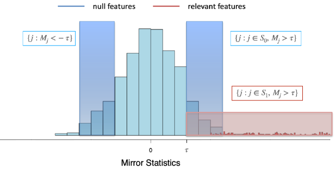
Without resorting to p-values, we follow a similar strategy as in the knockoff filter to estimate the number of false positives. The main idea is to construct a test statistic Mjsubscript๐‘€๐‘—M_{j} for each feature Xjsubscript๐‘‹๐‘—X_{j}, referred to as the โ€œmirror statisticโ€ in Xing etย al. (2019), which has the following two key properties as illustrated by Figure 1.

  1. (A1)

    A feature with a larger mirror statistic is more likely to be a relevant feature.

  2. (A2)

    The sampling distribution of the mirror statistic of any null feature is symmetric about 0.
Refer to caption
Figure 1: A cartoon illustration of the mirror statistic. Mjsubscript๐‘€๐‘—M_{j} denotes the mirror statistic of feature Xjsubscript๐‘‹๐‘—X_{j}. S0subscript๐‘†0S_{0} and S1subscript๐‘†1S_{1} denote the index set of the null features and the relevant features, respectively. Features with mirror statistics larger than the cutoff ฯ„๐œ\tau are selected.

Property (A1) suggests that we can rank the importance of each feature by its mirror statistic, and select those features with mirror statistics larger than a cutoff (ฯ„๐œ\tau in Figure 1). Property (A2) implies that we can estimate (conservatively) the number of false positives, i.e., #โ€‹{j:jโˆˆS0,Mj>ฯ„}#conditional-set๐‘—formulae-sequence๐‘—subscript๐‘†0subscript๐‘€๐‘—๐œ\#\{j:j\in S_{0},\ M_{j}>\tau\}, by #โ€‹{j:Mj<โˆ’ฯ„}#conditional-set๐‘—subscript๐‘€๐‘—๐œ\#\{j:M_{j}<-\tau\}, if the mirror statistics of the null features are not too correlated. As we will see, in our FDR control framework, Property (A1) will be naturally satisfied if the mirror statistic is properly constructed, thus our main concern is Property (A2).

MDS is built upon multiple independent replications of DS, aiming at reducing the variability of the selection result. Instead of ranking features by their mirror statistics, MDS ranks features by their inclusion rates, which are selection frequencies adjusted by selection sizes, among multiple DS replications. Empirically, we observe that MDS simultaneously reduces the FDR and boosts the power in most cases, suggesting that MDS yields better rankings of features than DS. We provide some useful insights on MDS by analyzing the simple Normal means model, in which MDS can be shown to achieve nearly the optimal detection power (see Section 2.3). MDS is conceptually most similar to the stability selection method (Meinshausen and Bรผhlmann, 2010), and a more detailed discussion about them is deferred to Section 2.2.

We specialize the applications of DS and MDS to linear and Gaussian graphical models, and show that both DS and MDS achieve FDR control under standard conditions including sparsity conditions, regularity conditions on the design matrix, and signal strength conditions. For high-dimensional linear models, we propose a Lasso + ordinary least squares (OLS) procedure. More precisely, we first screen out some null features by Lasso using one part of the data, and then run OLS on the selected features using the other part of the data. Property (A2) is satisfied if all the relevant features are selected in the first step (the so-called sure screening property). The methods designed for linear models are also applicable to Gaussian graphical models because of the linear representation of the conditional dependence structure (Lauritzen, 1996). Given a nominal level q๐‘žq, we apply DS or MDS to each nodewise regression targeting at an FDR control level q/2๐‘ž2q/2, and then combine the nodewise selection results using the OR444OR stands for โ€œorโ€, i.e., the edge (i,j)๐‘–๐‘—(i,j) is selected in the final graph if vertices Xisubscript๐‘‹๐‘–X_{i} and Xjsubscript๐‘‹๐‘—X_{j} are identified as conditional dependent in either of the nodewise regressions, Xisubscript๐‘‹๐‘–X_{i} on ๐‘ฟโˆ’isubscript๐‘ฟ๐‘–\bm{X}_{-i} or Xjsubscript๐‘‹๐‘—X_{j} on ๐‘ฟโˆ’jsubscript๐‘ฟ๐‘—\bm{X}_{-j}. See Section 3.2 for more details. rule (Meinshausen and Bรผhlmann, 2006). Numerical experiments show that DS and MDS performed significantly better than two existing methods including BHq based on the partial correlation test and the GFC555GFC stands for Gaussian graphical model estimation with false discovery rate control. method proposed in Liu (2013) specifically for handling graphical models.

The rest of the paper is structured as follows. Section 2.1 introduces DS, with a detailed discussion on the construction of the mirror statistics. Sections 2.2 and 2.3 focus on MDS, in which we show that, with high probability, the inclusion rate is a monotone decreasing function of the p-value for the Normal means model. The desired FDR control properties for DS and MDS are also established in Section 2 in a model-free setting under certain conditions. Section 3 discusses the applications of DS and MDS to linear and Gaussian graphical models. Sections 4.1 and 4.2 demonstrate the competitive performances of DS and MDS through simulation studies. Section 4.3 applies DS and MDS to the task of identifying mutations associated with drug resistance in a HIV-1 data set. Section 5 concludes with a few final remarks. We give proofs and more details on the simulation studies in Supplementary Materials.

2 Data Splitting for FDR Control

2.1 Single data splitting

Suppose a set of random features (X1,โ€ฆ,Xp)subscript๐‘‹1โ€ฆsubscript๐‘‹๐‘(X_{1},\ldots,X_{p}) follow a p๐‘p-dimensional distribution. Denote the n๐‘›n independent observations of these features as ๐‘ฟnร—p=(๐‘ฟ1,โ€ฆ,๐‘ฟp)subscript๐‘ฟ๐‘›๐‘subscript๐‘ฟ1โ€ฆsubscript๐‘ฟ๐‘\bm{X}_{n\times p}=(\bm{X}_{1},\ldots,\bm{X}_{p}), also known as the design matrix, where ๐‘ฟj=(X1โ€‹j,โ€ฆ,Xnโ€‹j)โŠบsubscript๐‘ฟ๐‘—superscriptsubscript๐‘‹1๐‘—โ€ฆsubscript๐‘‹๐‘›๐‘—โŠบ\bm{X}_{j}=(X_{1j},\ldots,X_{nj})^{\intercal} denotes the vector containing n๐‘›n independent realizations of feature Xjsubscript๐‘‹๐‘—X_{j}. We assume that each feature except the intercept with all 1โ€™s has been normalized to have zero mean and unit variance. For each set of the observed features (Xiโ€‹1,โ€ฆ,Xiโ€‹p)subscript๐‘‹๐‘–1โ€ฆsubscript๐‘‹๐‘–๐‘(X_{i1},\ldots,X_{ip}), there is an associated response variable yisubscript๐‘ฆ๐‘–y_{i} for iโˆˆ{1,โ€ฆ,n}๐‘–1โ€ฆ๐‘›i\in\{1,\ldots,n\}. Let ๐’š=(y1,โ€ฆ,yn)โŠบ๐’šsuperscriptsubscript๐‘ฆ1โ€ฆsubscript๐‘ฆ๐‘›โŠบ\bm{y}=(y_{1},\ldots,y_{n})^{\intercal} be the vector of n๐‘›n independent responses. We assume that the response variable y๐‘ฆy depends on only a subset of features XS1={Xj:jโˆˆS1}subscript๐‘‹subscript๐‘†1conditional-setsubscript๐‘‹๐‘—๐‘—subscript๐‘†1X_{S_{1}}=\{X_{j}:j\in S_{1}\}, and the task of feature selection is to identify the set S1subscript๐‘†1S_{1}. Let S0={1,โ€ฆ,p}\S1subscript๐‘†0\1โ€ฆ๐‘subscript๐‘†1S_{0}=\{1,\ldots,p\}\backslash S_{1} be the index set of the null features. Let p0=|S0|subscript๐‘0subscript๐‘†0p_{0}=|S_{0}| and p1=|S1|subscript๐‘1subscript๐‘†1p_{1}=|S_{1}| be the number of the null and the relevant features, respectively.

Feature selection commonly relies on a set of coefficients ๐œท^=(ฮฒ^1,โ‹ฏ,ฮฒ^p)โŠบ^๐œทsuperscriptsubscript^๐›ฝ1โ‹ฏsubscript^๐›ฝ๐‘โŠบ\widehat{\bm{\beta}}=(\widehat{\beta}_{1},\cdots,\widehat{\beta}_{p})^{\intercal} to measure the importance of each feature. The larger |ฮฒ^j|subscript^๐›ฝ๐‘—|\widehat{\beta}_{j}| is, the more likely feature Xjsubscript๐‘‹๐‘—X_{j} is useful in predicting y๐‘ฆy (since features have been normalized). For example, in linear regressions, ๐œท^^๐œท\widehat{\bm{\beta}} can be the vector of coefficients estimated via OLS or some shrinkage methods. In contrast to those commonly used approaches that select features based on a single set of coefficients, we construct two independent sets of coefficients, ๐œท^(1)superscriptbold-^๐œท1\bm{\widehat{\beta}}^{(1)} and ๐œท^(2)superscriptbold-^๐œท2\bm{\widehat{\beta}}^{(2)}, potentially with two different statistical procedures, in order to set up an FDR control framework. The independence between ๐œท^(1)superscriptbold-^๐œท1\bm{\widehat{\beta}}^{(1)} and ๐œท^(2)superscriptbold-^๐œท2\bm{\widehat{\beta}}^{(2)} can be ensured by employing a data-splitting strategy. More precisely, we split the n๐‘›n observations into two groups, denoted as (๐’š(1),๐‘ฟ(1))superscript๐’š1superscript๐‘ฟ1(\bm{y}^{(1)},\bm{X}^{(1)}) and (๐’š(2),๐‘ฟ(2))superscript๐’š2superscript๐‘ฟ2(\bm{y}^{(2)},\bm{X}^{(2)}). We then estimate ๐œท^(1)superscriptbold-^๐œท1\bm{\widehat{\beta}}^{(1)} based on (๐’š(1),๐‘ฟ(1))superscript๐’š1superscript๐‘ฟ1(\bm{y}^{(1)},\bm{X}^{(1)}) and ๐œท^(2)superscriptbold-^๐œท2\bm{\widehat{\beta}}^{(2)} based on (๐’š(2),๐‘ฟ(2))superscript๐’š2superscript๐‘ฟ2(\bm{y}^{(2)},\bm{X}^{(2)}). The splitting procedure is flexible, as long as the split is independent of the response vector ๐’š๐’š\bm{y}. The sample sizes for the two groups can also be potentially different. Empirically, we find that the half-half sample splitting leads to the highest power. To achieve FDR control under our data-splitting framework, the two sets of coefficients shall satisfy the following assumption besides being independent.

Assumption 1

(Symmetry) For each null feature index jโˆˆS0๐‘—subscript๐‘†0j\in S_{0}, the sampling distribution of either ฮฒ^j(1)subscriptsuperscript^๐›ฝ1๐‘—\widehat{\beta}^{(1)}_{j} or ฮฒ^j(2)subscriptsuperscript^๐›ฝ2๐‘—\widehat{\beta}^{(2)}_{j} is symmetric about 0.

Note that the symmetry assumption is only required for the null features and can be further relaxed to asymptotic symmetry. Furthermore, for jโˆˆS0๐‘—subscript๐‘†0j\in S_{0}, it is sufficient that only one of ฮฒ^j(1)subscriptsuperscript^๐›ฝ1๐‘—\widehat{\beta}^{(1)}_{j} and ฮฒ^j(2)subscriptsuperscript^๐›ฝ2๐‘—\widehat{\beta}^{(2)}_{j} is symmetric about 0. In Section 3, we propose a Lasso + OLS procedure for linear and Gaussian graphical models so that the symmetry assumption can be satisfied with probability approaching 1 under certain conditions.

Our FDR control framework starts with the construction of a mirror statistic that satisfies Properties (A1) and (A2) as discussed in Section 1.2. A general form of the mirror statistic Mjsubscript๐‘€๐‘—M_{j} is

Mj=signโ€‹(ฮฒ^j(1)โ€‹ฮฒ^j(2))โ€‹fโ€‹(|ฮฒ^j(1)|,|ฮฒ^j(2)|),subscript๐‘€๐‘—signsuperscriptsubscript^๐›ฝ๐‘—1superscriptsubscript^๐›ฝ๐‘—2๐‘“superscriptsubscript^๐›ฝ๐‘—1superscriptsubscript^๐›ฝ๐‘—2M_{j}=\text{sign}\big{(}\widehat{\beta}_{j}^{(1)}\widehat{\beta}_{j}^{(2)}\big{)}f\big{(}|\widehat{\beta}_{j}^{(1)}|,|\widehat{\beta}_{j}^{(2)}|\big{)}, (1)

where function fโ€‹(u,v)๐‘“๐‘ข๐‘ฃf(u,v) is non-negative, symmetric about u๐‘ขu and v๐‘ฃv, and monotonically increasing in both u๐‘ขu and v๐‘ฃv. For a relevant feature, the two coefficients tend to be large (in the absolute value) and have the same sign if the estimation procedures are reasonably efficient. Since fโ€‹(u,v)๐‘“๐‘ข๐‘ฃf(u,v) is monotonically increasing in both u๐‘ขu and v๐‘ฃv, the corresponding mirror statistic is likely to be positive and relatively large, which implies Property (A1). In addition, the independence between the two coefficients, together with the symmetry assumption, imply Property (A2) as shown by Lemma 1.

Lemma 1

Under Assumption 1, regardless of the data-splitting procedure, the sampling distribution of Mjsubscript๐‘€๐‘—M_{j} is symmetric about 0 for jโˆˆS0๐‘—subscript๐‘†0j\in S_{0}.

The proof is elementary and thus omitted. Three convenient choices of fโ€‹(u,v)๐‘“๐‘ข๐‘ฃf(u,v) are:

fโ€‹(u,v)=2โ€‹minโก(u,v),fโ€‹(u,v)=uโ€‹v,fโ€‹(u,v)=u+v.formulae-sequence๐‘“๐‘ข๐‘ฃ2๐‘ข๐‘ฃformulae-sequence๐‘“๐‘ข๐‘ฃ๐‘ข๐‘ฃ๐‘“๐‘ข๐‘ฃ๐‘ข๐‘ฃf(u,v)=2\min(u,v),\ \ \ f(u,v)=uv,\ \ \ f(u,v)=u+v. (2)

The first choice equals to the mirror statistic proposed in Xing etย al. (2019), and the third choice corresponds to the โ€œsign-maximumโ€ between |ฮฒ^j(1)+ฮฒ^j(2)|superscriptsubscript^๐›ฝ๐‘—1superscriptsubscript^๐›ฝ๐‘—2\big{|}\widehat{\beta}_{j}^{(1)}+\widehat{\beta}_{j}^{(2)}\big{|} and |ฮฒ^j(1)โˆ’ฮฒ^j(2)|superscriptsubscript^๐›ฝ๐‘—1superscriptsubscript^๐›ฝ๐‘—2\big{|}\widehat{\beta}_{j}^{(1)}-\widehat{\beta}_{j}^{(2)}\big{|}, and is optimal in a simplified setting as described in Proposition 1. The optimally of the sign-max mirror statistic has also been empirically observed by Barber and Candรจs (2015), and been recently proved by Ke etย al. (2020) based on a more delicate analysis under the weak-and-rare signal setting.

Proposition 1

Suppose the set of coefficients (ฮฒ^j(1),ฮฒ^j(2))superscriptsubscript^๐›ฝ๐‘—1superscriptsubscript^๐›ฝ๐‘—2(\widehat{\beta}_{j}^{(1)},\widehat{\beta}_{j}^{(2)}) are independent over the feature index jโˆˆ{1,โ€ฆ,p}๐‘—1โ€ฆ๐‘j\in\{1,\ldots,p\}. Furthermore, suppose (a) for jโˆˆS0๐‘—subscript๐‘†0j\in S_{0}, the two coefficients ฮฒ^j(1)superscriptsubscript^๐›ฝ๐‘—1\widehat{\beta}_{j}^{(1)} and ฮฒ^j(2)superscriptsubscript^๐›ฝ๐‘—2\widehat{\beta}_{j}^{(2)} follow Nโ€‹(0,1)๐‘01N(0,1) independently; (b) for jโˆˆS1๐‘—subscript๐‘†1j\in S_{1}, the two coefficients follow Nโ€‹(ฯ‰,1)๐‘๐œ”1N(\omega,1) independently; and (c) p1/p0โ†’rโ†’subscript๐‘1subscript๐‘0๐‘Ÿp_{1}/p_{0}{\rightarrow}r as pโ†’โˆžโ†’๐‘p\to\infty. Then, fโ€‹(u,v)=u+v๐‘“๐‘ข๐‘ฃ๐‘ข๐‘ฃf(u,v)=u+v is the optimal choice that yields the highest power.

Proposition 1 still holds if the set of coefficients (ฮฒ^j(1),ฮฒ^j(2))superscriptsubscript^๐›ฝ๐‘—1superscriptsubscript^๐›ฝ๐‘—2(\widehat{\beta}_{j}^{(1)},\widehat{\beta}_{j}^{(2)}) are only weakly correlated over the feature index j๐‘—j, as long as the following law of large numbers is satisfied:

limpโ†’โˆž#โ€‹{j:jโˆˆS0,jโˆˆS^}#โ€‹{j:jโˆˆS^}=โ„™โ€‹(jโˆˆS^โˆฃjโˆˆS0)โ„™โ€‹(jโˆˆS^โˆฃjโˆˆS0)+rโ€‹โ„™โ€‹(jโˆˆS^โˆฃjโˆˆS1).subscriptโ†’๐‘#conditional-set๐‘—formulae-sequence๐‘—subscript๐‘†0๐‘—^๐‘†#conditional-set๐‘—๐‘—^๐‘†โ„™๐‘—conditional^๐‘†๐‘—subscript๐‘†0โ„™๐‘—conditional^๐‘†๐‘—subscript๐‘†0๐‘Ÿโ„™๐‘—conditional^๐‘†๐‘—subscript๐‘†1\lim_{p\to\infty}\frac{\#\{j:j\in S_{0},j\in\widehat{S}\}}{\#\{j:j\in\widehat{S}\}}=\frac{\mathbbm{P}(j\in\widehat{S}\mid j\in S_{0})}{\mathbbm{P}(j\in\widehat{S}\mid j\in S_{0})+r\mathbbm{P}(j\in\widehat{S}\mid j\in S_{1})}.

The proof of Proposition 1 (see Supplementary Materials) might be of general interest. We rephrase the FDR control problem under the hypothesis testing framework, and prove the optimality using the Neyman-Pearson lemma. The form fโ€‹(u,v)=u+v๐‘“๐‘ข๐‘ฃ๐‘ข๐‘ฃf(u,v)=u+v is derived based on the rejection rule of the corresponding likelihood ratio test. For linear models in more realistic settings, we empirically compare the performances of the three choices of fโ€‹(u,v)๐‘“๐‘ข๐‘ฃf(u,v) listed in (2) in Section 4.1.

The symmetric property of the mirror statistics for the null features gives us an upper bound of the number of false positives:

#โ€‹{jโˆˆS0:Mj>t}โ‰ˆ#โ€‹{jโˆˆS0:Mj<โˆ’t}โ‰ค#โ€‹{j:Mj<โˆ’t},โˆ€t>0.formulae-sequence#conditional-set๐‘—subscript๐‘†0subscript๐‘€๐‘—๐‘ก#conditional-set๐‘—subscript๐‘†0subscript๐‘€๐‘—๐‘ก#conditional-set๐‘—subscript๐‘€๐‘—๐‘กfor-all๐‘ก0\#\{j\in S_{0}:M_{j}>t\}\approx\#\{j\in S_{0}:M_{j}<-t\}\leq\#\{j:M_{j}<-t\},\ \ \ \forall\ t>0. (3)

The FDPโ€‹(t)FDP๐‘ก\text{FDP}(t) of the selection S^t={j:Mj>t}subscript^๐‘†๐‘กconditional-set๐‘—subscript๐‘€๐‘—๐‘ก\widehat{S}_{t}=\{j:M_{j}>t\}, as well as an โ€œover estimateโ€ of it, referred to as FDP^โ€‹(t)^FDP๐‘ก\widehat{\text{FDP}}(t) in the following, are thus given by

FDPโ€‹(t)=#โ€‹{j:Mj>t,jโˆˆS0}#โ€‹{j:Mj>t}โˆจ1,FDP^โ€‹(t)=#โ€‹{j:Mj<โˆ’t}#โ€‹{j:Mj>t}โˆจ1.formulae-sequenceFDP๐‘ก#conditional-set๐‘—formulae-sequencesubscript๐‘€๐‘—๐‘ก๐‘—subscript๐‘†0#conditional-set๐‘—subscript๐‘€๐‘—๐‘ก1^FDP๐‘ก#conditional-set๐‘—subscript๐‘€๐‘—๐‘ก#conditional-set๐‘—subscript๐‘€๐‘—๐‘ก1\text{FDP}(t)=\frac{\#\{j:M_{j}>t,\ j\in S_{0}\}}{\#\{j:M_{j}>t\}\vee 1},\ \ \ \ \ \ \widehat{\text{FDP}}(t)=\frac{\#\{j:M_{j}<-t\}}{\#\{j:M_{j}>t\}\vee 1}.

For any designated FDR control level qโˆˆ(0,1)๐‘ž01q\in(0,1), we can choose the data-driven cutoff ฯ„qsubscript๐œ๐‘ž\tau_{q} as follows:

ฯ„q=minโก{t>0:FDP^โ€‹(t)โ‰คq},subscript๐œ๐‘ž:๐‘ก0^FDP๐‘ก๐‘ž\tau_{q}=\min\{t>0:\widehat{\text{FDP}}(t)\leq q\},

and the final selection is S^ฯ„q={j:Mj>ฯ„q}subscript^๐‘†subscript๐œ๐‘žconditional-set๐‘—subscript๐‘€๐‘—subscript๐œ๐‘ž\widehat{S}_{\tau_{q}}=\{j:M_{j}>\tau_{q}\}. The proposed FDR control procedure is summarized in Algorithm 1.

Algorithm 1 False discovery rate control via a single data split
  1. 1.

    Split the data into two groups (๐’š(1),๐‘ฟ(1))superscript๐’š1superscript๐‘ฟ1(\bm{y}^{(1)},\bm{X}^{(1)}) and (๐’š(2),๐‘ฟ(2))superscript๐’š2superscript๐‘ฟ2(\bm{y}^{(2)},\bm{X}^{(2)}), independent to the response vector ๐’š๐’š\bm{y}.

  2. 2.

    Estimate the โ€œimpactโ€ coefficients ๐œท^(1)superscriptbold-^๐œท1\bm{\widehat{\beta}}^{(1)} and ๐œท^(2)superscriptbold-^๐œท2\bm{\widehat{\beta}}^{(2)} on each part of the data. The two estimation procedures can be potentially different.

  3. 3.

    Calculate the mirror statistics following (1).

  4. 4.

    Given a designated FDR level qโˆˆ(0,1)๐‘ž01q\in(0,1), calculate the cutoff ฯ„qsubscript๐œ๐‘ž\tau_{q} as:

    ฯ„q=minโก{t>0:FDP^โ€‹(t)=#โ€‹{j:Mj<โˆ’t}#โ€‹{j:Mj>t}โˆจ1โ‰คq}.subscript๐œ๐‘ž:๐‘ก0^FDP๐‘ก#conditional-set๐‘—subscript๐‘€๐‘—๐‘ก#conditional-set๐‘—subscript๐‘€๐‘—๐‘ก1๐‘ž\tau_{q}=\min\left\{t>0:\widehat{\text{FDP}}(t)=\frac{\#\{j:M_{j}<-t\}}{\#\{j:M_{j}>t\}\vee 1}\leq q\right\}. (4)
  5. 5.

    Select the features {j:Mj>ฯ„q}conditional-set๐‘—subscript๐‘€๐‘—subscript๐œ๐‘ž\{j:M_{j}>\tau_{q}\}.

In order to obtain a good estimate of the number of false positives using (3), the mirror statistics of the null features cannot be too correlated. Mathematically, we require the following weak dependence assumption.

Assumption 2

(Weak dependence among the null features) The mirror statistics Mjโ€ฒโ€‹ssuperscriptsubscript๐‘€๐‘—โ€ฒ๐‘ M_{j}^{\prime}s are continuous random variables, and there exist constants c>0๐‘0c>0 and ฮฑโˆˆ(0,2)๐›ผ02\alpha\in(0,2) such that

Varโ€‹(โˆ‘jโˆˆS0๐Ÿ™โ€‹(Mj>t))โ‰คcโ€‹p0ฮฑ,โˆ€tโˆˆโ„,whereย โ€‹p0=|S0|.formulae-sequenceVarsubscript๐‘—subscript๐‘†01subscript๐‘€๐‘—๐‘ก๐‘superscriptsubscript๐‘0๐›ผformulae-sequencefor-all๐‘กโ„whereย subscript๐‘0subscript๐‘†0\textnormal{Var}\bigg{(}\sum_{j\in S_{0}}\mathbbm{1}(M_{j}>t)\bigg{)}\leq cp_{0}^{\alpha},\ \ \forall\ t\in\mathbbm{R},\ \ \mbox{where }p_{0}=|S_{0}|.

Assumption 2 only restricts the correlations among the null features, regardless of the correlations associated with the relevant features. We note that if the mirror statistics of the null features have constant pairwise correlations, or can be clustered into a fixed number of groups (say, 2) so that their within-group correlation is a constant, ฮฑ๐›ผ\alpha has to be 2 and Assumption 2 does not hold. Except for these extreme cases, we believe that Assumption 2 holds in fairly broad settings. For example, in Section 3.1, we show that for linear models, the weak dependence assumption holds as long as the covariance matrix of the null features satisfies some regularity condition (e.g., the eigenvalues are doubly bounded). Empirically, we observed that even in the case where the null features have constant pairwise correlations, our methods still perform very well, often outperforming BHq and the knockoff filters (see Figure 19 in Supplementary Materials).

Recall that FDPโ€‹(t)FDP๐‘ก\text{FDP}(t) refers to the FDP of the selection S^t={j:Mj>t}subscript^๐‘†๐‘กconditional-set๐‘—subscript๐‘€๐‘—๐‘ก\widehat{S}_{t}=\{j:M_{j}>t\}. We assume that the variances of the mirror statistics do not diverge to infinity and are also bounded away from 0. The proposition below shows that for any nominal level qโˆˆ(0,1)๐‘ž01q\in(0,1), FDPโ€‹(ฯ„q)FDPsubscript๐œ๐‘ž\text{FDP}(\tau_{q}) and the corresponding FDRโ€‹(ฯ„q)FDRsubscript๐œ๐‘ž\text{FDR}(\tau_{q}) are under control, in which ฯ„qsubscript๐œ๐‘ž\tau_{q} is the data-dependent cutoff chosen following (4).

Proposition 2

For any designated FDR control level qโˆˆ(0,1)๐‘ž01q\in(0,1), assume that there exists a constant tq>0subscript๐‘ก๐‘ž0t_{q}>0 such that โ„™โ€‹(FDPโ€‹(tq)โ‰คq)โ†’1โ†’โ„™FDPsubscript๐‘ก๐‘ž๐‘ž1\mathbbm{P}(\text{FDP}(t_{q})\leq q)\to 1 as pโ†’โˆžโ†’๐‘p\to\infty. Then, under Assumptions 1 and 2, the procedure in Algorithmย 1 satisfies

FDPโ€‹(ฯ„q)โ‰คq+opโ€‹(1)andlim suppโ†’โˆžFDRโ€‹(ฯ„q)โ‰คq.formulae-sequenceFDPsubscript๐œ๐‘ž๐‘žsubscript๐‘œ๐‘1andsubscriptlimit-supremumโ†’๐‘FDRsubscript๐œ๐‘ž๐‘ž\text{FDP}(\tau_{q})\leq q+o_{p}(1)\ \ \ \text{and}\ \ \ \limsup_{p\to\infty}\text{FDR}(\tau_{q})\leq q.

We note that the existence of tq>0subscript๐‘ก๐‘ž0t_{q}>0 such that โ„™โ€‹(FDPโ€‹(tq)โ‰คq)โ†’1โ†’โ„™FDPsubscript๐‘ก๐‘ž๐‘ž1\mathbbm{P}(\text{FDP}(t_{q})\leq q)\to 1 essentially guarantees the asymptotic feasibility of FDR control based upon the rankings of features by their mirror statistics. Specifically, it implies that the data-dependent cutoff ฯ„qsubscript๐œ๐‘ž\tau_{q} is bounded with probability approaching 1, thus does not diverge to infinity. It is a technical assumption for handling the most general setting without specifying a parametric model between the response and features. When we work with specific models such as linear or Gaussian graphical models, this technical assumption is no longer required (see Section 3.1). Similar assumptions also appear in Storey etย al. (2004) and Wu (2008) in order to achieve a high level of generality.

In Assumption 1, the exact symmetry can be relaxed to asymptotic symmetry. Suppose for jโˆˆS0๐‘—subscript๐‘†0j\in S_{0}, the sampling distribution of either ฮฒ^j(1)subscriptsuperscript^๐›ฝ1๐‘—\widehat{\beta}^{(1)}_{j} or ฮฒ^j(2)subscriptsuperscript^๐›ฝ2๐‘—\widehat{\beta}^{(2)}_{j} is asymptotically symmetric about 0. In addition, the asymptotic symmetry is uniform over jโˆˆS0๐‘—subscript๐‘†0j\in S_{0} in the sense that the resulting mirror statistics satisfy the following condition,

maxjโˆˆS0โก|โ„™โ€‹(Mj>t)โˆ’โ„™โ€‹(Mj<โˆ’t)|โ†’0,โˆ€t.โ†’subscript๐‘—subscript๐‘†0โ„™subscript๐‘€๐‘—๐‘กโ„™subscript๐‘€๐‘—๐‘ก0for-all๐‘ก\max_{j\in S_{0}}\left|\mathbbm{P}(M_{j}>t)-\mathbbm{P}(M_{j}<-t)\right|\to 0,\ \ \ \forall\ t.

Then Proposition 2 still holds. As for high-dimensional generalized linear models, one way to construct the mirror statistic is to use the debiased Lasso estimator (Van de Geer etย al., 2014; Zhang and Zhang, 2014; Javanmard and Montanari, 2014), which is asymptotically normal, and therefore symmetric. Furthermore, under certain conditions, the bias in the debiased Lasso estimator vanishes uniformly over the features. Thus, the proposed methodologies are applicable, and we refer the readers to Dai etย al. (2020) for more details.

Before concluding this section, we remark that DS is inspired by the recently proposed Gaussian mirror method (Xing etย al., 2019), which perturbs the features one by one and examines the corresponding impact. Compared to the Gaussian mirror method, DS is easier to implement and computationally more efficient especially for large n๐‘›n and p๐‘p. For linear models, the Gaussian mirror method requires p๐‘p linear fittings. In contrast, DS perturbs all the features simultaneously by randomly splitting the data into two halves, thus requiring only two linear fittings. The gain of the computational efficiency can be more significant for Gaussian graphical models (see Section 3.2). DS requires 2โ€‹p2๐‘2p nodewise linear fittings, whereas the Gaussian mirror method would require p2superscript๐‘2p^{2} nodewise linear fittings, which is generally unacceptable when p๐‘p is large. In addition, since DS is conceptually simpler, it is more convenient to adapt DS to other statistical models.

2.2 Multiple data splitting

There are two major concerns about DS. First, splitting the data into two halves inflates the variances of the estimated regression coefficients, thus DS can potentially suffer a power loss in comparison with competing methods that properly use the full data. Second, the selection result of DS may not be stable and can vary substantially across different sample splits.

To remedy these issues, we propose a multiple data-splitting (MDS) procedure to aggregate the selection results obtained from independent replications of DS. For linear and Gaussian graphical models, we prove that MDS achieves FDR control under certain conditions. Simulation results in Section 4 confirm FDR control of MDS and demonstrate a fairly universal power improvement of MDS over DS. Going beyond these two models, we empirically found that MDS can work competitively for a much wider class of models. MDS is also generally applicable without requiring p-values or any knowledge regarding the joint distribution of features.

Given (๐‘ฟ,๐’š)๐‘ฟ๐’š(\bm{X},\bm{y}), suppose we independently repeat DS m๐‘šm times with random sample splits. Each time the set of selected features is denoted as S^(k)superscript^๐‘†๐‘˜\widehat{S}^{(k)} for k=1,โ€ฆ,m๐‘˜1โ€ฆ๐‘šk=1,\ldots,m. For each feature Xjsubscript๐‘‹๐‘—X_{j}, we define the associated inclusion rate Ijsubscript๐ผ๐‘—I_{j} and its estimate I^jsubscript^๐ผ๐‘—\widehat{I}_{j} as

Ij=๐”ผ[๐Ÿ™โ€‹(jโˆˆS^)|S^|โˆจ1|๐‘ฟ,๐’š],I^j=1mโˆ‘k=1m๐Ÿ™โ€‹(jโˆˆS^(k))|S^(k)|โˆจ1,I_{j}=\mathbbm{E}\left[\frac{\mathbbm{1}(j\in\widehat{S})}{|\widehat{S}|\vee 1}\biggm{|}\bm{X},\bm{y}\right],\ \ \ \widehat{I}_{j}=\frac{1}{m}\sum_{k=1}^{m}\frac{\mathbbm{1}(j\in\widehat{S}^{(k)})}{|\widehat{S}^{(k)}|\vee 1}, (5)

in which the expectation is taken with respect to the randomness in data splitting. Note that this rate is not an estimate of the selection probability, but rather an importance measurement of each feature relative to the DS selection procedure. For example, in the case where feature Xjsubscript๐‘‹๐‘—X_{j} is always selected by DS and DS always selects 20 features across m๐‘šm random sample splits, the inclusion rate Ijsubscript๐ผ๐‘—I_{j} equals to 1/20. MDS is most useful if the following informal statement is approximately true: if a feature is selected less frequently in the repeated sample splitting, it is less likely to be a relevant feature. In other words, the rankings of features by the inclusion rates should roughly reflect the importance of features. If this holds, we can choose a proper inclusion-rate cutoff to control the FDR, and select those features with inclusion rates larger than the cutoff.

The way of choosing a proper inclusion-rate cutoff is detailed in Algorithm 2 and briefly discussed here. Let the sorted inclusion rate estimates be 0โ‰คI^(1)โ‰คI^(2)โ‰คโ‹ฏโ‰คI^(p)0subscript^๐ผ1subscript^๐ผ2โ‹ฏsubscript^๐ผ๐‘0\leq\widehat{I}_{(1)}\leq\widehat{I}_{(2)}\leq\cdots\leq\widehat{I}_{(p)}. Proposition 2 suggests a backtracking approach to select the cutoff based on the following argument: if we had m๐‘šm independent sets of data (๐‘ฟ,๐’š)๐‘ฟ๐’š(\bm{X},\bm{y}) and applied DS to all of them for feature selection, the average FDP would be (asymptotically) no larger than the designated FDR control level q๐‘žq. Although it is not possible to generate new data, we can consider {S^(k),k=1,โ€ฆ,m}formulae-sequencesuperscript^๐‘†๐‘˜๐‘˜1โ€ฆ๐‘š\{\widehat{S}^{(k)},\ k=1,\ldots,m\} as an approximation to m๐‘šm independent selection results obtained via data regeneration. We thus find the largest cutoff such that, if we assume that the features with inclusion rates larger/smaller than the cutoff are โ€œtrueโ€ relevant/null features, respectively, the average FDP among {S^(k),k=1,โ€ฆ,m}formulae-sequencesuperscript^๐‘†๐‘˜๐‘˜1โ€ฆ๐‘š\{\widehat{S}^{(k)},\ k=1,\ldots,m\} is no larger than q๐‘žq. Empirically, we find that MDS often results in a lower FDR than the nominal level but still enjoys a competitive power. The proposition below gives some intuitions regarding how MDS is guaranteed to control the FDR properly.

Algorithm 2 Aggregating selection results from multiple data splits.
  1. 1.

    Sort the estimated inclusion rates (see (5)): 0โ‰คI^(1)โ‰คI^(2)โ‰คโ‹ฏโ‰คI^(p)0subscript^๐ผ1subscript^๐ผ2โ‹ฏsubscript^๐ผ๐‘0\leq\widehat{I}_{(1)}\leq\widehat{I}_{(2)}\leq\cdots\leq\widehat{I}_{(p)}.

  2. 2.

    Find the largest โ„“โˆˆ{1,โ€ฆ,p}โ„“1โ€ฆ๐‘\ell\in\{1,\ldots,p\} such that I^(1)+โ‹ฏ+I^(โ„“)โ‰คqsubscript^๐ผ1โ‹ฏsubscript^๐ผโ„“๐‘ž\widehat{I}_{(1)}+\cdots+\widehat{I}_{(\ell)}\leq q.

  3. 3.

    Select the features S^={j:I^j>I^(โ„“)}^๐‘†conditional-set๐‘—subscript^๐ผ๐‘—subscript^๐ผโ„“\widehat{S}=\{j:\widehat{I}_{j}>\widehat{I}_{(\ell)}\}.

Proposition 3

Suppose we can asymptotically control the FDP of DS for any designated level qโˆˆ(0,1)๐‘ž01q\in(0,1).666In the sparse regime, we shall asymptotically control the FDP of DS at some level qโ€ฒ<qsuperscript๐‘žโ€ฒ๐‘žq^{\prime}<q in order to bypass the technical difficulties. Since qโ€ฒsuperscript๐‘žโ€ฒq^{\prime} can be arbitrarily close to q๐‘žq, this modification is purely for the technical purpose and has almost no practical implications. Furthermore, we assume that with probability approaching 1, the power of DS is bounded below by some ฮบ>0๐œ…0\kappa>0. We consider the following two regimes with n,pโ†’โˆžโ†’๐‘›๐‘n,p\to\infty at a proper rate.

  1. (a)

    In the non-sparse regime where lim infp1/p>0limit-infimumsubscript๐‘1๐‘0\liminf p_{1}/p>0, we assume that the mirror statistics are consistent at ranking features, i.e., supiโˆˆS1,jโˆˆS0โ„™โ€‹(Ii<Ij)โ†’0โ†’subscriptsupremumformulae-sequence๐‘–subscript๐‘†1๐‘—subscript๐‘†0โ„™subscript๐ผ๐‘–subscript๐ผ๐‘—0\sup_{i\in S_{1},j\in S_{0}}\mathbbm{P}(I_{i}<I_{j})\to 0.

  2. (b)

    In the sparse regime where lim supp1/p=0limit-supremumsubscript๐‘1๐‘0\limsup p_{1}/p=0, we assume that the mirror statistics are strongly consistent at ranking features, i.e., supiโˆˆS1โ„™โ€‹(Ii<maxjโˆˆS0โกIj)โ†’0โ†’subscriptsupremum๐‘–subscript๐‘†1โ„™subscript๐ผ๐‘–subscript๐‘—subscript๐‘†0subscript๐ผ๐‘—0\sup_{i\in S_{1}}\mathbbm{P}(I_{i}<\max_{j\in S_{0}}I_{j})\to 0.

Then, for MDS (see Algorithm 2) in both the non-sparse and the sparse regimes, we have

FDPโ‰คq+opโ€‹(1)andlim supn,pโ†’โˆžFDRโ‰คq.formulae-sequenceFDP๐‘žsubscript๐‘œ๐‘1andsubscriptlimit-supremumโ†’๐‘›๐‘FDR๐‘ž\text{FDP}\leq q+o_{p}(1)\ \ \ \text{and}\ \ \ \limsup_{n,p\to\infty}\text{FDR}\leq q.

Although some of the conditions in Proposition 3 are not explicit enough or directly verifiable without imposing a specific model and the associated assumptions, the proposition points out a key factor for MDS to achieve FDR control: the ranking consistency of the baseline algorithm. More precisely, assuming that the mirror statistics are consistent at ranking features (see Proposition 3(a)), we can show that the number of false positives is in the order of opโ€‹(p0)subscript๐‘œ๐‘subscript๐‘0o_{p}(p_{0}). In the non-sparse regime, this leads to the desired FDR control property for MDS as p1subscript๐‘1p_{1} and p0subscript๐‘0p_{0} are in the same order. In the sparse regime, since p0โ‰ซp1much-greater-thansubscript๐‘0subscript๐‘1p_{0}\gg p_{1}, we require a stronger ranking consistency condition (see Proposition 3(b)), under which we can show that the number of false positives is in the order of opโ€‹(p1)subscript๐‘œ๐‘subscript๐‘1o_{p}(p_{1}). In Section 3, we show that the ranking consistency condition holds for linear and Gaussian graphical models under more explicit conditions.

The idea of using data perturbation and replicating the procedure multiple times to stabilize the selection results is not new. For example, Meinshausen and Bรผhlmann (2010) proposed a stability selection method, which perturbs the data via subsampling and runs a feature selection algorithm multiple times across a set of regularization parameters. The final selection set only contains โ€œstableโ€ features, of which the selection frequencies under different magnitudes of regularization are above some user-defined threshold. Compared with the stability selection method, the motivation of MDS is different. The stability selection method aims at overcoming the difficulty of finding a proper regularization parameter in high-dimensional regression, whereas MDS is designed to stabilize DS and compensate for its power loss due to sample splitting. Theoretically, under certain conditions, the stability selection method provides some finite-sample bound on the number of false positives, whereas MDS asymptotically controls the perhaps more delicate FDR. Indeed, MDS requires a careful selection of the inclusion-rate cutoff in order to achieve FDR control. In contrast, for the stability selection method, the corresponding selection-probability cutoff can be much less stringent. Furthermore, the two methods perturb the data in different ways. For each regularization parameter, the stability selection method obtains a collection of selection sets using different sub-samples of the data, whereas MDS always uses the full data, but replicates DS with independent sample splits so as to obtain multiple selection results.

There are also some relevant works on p-value aggregation in high-dimensional settings. For example, Meinshausen etย al. (2009) proposed to obtain a collection of p-values via repeated sample splitting. The multiple p-values of each feature are then aggregated by choosing a proper quantile among them. After that, BHq can be applied to control the FDR. Empirically, we found that the resulting procedure is often too conservative, with a near-zero FDR but also a sub-optimal power (see Section 4.1). For other related works, we refer the readers to vanย de Wiel etย al. (2009) and Romano and DiCiccio (2019).

2.3 A theoretical study of MDS for the Normal means model

We consider the simple Normal means model to gain some insights on how MDS compensates for the power loss of DS due to sample splitting. For i=1,โ€ฆ,n๐‘–1โ€ฆ๐‘›i=1,\ldots,n and j=1,โ€ฆ,p๐‘—1โ€ฆ๐‘j=1,\ldots,p, we assume that Xiโ€‹jsubscript๐‘‹๐‘–๐‘—X_{ij} follows Nโ€‹(ฮผj,1)๐‘subscript๐œ‡๐‘—1N(\mu_{j},1) independently. To test whether ฮผjsubscript๐œ‡๐‘—\mu_{j} is 0, the p-value is given by pj=2โ€‹ฮฆโ€‹(โˆ’|nโ€‹๐‘ฟjยฏ|)subscript๐‘๐‘—2ฮฆ๐‘›ยฏsubscript๐‘ฟ๐‘—p_{j}=2\Phi(-|\sqrt{n}\bar{\bm{X}_{j}}|), where ๐‘ฟยฏj=โˆ‘i=1nXiโ€‹j/nsubscriptยฏ๐‘ฟ๐‘—superscriptsubscript๐‘–1๐‘›subscript๐‘‹๐‘–๐‘—๐‘›\bar{\bm{X}}_{j}=\sum_{i=1}^{n}X_{ij}/n, and ฮฆฮฆ\Phi is the CDF of the standard Normal distribution.

For DS, we construct the mirror statistic Mjsubscript๐‘€๐‘—M_{j} using the sample means of ๐‘ฟj(1)superscriptsubscript๐‘ฟ๐‘—1\bm{X}_{j}^{(1)} and ๐‘ฟj(2)superscriptsubscript๐‘ฟ๐‘—2\bm{X}_{j}^{(2)}, and select S^^๐‘†\widehat{S}, i.e., reject the null hypotheses that ฮผjsubscript๐œ‡๐‘—\mu_{j}โ€™s are 0, following Algorithm 1. For MDS, we replicate DS m๐‘šm times and estimate the inclusion rates following (5). Proposition 4 below holds for any designated FDR control level qโˆˆ(0,1)๐‘ž01q\in(0,1), and for all three choices of f๐‘“f detailed in (2) for constructing the mirror statistics. For simplicity, we only prove the case for

Mj=|๐‘ฟยฏj(1)+๐‘ฟยฏj(2)|โˆ’|๐‘ฟยฏj(1)โˆ’๐‘ฟยฏj(2)|.subscript๐‘€๐‘—superscriptsubscriptยฏ๐‘ฟ๐‘—1superscriptsubscriptยฏ๐‘ฟ๐‘—2superscriptsubscriptยฏ๐‘ฟ๐‘—1superscriptsubscriptยฏ๐‘ฟ๐‘—2M_{j}=|\bar{\bm{X}}_{j}^{(1)}+\bar{\bm{X}}_{j}^{(2)}|-|\bar{\bm{X}}_{j}^{(1)}-\bar{\bm{X}}_{j}^{(2)}|. (6)
Proposition 4

For any pair (i,j)๐‘–๐‘—(i,j) and two arbitrary constants 0<c<cโ€ฒ0๐‘superscript๐‘โ€ฒ0<c<c^{\prime}, as nโ†’โˆžโ†’๐‘›n\to\infty, we have

โ„™โ€‹(Miโ€‹<Mjโˆฃโ€‹cโ‰คnโ€‹(|๐‘ฟยฏi|โˆ’|๐‘ฟยฏj|)โ‰คcโ€ฒ)โ‰ฅฮณandโ„™โ€‹(Iiโ€‹<Ijโˆฃโ€‹cโ‰คnโ€‹(|๐‘ฟยฏi|โˆ’|๐‘ฟยฏj|)โ‰คcโ€ฒ)=opโ€‹(1),formulae-sequenceโ„™subscript๐‘€๐‘–brasubscript๐‘€๐‘—๐‘๐‘›subscriptยฏ๐‘ฟ๐‘–subscriptยฏ๐‘ฟ๐‘—superscript๐‘โ€ฒ๐›พandโ„™subscript๐ผ๐‘–brasubscript๐ผ๐‘—๐‘๐‘›subscriptยฏ๐‘ฟ๐‘–subscriptยฏ๐‘ฟ๐‘—superscript๐‘โ€ฒsubscript๐‘œ๐‘1\mathbbm{P}\left(M_{i}<M_{j}\mid c\leq\sqrt{n}(|\bar{\bm{X}}_{i}|-|\bar{\bm{X}}_{j}|\right)\leq c^{\prime})\geq\gamma\ \ \mbox{and}\ \ \mathbbm{P}(I_{i}<I_{j}\mid c\leq\sqrt{n}(|\bar{\bm{X}}_{i}|-|\bar{\bm{X}}_{j}|)\leq c^{\prime})=o_{p}(1),

in which ฮณ๐›พ\gamma is a strictly positive constant depending on c๐‘c and cโ€ฒsuperscript๐‘โ€ฒc^{\prime}.

Remark 1

Note that the p-value pisubscript๐‘๐‘–p_{i} is a monotone decreasing function of the sufficient statistic |๐—ยฏi|subscriptยฏ๐—๐‘–|\bar{\bm{X}}_{i}|. Proposition 4 shows that for any pair ฮผisubscript๐œ‡๐‘–\mu_{i} and ฮผjsubscript๐œ‡๐‘—\mu_{j} that have a fairly close separation between their p-values pisubscript๐‘๐‘–p_{i} and pjsubscript๐‘๐‘—p_{j}, i.e., |๐—ยฏi|โˆ’|๐—ยฏj|=Opโ€‹(1/n)subscriptยฏ๐—๐‘–subscriptยฏ๐—๐‘—subscript๐‘‚๐‘1๐‘›|\bar{\bm{X}}_{i}|-|\bar{\bm{X}}_{j}|=O_{p}(1/\sqrt{n}), DS ranks ฮผisubscript๐œ‡๐‘–\mu_{i} and ฮผjsubscript๐œ‡๐‘—\mu_{j} differently from their p-values with a non-vanishing probability, whereas MDS ranks them consistently with their p-values with probability approaching 1. Imagine a perfect knockoff procedure for this Normal means problem, which ranks ฮผjsubscript๐œ‡๐‘—\mu_{j}โ€™s using the knockoff statistic |๐—ยฏj|โˆ’|๐—ยฏjโ€ฒ|subscriptยฏ๐—๐‘—subscriptsuperscriptยฏ๐—โ€ฒ๐‘—|\bar{\bm{X}}_{j}|-|\bar{\bm{X}}^{\prime}_{j}| with ๐—ยฏjโ€ฒsubscriptsuperscriptยฏ๐—โ€ฒ๐‘—\bar{\bm{X}}^{\prime}_{j} being the mean of n๐‘›n independent samples from Nโ€‹(0,1)๐‘01N(0,1). Based on the same argument, we can show that the knockoff statistics also rank ฮผisubscript๐œ‡๐‘–\mu_{i} and ฮผjsubscript๐œ‡๐‘—\mu_{j} differently from their p-values with a non-vanishing probability if |๐—ยฏi|โˆ’|๐—ยฏj|=Opโ€‹(1/n)subscriptยฏ๐—๐‘–subscriptยฏ๐—๐‘—subscript๐‘‚๐‘1๐‘›|\bar{\bm{X}}_{i}|-|\bar{\bm{X}}_{j}|=O_{p}(1/\sqrt{n}).

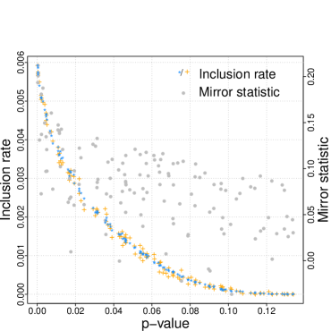
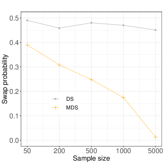
To illustrate Proposition 4, we fix p=800๐‘800p=800, and consider a weak separation between p1subscript๐‘1p_{1} and p2subscript๐‘2p_{2} by setting p1<p2subscript๐‘1subscript๐‘2p_{1}<p_{2} with p1=0.020subscript๐‘10.020p_{1}=0.020 and p2=0.021subscript๐‘20.021p_{2}=0.021. That is, we sample Xiโ€‹1subscript๐‘‹๐‘–1X_{i1}โ€™s conditioning on ๐‘ฟยฏ1=|ฮฆโ€‹(0.01)/n|subscriptยฏ๐‘ฟ1ฮฆ0.01๐‘›\bar{\bm{X}}_{1}=|\Phi(0.01)/\sqrt{n}| and Xiโ€‹2subscript๐‘‹๐‘–2X_{i2}โ€™s conditioning on ๐‘ฟยฏ2=๐‘ฟยฏ1โˆ’0.02/nsubscriptยฏ๐‘ฟ2subscriptยฏ๐‘ฟ10.02๐‘›\bar{\bm{X}}_{2}=\bar{\bm{X}}_{1}-0.02/\sqrt{n}. For jโ‰ฅ3๐‘—3j\geq 3, we set 20%percent2020\% of ฮผjsubscript๐œ‡๐‘—\mu_{j}โ€™s to be nonzero, and sample them independently from Nโ€‹(0,0.52)๐‘0superscript0.52N(0,0.5^{2}). We vary the sample size nโˆˆ{50,200,500,1000,5000}๐‘›5020050010005000n\in\{50,200,500,1000,5000\}, and estimate the swap probability โ„™โ€‹(M1<M2)โ„™subscript๐‘€1subscript๐‘€2\mathbbm{P}(M_{1}<M_{2}) for DS and โ„™โ€‹(I1<I2)โ„™subscript๐ผ1subscript๐ผ2\mathbbm{P}(I_{1}<I_{2}) for MDS over 500 independent runs. For DS, we construct the mirror statistics following (6). For MDS, we set the number of DS replications to be m=10โ€‹n๐‘š10๐‘›m=10n. The results in Figure 2 empirically validate Proposition 4. The left panel shows that for MDS, the swap probability โ„™โ€‹(I1<I2)โ„™subscript๐ผ1subscript๐ผ2\mathbbm{P}(I_{1}<I_{2}) gets very close to 0 when the sample size is large enough (say, nโ‰ฅ5000๐‘›5000n\geq 5000). However, for DS, the swap probability โ„™โ€‹(M1<M2)โ„™subscript๐‘€1subscript๐‘€2\mathbbm{P}(M_{1}<M_{2}) approximately remains as a constant (slightly below 0.5) as the sample size increases.
Refer to caption
Refer to caption
Figure 2: Comparison of DS and MDS on the Normal means model. Given the two p-values p1,p2subscript๐‘1subscript๐‘2p_{1},p_{2} with p1<p2subscript๐‘1subscript๐‘2p_{1}<p_{2}, the left panel plots the estimated swap probability, i.e., โ„™โ€‹(M1<M2)โ„™subscript๐‘€1subscript๐‘€2\mathbbm{P}(M_{1}<M_{2}) for DS and โ„™โ€‹(I1<I2)โ„™subscript๐ผ1subscript๐ผ2\mathbbm{P}(I_{1}<I_{2}) for MDS, against the sample size n๐‘›n. The right panel plots the inclusion rates of MDS and the mirror statistics of DS against the p-values. The detailed simulation setting can be found in Section 2.3.

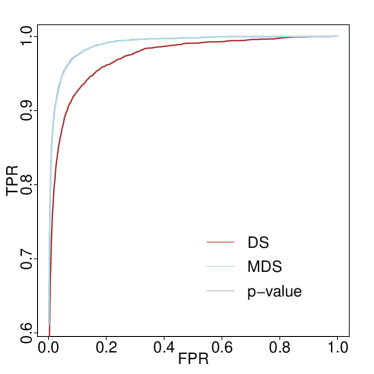
Proposition 4 also implies that for this simple model, when the sample size is reasonably large, the inclusion rates and the p-values nearly yield the same rankings of ฮผjsubscript๐œ‡๐‘—\mu_{j}โ€™s with high probability. To illustrate this, we consider a similar simulation setting as above with the sample size n=1000๐‘›1000n=1000, but without fixing ๐‘ฟยฏ1subscriptยฏ๐‘ฟ1\bar{\bm{X}}_{1} or ๐‘ฟยฏ2subscriptยฏ๐‘ฟ2\bar{\bm{X}}_{2}. In the right panel of Figure 2, we plot the inclusion rates (blue โ€œโˆ—โˆ—\astโ€ and orange โ€œ+โ€) of MDS and the mirror statistics of DS (grey โ€œโ‹…โ‹…\cdotโ€) against the p-values. For MDS, the blue โ€œโˆ—โˆ—\astโ€ and the orange โ€œ+โ€ refer to the estimated inclusion rates based upon m=10,000๐‘š10000m=10,000 and m=400๐‘š400m=400 DS replications, respectively. We see that the rankings of ฮผjsubscript๐œ‡๐‘—\mu_{j}โ€™s given by the inclusion rates are significantly less noisy compared to the rankings by the mirror statistics, and the inclusion rate is approximately a monotone decreasing function of the p-value. Thus, for this simple model, MDS almost recovers the power loss of DS due to sample splitting since the p-values, which are calculated using the full data, summarize all the information related to the testing task. Figures 12 and 13 in Supplementary Materials provide more empirical comparisons between DS, MDS and BHq across various signal strengths.

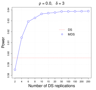
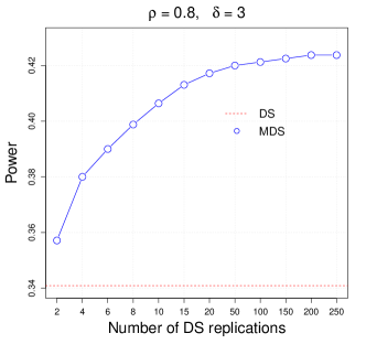
Ideally, we would like to conduct as many sample splits as possible for MDS so as to estimate the inclusion rates accurately. In practice, however, we find that the power of MDS no longer improves much after a relatively small number of DS replications (say, m=๐‘šabsentm= 100 or 200). See Figure 12 in Supplementary Materials and Figure 4 in Section 4.1 for some empirical evidences on the Normal means model and linear models, respectively. For the Normal means model, Figure 2 shows that increasing m๐‘šm from 400 to 10,000 leads to slightly less noisy rankings of ฮผjsubscript๐œ‡๐‘—\mu_{j}โ€™s by the inclusion rates.

3 Specializations for Different Statistical Models

In this section, we discuss how we construct the coefficients ๐œท^bold-^๐œท\bm{\widehat{\beta}} for linear and Gaussian graphical models. Our main concerns are that (1) the coefficients shall satisfy the symmetry assumption (Assumption 1); (2) the mirror statistics of the null features are weakly correlated (Assumption 2). Throughout this section, we split the data into two parts of equal size.

3.1 Linear models

Assuming that the true data generating process is ๐’š=๐‘ฟโ€‹๐œทโ‹†+ฯต๐’š๐‘ฟsuperscript๐œทโ‹†bold-italic-ฯต\bm{y}=\bm{X}\bm{\beta}^{\star}+\bm{\epsilon}, where ฯตโˆผNโ€‹(๐ŸŽ,ฯƒ2โ€‹In)similar-tobold-italic-ฯต๐‘0superscript๐œŽ2subscript๐ผ๐‘›\bm{\epsilon}\sim N(\bm{0},\sigma^{2}I_{n}), we consider the random-design scenario, in which each row of the design matrix ๐‘ฟ๐‘ฟ\bm{X} independently follows a p๐‘p-dimensional distribution with a covariance matrix ฮฃฮฃ\Sigma. In the context of feature selection, the true coefficient ๐œทโ‹†superscript๐œทโ‹†\bm{\beta}^{\star} is often assumed to be sparse, and the goal is to identify the set S1={j,ฮฒjโ‹†โ‰ 0}subscript๐‘†1๐‘—subscriptsuperscript๐›ฝโ‹†๐‘—0S_{1}=\{j,\ \beta^{\star}_{j}\neq 0\}.

We consider a Lasso + OLS procedure described as follows. On the first half of the data (๐’š(1),๐‘ฟ(1))superscript๐’š1superscript๐‘ฟ1(\bm{y}^{(1)},\bm{X}^{(1)}), we run Lasso for dimension reduction. Let ๐œท^(1)superscript^๐œท1\widehat{\bm{\beta}}^{(1)} be the estimated regression coefficients and denote S^(1)={j,ฮฒ^j(1)โ‰ 0}superscript^๐‘†1๐‘—subscriptsuperscript^๐›ฝ1๐‘—0\widehat{S}^{(1)}=\{j,\ \widehat{\beta}^{(1)}_{j}\neq 0\}. Being restricted to the subset of features S^(1)superscript^๐‘†1\widehat{S}^{(1)} selected by Lasso, we run OLS using the second half of the data (๐’š(2),๐‘ฟ(2))superscript๐’š2superscript๐‘ฟ2(\bm{y}^{(2)},\bm{X}^{(2)}) to obtain the estimated coefficients ๐œท^(2)superscript^๐œท2\widehat{\bm{\beta}}^{(2)}. We then construct the mirror statistics by (1) using ๐œท^(1)superscriptbold-^๐œท1\bm{\widehat{\beta}}^{(1)} and ๐œท^(2)superscriptbold-^๐œท2\bm{\widehat{\beta}}^{(2)}.

The symmetry assumption is satisfied if the sure screening property holds for Lasso, that is, all the relevant features are selected by Lasso in the first step. If this is the case, for any selected null feature jโˆˆS0โˆฉS^(1)๐‘—subscript๐‘†0superscript^๐‘†1j\in S_{0}\cap\widehat{S}^{(1)}, its second coefficient ฮฒ^j(2)superscriptsubscript^๐›ฝ๐‘—2\widehat{\beta}_{j}^{(2)} follows a centered Normal distribution conditioning on ๐‘ฟ(2)superscript๐‘ฟ2\bm{X}^{(2)}, thus is symmetric about 0. For Lasso, sufficient conditions for the sure screening property have been well established in the literature (e.g., see Remark 2). More generally, we can substitute Lasso by any other dimension reduction method as long as the sure screening property holds with probability approaching 1. For the weak dependence assumption, we calibrate the correlation structure among the mirror statistics using Mehlerโ€™s identity (Kotz etย al., 2000), and show that the weak dependence assumption holds with probability approaching 1 under the regularity condition and the tail condition in Assumption 3. Proposition 5 establishes the desired FDR control property for both DS and MDS.

Assumption 3

  1. 1.

    (Signal strength condition) minjโˆˆS1โก|ฮฒjโ‹†|โ‰ซp1โ€‹logโกp/nmuch-greater-thansubscript๐‘—subscript๐‘†1subscriptsuperscript๐›ฝโ‹†๐‘—subscript๐‘1๐‘๐‘›\min_{j\in S_{1}}|\beta^{\star}_{j}|\gg\sqrt{p_{1}\log p/n}.

  2. 2.

    (Regularity condition) 1/c<ฮปminโ€‹(ฮฃ)โ‰คฮปmaxโ€‹(ฮฃ)<c1๐‘subscript๐œ†ฮฃsubscript๐œ†ฮฃ๐‘1/c<\lambda_{\min}(\Sigma)\leq\lambda_{\max}(\Sigma)<c for some c>0๐‘0c>0.

  3. 3.

    (Tail condition) ๐‘ฟโ€‹ฮฃโˆ’1/2๐‘ฟsuperscriptฮฃ12\bm{X}\Sigma^{-1/2} has independent sub-Gaussian rows.

  4. 4.

    (Sparsity condition) p1=oโ€‹(n/logโกp)subscript๐‘1๐‘œ๐‘›๐‘p_{1}=o(n/\log p).

Proposition 5

Consider both DS and MDS, of which the two regression coefficients ๐›ƒ^(1)superscript^๐›ƒ1\widehat{\bm{\beta}}^{(1)} and ๐›ƒ^(2)superscript^๐›ƒ2\widehat{\bm{\beta}}^{(2)} are constructed using the Lasso + OLS procedure. For any designated FDR control level qโˆˆ(0,1)๐‘ž01q\in(0,1), under Assumption 3, we have

lim supn,pโ†’โˆžFDRโ‰คqandlim infn,pโ†’โˆžPower=1formulae-sequencesubscriptlimit-supremumโ†’๐‘›๐‘FDR๐‘žandsubscriptlimit-infimumโ†’๐‘›๐‘Power1\limsup_{n,p\to\infty}\text{FDR}\leq q\ \ \ \text{and}\ \ \ \liminf_{n,p\to\infty}\text{Power}=1

in the asymptotic regime where logโกp=oโ€‹(nฮพ)๐‘๐‘œsuperscript๐‘›๐œ‰\log p=o(n^{\xi}) for some ฮพโˆˆ(0,1)๐œ‰01\xi\in(0,1).

Remark 2

The sure screening property is implied by the signal strength condition and the compatibility condition (Vanย de Geer and Bรผhlmann, 2009). The compatibility condition means that the sample covariance matrix ฮฃ^^ฮฃ\widehat{\Sigma} of features satisfies ฯ•โ€‹(ฮฃ^,S1)โ‰ฅฯ•0italic-ฯ•^ฮฃsubscript๐‘†1subscriptitalic-ฯ•0\phi(\widehat{\Sigma},S_{1})\geq\phi_{0} for some ฯ•0>0subscriptitalic-ฯ•00\phi_{0}>0, in which ฯ•โ€‹(ฮฃ^,S)italic-ฯ•^ฮฃ๐‘†\phi(\widehat{\Sigma},S) is defined for any subset SโŠ†{1,โ€ฆ,p}๐‘†1โ€ฆ๐‘S\subseteq\{1,\ldots,p\} as

ฯ•2โ€‹(ฮฃ^,S)=min๐œฝโˆˆโ„pโก{|S|โ€‹๐œฝโŠบโ€‹ฮฃ^โ€‹๐œฝโ€–๐œฝSโ€–12:๐œฝโˆˆโ„p,โ€–๐œฝScโ€–1โ‰ค3โ€‹โ€–๐œฝSโ€–1}.superscriptitalic-ฯ•2^ฮฃ๐‘†subscript๐œฝsuperscriptโ„๐‘:๐‘†superscript๐œฝโŠบ^ฮฃ๐œฝsuperscriptsubscriptnormsubscript๐œฝ๐‘†12formulae-sequence๐œฝsuperscriptโ„๐‘subscriptnormsubscript๐œฝsuperscript๐‘†๐‘13subscriptnormsubscript๐œฝ๐‘†1\phi^{2}(\widehat{\Sigma},S)=\min_{\bm{\theta}\in\mathbbm{R}^{p}}\left\{\frac{|S|\bm{\theta}^{\intercal}\widehat{\Sigma}\bm{\theta}}{||\bm{\theta}_{S}||_{1}^{2}}:\ \bm{\theta}\in\mathbbm{R}^{p},\ ||\bm{\theta}_{S^{c}}||_{1}\leq 3||\bm{\theta}_{S}||_{1}\right\}.

By Theorem 2.4 in Javanmard and Montanari (2014), if the regularity condition and the tail condition in Assumption 3 hold, the compatibility condition holds with high probability for nโ‰ฅcโ€‹p1โ€‹logโก(p/p1)๐‘›๐‘subscript๐‘1๐‘subscript๐‘1n\geq cp_{1}\log(p/p_{1}). Furthermore, assuming that the compatibility condition holds, with a properly chosen regularization parameter, the Lasso regression coefficients ๐›ƒ^^๐›ƒ\widehat{\bm{\beta}} satisfy

โ€–๐œท^โˆ’๐œทโ‹†โ€–2=opโ€‹(p1โ€‹logโกp/n).subscriptnorm^๐œทsuperscript๐œทโ‹†2subscript๐‘œ๐‘subscript๐‘1๐‘๐‘›||\widehat{\bm{\beta}}-{\bm{\beta}}^{\star}||_{2}=o_{p}(\sqrt{p_{1}\log p/n}).

Together with the signal strength condition, we see that the sure screening property holds with probability approaching 1. The sure screening property also appears crucial in many other related methods, e.g., see Barber and Candรจs (2019) and Fan etย al. (2020) for the knockoff filter.

Besides Proposition 5, more detailed power analyses of DS and MDS are still unknown and await future investigations. In comparison, some theoretical studies on the power of knockoff filters begin to appear recently. For example, Fan etย al. (2020) showed that, under a similar signal strength condition, i.e., minjโˆˆS1โก|ฮฒjโ‹†|โ‰ซlogโกp/nmuch-greater-thansubscript๐‘—subscript๐‘†1superscriptsubscript๐›ฝ๐‘—โ‹†๐‘๐‘›\min_{j\in S_{1}}|\beta_{j}^{\star}|\gg\sqrt{\log p/n}, and when features follow a multivariate Normal distribution with known covariance matrix, the model-X knockoff filter has asymptotic power one. Moving beyond this ideal scenario, i.e, when the covariance matrix of features is unknown, they proposed a modified knockoff procedure based on data splitting and show that the power of the modified procedure converges to one asymptotically if the sure screening property holds. In a different asymptotic regime where both n/p๐‘›๐‘n/p and p1/psubscript๐‘1๐‘p_{1}/p converge to some fixed constants, the power analysis has also been rigorously carried out in the setting with i.i.d. Gaussian features (e.g., see Weinstein etย al. (2017) for the โ€œcountingโ€-knockoffs, and see Weinstein etย al. (2020) and Wang and Janson (2020) for the model-X knockoff filter and also the conditional randomization test). For correlated designs, Liu and Rigollet (2019) provided some explicit conditions under which the knockoff filter enjoys FDR zero and power one asymptotically. Under the weak-and-rare signal setting, Ke etย al. (2020) analyzed both the knockoff filter and the Gaussian mirror method for some special covariance structures, identifying key components that can influence the power of these methods.

Compared to BHq, one main advantage of DS and MDS is that they do not require p-values, which are generally difficult to obtain in high-dimensional linear models. Notable theoretical contributions on constructing valid p-values include the post-selection inference and the debiased Lasso procedure. Conditioning on the selected model, the post-selection inference derives the exact distribution of the regression coefficients. Details have been worked out for several popular selection procedures including Lasso (Lee etย al., 2016), the forward stepwise regression, and the least angle regression (Tibshirani etย al., 2016). However, this type of theory is mostly developed case by case, and cannot be easily generalized to other selection procedures. The debiased Lasso procedure removes the biases in the Lasso regression coefficients so that they enjoy the asymptotic Normality under certain conditions (Van de Geer etย al., 2014; Zhang and Zhang, 2014; Javanmard and Montanari, 2014). We refer the readers to Javanmard and Javadi (2019) for an FDR control procedure that applies BHq to the p-values obtained via the debiased Lasso procedure.

BHq may still perform poorly using the p-values obtained from the aforementioned methods. For the post-selection inference, the transformation that converts the regression coefficients to p-values may seriously dilute the true signals. For the debiased-Lasso procedure, the asymptotic null p-values may appear highly non-uniform in finite-sample cases (e.g., see some empirical evidences in Dezeure etย al. (2015) and Candรจs etย al. (2018)). To avoid using p-values, several authors suggested selecting a proper penalty in penalized regressions based upon the p-value cutoff in order to achieve FDR control. We refer the readers to Benjamini and Gavrilov (2009) and Bogdan etย al. (2015) for more details.

We conclude this section on linear models by briefly commenting on how to use the proposed methods in the low-dimensional setting with n/pโ†’โˆžโ†’๐‘›๐‘n/p\to\infty. For the first half of the data (๐’š(1),๐‘ฟ(1))superscript๐’š1superscript๐‘ฟ1(\bm{y}^{(1)},\bm{X}^{(1)}), on a case-by-case basis, we can choose any sensible method (e.g., OLS, Lasso, ridge, or other regularization methods) to obtain the coefficients ๐œท^(1)superscriptbold-^๐œท1\bm{\widehat{\beta}}^{(1)}. For (๐’š(2),๐‘ฟ(2))superscript๐’š2superscript๐‘ฟ2(\bm{y}^{(2)},\bm{X}^{(2)}), we run OLS using all features to obtain the coefficients ๐œท^(2)superscriptbold-^๐œท2\bm{\widehat{\beta}}^{(2)}. The symmetry assumption is automatically satisfied since the model in the OLS step is well specified. The weak dependence assumption still holds under the regularity condition and the tail condition in Assumption 3. Therefore, similar to Proposition 5, we can show that DS asymptotically controls the FDR without requiring the signal strength and the sparsity conditions. We note that in the low-dimensional setting, the Lasso + OLS procedure is also applicable as long as Assumption 3 is satisfied, and can be still favorable if both n๐‘›n, p๐‘p are large and the relevant features are sparse. In particular, in the asymptotic regime where p/nโ†’cโˆˆ(0,1/2)โ†’๐‘๐‘›๐‘012p/n\to c\in(0,1/2), it can be problematic to directly run OLS on (๐’š(2),๐‘ฟ(2))superscript๐’š2superscript๐‘ฟ2(\bm{y}^{(2)},\bm{X}^{(2)}) with all features since the resulting covariance matrix of ๐œท^(2)superscriptbold-^๐œท2\bm{\widehat{\beta}}^{(2)} may be ill-conditioned, thus the weak dependence assumption may not hold.

3.2 Gaussian graphical models

Suppose ๐‘ฟ=(X1,โ€ฆ,Xp)๐‘ฟsubscript๐‘‹1โ€ฆsubscript๐‘‹๐‘\bm{X}=(X_{1},\ldots,X_{p}) follows a p๐‘p-dimensional multivariate Normal distribution Nโ€‹(๐,ฮฃ)๐‘๐ฮฃN(\bm{\mu},\Sigma). Let ฮ›=ฮฃโˆ’1=(ฮปiโ€‹j)ฮ›superscriptฮฃ1subscript๐œ†๐‘–๐‘—\Lambda=\Sigma^{-1}=(\lambda_{ij}) be the precision matrix. Without loss of generality, we assume ๐=๐ŸŽ๐0\bm{\mu}=\bm{0}. One can define a corresponding Gaussian graphical model (V,E)๐‘‰๐ธ(V,E), in which the set of vertices is V=(X1,โ€ฆ,Xp)๐‘‰subscript๐‘‹1โ€ฆsubscript๐‘‹๐‘V=(X_{1},\ldots,X_{p}), and there is an edge between two different vertices Xisubscript๐‘‹๐‘–X_{i} and Xjsubscript๐‘‹๐‘—X_{j} if Xisubscript๐‘‹๐‘–X_{i} and Xjsubscript๐‘‹๐‘—X_{j} are conditionally dependent given {Xk,kโ‰ i,j}formulae-sequencesubscript๐‘‹๐‘˜๐‘˜๐‘–๐‘—\{X_{k},\ k\neq i,j\}. The graph estimation can be recast as a nodewise regression problem. To see this, for each vertex Xjsubscript๐‘‹๐‘—X_{j}, we can write

Xj=๐‘ฟโˆ’jโŠบโ€‹๐œทj+ฯตjwith๐œทj=โˆ’ฮปjโ€‹jโˆ’1โ€‹ฮ›โˆ’j,j,formulae-sequencesubscript๐‘‹๐‘—superscriptsubscript๐‘ฟ๐‘—โŠบsuperscript๐œท๐‘—subscriptitalic-ฯต๐‘—withsuperscript๐œท๐‘—superscriptsubscript๐œ†๐‘—๐‘—1subscriptฮ›๐‘—๐‘—X_{j}=\bm{X}_{-j}^{\intercal}\bm{\beta}^{j}+\epsilon_{j}\ \ \ \text{with}\ \ \bm{\beta}^{j}=-\lambda_{jj}^{-1}\Lambda_{-j,j},

where ฯตjsubscriptitalic-ฯต๐‘—\epsilon_{j}, independent of ๐‘ฟโˆ’jsubscript๐‘ฟ๐‘—\bm{X}_{-j}, follows a centered Normal distribution. Thus, ฮปiโ€‹j=0subscript๐œ†๐‘–๐‘—0\lambda_{ij}=0 implies that Xisubscript๐‘‹๐‘–X_{i} and Xjsubscript๐‘‹๐‘—X_{j} are conditionally independent. We denote the neighborhood of vertex Xjsubscript๐‘‹๐‘—X_{j} as nโ€‹ej={k:kโ‰ j,ฮฒkjโ‰ 0}๐‘›subscript๐‘’๐‘—conditional-set๐‘˜formulae-sequence๐‘˜๐‘—subscriptsuperscript๐›ฝ๐‘—๐‘˜0ne_{j}=\{k:\ k\neq j,\ \beta^{j}_{k}\neq 0\}. Given i.i.d. samples ๐‘ฟ1,โ€ฆ,๐‘ฟnsubscript๐‘ฟ1โ€ฆsubscript๐‘ฟ๐‘›\bm{X}_{1},\ldots,\bm{X}_{n} from Nโ€‹(๐,ฮฃ)๐‘๐ฮฃN(\bm{\mu},\Sigma), it is natural to consider first recovering the support of each ๐œทjsuperscript๐œท๐‘—\bm{\beta}^{j} using a feature selection method such as Lasso (Meinshausen and Bรผhlmann, 2006), and then combining all the nodewise selection results properly to estimate the graph. In view of this, for a designated level qโˆˆ(0,1)๐‘ž01q\in(0,1), we propose an FDR control procedure as summarized in Algorithm 3.

Algorithm 3 False discovery rate control in Gaussian graphical models via a single data split.
  1. 1.

    Targeting at the level q/2๐‘ž2q/2, apply the Lasso + OLS procedure (see Section 3.1) to each nodewise regression. Denote the nodewise selection results as nโ€‹e^j={k:kโ‰ j,ฮฒ^kjโ‰ 0}subscript^๐‘›๐‘’๐‘—conditional-set๐‘˜formulae-sequence๐‘˜๐‘—subscriptsuperscript^๐›ฝ๐‘—๐‘˜0\widehat{ne}_{j}=\{k:\ k\neq j,\ \widehat{\beta}^{j}_{k}\neq 0\} for jโˆˆ{1,โ€ฆ,p}๐‘—1โ€ฆ๐‘j\in\{1,\ldots,p\}.

  2. 2.

    Combine the nodewise selection results using the OR rule to estimate the graph:

    E^ORsubscript^๐ธOR\displaystyle\widehat{E}_{\text{OR}} ={(i,j):iโˆˆnโ€‹e^jโ€‹orโ€‹jโˆˆnโ€‹e^i}.absentconditional-set๐‘–๐‘—๐‘–subscript^๐‘›๐‘’๐‘—or๐‘—subscript^๐‘›๐‘’๐‘–\displaystyle=\{(i,j):\ i\in\widehat{ne}_{j}\ \text{or}\ j\in\widehat{ne}_{i}\}.

A heuristic justification of the proposed method is given below:

FDP =#โ€‹{(i,j)โˆˆE^OR,(i,j)โˆ‰E}|E^OR|โˆจ1โ‰คโˆ‘j=1p#โ€‹{iโˆ‰nโ€‹ej,iโˆˆnโ€‹e^j}12โ€‹โˆ‘j=1p#โ€‹{iโˆˆnโ€‹e^j}โˆจ1=โˆ‘j=1p#โ€‹{iโˆ‰nโ€‹ej,Mjโ€‹i>ฯ„q/2j}12โ€‹โˆ‘j=1p#โ€‹{Mjโ€‹i>ฯ„q/2j}โˆจ1absent#formulae-sequence๐‘–๐‘—subscript^๐ธOR๐‘–๐‘—๐ธsubscript^๐ธOR1superscriptsubscript๐‘—1๐‘#formulae-sequence๐‘–๐‘›subscript๐‘’๐‘—๐‘–subscript^๐‘›๐‘’๐‘—12superscriptsubscript๐‘—1๐‘#๐‘–subscript^๐‘›๐‘’๐‘—1superscriptsubscript๐‘—1๐‘#formulae-sequence๐‘–๐‘›subscript๐‘’๐‘—subscript๐‘€๐‘—๐‘–superscriptsubscript๐œ๐‘ž2๐‘—12superscriptsubscript๐‘—1๐‘#subscript๐‘€๐‘—๐‘–superscriptsubscript๐œ๐‘ž2๐‘—1\displaystyle=\frac{\#\{(i,j)\in\widehat{E}_{\text{OR}},(i,j)\notin E\}}{|\widehat{E}_{\text{OR}}|\vee 1}\leq\frac{\sum_{j=1}^{p}\#\{i\notin ne_{j},i\in\widehat{ne}_{j}\}}{\frac{1}{2}\sum_{j=1}^{p}\#\{i\in\widehat{ne}_{j}\}\vee 1}=\frac{\sum_{j=1}^{p}\#\{i\notin ne_{j},M_{ji}>\tau_{q/2}^{j}\}}{\frac{1}{2}\sum_{j=1}^{p}\#\{M_{ji}>\tau_{q/2}^{j}\}\vee 1} (7)
โ‰ˆโˆ‘j=1p#โ€‹{iโˆ‰nโ€‹ej,Mjโ€‹i<โˆ’ฯ„q/2j}12โ€‹โˆ‘j=1p#โ€‹{Mjโ€‹i>ฯ„q/2j}โˆจ1โ‰ค2โ€‹max1โ‰คjโ‰คpโก#โ€‹{iโˆ‰nโ€‹ej,Mjโ€‹i<โˆ’ฯ„q/2j}#โ€‹{Mjโ€‹i>ฯ„q/2j}โˆจ1โ‰คq.absentsuperscriptsubscript๐‘—1๐‘#formulae-sequence๐‘–๐‘›subscript๐‘’๐‘—subscript๐‘€๐‘—๐‘–superscriptsubscript๐œ๐‘ž2๐‘—12superscriptsubscript๐‘—1๐‘#subscript๐‘€๐‘—๐‘–superscriptsubscript๐œ๐‘ž2๐‘—12subscript1๐‘—๐‘#formulae-sequence๐‘–๐‘›subscript๐‘’๐‘—subscript๐‘€๐‘—๐‘–superscriptsubscript๐œ๐‘ž2๐‘—#subscript๐‘€๐‘—๐‘–superscriptsubscript๐œ๐‘ž2๐‘—1๐‘ž\displaystyle\approx\frac{\sum_{j=1}^{p}\#\{i\notin ne_{j},M_{ji}<-\tau_{q/2}^{j}\}}{\frac{1}{2}\sum_{j=1}^{p}\#\{M_{ji}>\tau_{q/2}^{j}\}\vee 1}\leq 2\max_{1\leq j\leq p}\frac{\#\{i\notin ne_{j},M_{ji}<-\tau_{q/2}^{j}\}}{\#\{M_{ji}>\tau_{q/2}^{j}\}\vee 1}\leq q.

For the j๐‘—j-th nodewise regression, Mjโ€‹isubscript๐‘€๐‘—๐‘–M_{ji} is the mirror statistic of Xisubscript๐‘‹๐‘–X_{i}, iโ‰ j๐‘–๐‘—i\neq j, and ฯ„q/2jsuperscriptsubscript๐œ๐‘ž2๐‘—\tau_{q/2}^{j} is the selection cutoff of the mirror statistics. The first inequality in Equation (7) is based on the fact that each edge can be selected at most twice. The approximation in the middle utilizes the symmetric property of the mirror statistics. The second to last inequality follows from the elementary inequality that (โˆ‘nan)/(โˆ‘nbn)โ‰คmaxnโกan/bnsubscript๐‘›subscript๐‘Ž๐‘›subscript๐‘›subscript๐‘๐‘›subscript๐‘›subscript๐‘Ž๐‘›subscript๐‘๐‘›\left(\sum_{n}a_{n}\right)/\left(\sum_{n}b_{n}\right)\leq\max_{n}a_{n}/b_{n} for anโ‰ฅ0,bn>0formulae-sequencesubscript๐‘Ž๐‘›0subscript๐‘๐‘›0a_{n}\geq 0,\ b_{n}>0.

We note that there are potentially two strategies to implement MDS for Gaussian graphical models: (i) We can apply MDS in each nodewise regression (Step 1 in Algorithm 3) and then aggregate all the selection results using the OR rule; (ii) We can replicate the whole procedure in Algorithm 3 (both Steps 1 and 2) multiple times, and use MDS to aggregate all the selections results by Algorithm 2. Empirically we found that both strategies achieve FDR control, and the first one tends to have a higher power. Throughout the following theoretical justification and simulation studies, we focus on the first strategy for MDS.

Let s=maxjโˆˆ{1,โ€ฆ,p}โก|nโ€‹ej|๐‘ subscript๐‘—1โ€ฆ๐‘๐‘›subscript๐‘’๐‘—s=\max_{j\in\{1,\ldots,p\}}|ne_{j}|. To theoretically justify our methods, we first show that with probability approaching 1, the symmetry assumption is simultaneously satisfied in all nodewise regressions under the following assumptions.

Assumption 4

  1. 1.

    (Regularity condition) cโ‰คฮปminโ€‹(ฮฃ)โ‰คฮปmaxโ€‹(ฮฃ)โ‰ค1/c๐‘subscript๐œ†ฮฃsubscript๐œ†ฮฃ1๐‘c\leq\lambda_{\min}(\Sigma)\leq\lambda_{\max}(\Sigma)\leq 1/c for some c>0๐‘0c>0.

  2. 2.

    (Sparsity condition) s=oโ€‹(n/logโกp)๐‘ ๐‘œ๐‘›๐‘s=o(n/\log p).

  3. 3.

    (Signal strength condition) minโก{|ฮปiโ€‹j|:ฮปiโ€‹jโ‰ 0}โ‰ซsโ€‹logโกp/nmuch-greater-than:subscript๐œ†๐‘–๐‘—subscript๐œ†๐‘–๐‘—0๐‘ ๐‘๐‘›\min\{|\lambda_{ij}|:\lambda_{ij}\neq 0\}\gg\sqrt{s\log p/n}.

Assumption 4 serves the same purpose as Assumption 3 for linear models (e.g., ensure that the sure screening property holds simultaneously in all nodewise regressions; see Remark 2). Similar assumptions also appear in Liu (2013) and Meinshausen and Bรผhlmann (2006). Under Assumption 4, we have the following proposition.

Proposition 6

Under Assumption 4, as n,pโ†’โˆžโ†’๐‘›๐‘n,p\to\infty satisfying logโกp=oโ€‹(n)๐‘๐‘œ๐‘›\log p=o(n), the symmetry assumption (Assumption 1) is simultaneously satisfied in all nodewise regressions with probability approaching 1.

Similar to linear models, the weak dependence assumption is implied by the regularity condition in Assumption 4. The following proposition shows that both DS and MDS asymptotically control the FDR.

Proposition 7

Assume that Assumption 4 holds and that minjโˆˆ{1,โ€ฆ,p}โก|nโ€‹ej|/logโกpโ†’โˆžโ†’subscript๐‘—1โ€ฆ๐‘๐‘›subscript๐‘’๐‘—๐‘\min_{j\in\{1,\ldots,p\}}|ne_{j}|/\log p\to\infty. For any designated FDR control level qโˆˆ(0,1)๐‘ž01q\in(0,1), both DS (see Algorithm 3) and the corresponding MDS procedure achieve

lim supn,pโ†’โˆžFDRโ‰คqandlim infn,pโ†’โˆžPower=1formulae-sequencesubscriptlimit-supremumโ†’๐‘›๐‘FDR๐‘žandsubscriptlimit-infimumโ†’๐‘›๐‘Power1\limsup_{n,p\to\infty}\text{FDR}\leq q\ \ \ \text{and}\ \ \ \liminf_{n,p\to\infty}\text{Power}=1

in the asymptotic regime where logโกp=oโ€‹(nฮพ)๐‘๐‘œsuperscript๐‘›๐œ‰\log p=o(n^{\xi}) for some ฮพโˆˆ(0,1)๐œ‰01\xi\in(0,1).

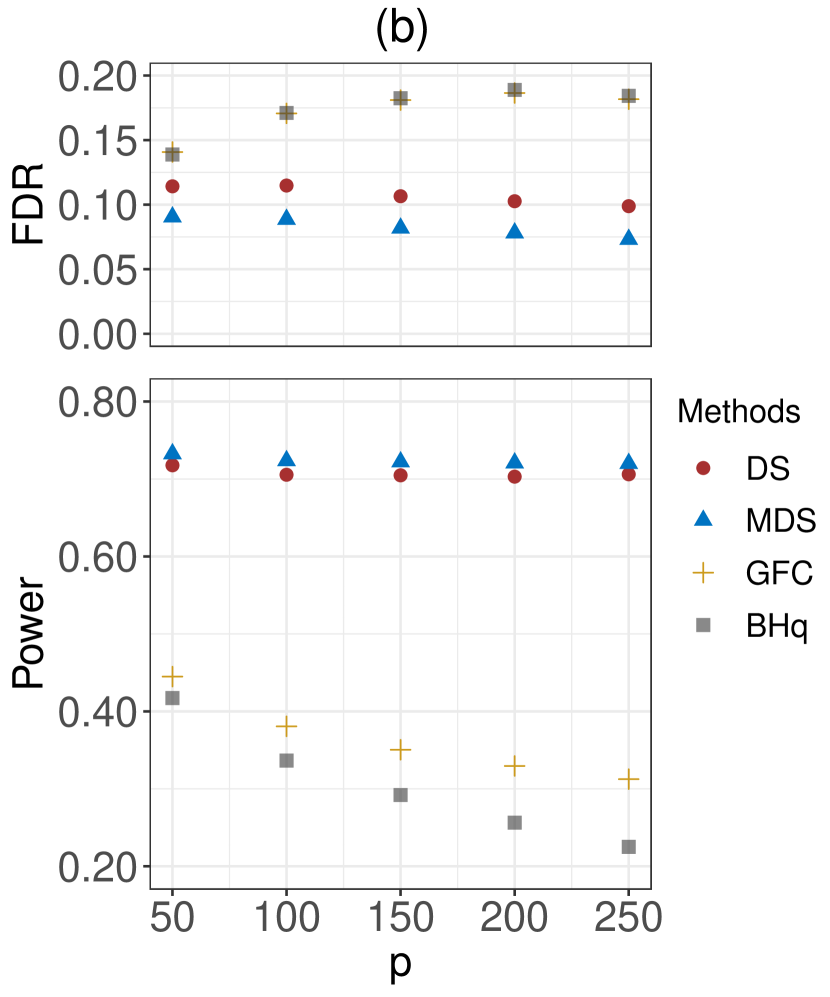
The assumption minjโˆˆ{1,โ€ฆ,p}โก|nโ€‹ej|/logโกpโ†’โˆžโ†’subscript๐‘—1โ€ฆ๐‘๐‘›subscript๐‘’๐‘—๐‘\min_{j\in\{1,\ldots,p\}}|ne_{j}|/\log p\to\infty is mainly for the technical purpose so that a union bound can be applied for all nodewise regressions. Empirically, we find that the data-splitting methods and the GFC method proposed in Liu (2013) are effective in quite different scenarios. GFC tends to work well if the underlying true graph is ultra-sparse, i.e., the nodewise sparsity is in the order of oโ€‹(n/(logโกp)3/2)๐‘œ๐‘›superscript๐‘32o(\sqrt{n}/(\log p)^{3/2}). In contrast, DS and MDS are capable of handling cases where the graph is not too sparse, but may suffer from the ultra-sparsity. A similar issue also exists in general knockoff-based methods, and we refer the readers to Li and Maathuis (2019) for relevant discussions.

4 Numerical Illustrations

4.1 Linear model

We simulate the response vector ๐’š๐’š\bm{y} from the linear model ๐’šnร—1=๐‘ฟnร—pโ€‹๐œทpร—1โ‹†+ฯตnร—1subscript๐’š๐‘›1subscript๐‘ฟ๐‘›๐‘subscriptsuperscript๐œทโ‹†๐‘1subscriptbold-italic-ฯต๐‘›1\bm{y}_{n\times 1}=\bm{X}_{n\times p}\bm{\beta}^{\star}_{p\times 1}+\bm{\epsilon}_{n\times 1} with ฯตโˆผNโ€‹(๐ŸŽ,In)similar-tobold-italic-ฯต๐‘0subscript๐ผ๐‘›\bm{\epsilon}\sim N(\bm{0},I_{n}), and randomly locate the signal index set S1subscript๐‘†1S_{1}. For jโˆˆS1๐‘—subscript๐‘†1j\in S_{1}, we sample ฮฒjโ‹†subscriptsuperscript๐›ฝโ‹†๐‘—\beta^{\star}_{j} from Nโ€‹(0,ฮดโ€‹logโกp/n)๐‘0๐›ฟ๐‘๐‘›N(0,\delta\sqrt{\log p/n}), and refer to ฮด๐›ฟ\delta as the signal strength. Throughout, the designated FDR control level is set to be q=0.1๐‘ž0.1q=0.1. The penalization parameter of Lasso is selected based on 10-fold cross-validation.

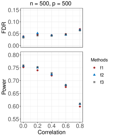
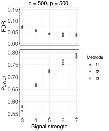
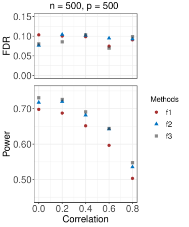
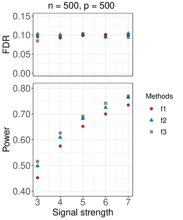
We first investigate the performance of DS/MDS using different mirror statistics constructed with f1,f2,f3subscript๐‘“1subscript๐‘“2subscript๐‘“3f_{1},f_{2},f_{3} specified in (2). We set the sample size n=500๐‘›500n=500, the number of features p=500๐‘500p=500, and the number of relevant features p1=50subscript๐‘150p_{1}=50. Each row of the design matrix is independently drawn from Nโ€‹(0,ฮฃ)๐‘0ฮฃN(0,\Sigma). We consider a similar setup as in Ma etย al. (2020), where ฮฃฮฃ\Sigma is a blockwise diagonal matrix of 10 Toeplitz submatrices whose off-diagonal entries linearly descend from ฯ๐œŒ\rho to 0. The detailed formula of ฮฃฮฃ\Sigma is given in (24) in Supplementary Materials, and we refer to it as the Toeplitz covariance matrix throughout. We vary the correlation ฯ๐œŒ\rho and the signal strength ฮด๐›ฟ\delta, and the results are summarized in Figure 3. We see that across different settings, all three choices of mirror statistics achieve FDR control, and f3subscript๐‘“3f_{3} yields the highest power. Proposition 1 shows that f3subscript๐‘“3f_{3} is optimal for orthogonal designs, and the empirical results suggest that f3subscript๐‘“3f_{3} might also be a good choice in more realistic settings. Among all the simulation studies described below, we construct the mirror statistics with f3subscript๐‘“3f_{3}. It is worth noting that the performance of MDS appears to be more robust to the choice of mirror statistics compared to DS (see Figure 14 in Supplementary Materials).
Refer to caption
Refer to caption
Figure 3: Empirical FDRs and powers of DS using three different mirror statistics constructed with f1,f2,f3subscript๐‘“1subscript๐‘“2subscript๐‘“3f_{1},f_{2},f_{3} specified in (2). Features are independently drawn from Nโ€‹(0,ฮฃ)๐‘0ฮฃN(0,\Sigma) with ฮฃฮฃ\Sigma being a Toeplitz covariance matrix. In the left panel, we fix the signal strength at ฮด=5๐›ฟ5\delta=5 and vary the correlation ฯ๐œŒ\rho. In the right panel, we fix the correlation at ฯ=0.4๐œŒ0.4\rho=0.4 and vary the signal strength ฮด๐›ฟ\delta. The number of relevant features is p1=50subscript๐‘150p_{1}=50 across all settings, and the designated FDR control level is q=0.1๐‘ž0.1q=0.1. Each dot in the figure represents the average from 50 independent runs.

We then examine the effect of the number of DS replications m๐‘šm on the power of MDS. With n=500๐‘›500n=500, p=500๐‘500p=500 and p1=50subscript๐‘150p_{1}=50, we generate features independently from Nโ€‹(0,ฮฃ)๐‘0ฮฃN(0,\Sigma) with ฮฃฮฃ\Sigma being a Toeplitz covariance matrix. We set the signal strength ฮด=3๐›ฟ3\delta=3 and test out two scenarios with the correlation ฯ=0.0๐œŒ0.0\rho=0.0 and ฯ=0.8๐œŒ0.8\rho=0.8. Figure 4 shows that the power of MDS monotonically increases with the number of DS replications m๐‘šm, and becomes relatively stable after mโ‰ฅ50๐‘š50m\geq 50. Empirical evidence suggests that it only requires a small number of DS replications to realize the full power of MDS. Thus, MDS is computationally more feasible for large data sets compared to other methods such as the knockoff filter and the Gaussian mirror method. In the following examples, we set m=50๐‘š50m=50 for MDS.

Refer to caption
Refer to caption
Figure 4: Empirical powers of MDS with different number of DS replications. Each row of the design matrix is independently drawn from Nโ€‹(0,ฮฃ)๐‘0ฮฃN(0,\Sigma) with ฮฃฮฃ\Sigma being a Toeplitz covariance matrix. The sample size is n=500๐‘›500n=500, the number of features is p=500๐‘500p=500, and the number of relevant features is p1=50subscript๐‘150p_{1}=50 in both settings. Over 50 independent runs, the blue dots and the red lines represent the average powers of MDS and DS, respectively.

We proceed to compare DS/MDS with two popular methods in high-dimensional settings under various design matrices: MBHq (Meinshausen etย al., 2009) and the model-X knockoff filter (Candรจs etย al., 2018). For their comparisons in low-dimenisonal settings, we refer the readers to Figures 15 and 16 in Supplementary Materials. For MBHq, we obtain 50 p-values for each feature via repeated sample splitting. More precisely, we run Lasso for feature screening on one half of the data, and calculate the p-values for the selected features by running OLS on the other half of the data. We then combine the p-values across different sample splits using the R package hdi.777https://cran.r-project.org/web/packages/hdi/hdi.pdf For the knockoff filter, we use the equi-correlated knockoffs, in which the covariance matrix of features is estimated using the R package knockoff.888https://cran.r-project.org/web/packages/knockoff/index.html For all the simulation settings in Section 4.1, we empirically found that the equi-correlated knockoffs yields a more powerful knockoff filter compared to the default asdp construction.

  1. 1.

    Normal design matrices. With n=800๐‘›800n=800, pโˆˆ{1000,2000}๐‘10002000p\in\{1000,2000\} and p1=50subscript๐‘150p_{1}=50, we generate features independently from Nโ€‹(0,ฮฃ)๐‘0ฮฃN(0,\Sigma) with ฮฃฮฃ\Sigma being a Toeplitz covariance matrix. We compare the performances of the competing methods under different correlations ฯ๐œŒ\rho and signal strengths ฮด๐›ฟ\delta. The results for p=2000๐‘2000p=2000 are summarized in Figure 5, and the results for p=1000๐‘1000p=1000 are summarized in Figure 17 in Supplementary Materials. The FDRs of all the four methods are under control across different settings. In terms of power, the knockoff filter and MDS are the two leading methods. MDS appears more powerful when features are more correlated, or when the signal strength is relatively weak, whereas the knockoff filter enjoys a higher power in the opposite regimes. We observed that MDS is more robust to highly correlated design matrices compared to the knockoff filter. Figure 19 in Supplementary Materials report the performances of the competing methods in the case where ฮฃฮฃ\Sigma has constant pairwise correlation ฯ๐œŒ\rho. We see that the knockoff filter appears significantly less powerful than MDS when ฯโ‰ฅ0.4๐œŒ0.4\rho\geq 0.4. The simulation results also suggest that MDS yields better rankings of features compared to DS, thus enjoys simultaneously a lower FDR and a higher power.
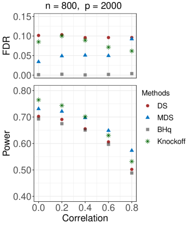
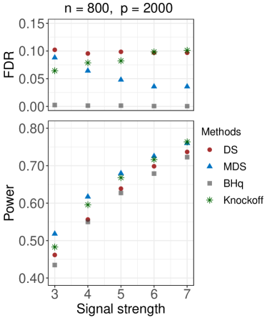
    Refer to caption
    Refer to caption
    Figure 5: Empirical FDRs and powers for linear models with Normal design matrices. Features are independently drawn from Nโ€‹(0,ฮฃ)๐‘0ฮฃN(0,\Sigma) with ฮฃฮฃ\Sigma being a Toeplitz covariance matrix. In the left panel, we fix the signal strength at ฮด=5๐›ฟ5\delta=5 and vary the correlation ฯ๐œŒ\rho. In the right panel, we fix the correlation at ฯ=0.5๐œŒ0.5\rho=0.5 and vary the signal strength ฮด๐›ฟ\delta. The designated FDR control level is q=0.1๐‘ž0.1q=0.1, and the number of relevant features is p1=50subscript๐‘150p_{1}=50 across all settings. Each dot in the figure represents the average from 50 independent runs.
  2. 2.

    Non-Normal design matrices. When the joint distribution of features is unknown and non-Normal, the performance of the knockoff filter is not guaranteed if the knockoffs are generated based upon a naive fit of the multivariate Normal distribution using the design matrix. We here illustrate the robustness of DS/MDS with respect to the non-Normality by considering the following two design matrices: (1) a two-component Gaussian mixture distribution centered at 0.5ร—๐Ÿ™p0.5subscript1๐‘0.5\times\mathbbm{1}_{p} and โˆ’0.5ร—๐Ÿ™p0.5subscript1๐‘-0.5\times\mathbbm{1}_{p}; (2) a centered multivariate t๐‘กt-distribution with 3 degrees of freedom. Throughout, the covariance matrix ฮฃฮฃ\Sigma is set to be a Toeplitz matrix. Note that in both scenarios, the marginal distribution of each feature is still unimodal, and does not differ much from the Normal distribution in appearance. We fix n=800๐‘›800n=800, p=2000๐‘2000p=2000, p1=70subscript๐‘170p_{1}=70, and test out different correlations ฯ๐œŒ\rho and signal strengths ฮด๐›ฟ\delta. The results are summarized in Figure 6. Because of the model misspecification in the knockoff construction, the knockoff filter appears over conservative when features follow a Gaussian mixture distribution, and loses FDR control when features follow a t๐‘กt-distribution. The latter is perhaps a more concerning issue in the context of controlled feature selection, although the performance of the knockoff filter can be potentially improved by carefully modeling the joint distribution of features based on some structural assumptions (e.g., see Sesia etย al. (2018)). In comparison, MDS maintains FDR control and enjoys a reasonably high power in both scenarios. We also note that, except being overly conservative, MBHq performs quite competitively in all settings.
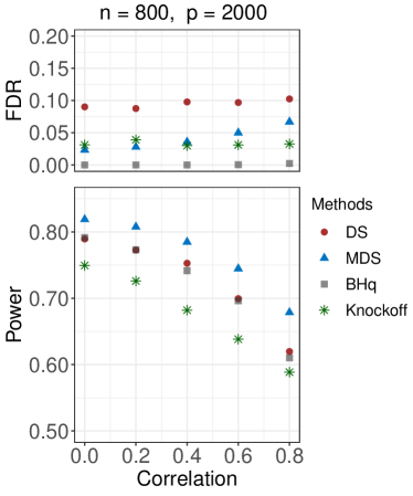
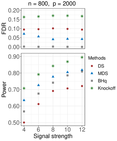
    Refer to caption
    Refer to caption
    Figure 6: Empirical FDRs and powers for linear models with non-Normal design matrices. In the left panel, features are independently drawn from a two-component mixture Normal distribution centered at 0.5ร—๐Ÿ™p0.5subscript1๐‘0.5\times\mathbbm{1}_{p} and โˆ’0.5ร—๐Ÿ™p0.5subscript1๐‘-0.5\times\mathbbm{1}_{p}. In the right panel, features are independently drawn from a centered multivariate t๐‘กt-distribution with 3 degrees of freedom. The covariance matrix ฮฃฮฃ\Sigma in both panels is set to be a Toeplitz matrix. In the left panel, we fix the signal strength at ฮด=8๐›ฟ8\delta=8 and vary the correlation ฯ๐œŒ\rho. In the right panel, we fix the correlation at ฯ=0.5๐œŒ0.5\rho=0.5 and vary the signal strength ฮด๐›ฟ\delta. The number of relevant features is p1=70subscript๐‘170p_{1}=70 across all settings, and the designated FDR control level is q=0.1๐‘ž0.1q=0.1. Each dot in the figure represents the average from 50 independent runs.
  3. 3.

    Real-data design matrices. We consider using the scRNAseq data in Hoffman etย al. (2020) as the design matrix. A total of 400 T47D A1โ€“2 human breast cancer cells were treated with 100 nM synthetic glucocorticoid dexamethasone (Dex). An scRNASeq experiment was performed after 18h of the Dex treatment, leading to a total of 400 samples of gene expressions for the treatment group. For the control group, there are 400 vehicle-treated control cells. An scRNAseq experiment was performed at the 18h timepoint to obtain the corresponding profile of gene expressions. After proper normalization, the final scRNAseq data999The data is available at https://www.ncbi.nlm.nih.gov/geo/query/acc.cgi?acc=GSE141834. contains 800 samples, each with 32,049 gene expressions. To further reduce the dimensionality, we first screen out the genes detected in fewer than 10% of cells, and then pick up the top p๐‘p most variable genes following Hoffman etย al. (2020). We fix p1=70subscript๐‘170p_{1}=70, and simulate the response vector ๐’š๐’š\bm{y} with various p๐‘p and signal strengths. The results are summarized in Figure 7. We see that all the methods achieve FDR control, among which MDS enjoys the highest power. The knockoff filter appears to be conservative (with its FDR significantly below the nominal level 0.1), likely due to the fact that the joint distribution of gene expressions is non-Normal, resulting in a misspecified construction of the knockoffs.
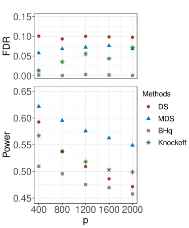
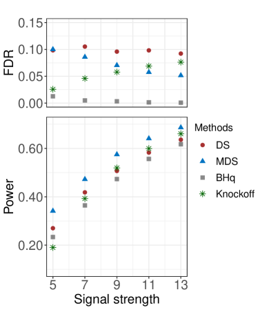
    Refer to caption
    Refer to caption
    Figure 7: Empirical FDRs and powers for linear models with a GWAS design matrix. The sample size is n=800๐‘›800n=800. The signal strength along the x๐‘ฅx-axis in the right panel shows multiples of 1/n1๐‘›1/\sqrt{n}. In the left panel, we fix the signal strength at 9 and vary the dimension p๐‘p. In the right panel, we fix the dimension at p=1200๐‘1200p=1200 and vary the signal strength. The number of relevant features is p1=70subscript๐‘170p_{1}=70 across all settings, and the designated FDR control level is q=0.1๐‘ž0.1q=0.1. Each dot in the figure represents the average from 50 independent runs.

We conclude this section with some remarks on the variance of the FDP. Note that DS and the knockoff filter rank features using the mirror statistics Mjsubscript๐‘€๐‘—M_{j}โ€™s and the statistics Wjsubscript๐‘Š๐‘—W_{j}โ€™s (see Section 3.2 in Candรจs etย al. (2018)), respectively. The statistic Wjsubscript๐‘Š๐‘—W_{j} enjoys a flip-sign property, that is, the signs of Wjsubscript๐‘Š๐‘—W_{j}โ€™s for jโˆˆS0๐‘—subscript๐‘†0j\in S_{0} are independent, thus the FDP of the knockoff filter fluctuates and concentrates around the FDR. For DS, the signs of the mirror statistics Mjsubscript๐‘€๐‘—M_{j}โ€™s for jโˆˆS0๐‘—subscript๐‘†0j\in S_{0} are dependent so the variance of the FDP can be a more concerning issue for DS. FDR control becomes less meaningful if the variance is unacceptably large. We empirically check the variances of the FDP for the four competing methods across the aforementioned simulation settings. The results are summarized in Figures 18, 20, 21, and 22 in Supplementary Materials. We observed that except for the cases where the knockoff filter appears overly conservative (e.g., see Figure 20), the variances of the FDP are comparable for DS and the knockoff filter. More interestingly, perhaps due to its de-randomized nature, MDS achieves a lower variance of the FDP than the knockoff filter in a majority of simulation settings.

4.2 Gaussian graphical model

We set the designated FDR control level at q=0.2๐‘ž0.2q=0.2 and consider two types of graphs:

  1. 1.

    Banded graph. The precision matrix ฮ›ฮ›\Lambda is constructed such that ฮปjโ€‹j=1subscript๐œ†๐‘—๐‘—1\lambda_{jj}=1, ฮปiโ€‹j=signโ€‹(a)โ‹…|a||iโˆ’j|/csubscript๐œ†๐‘–๐‘—โ‹…sign๐‘Žsuperscript๐‘Ž๐‘–๐‘—๐‘\lambda_{ij}=\text{sign}(a)\cdot|a|^{|i-j|/c} if 0<|iโˆ’j|โ‰คs0๐‘–๐‘—๐‘ 0<|i-j|\leq s, and ฮปiโ€‹j=0subscript๐œ†๐‘–๐‘—0\lambda_{ij}=0 if |iโˆ’j|>s๐‘–๐‘—๐‘ |i-j|>s. Throughout, we set c=1.5๐‘1.5c=1.5 following Li and Maathuis (2019). Other parameters including the sample size n๐‘›n, the dimension p๐‘p, the partial correlation (signal strength) a๐‘Ža, and the nodewise sparsity s๐‘ s will be specified case by case.

  2. 2.

    Blockwise diagonal graph. The precision matrix ฮ›ฮ›\Lambda is blockwise diagonal with equally sized squared blocks generated in the same fashion. Throughout, we fix the block size to be 25 ร—\times 25. In each block, all the diagonal elements are set to be 1, and the off-diagonal elements are independently drawn from the uniform distribution Unifโ€‹((โˆ’0.8,โˆ’0.4)โˆช(0.4,0.8))Unif0.80.40.40.8\text{Unif}((-0.8,-0.4)\cup(0.4,0.8)).

For both types of graphs, the precision matrix ฮ›ฮ›\Lambda generated from the aforementioned processes may not be positive definite. If ฮปminโ€‹(ฮ›)<0subscript๐œ†ฮ›0\lambda_{\min}(\Lambda)<0, we reset ฮ›โ†ฮ›+(ฮปminโ€‹(ฮ›)+0.005)โ€‹Ipโ†ฮ›ฮ›subscript๐œ†ฮ›0.005subscript๐ผ๐‘\Lambda\leftarrow\Lambda+(\lambda_{\min}(\Lambda)+0.005)I_{p} following Liu (2013). Three classes of competing methods are tested out, including (1) DS and MDS; (2) BHq; (3) GFC (Liu, 2013). For MDS, nodewisely, we replicate DS 50 times and aggregate the selection results using Algorithm 2. For BHq, the p-values are calculated based on the pairwise partial correlation test using the R package ppcor (Kim, 2015). For GFC, we use the R package SILGGM (Zhang etย al., 2018) to implement it.

For the banded graph, we test out the following four scenarios:

  1. ย ย ย (a)

    fix p=100๐‘100p=100, s=8๐‘ 8s=8, a=โˆ’0.6๐‘Ž0.6a=-0.6, and vary the sample size nโˆˆ{500,1000,1500,2000,2500}๐‘›5001000150020002500n\in\{500,1000,1500,2000,2500\};

  2. ย ย ย (b)

    fix n=1000๐‘›1000n=1000, s=8๐‘ 8s=8, a=โˆ’0.6๐‘Ž0.6a=-0.6, and vary the dimension pโˆˆ{50,100,150,200,250}๐‘50100150200250p\in\{50,100,150,200,250\};

  3. ย ย ย (c)

    fix n=1000๐‘›1000n=1000, p=100๐‘100p=100, a=โˆ’0.6๐‘Ž0.6a=-0.6, and vary the nodewise sparsity sโˆˆ{4,6,8,10,12}๐‘ 4681012s\in\{4,6,8,10,12\};

  4. ย ย ย (d)

    fix n=1000๐‘›1000n=1000, p=100๐‘100p=100, s=8๐‘ 8s=8, and vary the signal strength aโˆˆ{โˆ’0.5,โˆ’0.6,โˆ’0.7,โˆ’0.8,โˆ’0.9}๐‘Ž0.50.60.70.80.9a\in\{-0.5,-0.6,-0.7,-0.8,-0.9\}.

For the blockwise diagonal graph, we test out the following two scenarios:

  1. ย ย ย (a)

    fix p=100๐‘100p=100, and vary the sample size nโˆˆ{200,300,400,500,600}๐‘›200300400500600n\in\{200,300,400,500,600\};

  2. ย ย ย (b)

    fix n=500๐‘›500n=500, and vary the dimension pโˆˆ{50,100,150,200,250}๐‘50100150200250p\in\{50,100,150,200,250\}.

The results for the banded graphs and the blockwise diagonal graphs are summarized in Figures 8 and 9, respectively. We see that all the methods achieve FDR control at the designated level across different scenarios. For the banded graphs, DS and MDS are the two leading methods with significantly higher powers and also lower FDRs compared to the other two competing methods. GFC and BHq perform similarly, of which GFC has a slightly higher power when p๐‘p is large or the signal strength is strong. In panel (d) of Figure 8, the power of BHq exhibits an opposite trend compared to the other methods. One possible reason is that the pairwise correlation decreases when we increase a๐‘Ža from -0.9 to -0.5. Thus, the power of BHq increases as the p-values become less correlated. For the blockwise diagonal graphs, MDS performs the best across all scenarios, enjoying a higher power and also a lower FDR compared to DS. GFC performs similarly as DS in most scenarios, except for the case when p๐‘p is large, in which the power of GFC drops significantly.
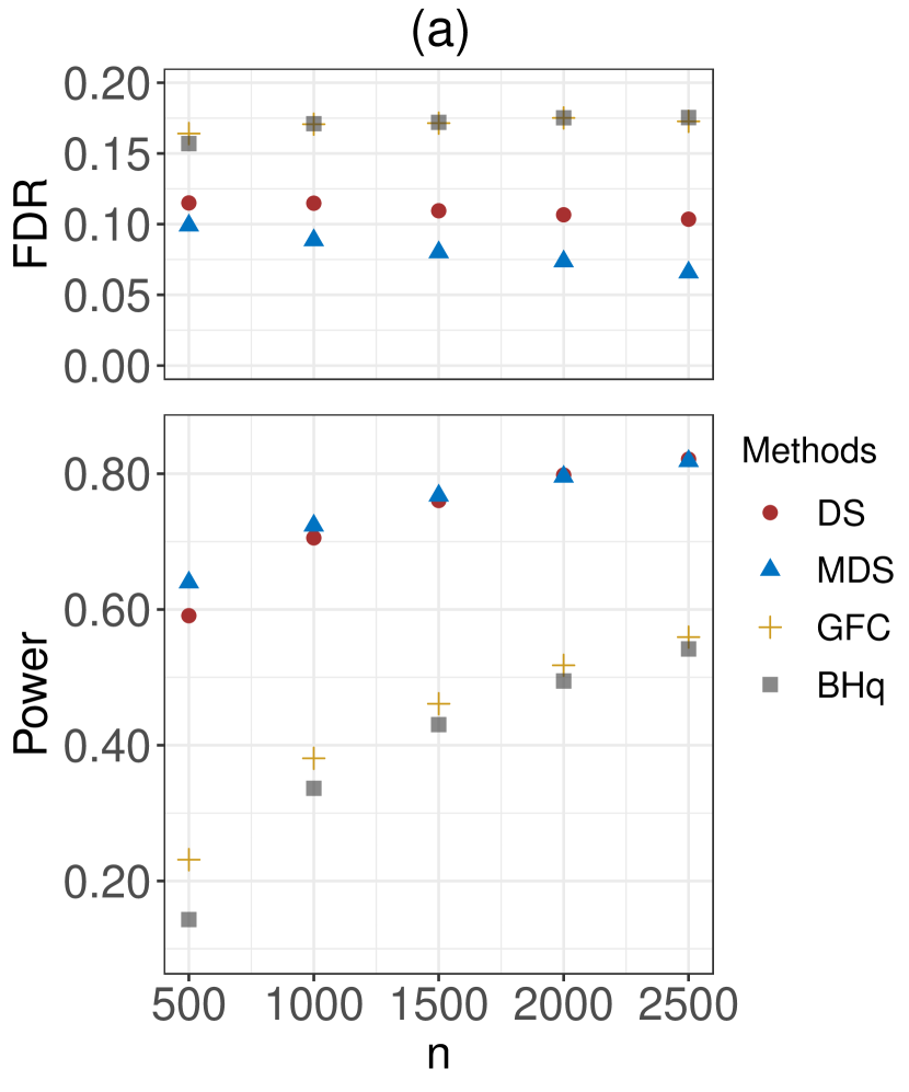
Refer to caption
Refer to caption
Refer to caption
Refer to caption
Figure 8: Empirical FDRs and powers for the banded graphs. The designated FDR control level is q=0.2๐‘ž0.2q=0.2. Each dot in the figure represents the average from 50 independent runs.
Refer to caption
Refer to caption
Figure 9: Empirical FDRs and powers for the blockwise diagonal graphs. The designated FDR control level is q=0.2๐‘ž0.2q=0.2. Each dot in the figure represents the average from 50 independent runs.

4.3 Real data application: HIV drug resistance

We apply DS and MDS to detect mutations in the Human Immunodeficiency Virus Type 1 (HIV-1) that are associated with drug resistance. The data set, which has also been analyzed in Rhee etย al. (2006), Barber and Candรจs (2015), and Lu etย al. (2018), contains resistance measurements of seven drugs for protease inhibitors (PIs), six drugs for nucleoside reverse-transcriptase inhibitors (NRTIs), and three drugs for nonnucleoside reverse transcriptase inhibitors (NNRTIs). We focus on the first two classes of inhibitors, PI and NRTI.

The response vector ๐’š๐’š\bm{y} calibrates the log-fold-increase of the lab-tested drug resistance. The design matrix ๐‘ฟ๐‘ฟ\bm{X} is binary, in which the j๐‘—j-th column indicates the presence or absence of the j๐‘—j-th mutation. The task is to select relevant mutations for each inhibitor against different drugs. The data is preprocessed as follows. First, we remove the patients with missing drug resistance information. Second, we exclude those mutations that appear fewer than three times across all patients. The sample size n๐‘›n and the number of mutations p๐‘p vary from drug to drug, but are all in hundreds with n/p๐‘›๐‘n/p ranging from 1.5 to 4 (see Figures 10 and 11). We assume a linear model between the response and features with no interactions.

Five methods are compared, including DeepPINK with the model-X knockoffs (Lu etย al., 2018), the fixed-design knockoff filter (Barber and Candรจs, 2015), BHq, DS, and MDS. For DeepPINK, the knockoff filter, and BHq, we report the selection results obtained in Lu etย al. (2018). The designated FDR control level is q=0.2๐‘ž0.2q=0.2 throughout. As in Barber and Candรจs (2015), we treat the existing treatment-selected mutation (TSM) panels (Rhee etย al., 2005) as the ground truth.

For PI, the number of discovered mutations for each drug, including the number of true and false positives, are summarized in Figure 10. We see that MDS performs the best for three out of seven PI drugs, including ATV, LPV and SQV. For drugs APV, IDV, and RTV, MDS is comparable to DeepPINK, and both perform better than the knockoff filter and BHq. For drug NFV, MDS and the knockoff filter are the two leading methods. Figure 11 shows the corresponding results for the NRTI drugs. Among the six NRTI drugs, MDS performs the best in four, including ABC, D4T, DDI, and X3TC. For drug AZT, MDS and the knockoff filter perform the best. For drug TDF, MDS is comparable to DeepPINK, and both are much better than BHq and the knockoff filter. In particular, we see that the knockoff filter has no power and does not select any mutations for drugs DDI, TDF, and X3TC.
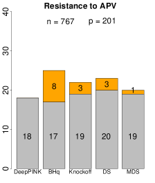
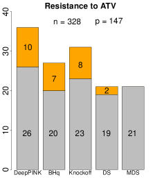
Refer to caption
Refer to caption
Refer to caption
Refer to caption
Refer to caption
Refer to caption
Refer to caption
Figure 10: Numbers of the discovered mutations for the seven PI drugs. The grey and orange bars represent the numbers of true and false positives, respectively. The designated FDR control level is q=0.2๐‘ž0.2q=0.2.
Refer to caption
Refer to caption
Refer to caption
Refer to caption
Refer to caption
Refer to caption
Figure 11: Numbers of the discovered mutations for the six NRTI drugs. The grey and orange bars represent the numbers of true and false positives, respectively. The designated FDR control level is q=0.2๐‘ž0.2q=0.2.

5 Concluding Remarks

We have described a general data-splitting framework to control the FDR for feature selection in high-dimensional regressions. We theoretically prove and empirically demonstrate that the proposed approaches (DS and MDS) allow us to asymptotically control the FDR in canonical statistical models including linear and Gaussian graphical models. MDS is shown to be a particularly attractive strategy as it helps stabilize the selection result and improves the power. Both DS and MDS require little knowledge on the joint distribution of features in consideration, and are conceptually simple and easy to implement based upon existing softwares for high-dimensional regression methods.

We conclude by pointing out several directions for future work. First, for linear models, an interesting extension of the Lasso + OLS procedure is to consider features with a group structure. A natural strategy is to substitute Lasso with group Lasso. However, unlike Lasso, group Lasso can potentially select more than n๐‘›n features (n๐‘›n is the sample size), thus the companion OLS step, which guarantees the symmetric assumption, may not be easily applied. Second, we would like to investigate the applicability and the theoretical properties of DS and MDS for dealing with neural networks and other nonlinear models, in order to handle more complex data such as images and natural languages. Third, it is of interest to investigate the multiple testing problem in sparse high-dimensional covariance matrix estimation, where some thresholding estimators are typically employed. Our proposed framework is applicable as long as the estimator of any zero covariance entry is symmetric about 0. Last but not the least, extensions of the data-splitting framework to handle data containing dependent observations or having hierarchical structures are of immediate interest.

Acknowledge

We thank Lucas Janson, Wenshuo Wang, and Dongming Huang for many helpful discussions and constructive suggestions. We also thank the three anonymous referees for their detailed critiques, especially the helpful comments on implementing the model-X knockoff filter. This research is supported in part by the National Science Foundation grants DMS-1903139 and DMS-2015411.

References

  • Azriel and Schwartzman (2015) Azriel, D. and A.ย Schwartzman (2015). The empirical distribution of a large number of correlated Normal variables. Journal of the American Statistical Associationย 110(511), 1217โ€“1228.
  • Barber and Candรจs (2015) Barber, R.ย F. and E.ย J. Candรจs (2015). Controlling the false discovery rate via knockoffs. The Annals of Statisticsย 43(5), 2055โ€“2085.
  • Barber and Candรจs (2019) Barber, R.ย F. and E.ย J. Candรจs (2019). A knockoff filter for high-dimensional selective inference. The Annals of Statisticsย 47(5), 2504โ€“2537.
  • Barber etย al. (2020) Barber, R.ย F., E.ย J. Candรจs, and R.ย J. Samworth (2020). Robust inference with knockoffs. The Annals of Statisticsย 48(3), 1409โ€“1431.
  • Bates etย al. (2020) Bates, S., E.ย J. Candรฉs, L.ย Janson, and W.ย Wang (2020). Metropolized knockoff sampling. Journal of the American Statistical Association.
  • Benjamini and Gavrilov (2009) Benjamini, Y. and Y.ย Gavrilov (2009). A simple forward selection procedure based on false discovery rate control. The Annals of Applied Statisticsย 3(1), 179โ€“198.
  • Benjamini and Hochberg (1995) Benjamini, Y. and Y.ย Hochberg (1995). Controlling the false discovery rate: a practical and powerful approach to multiple testing. Journal of the Royal Statistical Society: Series B (Statistical Methodology)ย 57(1), 289โ€“300.
  • Benjamini and Yekutieli (2001) Benjamini, Y. and D.ย Yekutieli (2001). The control of the false discovery rate in multiple testing under dependency. The Annals of Statisticsย 29(4), 1165โ€“1188.
  • Bickel etย al. (2009) Bickel, P.ย J., Y.ย Ritov, and A.ย B. Tsybakov (2009). Simultaneous analysis of Lasso and Dantzig selector. The Annals of Statisticsย 37(4), 1705โ€“1732.
  • Bogdan etย al. (2015) Bogdan, M., E.ย Berg, C.ย Sabatti, W.ย Su, and E.ย J. Candรจs (2015). Slope โ€“ adaptive variable selection via convex optimization. The Annals of Applied Statisticsย 9(3), 1103โ€“1150.
  • Candรจs etย al. (2018) Candรจs, E.ย J., Y.ย Fan, L.ย Janson, and J.ย Lv (2018). Panning for gold: โ€˜model-Xโ€™ knockoffs for high dimensional controlled variable selection. Journal of the Royal Statistical Society: Series B (Statistical Methodology)ย 80(3), 551โ€“577.
  • Clarke and Hall (2009) Clarke, S. and P.ย Hall (2009). Robustness of multiple testing procedures against dependence. The Annals of Statisticsย 37(1), 332โ€“358.
  • Cox (1975) Cox, D.ย R. (1975). A note on data-splitting for the evaluation of significance levels. Biometrikaย 62(2), 441โ€“444.
  • Dai etย al. (2020) Dai, C., B.ย Lin, X.ย Xing, and J.ย S. Liu (2020). A scale-free approach for false discovery rate control in generalized linear models. arXiv preprint: 2007.01237.
  • Dezeure etย al. (2015) Dezeure, R., P.ย Bรผhlmann, L.ย Meier, and N.ย Meinshausen (2015). High-dimensional inference: confidence intervals, p-values and R-software hdi. Statistical Science, 533โ€“558.
  • Efron (2005) Efron, B. (2005). Local false discovery rates. Technical report.
  • Efron etย al. (2001) Efron, B., R.ย Tibshirani, J.ย D. Storey, and V.ย Tusher (2001). Empirical Bayes analysis of a microarray experiment. Journal of the American Statistical Associationย 96(456), 1151โ€“1160.
  • Efroymson (1960) Efroymson, M. (1960). Multiple regression analysis. Mathematical Methods for Digital Computers, 191โ€“203.
  • Fan etย al. (2020) Fan, Y., E.ย Demirkaya, G.ย Li, and J.ย Lv (2020). Rank: large-scale inference with graphical nonlinear knockoffs. Journal of the American Statistical Associationย 115(529), 362โ€“379.
  • Hoffman etย al. (2020) Hoffman, J.ย A., B.ย N. Papas, K.ย W. Trotter, and T.ย K. Archer (2020). Single-cell RNA sequencing reveals a heterogeneous response to glucocorticoids in breast cancer cells. Communications Biologyย 3(1), 1โ€“11.
  • Huang and Janson (2020) Huang, D. and L.ย Janson (2020). Relaxing the assumptions of knockoffs by conditioning. The Annals of Statisticsย 48(5), 3021โ€“3042.
  • Ignatiadis etย al. (2016) Ignatiadis, N., B.ย Klaus, J.ย B. Zaugg, and W.ย Huber (2016). Data-driven hypothesis weighting increases detection power in genome-scale multiple testing. Nature Methodsย 13(7), 577.
  • Javanmard and Javadi (2019) Javanmard, A. and H.ย Javadi (2019). False discovery rate control via debiased Lasso. Electronic Journal of Statisticsย 13(1), 1212โ€“1253.
  • Javanmard and Montanari (2014) Javanmard, A. and A.ย Montanari (2014). Confidence intervals and hypothesis testing for high-dimensional regression. The Journal of Machine Learning Researchย 15(1), 2869โ€“2909.
  • Jordon etย al. (2019) Jordon, J., J.ย Yoon, and M.ย V.ย D. Schaar (2019). KnockoffGAN: generating knockoffs for feature selection using generative adversarial networks. The International Conference on Learning Representations.
  • Katsevich and Sabatti (2019) Katsevich, E. and C.ย Sabatti (2019). Multilayer knockoff filter: controlled variable selection at multiple resolutions. The Annals of Applied Statisticsย 13(1), 1โ€“33.
  • Ke etย al. (2020) Ke, Z.ย T., J.ย S. Liu, and Y.ย Ma (2020). Power of FDR control methods: the impact of ranking algorithm, tampered design, and symmetric statistic. arXiv preprint: 2010.08132.
  • Kim (2015) Kim, S. (2015). ppcor: an R package for a fast calculation to semi-partial correlation coefficients. Communications for Statistical Applications and Methodsย 22(6), 665.
  • Kotz etย al. (2000) Kotz, S., N.ย Balakrishnan, and N.ย L. Johnson (2000). Bivariate and trivariate Normal distributions. Continuous Multivariate Distributionsย 1, 251โ€“348.
  • Lauritzen (1996) Lauritzen, S.ย L. (1996). Graphical models.
  • Lee etย al. (2016) Lee, J.ย D., D.ย L. Sun, Y.ย Sun, and J.ย E. Taylor (2016). Exact post-selection inference, with application to the Lasso. The Annals of Statisticsย 44(3), 907โ€“927.
  • Li and Maathuis (2019) Li, J. and M.ย H. Maathuis (2019). Nodewise knockoffs: false discovery rate control for Gaussian graphical models. arXiv preprint: 1908.11611.
  • Liu and Rigollet (2019) Liu, J. and P.ย Rigollet (2019). Power analysis of knockoff filters for correlated designs. Advances in Neural Information Processing Systems 32, 15446โ€“15455.
  • Liu (2013) Liu, W. (2013). Gaussian graphical model estimation with false discovery rate control. The Annals of Statisticsย 41(6), 2948โ€“2978.
  • Lu etย al. (2018) Lu, Y., Y.ย Fan, J.ย Lv, and W.ย S. Noble (2018). DeepPINK: reproducible feature selection in deep neural networks. Advances in Neural Information Processing Systems, 8676โ€“8686.
  • Ma etย al. (2020) Ma, R., T.ย T. Cai, and H.ย Li (2020). Global and simultaneous hypothesis testing for high-dimensional Logistic regression models. Journal of the American Statistical Association, 1โ€“15.
  • Meinshausen and Bรผhlmann (2006) Meinshausen, N. and P.ย Bรผhlmann (2006). High-dimensional graphs and variable selection with the Lasso. The Annals of Statisticsย 34(3), 1436โ€“1462.
  • Meinshausen and Bรผhlmann (2010) Meinshausen, N. and P.ย Bรผhlmann (2010). Stability selection. Journal of the Royal Statistical Society: Series B (Statistical Methodology)ย 72(4), 417โ€“473.
  • Meinshausen etย al. (2009) Meinshausen, N., L.ย Meier, and P.ย Bรผhlmann (2009). p-values for high-dimensional regression. Journal of the American Statistical Associationย 104(488), 1671โ€“1681.
  • Meinshausen and Yu (2009) Meinshausen, N. and B.ย Yu (2009). Lasso-type recovery of sparse representations for high-dimensional data. The Annals of Statisticsย 37(1), 246โ€“270.
  • Moran (1973) Moran, P. A.ย P. (1973). Dividing a sample into two parts a statistical dilemma. Sankhyฤ: The Indian Journal of Statistics, Series A, 329โ€“333.
  • Oโ€™Hara etย al. (2009) Oโ€™Hara, R.ย B., M.ย J. Sillanpรครค, etย al. (2009). A review of Bayesian variable selection methods: what, how and which. Bayesian Analysisย 4(1), 85โ€“117.
  • Raskutti etย al. (2010) Raskutti, G., M.ย J. Wainwright, and B.ย Yu (2010). Restricted eigenvalue properties for correlated Gaussian designs. Journal of Machine Learning Researchย 11(8), 2241โ€“2259.
  • Rhee etย al. (2005) Rhee, S.ย Y., W.ย J. Fessel, A.ย R. Zolopa, L.ย Hurley, T.ย Liu, J.ย Taylor, D.ย P. Nguyen, S.ย Slome, D.ย Klein, and M.ย Horberg (2005). HIV-1 protease and reverse-transcriptase mutations: correlations with antiretroviral therapy in subtype B isolates and implications for drug-resistance surveillance. The Journal of Infectious Diseasesย 192(3), 456โ€“465.
  • Rhee etย al. (2006) Rhee, S.ย Y., J.ย Taylor, G.ย Wadhera, A.ย Ben-Hur, D.ย L. Brutlag, and R.ย W. Shafer (2006). Genotypic predictors of human immunodeficiency virus type 1 drug resistance. Proceedings of the National Academy of Sciencesย 103(46), 17355โ€“17360.
  • Romano and DiCiccio (2019) Romano, J.ย P. and C.ย DiCiccio (2019). Multiple data splitting for testing.
  • Romano etย al. (2019) Romano, Y., M.ย Sesia, and E.ย J. Candรจs (2019). Deep knockoffs. Journal of the American Statistical Association.
  • Rubin etย al. (2006) Rubin, D., S.ย Dudoit, and M.ย V. der Laan (2006). A method to increase the power of multiple testing procedures through sample splitting. Statistical Applications in Genetics and Molecular Biologyย 5(1).
  • Rudelson and Zhou (2013) Rudelson, M. and S.ย Zhou (2013). Reconstruction from anisotropic random measurements. IEEE Transactions on Information Theoryย 59(6), 3434โ€“3447.
  • Sarkar (2002) Sarkar, S.ย K. (2002). Some results on false discovery rate in stepwise multiple testing procedures. The Annals of Statisticsย 30(1), 239โ€“257.
  • Sesia etย al. (2020) Sesia, M., E.ย Katsevich, S.ย Bates, E.ย J. Candรจs, and C.ย Sabatti (2020). Multi-resolution localization of causal variants across the genome. Nature Communicationsย 11(1).
  • Sesia etย al. (2018) Sesia, M., C.ย Sabatti, and E.ย J. Candรจs (2018). Gene hunting with hidden Markov model knockoffs. Biometrikaย 106(1), 1โ€“18.
  • Stone (1974) Stone, M. (1974). Cross-validatory choice and assessment of statistical predictions. Journal of the Royal Statistical Society: Series B (Statistical Methodology)ย 36(2), 111โ€“133.
  • Storey (2003) Storey, J.ย D. (2003). The positive false discovery rate: a Bayesian interpretation and the q-value. The Annals of Statisticsย 31(6), 2013โ€“2035.
  • Storey etย al. (2004) Storey, J.ย D., J.ย E. Taylor, and D.ย Siegmund (2004). Strong control, conservative point estimation and simultaneous conservative consistency of false discovery rates: a unified approach. Journal of the Royal Statistical Society: Series B (Statistical Methodology)ย 66(1), 187โ€“205.
  • Tibshirani (1996) Tibshirani, R. (1996). Regression shrinkage and selection via the Lasso. Journal of the Royal Statistical Society: Series B (Statistical Methodology)ย 58(1), 267โ€“288.
  • Tibshirani etย al. (2016) Tibshirani, R.ย J., J.ย Taylor, R.ย Lockhart, and R.ย Tibshirani (2016). Exact post-selection inference for sequential regression procedures. Journal of the American Statistical Associationย 111(514), 600โ€“620.
  • Vanย de Geer and Bรผhlmann (2009) Vanย de Geer, S.ย A. and P.ย Bรผhlmann (2009). On the conditions used to prove oracle results for the lasso. Electron. J. Statist.ย 3, 1360โ€“1392.
  • Van de Geer etย al. (2014) Van de Geer, S.ย A., P.ย Bรผhlmann, Y.ย Ritov, and R.ย Dezeure (2014). On asymptotically optimal confidence regions and tests for high-dimensional models. The Annals of Statisticsย 42(3), 1166โ€“1202.
  • vanย de Wiel etย al. (2009) vanย de Wiel, M.ย A., J.ย Berkhof, and W.ย N. van Wieringen (2009). Testing the prediction error difference between two predictors. Biostatisticsย 10(3), 550โ€“560.
  • Wainwright (2019) Wainwright, M.ย J. (2019). High-dimensional statistics: a non-asymptotic viewpoint, Volumeย 48. Cambridge University Press.
  • Wang and Janson (2020) Wang, W. and L.ย Janson (2020). A power analysis of the conditional randomization test and knockoffs. arXiv preprint: 2010.02304.
  • Wasserman and Roeder (2009) Wasserman, L. and K.ย Roeder (2009). High dimensional variable selection. The Annals of Statisticsย 37(5A), 2178.
  • Weinstein etย al. (2017) Weinstein, A., R.ย F. Barber, and E.ย J. Candรจs (2017). A power and prediction analysis for knockoffs with Lasso statistics.
  • Weinstein etย al. (2020) Weinstein, A., W.ย J. Su, M.ย Bogdan, R.ย F. Barber, and E.ย J. Candรจs (2020). A power analysis for knockoffs with the Lasso coefficient-difference statistic.
  • Wu (2008) Wu, W.ย B. (2008). On false discovery control under dependence. The Annals of Statisticsย 36, 364โ€“โ€“380.
  • Xing etย al. (2019) Xing, X., Z.ย Zhao, and J.ย S. Liu (2019). Controlling false discovery rate using Gaussian mirrors. arXiv preprint: 1911.09761.
  • Zhang and Zhang (2014) Zhang, C.ย H. and S.ย S. Zhang (2014). Confidence intervals for low dimensional parameters in high dimensional linear models. Journal of the Royal Statistical Society: Series B (Statistical Methodology)ย 76(1), 217โ€“242.
  • Zhang etย al. (2018) Zhang, R., Z.ย Ren, and W.ย Chen (2018). SILGGM: an extensive R package for efficient statistical inference in large-scale gene networks. PLoS Computational Biologyย 14(8).

6 Supplementary Materials

6.1 Proofs

Throughout, we consider the general form of the mirror statistic defined in (1), in which function fโ€‹(u,v)๐‘“๐‘ข๐‘ฃf(u,v) is non-negative, symmetric about u๐‘ขu and v๐‘ฃv, and monotonically increasing in both u๐‘ขu and v๐‘ฃv. For any t>0๐‘ก0t>0 and uโ‰ฅ0๐‘ข0u\geq 0, let

โ„tโ€‹(u)=inf{vโ‰ฅ0:fโ€‹(u,v)>t}subscriptโ„๐‘ก๐‘ขinfimumconditional-set๐‘ฃ0๐‘“๐‘ข๐‘ฃ๐‘ก\mathcal{I}_{t}(u)=\inf\{v\geq 0:f(u,v)>t\}

with the convention infโˆ…=+โˆžinfimum\inf\varnothing=+\infty. The CDF and pdf of the standard Normal distribution are denoted as ฮฆฮฆ\Phi and ฯ•italic-ฯ•\phi, respectively.

6.1.1 Proof of Proposition 1

Let Z1,Z2subscript๐‘1subscript๐‘2Z_{1},Z_{2} follow Nโ€‹(0,1)๐‘01N(0,1), Z3,Z4subscript๐‘3subscript๐‘4Z_{3},Z_{4} follow Nโ€‹(ฯ‰,1)๐‘๐œ”1N(\omega,1), all of which are independent. Without loss of generality, we assume that the designated FDR control level qโˆˆ(0,1)๐‘ž01q\in(0,1) satisfies rโ€‹q/(1โˆ’q)<1๐‘Ÿ๐‘ž1๐‘ž1rq/(1-q)<1, otherwise selecting all features would maximize the power and also achieve asymptotic FDR control. Let foptโ€‹(u,v)superscript๐‘“opt๐‘ข๐‘ฃf^{\text{opt}}(u,v) be the optimal choice, and let S^optsuperscript^๐‘†opt\widehat{S}^{\text{opt}} be the optimal selection result that achieves asymptotic FDR control. By the law of large numbers, we have

limpโ†’โˆž#โ€‹{j:jโˆˆS0,jโˆˆS^opt}#โ€‹{j:jโˆˆS^opt}=โ„™โ€‹(jโˆˆS^optโˆฃjโˆˆS0)โ„™โ€‹(jโˆˆS^optโˆฃjโˆˆS0)+rโ€‹โ„™โ€‹(jโˆˆS^optโˆฃjโˆˆS1)โ‰คq,subscriptโ†’๐‘#conditional-set๐‘—formulae-sequence๐‘—subscript๐‘†0๐‘—superscript^๐‘†opt#conditional-set๐‘—๐‘—superscript^๐‘†optโ„™๐‘—conditionalsuperscript^๐‘†opt๐‘—subscript๐‘†0โ„™๐‘—conditionalsuperscript^๐‘†opt๐‘—subscript๐‘†0๐‘Ÿโ„™๐‘—conditionalsuperscript^๐‘†opt๐‘—subscript๐‘†1๐‘ž\lim_{p\to\infty}\frac{\#\{j:j\in S_{0},j\in\widehat{S}^{\text{opt}}\}}{\#\{j:j\in\widehat{S}^{\text{opt}}\}}=\frac{\mathbbm{P}(j\in\widehat{S}^{\text{opt}}\mid j\in S_{0})}{\mathbbm{P}(j\in\widehat{S}^{\text{opt}}\mid j\in S_{0})+r\mathbbm{P}(j\in\widehat{S}^{\text{opt}}\mid j\in S_{1})}\leq q, (8)

in which the numerator is the type-I error. More precisely,

โ„™โ€‹(jโˆˆS^optโˆฃjโˆˆS0)=โ„™โ€‹(signโ€‹(Z1โ€‹Z2)โ€‹foptโ€‹(|Z1|,|Z2|)>topt),โ„™๐‘—conditionalsuperscript^๐‘†opt๐‘—subscript๐‘†0โ„™signsubscript๐‘1subscript๐‘2superscript๐‘“optsubscript๐‘1subscript๐‘2superscript๐‘กopt\displaystyle\mathbbm{P}(j\in\widehat{S}^{\text{opt}}\mid j\in S_{0})=\mathbbm{P}(\text{sign}(Z_{1}Z_{2})f^{\text{opt}}(|Z_{1}|,|Z_{2}|)>t^{\text{opt}}),
โ„™โ€‹(jโˆˆS^optโˆฃjโˆˆS1)=โ„™โ€‹(signโ€‹(Z3โ€‹Z4)โ€‹foptโ€‹(|Z3|,|Z4|)>topt).โ„™๐‘—conditionalsuperscript^๐‘†opt๐‘—subscript๐‘†1โ„™signsubscript๐‘3subscript๐‘4superscript๐‘“optsubscript๐‘3subscript๐‘4superscript๐‘กopt\displaystyle\mathbbm{P}(j\in\widehat{S}^{\text{opt}}\mid j\in S_{1})=\mathbbm{P}(\text{sign}(Z_{3}Z_{4})f^{\text{opt}}(|Z_{3}|,|Z_{4}|)>t^{\text{opt}}).

topt>0superscript๐‘กopt0t^{\text{opt}}>0 is the cutoff that maximizes the power โ„™โ€‹(jโˆˆS^optโˆฃjโˆˆS1)โ„™๐‘—conditionalsuperscript^๐‘†opt๐‘—subscript๐‘†1\mathbbm{P}(j\in\widehat{S}^{\text{opt}}\mid j\in S_{1}), under the constraint that Equation (8) holds.

We now consider testing whether Xjsubscript๐‘‹๐‘—X_{j} is a null feature, with the significance level ฮฑ๐›ผ\alpha specified as:

ฮฑ=rโ€‹q1โˆ’qโ€‹โ„™โ€‹(jโˆˆS^optโˆฃjโˆˆS1)<1.๐›ผ๐‘Ÿ๐‘ž1๐‘žโ„™๐‘—conditionalsuperscript^๐‘†opt๐‘—subscript๐‘†11\alpha=\frac{rq}{1-q}\mathbbm{P}(j\in\widehat{S}^{\text{opt}}\mid j\in S_{1})<1.

We have two observations ฮฒ^j(1)superscriptsubscript^๐›ฝ๐‘—1\widehat{\beta}_{j}^{(1)} and ฮฒ^j(2)superscriptsubscript^๐›ฝ๐‘—2\widehat{\beta}_{j}^{(2)}, which independently follow Nโ€‹(0,1)๐‘01N(0,1) or Nโ€‹(ฯ‰,1)๐‘๐œ”1N(\omega,1) if Xjsubscript๐‘‹๐‘—X_{j} is a null feature or a relevant feature, respectively. By Equation (8), the test which rejects the null hypothesis (i.e., jโˆˆS^opt๐‘—superscript^๐‘†optj\in\widehat{S}^{\text{opt}}) if

signโ€‹(ฮฒ^j(1)โ€‹ฮฒ^j(2))โ€‹foptโ€‹(|ฮฒ^j(1)|,|ฮฒ^j(2)|)>toptsignsuperscriptsubscript^๐›ฝ๐‘—1superscriptsubscript^๐›ฝ๐‘—2superscript๐‘“optsuperscriptsubscript^๐›ฝ๐‘—1superscriptsubscript^๐›ฝ๐‘—2superscript๐‘กopt\text{sign}(\widehat{\beta}_{j}^{(1)}\widehat{\beta}_{j}^{(2)})f^{\text{opt}}(|\widehat{\beta}_{j}^{(1)}|,|\widehat{\beta}_{j}^{(2)}|)>t^{\text{opt}}

achieves the significance level ฮฑ๐›ผ\alpha.

In the following, f๐‘“f refers to fโ€‹(u,v)=u+v๐‘“๐‘ข๐‘ฃ๐‘ข๐‘ฃf(u,v)=u+v. We consider the following rejection rule,

signโ€‹(ฮฒ^j(1)โ€‹ฮฒ^j(2))โ€‹fโ€‹(|ฮฒ^j(1)|,|ฮฒ^j(2)|)>tlik,signsuperscriptsubscript^๐›ฝ๐‘—1superscriptsubscript^๐›ฝ๐‘—2๐‘“superscriptsubscript^๐›ฝ๐‘—1superscriptsubscript^๐›ฝ๐‘—2superscript๐‘กlik\text{sign}(\widehat{\beta}_{j}^{(1)}\widehat{\beta}_{j}^{(2)})f(|\widehat{\beta}_{j}^{(1)}|,|\widehat{\beta}_{j}^{(2)}|)>t^{\text{lik}},

in which tlik>0superscript๐‘กlik0t^{\text{lik}}>0 satisfies

โ„™โ€‹(fโ€‹(|Z1|,|Z2|)>tlikโˆฃsignโ€‹(Z1)=signโ€‹(Z2))=2โ€‹ฮฑ.โ„™๐‘“subscript๐‘1subscript๐‘2conditionalsuperscript๐‘กliksignsubscript๐‘1signsubscript๐‘22๐›ผ\mathbbm{P}(f(|Z_{1}|,|Z_{2}|)>t^{\text{lik}}\mid\text{sign}(Z_{1})=\text{sign}(Z_{2}))=2\alpha. (9)

Let S^liksuperscript^๐‘†lik\widehat{S}^{\text{lik}} be the corresponding selection set. We first show that this rejection rule controls the type-I error below ฮฑ๐›ผ\alpha. Indeed,

โ„™(jโˆˆS^likโˆฃjโˆˆS0)=12โ„™(f(|ฮฒ^j(1)|,|ฮฒ^j(2)|)>tlikโˆฃjโˆˆS0,sign(ฮฒ^j(1))=sign(ฮฒ^j(2)))=ฮฑ.\displaystyle\mathbbm{P}(j\in\widehat{S}^{\text{lik}}\mid j\in S_{0})=\frac{1}{2}\mathbbm{P}(f(|\widehat{\beta}_{j}^{(1)}|,|\widehat{\beta}_{j}^{(2)}|)>t^{\text{lik}}\mid j\in S_{0},\ \text{sign}(\widehat{\beta}_{j}^{(1)})=\text{sign}(\widehat{\beta}_{j}^{(2)}))=\alpha. (10)

In terms of power, we have

โ„™โ€‹(jโˆˆS^likโˆฃjโˆˆS1)โ„™๐‘—conditionalsuperscript^๐‘†lik๐‘—subscript๐‘†1\displaystyle\mathbbm{P}(j\in\widehat{S}^{\text{lik}}\mid j\in S_{1}) =pwโ„™(f(|ฮฒ^j(1)|,|ฮฒ^j(2)|)>tlikโˆฃjโˆˆS1,sign(ฮฒ^j(1))=sign(ฮฒ^j(2)))\displaystyle=p_{w}\mathbbm{P}(f(|\widehat{\beta}_{j}^{(1)}|,|\widehat{\beta}_{j}^{(2)}|)>t^{\text{lik}}\mid j\in S_{1},\ \text{sign}(\widehat{\beta}_{j}^{(1)})=\text{sign}(\widehat{\beta}_{j}^{(2)})) (11)
โ‰ฅpwโ„™(fopt(|ฮฒ^j(1)|,|ฮฒ^j(2)|)>toptโˆฃjโˆˆS1,sign(ฮฒ^j(1))=sign(ฮฒ^j(2)))\displaystyle\geq p_{w}\mathbbm{P}(f^{\text{opt}}(|\widehat{\beta}_{j}^{(1)}|,|\widehat{\beta}_{j}^{(2)}|)>t^{\text{opt}}\mid j\in S_{1},\ \text{sign}(\widehat{\beta}_{j}^{(1)})=\text{sign}(\widehat{\beta}_{j}^{(2)}))
=โ„™โ€‹(jโˆˆS^optโˆฃjโˆˆS1),absentโ„™๐‘—conditionalsuperscript^๐‘†opt๐‘—subscript๐‘†1\displaystyle=\mathbbm{P}(j\in\widehat{S}^{\text{opt}}\mid j\in S_{1}),

in which pw=โ„™โ€‹(signโ€‹(ฮฒ^j(1))=signโ€‹(ฮฒ^j(2))โˆฃjโˆˆS1)subscript๐‘๐‘คโ„™signsuperscriptsubscript^๐›ฝ๐‘—1conditionalsignsuperscriptsubscript^๐›ฝ๐‘—2๐‘—subscript๐‘†1p_{w}=\mathbbm{P}(\text{sign}(\widehat{\beta}_{j}^{(1)})=\text{sign}(\widehat{\beta}_{j}^{(2)})\mid j\in S_{1}). The inequality in the second line is a direct consequence of the Neymann-Pearson lemma.

To see this, suppose we only observe |ฮฒ^j(1)|,|ฮฒ^j(2)|superscriptsubscript^๐›ฝ๐‘—1superscriptsubscript^๐›ฝ๐‘—2|\widehat{\beta}_{j}^{(1)}|,|\widehat{\beta}_{j}^{(2)}| and also know that signโ€‹(ฮฒ^j(1))=signโ€‹(ฮฒ^j(2))signsuperscriptsubscript^๐›ฝ๐‘—1signsuperscriptsubscript^๐›ฝ๐‘—2\text{sign}(\widehat{\beta}_{j}^{(1)})=\text{sign}(\widehat{\beta}_{j}^{(2)}). Then the rejection rule fโ€‹(|ฮฒ^j(1)|,|ฮฒ^j(2)|)>tlik๐‘“superscriptsubscript^๐›ฝ๐‘—1superscriptsubscript^๐›ฝ๐‘—2superscript๐‘กlikf(|\widehat{\beta}_{j}^{(1)}|,|\widehat{\beta}_{j}^{(2)}|)>t^{\text{lik}} controls the type-I error below 2โ€‹ฮฑ2๐›ผ2\alpha by the definition of tliksuperscript๐‘กlikt^{\text{lik}} in (9). Further, the rejection rule fโ€‹(|ฮฒ^j(1)|,|ฮฒ^j(2)|)>topt๐‘“superscriptsubscript^๐›ฝ๐‘—1superscriptsubscript^๐›ฝ๐‘—2superscript๐‘กoptf(|\widehat{\beta}_{j}^{(1)}|,|\widehat{\beta}_{j}^{(2)}|)>t^{\text{opt}} also controls the type-I error below 2โ€‹ฮฑ2๐›ผ2\alpha by Equation (8). The likelihood ratio (LR) is given by

LR=ฯ•1โ€‹(|ฮฒ^j(1)|,|ฮฒ^j(2)|)ฯ•0โ€‹(|ฮฒ^j(1)|,|ฮฒ^j(2)|)โˆcoshโก(wโ€‹(ฮฒ^j(1)+ฮฒ^j(2))),LRsubscriptitalic-ฯ•1superscriptsubscript^๐›ฝ๐‘—1superscriptsubscript^๐›ฝ๐‘—2subscriptitalic-ฯ•0superscriptsubscript^๐›ฝ๐‘—1superscriptsubscript^๐›ฝ๐‘—2proportional-to๐‘คsuperscriptsubscript^๐›ฝ๐‘—1superscriptsubscript^๐›ฝ๐‘—2\text{LR}=\frac{\phi_{1}(|\widehat{\beta}_{j}^{(1)}|,|\widehat{\beta}_{j}^{(2)}|)}{\phi_{0}(|\widehat{\beta}_{j}^{(1)}|,|\widehat{\beta}_{j}^{(2)}|)}\propto\cosh(w(\widehat{\beta}_{j}^{(1)}+\widehat{\beta}_{j}^{(2)})),

where ฯ•1subscriptitalic-ฯ•1\phi_{1} and ฯ•0subscriptitalic-ฯ•0\phi_{0} are the joint densities of (Z3,Z4)subscript๐‘3subscript๐‘4(Z_{3},Z_{4}) and (Z1,Z2)subscript๐‘1subscript๐‘2(Z_{1},Z_{2}), respectively, conditioning on signโ€‹(Z1)=signโ€‹(Z2)signsubscript๐‘1signsubscript๐‘2\text{sign}(Z_{1})=\text{sign}(Z_{2}) and signโ€‹(Z3)=signโ€‹(Z4)signsubscript๐‘3signsubscript๐‘4\text{sign}(Z_{3})=\text{sign}(Z_{4}). Note that this is a monotone function of |ฮฒ^j(1)+ฮฒ^j(2)|superscriptsubscript^๐›ฝ๐‘—1superscriptsubscript^๐›ฝ๐‘—2|\widehat{\beta}_{j}^{(1)}+\widehat{\beta}_{j}^{(2)}|, which equals to |ฮฒ^j(1)|+|ฮฒ^j(2)|superscriptsubscript^๐›ฝ๐‘—1superscriptsubscript^๐›ฝ๐‘—2|\widehat{\beta}_{j}^{(1)}|+|\widehat{\beta}_{j}^{(2)}| under the condition signโ€‹(ฮฒ^j(1))=signโ€‹(ฮฒ^j(2))signsuperscriptsubscript^๐›ฝ๐‘—1signsuperscriptsubscript^๐›ฝ๐‘—2\text{sign}(\widehat{\beta}_{j}^{(1)})=\text{sign}(\widehat{\beta}_{j}^{(2)}).

Combining Equations (10) and (11), it follows that the selection set S^liksuperscript^๐‘†lik\widehat{S}^{\text{lik}} achieves asymptotic FDR control since

limpโ†’โˆž#โ€‹{j:jโˆˆS0,jโˆˆS^lik}#โ€‹{j:jโˆˆS^lik}subscriptโ†’๐‘#conditional-set๐‘—formulae-sequence๐‘—subscript๐‘†0๐‘—superscript^๐‘†lik#conditional-set๐‘—๐‘—superscript^๐‘†lik\displaystyle\lim_{p\to\infty}\frac{\#\{j:j\in S_{0},j\in\widehat{S}^{\text{lik}}\}}{\#\{j:j\in\widehat{S}^{\text{lik}}\}} =โ„™โ€‹(jโˆˆS^likโˆฃjโˆˆS0)โ„™โ€‹(jโˆˆS^likโˆฃjโˆˆS0)+rโ€‹โ„™โ€‹(jโˆˆS^likโˆฃjโˆˆS1)โ‰คq.absentโ„™๐‘—conditionalsuperscript^๐‘†lik๐‘—subscript๐‘†0โ„™๐‘—conditionalsuperscript^๐‘†lik๐‘—subscript๐‘†0๐‘Ÿโ„™๐‘—conditionalsuperscript^๐‘†lik๐‘—subscript๐‘†1๐‘ž\displaystyle=\frac{\mathbbm{P}(j\in\widehat{S}^{\text{lik}}\mid j\in S_{0})}{\mathbbm{P}(j\in\widehat{S}^{\text{lik}}\mid j\in S_{0})+r\mathbbm{P}(j\in\widehat{S}^{\text{lik}}\mid j\in S_{1})}\leq q.

As foptsuperscript๐‘“optf^{\text{opt}} is optimal, by Equation (11), fliksuperscript๐‘“likf^{\text{lik}} is also optimal. This concludes the proof of Proposition 1.

6.1.2 Proof of Proposition 2

For the ease of presentation, we introduce the following notations. For tโˆˆโ„๐‘กโ„t\in\mathbbm{R}, denote

G^p0โ€‹(t)=1p0โ€‹โˆ‘jโˆˆS0๐Ÿ™โ€‹(Mj>t),Gp0โ€‹(t)=1p0โ€‹โˆ‘jโˆˆS0โ„™โ€‹(Mj>t),formulae-sequencesubscriptsuperscript^๐บ0๐‘๐‘ก1subscript๐‘0subscript๐‘—subscript๐‘†01subscript๐‘€๐‘—๐‘กsubscriptsuperscript๐บ0๐‘๐‘ก1subscript๐‘0subscript๐‘—subscript๐‘†0โ„™subscript๐‘€๐‘—๐‘ก\displaystyle\widehat{G}^{0}_{p}(t)=\frac{1}{p_{0}}\sum_{j\in S_{0}}\mathbbm{1}(M_{j}>t),\ \ \ G^{0}_{p}(t)=\frac{1}{p_{0}}\sum_{j\in S_{0}}\mathbbm{P}(M_{j}>t), (12)
G^p1โ€‹(t)=1p1โ€‹โˆ‘jโˆˆS1๐Ÿ™โ€‹(Mj>t),V^p0โ€‹(t)=1p0โ€‹โˆ‘jโˆˆS0๐Ÿ™โ€‹(Mj<โˆ’t).formulae-sequencesubscriptsuperscript^๐บ1๐‘๐‘ก1subscript๐‘1subscript๐‘—subscript๐‘†11subscript๐‘€๐‘—๐‘กsubscriptsuperscript^๐‘‰0๐‘๐‘ก1subscript๐‘0subscript๐‘—subscript๐‘†01subscript๐‘€๐‘—๐‘ก\displaystyle\widehat{G}^{1}_{p}(t)=\frac{1}{p_{1}}\sum_{j\in S_{1}}\mathbbm{1}(M_{j}>t),\hskip 10.52737pt\widehat{V}^{0}_{p}(t)=\frac{1}{p_{0}}\sum_{j\in S_{0}}\mathbbm{1}(M_{j}<-t).

Let rp=p1/p0subscript๐‘Ÿ๐‘subscript๐‘1subscript๐‘0r_{p}=p_{1}/p_{0}. In addition, denote

FDPpโ€‹(t)=G^p0โ€‹(t)G^p0โ€‹(t)+rpโ€‹G^p1โ€‹(t),FDPpโ€ โ€‹(t)=V^p0โ€‹(t)G^p0โ€‹(t)+rpโ€‹G^p1โ€‹(t),FDPยฏpโ€‹(t)=Gp0โ€‹(t)Gp0โ€‹(t)+rpโ€‹G^p1โ€‹(t).formulae-sequencesubscriptFDP๐‘๐‘กsuperscriptsubscript^๐บ๐‘0๐‘กsuperscriptsubscript^๐บ๐‘0๐‘กsubscript๐‘Ÿ๐‘superscriptsubscript^๐บ๐‘1๐‘กformulae-sequencesubscriptsuperscriptFDPโ€ ๐‘๐‘กsuperscriptsubscript^๐‘‰๐‘0๐‘กsuperscriptsubscript^๐บ๐‘0๐‘กsubscript๐‘Ÿ๐‘superscriptsubscript^๐บ๐‘1๐‘กsubscriptยฏFDP๐‘๐‘กsuperscriptsubscript๐บ๐‘0๐‘กsuperscriptsubscript๐บ๐‘0๐‘กsubscript๐‘Ÿ๐‘superscriptsubscript^๐บ๐‘1๐‘ก\text{FDP}_{p}(t)=\frac{\widehat{G}_{p}^{0}(t)}{\widehat{G}_{p}^{0}(t)+r_{p}\widehat{G}_{p}^{1}(t)},\ \ \ \text{FDP}^{\dagger}_{p}(t)=\frac{\widehat{V}_{p}^{0}(t)}{\widehat{G}_{p}^{0}(t)+r_{p}\widehat{G}_{p}^{1}(t)},\ \ \ \overline{\text{FDP}}_{p}(t)=\frac{G_{p}^{0}(t)}{G_{p}^{0}(t)+r_{p}\widehat{G}_{p}^{1}(t)}.
Lemma 2

Under Assumption 2, if p0โ†’โˆžโ†’subscript๐‘0p_{0}\to\infty as pโ†’โˆžโ†’๐‘p\to\infty, we have in probability,

suptโˆˆโ„|G^p0โ€‹(t)โˆ’Gp0โ€‹(t)|โŸถ0,suptโˆˆโ„|V^p0โ€‹(t)โˆ’Gp0โ€‹(t)|โŸถ0.formulae-sequenceโŸถsubscriptsupremum๐‘กโ„subscriptsuperscript^๐บ0๐‘๐‘กsubscriptsuperscript๐บ0๐‘๐‘ก0โŸถsubscriptsupremum๐‘กโ„subscriptsuperscript^๐‘‰0๐‘๐‘กsubscriptsuperscript๐บ0๐‘๐‘ก0\sup_{t\in\mathbbm{R}}\left|\widehat{G}^{0}_{p}(t)-G^{0}_{p}(t)\right|\longrightarrow 0,\ \ \ \ \ \sup_{t\in\mathbbm{R}}\left|\widehat{V}^{0}_{p}(t)-G^{0}_{p}(t)\right|\longrightarrow 0.

Proof of Lemma 2. For any ฯตโˆˆ(0,1)italic-ฯต01\epsilon\in(0,1), denote โˆ’โˆž=ฮฑ0p<ฮฑ1p<โ‹ฏ<ฮฑNฯตp=โˆžsubscriptsuperscript๐›ผ๐‘0subscriptsuperscript๐›ผ๐‘1โ‹ฏsubscriptsuperscript๐›ผ๐‘subscript๐‘italic-ฯต-\infty=\alpha^{p}_{0}<\alpha^{p}_{1}<\cdots<\alpha^{p}_{N_{\epsilon}}=\infty with Nฯต=โŒˆ2/ฯตโŒ‰subscript๐‘italic-ฯต2italic-ฯตN_{\epsilon}=\lceil 2/\epsilon\rceil, such that Gp0โ€‹(ฮฑkโˆ’1p)โˆ’Gp0โ€‹(ฮฑkp)โ‰คฯต/2subscriptsuperscript๐บ0๐‘subscriptsuperscript๐›ผ๐‘๐‘˜1subscriptsuperscript๐บ0๐‘subscriptsuperscript๐›ผ๐‘๐‘˜italic-ฯต2G^{0}_{p}(\alpha^{p}_{k-1})-G^{0}_{p}(\alpha^{p}_{k})\leq\epsilon/2 for k=1,โ€ฆ,Nฯต๐‘˜1โ€ฆsubscript๐‘italic-ฯตk=1,\ldots,N_{\epsilon}. By Assumption 2, such a sequence {ฮฑkp}superscriptsubscript๐›ผ๐‘˜๐‘\{\alpha_{k}^{p}\} exists since Gp0โ€‹(t)superscriptsubscript๐บ๐‘0๐‘กG_{p}^{0}(t) is a continuous function for tโˆˆโ„๐‘กโ„t\in\mathbbm{R}. We have

โ„™โ€‹(suptโˆˆโ„G^p0โ€‹(t)โˆ’Gp0โ€‹(t)>ฯต)โ„™subscriptsupremum๐‘กโ„subscriptsuperscript^๐บ0๐‘๐‘กsubscriptsuperscript๐บ0๐‘๐‘กitalic-ฯต\displaystyle\mathbbm{P}\left(\sup_{t\in\mathbbm{R}}\widehat{G}^{0}_{p}(t)-G^{0}_{p}(t)>\epsilon\right) โ‰คโ„™โ€‹(โ‹ƒk=1Nฯตsuptโˆˆ[ฮฑkโˆ’1p,ฮฑkp)G^p0โ€‹(t)โˆ’Gp0โ€‹(t)>ฯต)absentโ„™superscriptsubscript๐‘˜1subscript๐‘italic-ฯตsubscriptsupremum๐‘กsubscriptsuperscript๐›ผ๐‘๐‘˜1subscriptsuperscript๐›ผ๐‘๐‘˜subscriptsuperscript^๐บ0๐‘๐‘กsubscriptsuperscript๐บ0๐‘๐‘กitalic-ฯต\displaystyle\leq\mathbbm{P}\left(\bigcup_{k=1}^{N_{\epsilon}}\sup_{t\in\left[\alpha^{p}_{k-1},\alpha^{p}_{k}\right)}\widehat{G}^{0}_{p}(t)-G^{0}_{p}(t)>\epsilon\right) (13)
โ‰คโˆ‘k=1Nฯตโ„™โ€‹(suptโˆˆ[ฮฑkโˆ’1p,ฮฑkp)G^p0โ€‹(t)โˆ’Gp0โ€‹(t)>ฯต).absentsuperscriptsubscript๐‘˜1subscript๐‘italic-ฯตโ„™subscriptsupremum๐‘กsubscriptsuperscript๐›ผ๐‘๐‘˜1subscriptsuperscript๐›ผ๐‘๐‘˜subscriptsuperscript^๐บ0๐‘๐‘กsubscriptsuperscript๐บ0๐‘๐‘กitalic-ฯต\displaystyle\leq\sum_{k=1}^{N_{\epsilon}}\mathbbm{P}\left(\sup_{t\in\left[\alpha^{p}_{k-1},\alpha^{p}_{k}\right)}\widehat{G}^{0}_{p}(t)-G^{0}_{p}(t)>\epsilon\right).

We note that both G^p0โ€‹(t)subscriptsuperscript^๐บ0๐‘๐‘ก\widehat{G}^{0}_{p}(t) and Gp0โ€‹(t)subscriptsuperscript๐บ0๐‘๐‘กG^{0}_{p}(t) are monotonically decreasing. Therefore, โˆ€kโˆˆ{1,โ€ฆ,Nฯต}for-all๐‘˜1โ€ฆsubscript๐‘italic-ฯต\forall\ k\in\{1,\ldots,N_{\epsilon}\}, we have

suptโˆˆ[ฮฑkโˆ’1p,ฮฑkp)G^p0โ€‹(t)โˆ’Gp0โ€‹(t)โ‰คG^p0โ€‹(ฮฑkโˆ’1p)โˆ’Gp0โ€‹(ฮฑkp)โ‰คG^p0โ€‹(ฮฑkโˆ’1p)โˆ’Gp0โ€‹(ฮฑkโˆ’1p)+ฯต/2.subscriptsupremum๐‘กsubscriptsuperscript๐›ผ๐‘๐‘˜1subscriptsuperscript๐›ผ๐‘๐‘˜subscriptsuperscript^๐บ0๐‘๐‘กsubscriptsuperscript๐บ0๐‘๐‘กsubscriptsuperscript^๐บ0๐‘subscriptsuperscript๐›ผ๐‘๐‘˜1subscriptsuperscript๐บ0๐‘subscriptsuperscript๐›ผ๐‘๐‘˜subscriptsuperscript^๐บ0๐‘subscriptsuperscript๐›ผ๐‘๐‘˜1subscriptsuperscript๐บ0๐‘subscriptsuperscript๐›ผ๐‘๐‘˜1italic-ฯต2\sup_{t\in\left[\alpha^{p}_{k-1},\alpha^{p}_{k}\right)}\widehat{G}^{0}_{p}(t)-G^{0}_{p}(t)\leq\widehat{G}^{0}_{p}(\alpha^{p}_{k-1})-G^{0}_{p}(\alpha^{p}_{k})\leq\widehat{G}^{0}_{p}(\alpha^{p}_{k-1})-G^{0}_{p}(\alpha^{p}_{k-1})+\epsilon/2.

By Equation (13), Assumption 2, and the Chebyshevโ€™s inequality, it follows that

โ„™โ€‹(suptโˆˆโ„G^p0โ€‹(t)โˆ’Gp0โ€‹(t)>ฯต)โ‰คโˆ‘k=1Nฯตโ„™โ€‹(G^p0โ€‹(ฮฑkโˆ’1p)โˆ’Gp0โ€‹(ฮฑkโˆ’1p)>ฯต2)โ‰ค4โ€‹cโ€‹Nฯตp02โˆ’ฮฑโ€‹ฯต2โ†’0,aspโ†’โˆž.formulae-sequenceโ„™subscriptsupremum๐‘กโ„subscriptsuperscript^๐บ0๐‘๐‘กsubscriptsuperscript๐บ0๐‘๐‘กitalic-ฯตsuperscriptsubscript๐‘˜1subscript๐‘italic-ฯตโ„™subscriptsuperscript^๐บ0๐‘subscriptsuperscript๐›ผ๐‘๐‘˜1subscriptsuperscript๐บ0๐‘subscriptsuperscript๐›ผ๐‘๐‘˜1italic-ฯต24๐‘subscript๐‘italic-ฯตsuperscriptsubscript๐‘02๐›ผsuperscriptitalic-ฯต2โ†’0โ†’as๐‘\mathbbm{P}\left(\sup_{t\in\mathbbm{R}}\widehat{G}^{0}_{p}(t)-G^{0}_{p}(t)>\epsilon\right)\leq\sum_{k=1}^{N_{\epsilon}}\mathbbm{P}\left(\widehat{G}^{0}_{p}(\alpha^{p}_{k-1})-G^{0}_{p}(\alpha^{p}_{k-1})>\frac{\epsilon}{2}\right)\leq\frac{4cN_{\epsilon}}{p_{0}^{2-\alpha}\epsilon^{2}}\to 0,\ \ \textnormal{as}\ \ p\to\infty.

Similarly, we can show that

โ„™โ€‹(inftโˆˆโ„G^p0โ€‹(t)โˆ’Gp0โ€‹(t)<โˆ’ฯต)โ‰คโˆ‘k=1Nฯตโ„™โ€‹(G^p0โ€‹(ฮฑkp)โˆ’Gp0โ€‹(ฮฑkp)<โˆ’ฯต2)โ‰ค4โ€‹cโ€‹Nฯตp02โˆ’ฮฑโ€‹ฯต2โ†’0,aspโ†’โˆž.formulae-sequenceโ„™subscriptinfimum๐‘กโ„subscriptsuperscript^๐บ0๐‘๐‘กsubscriptsuperscript๐บ0๐‘๐‘กitalic-ฯตsuperscriptsubscript๐‘˜1subscript๐‘italic-ฯตโ„™subscriptsuperscript^๐บ0๐‘subscriptsuperscript๐›ผ๐‘๐‘˜subscriptsuperscript๐บ0๐‘subscriptsuperscript๐›ผ๐‘๐‘˜italic-ฯต24๐‘subscript๐‘italic-ฯตsuperscriptsubscript๐‘02๐›ผsuperscriptitalic-ฯต2โ†’0โ†’as๐‘\mathbbm{P}\left(\inf_{t\in\mathbbm{R}}\widehat{G}^{0}_{p}(t)-G^{0}_{p}(t)<-\epsilon\right)\leq\sum_{k=1}^{N_{\epsilon}}\mathbbm{P}\left(\widehat{G}^{0}_{p}(\alpha^{p}_{k})-G^{0}_{p}(\alpha^{p}_{k})<-\frac{\epsilon}{2}\right)\leq\frac{4cN_{\epsilon}}{p_{0}^{2-\alpha}\epsilon^{2}}\to 0,\ \ \ \ \textnormal{as}\ \ p\to\infty.

This concludes the proof of the first claim in Lemma 2. The second claim follows similarly using the symmetric property of the mirror statistics Mjsubscript๐‘€๐‘—M_{j}โ€™s for jโˆˆS0๐‘—subscript๐‘†0j\in S_{0}.

Proof of Proposition 2. We first show that for any ฯตโˆˆ(0,q)italic-ฯต0๐‘ž\epsilon\in(0,q), we have

โ„™โ€‹(ฯ„qโ‰คtqโˆ’ฯต)โ‰ฅ1โˆ’ฯต,โ„™subscript๐œ๐‘žsubscript๐‘ก๐‘žitalic-ฯต1italic-ฯต\mathbbm{P}(\tau_{q}\leq t_{q-\epsilon})\geq 1-\epsilon,

in which tqโˆ’ฯต>0subscript๐‘ก๐‘žitalic-ฯต0t_{q-\epsilon}>0 satisfying โ„™โ€‹(FDPโ€‹(tqโˆ’ฯต)โ‰คqโˆ’ฯต)โ†’1โ†’โ„™FDPsubscript๐‘ก๐‘žitalic-ฯต๐‘žitalic-ฯต1\mathbbm{P}(\text{FDP}(t_{q-\epsilon})\leq q-\epsilon)\to 1. Since the variances of the mirror statistics are upper bounded and also bounded away from 0, by Lemma 2, we have

sup0<tโ‰คc|FDPpโ€ โ€‹(t)โˆ’FDPpโ€‹(t)|โ€‹โ†’๐‘โ€‹0subscriptsupremum0๐‘ก๐‘subscriptsuperscriptFDPโ€ ๐‘๐‘กsubscriptFDP๐‘๐‘ก๐‘โ†’0\sup_{0<t\leq c}|\text{FDP}^{\dagger}_{p}(t)-\text{FDP}_{p}(t)|\overset{p}{\to}0

for any constant c>0๐‘0c>0. By the definition of ฯ„qsubscript๐œ๐‘ž\tau_{q}, i.e., ฯ„q=inf{t>0:FDPpโ€ โ€‹(t)โ‰คq}subscript๐œ๐‘žinfimumconditional-set๐‘ก0subscriptsuperscriptFDPโ€ ๐‘๐‘ก๐‘ž\tau_{q}=\inf\{t>0:\text{FDP}^{\dagger}_{p}(t)\leq q\}, we have

โ„™โ€‹(ฯ„qโ‰คtqโˆ’ฯต)โ„™subscript๐œ๐‘žsubscript๐‘ก๐‘žitalic-ฯต\displaystyle\mathbbm{P}(\tau_{q}\leq t_{q-\epsilon}) โ‰ฅโ„™โ€‹(FDPpโ€ โ€‹(tqโˆ’ฯต)โ‰คq)absentโ„™subscriptsuperscriptFDPโ€ ๐‘subscript๐‘ก๐‘žitalic-ฯต๐‘ž\displaystyle\geq\mathbbm{P}(\text{FDP}^{\dagger}_{p}(t_{q-\epsilon})\leq q)
โ‰ฅโ„™โ€‹(|FDPpโ€ โ€‹(tqโˆ’ฯต)โˆ’FDPpโ€‹(tqโˆ’ฯต)|โ‰คฯต,FDPโ€‹(tqโˆ’ฯต)โ‰คqโˆ’ฯต)absentโ„™formulae-sequencesubscriptsuperscriptFDPโ€ ๐‘subscript๐‘ก๐‘žitalic-ฯตsubscriptFDP๐‘subscript๐‘ก๐‘žitalic-ฯตitalic-ฯตFDPsubscript๐‘ก๐‘žitalic-ฯต๐‘žitalic-ฯต\displaystyle\geq\mathbbm{P}(|\text{FDP}^{\dagger}_{p}(t_{q-\epsilon})-\text{FDP}_{p}(t_{q-\epsilon})|\leq\epsilon,\ \text{FDP}(t_{q-\epsilon})\leq q-\epsilon)
โ‰ฅ1โˆ’ฯตabsent1italic-ฯต\displaystyle\geq 1-\epsilon

for p๐‘p large enough. Conditioning on the event ฯ„qโ‰คtqโˆ’ฯตsubscript๐œ๐‘žsubscript๐‘ก๐‘žitalic-ฯต\tau_{q}\leq t_{q-\epsilon}, we have

lim suppโ†’โˆž๐”ผโ€‹[FDPpโ€‹(ฯ„q)]subscriptlimit-supremumโ†’๐‘๐”ผdelimited-[]subscriptFDP๐‘subscript๐œ๐‘ž\displaystyle\limsup_{p\to\infty}\mathbbm{E}\left[\text{FDP}_{p}\left(\tau_{q}\right)\right] โ‰คlim suppโ†’โˆž๐”ผโ€‹[FDPpโ€‹(ฯ„q)โˆฃฯ„qโ‰คtqโˆ’ฯต]โ€‹โ„™โ€‹(ฯ„qโ‰คtqโˆ’ฯต)+ฯตabsentsubscriptlimit-supremumโ†’๐‘๐”ผdelimited-[]conditionalsubscriptFDP๐‘subscript๐œ๐‘žsubscript๐œ๐‘žsubscript๐‘ก๐‘žitalic-ฯตโ„™subscript๐œ๐‘žsubscript๐‘ก๐‘žitalic-ฯตitalic-ฯต\displaystyle\leq\limsup_{p\to\infty}\mathbbm{E}\left[\text{FDP}_{p}\left(\tau_{q}\right)\mid\tau_{q}\leq t_{q-\epsilon}\right]\mathbbm{P}(\tau_{q}\leq t_{q-\epsilon})+\epsilon
โ‰คlim suppโ†’โˆž๐”ผโ€‹[|FDPpโ€‹(ฯ„q)โˆ’FDPยฏpโ€‹(ฯ„q)||ฯ„qโ‰คtqโˆ’ฯต]โ€‹โ„™โ€‹(ฯ„qโ‰คtqโˆ’ฯต)absentsubscriptlimit-supremumโ†’๐‘๐”ผdelimited-[]conditionalsubscriptFDP๐‘subscript๐œ๐‘žsubscriptยฏFDP๐‘subscript๐œ๐‘žsubscript๐œ๐‘žsubscript๐‘ก๐‘žitalic-ฯตโ„™subscript๐œ๐‘žsubscript๐‘ก๐‘žitalic-ฯต\displaystyle\leq\limsup_{p\to\infty}\mathbbm{E}\Big{[}\big{|}\text{FDP}_{p}\left(\tau_{q}\right)-\overline{\text{FDP}}_{p}\left(\tau_{q}\right)\big{|}\ \big{|}\ \tau_{q}\leq t_{q-\epsilon}\Big{]}\mathbbm{P}(\tau_{q}\leq t_{q-\epsilon})
+lim suppโ†’โˆž๐”ผโ€‹[|FDPpโ€ โ€‹(ฯ„q)โˆ’FDPยฏpโ€‹(ฯ„q)||ฯ„qโ‰คtqโˆ’ฯต]โ€‹โ„™โ€‹(ฯ„qโ‰คtqโˆ’ฯต)subscriptlimit-supremumโ†’๐‘๐”ผdelimited-[]conditionalsubscriptsuperscriptFDPโ€ ๐‘subscript๐œ๐‘žsubscriptยฏFDP๐‘subscript๐œ๐‘žsubscript๐œ๐‘žsubscript๐‘ก๐‘žitalic-ฯตโ„™subscript๐œ๐‘žsubscript๐‘ก๐‘žitalic-ฯต\displaystyle\hskip 1.42271pt+\limsup_{p\to\infty}\mathbbm{E}\left[\big{|}\text{FDP}^{\dagger}_{p}\left(\tau_{q}\right)-\overline{\text{FDP}}_{p}\left(\tau_{q}\right)\big{|}\ \big{|}\ \tau_{q}\leq t_{q-\epsilon}\right]\mathbbm{P}(\tau_{q}\leq t_{q-\epsilon})
+lim suppโ†’โˆž๐”ผโ€‹[FDPpโ€ โ€‹(ฯ„q)|ฯ„qโ‰คtqโˆ’ฯต]โ€‹โ„™โ€‹(ฯ„qโ‰คtqโˆ’ฯต)+ฯตsubscriptlimit-supremumโ†’๐‘๐”ผdelimited-[]conditionalsubscriptsuperscriptFDPโ€ ๐‘subscript๐œ๐‘žsubscript๐œ๐‘žsubscript๐‘ก๐‘žitalic-ฯตโ„™subscript๐œ๐‘žsubscript๐‘ก๐‘žitalic-ฯตitalic-ฯต\displaystyle\hskip 1.42271pt+\limsup_{p\to\infty}\mathbbm{E}\left[\text{FDP}^{\dagger}_{p}\left(\tau_{q}\right)\ \big{|}\ \tau_{q}\leq t_{q-\epsilon}\right]\mathbbm{P}(\tau_{q}\leq t_{q-\epsilon})+\epsilon
โ‰คlim suppโ†’โˆž๐”ผโ€‹[sup0<tโ‰คtqโˆ’ฯต|FDPpโ€‹(t)โˆ’FDPยฏpโ€‹(t)|]absentsubscriptlimit-supremumโ†’๐‘๐”ผdelimited-[]subscriptsupremum0๐‘กsubscript๐‘ก๐‘žitalic-ฯตsubscriptFDP๐‘๐‘กsubscriptยฏFDP๐‘๐‘ก\displaystyle\leq\limsup_{p\to\infty}\mathbbm{E}\Big{[}\sup_{0<t\leq t_{q-\epsilon}}\left|\text{FDP}_{p}(t)-\overline{\text{FDP}}_{p}(t)\right|\Big{]}
+lim suppโ†’โˆž๐”ผโ€‹[sup0<tโ‰คtqโˆ’ฯต|FDPpโ€ โ€‹(t)โˆ’FDPยฏpโ€‹(t)|]subscriptlimit-supremumโ†’๐‘๐”ผdelimited-[]subscriptsupremum0๐‘กsubscript๐‘ก๐‘žitalic-ฯตsubscriptsuperscriptFDPโ€ ๐‘๐‘กsubscriptยฏFDP๐‘๐‘ก\displaystyle\hskip 1.42271pt+\limsup_{p\to\infty}\mathbbm{E}\Big{[}\sup_{0<t\leq t_{q-\epsilon}}\left|\text{FDP}^{\dagger}_{p}(t)-\overline{\text{FDP}}_{p}(t)\right|\Big{]}
+lim suppโ†’โˆž๐”ผโ€‹[FDPpโ€ โ€‹(ฯ„q)]+ฯต.subscriptlimit-supremumโ†’๐‘๐”ผdelimited-[]subscriptsuperscriptFDPโ€ ๐‘subscript๐œ๐‘žitalic-ฯต\displaystyle\hskip 1.42271pt+\limsup_{p\to\infty}\mathbbm{E}\left[\text{FDP}^{\dagger}_{p}\left(\tau_{q}\right)\right]+\epsilon.

The first two terms are 0 based on Lemma 2 and the dominated convergence theorem. For the third term, we have FDPpโ€ โ€‹(ฯ„q)โ‰คqsubscriptsuperscriptFDPโ€ ๐‘subscript๐œ๐‘ž๐‘ž\text{FDP}^{\dagger}_{p}\left(\tau_{q}\right)\leq q by the definition of ฯ„qsubscript๐œ๐‘ž\tau_{q}. This concludes the proof of Proposition 2.

6.1.3 Proof of Proposition 3

We first establish a probabilistic upper bound and a lower bound for the data-dependent cutoff โ„“โ„“\ell used in MDS. We start with the upper bound.

Lemma 3

Under the assumptions in Propositionย 3, in both the sparse and the non-sparse regimes, as n,pโ†’โˆžโ†’๐‘›๐‘n,p\to\infty, we have

โ„™โ€‹(โ„“โ‰คpโˆ’cโ€‹p1)โ†’1โ†’โ„™โ„“๐‘๐‘subscript๐‘11\mathbbm{P}(\ell\leq p-cp_{1})\to 1

for some constant c>0๐‘0c>0, in which โ„“โ„“\ell is defined in Algorithm 2.

Proof of Lemma 3. โˆ€ฯต>0for-allitalic-ฯต0\forall\epsilon>0, we first show that

โ„™โ€‹(โˆ‘jโˆˆS0Ijโ‰คq+ฯต)โ†’1โ†’โ„™subscript๐‘—subscript๐‘†0subscript๐ผ๐‘—๐‘žitalic-ฯต1\mathbbm{P}\big{(}\sum_{j\in S_{0}}I_{j}\leq q+\epsilon\big{)}\to 1 (14)

as n,pโ†’โˆžโ†’๐‘›๐‘n,p\to\infty. Let B๐ตB (as a function of n๐‘›n) be the total number of different sample splits. For any sample split bโˆˆ{1,โ€ฆ,B}๐‘1โ€ฆ๐ตb\in\{1,\ldots,B\}, let

FDPb=โˆ‘jโˆˆS0๐Ÿ™โ€‹(jโˆˆS^b)|S^b|โˆจ1,subscriptFDP๐‘subscript๐‘—subscript๐‘†01๐‘—subscript^๐‘†๐‘subscript^๐‘†๐‘1\text{FDP}_{b}=\frac{\sum_{j\in S_{0}}\mathbbm{1}(j\in\widehat{S}_{b})}{|\widehat{S}_{b}|\vee 1},

in which S^bsubscript^๐‘†๐‘\widehat{S}_{b} is the index set of the selected features by DS. Consider the proportion of sample splits with FDP larger than q+ฯต/2๐‘žitalic-ฯต2q+\epsilon/2, i.e.,

U=1Bโ€‹โˆ‘b=1B๐Ÿ™โ€‹(FDPb>q+ฯต/2).๐‘ˆ1๐ตsuperscriptsubscript๐‘1๐ต1subscriptFDP๐‘๐‘žitalic-ฯต2U=\frac{1}{B}\sum_{b=1}^{B}\mathbbm{1}\left(\text{FDP}_{b}>q+\epsilon/2\right).

Since DS achieves an asymptotic FDP control, we have

๐”ผโ€‹[U]=โ„™โ€‹(FDPb>q+ฯต/2)โ†’0๐”ผdelimited-[]๐‘ˆโ„™subscriptFDP๐‘๐‘žitalic-ฯต2โ†’0\mathbbm{E}[U]=\mathbbm{P}\left(\text{FDP}_{b}>q+\epsilon/2\right)\to 0

as n,pโ†’โˆžโ†’๐‘›๐‘n,p\to\infty. Therefore, by the Markovโ€™s inequality, we have

โ„™โ€‹(Uโ‰คฯต/2)โ†’1.โ†’โ„™๐‘ˆitalic-ฯต21\mathbbm{P}\left(U\leq\epsilon/2\right)\to 1.

We note that the event Uโ‰คฯต/2๐‘ˆitalic-ฯต2U\leq\epsilon/2 implies the event โˆ‘jโˆˆS0Ijโ‰คq+ฯตsubscript๐‘—subscript๐‘†0subscript๐ผ๐‘—๐‘žitalic-ฯต\sum_{j\in S_{0}}I_{j}\leq q+\epsilon. To see this,

โˆ‘jโˆˆS0Ijsubscript๐‘—subscript๐‘†0subscript๐ผ๐‘—\displaystyle\sum_{j\in S_{0}}I_{j} =1Bโ€‹โˆ‘b=1BFDPbโ‰ค1Bโ€‹โˆ‘b:FDPbโ‰คq+ฯต/2FDPb+1Bโ€‹โˆ‘b:FDPb>q+ฯต/21โ‰คq+ฯต.absent1๐ตsuperscriptsubscript๐‘1๐ตsubscriptFDP๐‘1๐ตsubscript:๐‘subscriptFDP๐‘๐‘žitalic-ฯต2subscriptFDP๐‘1๐ตsubscript:๐‘subscriptFDP๐‘๐‘žitalic-ฯต21๐‘žitalic-ฯต\displaystyle=\frac{1}{B}\sum_{b=1}^{B}\text{FDP}_{b}\leq\frac{1}{B}\sum_{b:\text{FDP}_{b}\leq q+\epsilon/2}\text{FDP}_{b}+\frac{1}{B}\sum_{b:\text{FDP}_{b}>q+\epsilon/2}1\leq q+\epsilon.

Thus, the claim in (14) holds.

We then establish a probabilistic upper bound and a lower bound for the sum of the inclusion rates over the selected relevant features by MDS, denoted as ฮ”=โˆ‘jโˆˆS1Ijโ€‹๐Ÿ™โ€‹(Ij>I(โ„“))ฮ”subscript๐‘—subscript๐‘†1subscript๐ผ๐‘—1subscript๐ผ๐‘—subscript๐ผโ„“\Delta=\sum_{j\in S_{1}}I_{j}\mathbbm{1}(I_{j}>I_{(\ell)}). For the lower bound, by the definition of โ„“โ„“\ell in Algorithm 2, we have

โˆ‘k>โ„“pI(k)โ‰ฅ1โˆ’q.superscriptsubscript๐‘˜โ„“๐‘subscript๐ผ๐‘˜1๐‘ž\sum_{k>\ell}^{p}I_{(k)}\geq 1-q.

Combining it with (14), we have

โ„™โ€‹(ฮ”โ‰ฅ1โˆ’2โ€‹qโˆ’ฯต)โ†’1.โ†’โ„™ฮ”12๐‘žitalic-ฯต1\mathbbm{P}\Big{(}\Delta\geq 1-2q-\epsilon\Big{)}\to 1. (15)

The upper bound relies on the assumption that the power of DS is lower bounded by some constant ฮบ>0๐œ…0\kappa>0 with probability approaching 1. Let

โ„ฌ1={bโˆˆ{1,โ€ฆ,B}:โˆ‘jโˆˆS1๐Ÿ™โ€‹(jโˆˆS^b)>ฮบโ€‹p1andFDPbโ‰คq+ฯต}subscriptโ„ฌ1conditional-set๐‘1โ€ฆ๐ตformulae-sequencesubscript๐‘—subscript๐‘†11๐‘—subscript^๐‘†๐‘๐œ…subscript๐‘1andsubscriptFDP๐‘๐‘žitalic-ฯต\mathcal{B}_{1}=\left\{b\in\{1,\ldots,B\}:\ \sum_{j\in S_{1}}\mathbbm{1}(j\in\widehat{S}_{b})>\kappa p_{1}\ \ \ \textnormal{and}\ \ \ \textnormal{FDP}_{b}\leq q+\epsilon\right\}

and โ„ฌ2={1,โ€ฆ,B}โˆ–โ„ฌ1subscriptโ„ฌ21โ€ฆ๐ตsubscriptโ„ฌ1\mathcal{B}_{2}=\{1,\ldots,B\}\setminus\mathcal{B}_{1}. Then we have

|โ„ฌ2|/B=opโ€‹(1)and|S^b|โ‰คp11โˆ’qโˆ’ฯตforbโˆˆโ„ฌ1.formulae-sequencesubscriptโ„ฌ2๐ตsubscript๐‘œ๐‘1andformulae-sequencesubscript^๐‘†๐‘subscript๐‘11๐‘žitalic-ฯตfor๐‘subscriptโ„ฌ1|\mathcal{B}_{2}|/B=o_{p}(1)\ \ \ \text{and}\ \ \ |\widehat{S}_{b}|\leq\frac{p_{1}}{1-q-\epsilon}\ \ \text{for}\ \ b\in\mathcal{B}_{1}. (16)

With respect to the sets โ„ฌ1subscriptโ„ฌ1\mathcal{B}_{1} and โ„ฌ2subscriptโ„ฌ2\mathcal{B}_{2}, we can decompose ฮ”=ฮ”1+ฮ”2ฮ”subscriptฮ”1subscriptฮ”2\Delta=\Delta_{1}+\Delta_{2} and โˆ‘jโˆˆS1Ij=ฮฉ1+ฮฉ2subscript๐‘—subscript๐‘†1subscript๐ผ๐‘—subscriptฮฉ1subscriptฮฉ2\sum_{j\in S_{1}}I_{j}=\Omega_{1}+\Omega_{2}, in which

ฮ”1subscriptฮ”1\displaystyle\Delta_{1} =1Bโ€‹โˆ‘bโˆˆโ„ฌ1โˆ‘jโˆˆS1,Ij>I(โ„“)๐Ÿ™โ€‹(jโˆˆS^b)/|S^b|,ฮ”2=1Bโ€‹โˆ‘bโˆˆโ„ฌ2โˆ‘jโˆˆS1,Ij>I(โ„“)๐Ÿ™โ€‹(jโˆˆS^b)/|S^b|,formulae-sequenceabsent1๐ตsubscript๐‘subscriptโ„ฌ1subscriptformulae-sequence๐‘—subscript๐‘†1subscript๐ผ๐‘—subscript๐ผโ„“1๐‘—subscript^๐‘†๐‘subscript^๐‘†๐‘subscriptฮ”21๐ตsubscript๐‘subscriptโ„ฌ2subscriptformulae-sequence๐‘—subscript๐‘†1subscript๐ผ๐‘—subscript๐ผโ„“1๐‘—subscript^๐‘†๐‘subscript^๐‘†๐‘\displaystyle=\frac{1}{B}\sum_{b\in\mathcal{B}_{1}}\sum_{j\in S_{1},I_{j}>I_{(\ell)}}\mathbbm{1}(j\in\widehat{S}_{b})/|\widehat{S}_{b}|,\ \ \ \Delta_{2}=\frac{1}{B}\sum_{b\in\mathcal{B}_{2}}\sum_{j\in S_{1},I_{j}>I_{(\ell)}}\mathbbm{1}(j\in\widehat{S}_{b})/|\widehat{S}_{b}|,
ฮฉ1subscriptฮฉ1\displaystyle\Omega_{1} =1Bโ€‹โˆ‘bโˆˆโ„ฌ1โˆ‘jโˆˆS1๐Ÿ™โ€‹(jโˆˆS^b)/|S^b|,ฮฉ2=1Bโ€‹โˆ‘bโˆˆโ„ฌ2โˆ‘jโˆˆS1๐Ÿ™โ€‹(jโˆˆS^b)/|S^b|.formulae-sequenceabsent1๐ตsubscript๐‘subscriptโ„ฌ1subscript๐‘—subscript๐‘†11๐‘—subscript^๐‘†๐‘subscript^๐‘†๐‘subscriptฮฉ21๐ตsubscript๐‘subscriptโ„ฌ2subscript๐‘—subscript๐‘†11๐‘—subscript^๐‘†๐‘subscript^๐‘†๐‘\displaystyle=\frac{1}{B}\sum_{b\in\mathcal{B}_{1}}\sum_{j\in S_{1}}\mathbbm{1}(j\in\widehat{S}_{b})/|\widehat{S}_{b}|,\ \ \ \ \ \ \ \ \ \ \ \ \Omega_{2}=\frac{1}{B}\sum_{b\in\mathcal{B}_{2}}\sum_{j\in S_{1}}\mathbbm{1}(j\in\widehat{S}_{b})/|\widehat{S}_{b}|.

Then we have ฮ”1โ‰คฮฉ1subscriptฮ”1subscriptฮฉ1\Delta_{1}\leq\Omega_{1}, ฮ”2โ‰คฮฉ2โ‰ค|โ„ฌ2|/Bsubscriptฮ”2subscriptฮฉ2subscriptโ„ฌ2๐ต\Delta_{2}\leq\Omega_{2}\leq|\mathcal{B}_{2}|/B, and

ฮ”1โ‰ค1Bโ€‹โˆ‘bโˆˆโ„ฌ1pโˆ’โ„“|S^b|,ฮฉ1โ‰ฅ1Bโ€‹โˆ‘bโˆˆโ„ฌ1ฮบโ€‹p1|S^b|.formulae-sequencesubscriptฮ”11๐ตsubscript๐‘subscriptโ„ฌ1๐‘โ„“subscript^๐‘†๐‘subscriptฮฉ11๐ตsubscript๐‘subscriptโ„ฌ1๐œ…subscript๐‘1subscript^๐‘†๐‘\Delta_{1}\leq\frac{1}{B}\sum_{b\in\mathcal{B}_{1}}\frac{p-\ell}{|\widehat{S}_{b}|},\ \ \ \ \ \Omega_{1}\geq\frac{1}{B}\sum_{b\in\mathcal{B}_{1}}\frac{\kappa p_{1}}{|\widehat{S}_{b}|}.

It follows that

ฮ”โ‰คฮ”โˆ‘jโˆˆS1Ijฮ”ฮ”subscript๐‘—subscript๐‘†1subscript๐ผ๐‘—\displaystyle\Delta\leq\frac{\Delta}{\sum_{j\in S_{1}}I_{j}} =ฮ”1+ฮ”2ฮฉ1+ฮฉ2โ‰คฮ”1+ฮ”2ฮฉ1+ฮ”2โ‰คฮ”1+|โ„ฌ2|/Bฮฉ1+|โ„ฌ2|/Babsentsubscriptฮ”1subscriptฮ”2subscriptฮฉ1subscriptฮฉ2subscriptฮ”1subscriptฮ”2subscriptฮฉ1subscriptฮ”2subscriptฮ”1subscriptโ„ฌ2๐ตsubscriptฮฉ1subscriptโ„ฌ2๐ต\displaystyle=\frac{\Delta_{1}+\Delta_{2}}{\Omega_{1}+\Omega_{2}}\leq\frac{\Delta_{1}+\Delta_{2}}{\Omega_{1}+\Delta_{2}}\leq\frac{\Delta_{1}+|\mathcal{B}_{2}|/B}{\Omega_{1}+|\mathcal{B}_{2}|/B} (17)
โ‰คโˆ‘bโˆˆโ„ฌ1(pโˆ’โ„“)/|S^b|+|โ„ฌ2|โˆ‘bโˆˆโ„ฌ1ฮบโ€‹p1/|S^b|+|โ„ฌ2|โ‰คpโˆ’โ„“ฮบโ€‹p1+|โ„ฌ2|ฮบโ€‹(1โˆ’qโˆ’ฯต)โ€‹|โ„ฌ1|.absentsubscript๐‘subscriptโ„ฌ1๐‘โ„“subscript^๐‘†๐‘subscriptโ„ฌ2subscript๐‘subscriptโ„ฌ1๐œ…subscript๐‘1subscript^๐‘†๐‘subscriptโ„ฌ2๐‘โ„“๐œ…subscript๐‘1subscriptโ„ฌ2๐œ…1๐‘žitalic-ฯตsubscriptโ„ฌ1\displaystyle\leq\frac{\sum_{b\in\mathcal{B}_{1}}(p-\ell)/|\widehat{S}_{b}|+|\mathcal{B}_{2}|}{\sum_{b\in\mathcal{B}_{1}}\kappa p_{1}/|\widehat{S}_{b}|+|\mathcal{B}_{2}|}\leq\frac{p-\ell}{\kappa p_{1}}+\frac{|\mathcal{B}_{2}|}{\kappa(1-q-\epsilon)|\mathcal{B}_{1}|}.

The first inequality follows from the fact that โˆ‘jโˆˆS1Ijโ‰คโˆ‘j=1pIj=1subscript๐‘—subscript๐‘†1subscript๐ผ๐‘—superscriptsubscript๐‘—1๐‘subscript๐ผ๐‘—1\sum_{j\in S_{1}}I_{j}\leq\sum_{j=1}^{p}I_{j}=1. Combining Equations (15), (16) and (17), we conclude the proof of Lemma 3.

The following lemma establishes a lower bound for the cutoff โ„“โ„“\ell.

Lemma 4

โˆ€ฯต>0for-allitalic-ฯต0\forall\epsilon>0, under the assumptions in Propositionย 3, for the cutoff โ„“โ„“\ell defined in Algorithm 2, we have

  1. 1.

    โ„™โ€‹(โ„“โ‰ฅ(1โˆ’ฯต)โ€‹p0)โ†’1โ†’โ„™โ„“1italic-ฯตsubscript๐‘01\mathbbm{P}\big{(}\ell\geq(1-\epsilon)p_{0}\big{)}\to 1 in the non-sparse regime;

  2. 2.

    โ„™โ€‹(โ„“โ‰ฅp0โˆ’1)โ†’1โ†’โ„™โ„“subscript๐‘011\mathbbm{P}\big{(}\ell\geq p_{0}-1\big{)}\to 1 in the sparse regime.

Proof of Lemma 4. We first prove the claim in the non-sparse regime. Suppose โ„™โ€‹(โ„“<p0)โ†›0โ†›โ„™โ„“subscript๐‘00\mathbbm{P}(\ell<p_{0})\nrightarrow 0. It is sufficient to show that โˆ€ฯต>0for-allitalic-ฯต0\forall\epsilon>0, as n,pโ†’โˆžโ†’๐‘›๐‘n,p\to\infty,

โ„™โ€‹(โ„“โ‰ฅ(1โˆ’ฯต)โ€‹p0โˆฃโ„“<p0)โ†’1.โ†’โ„™โ„“conditional1italic-ฯตsubscript๐‘0โ„“subscript๐‘01\mathbbm{P}\big{(}\ell\geq(1-\epsilon)p_{0}\mid\ell<p_{0}\big{)}\to 1.

Choose ฯตโ€ฒ>0superscriptitalic-ฯตโ€ฒ0\epsilon^{\prime}>0 such that ฯตโ‰ฅฯตโ€ฒ/(q+ฯตโ€ฒ)+1/p0italic-ฯตsuperscriptitalic-ฯตโ€ฒ๐‘žsuperscriptitalic-ฯตโ€ฒ1subscript๐‘0\epsilon\geq\epsilon^{\prime}/(q+\epsilon^{\prime})+1/p_{0} when p0subscript๐‘0p_{0} is large enough. By (14), we have

โ„™โ€‹(โˆ‘jโˆˆS0Ijโ‰คq+ฯตโ€ฒโˆฃโ„“<p0)โ†’1.โ†’โ„™subscript๐‘—subscript๐‘†0subscript๐ผ๐‘—๐‘žconditionalsuperscriptitalic-ฯตโ€ฒโ„“subscript๐‘01\mathbbm{P}\big{(}\sum_{j\in S_{0}}I_{j}\leq q+\epsilon^{\prime}\mid\ell<p_{0}\big{)}\to 1.

We note that conditioning on โ„“<p0โ„“subscript๐‘0\ell<p_{0}, the high probability event โˆ‘jโˆˆS0Ijโ‰คq+ฯตโ€ฒsubscript๐‘—subscript๐‘†0subscript๐ผ๐‘—๐‘žsuperscriptitalic-ฯตโ€ฒ\sum_{j\in S_{0}}I_{j}\leq q+\epsilon^{\prime} implies the event โ„“โ‰ฅ(1โˆ’ฯต)โ€‹p0โ„“1italic-ฯตsubscript๐‘0\ell\geq(1-\epsilon)p_{0}. To see this, we require the following simple observation,

qโ„“+1<โˆ‘jโ‰คโ„“+1I(j)โ„“+1โ‰คโˆ‘jโˆˆS0Ijp0โ‰คq+ฯตโ€ฒp0.๐‘žโ„“1subscript๐‘—โ„“1subscript๐ผ๐‘—โ„“1subscript๐‘—subscript๐‘†0subscript๐ผ๐‘—subscript๐‘0๐‘žsuperscriptitalic-ฯตโ€ฒsubscript๐‘0\frac{q}{\ell+1}<\frac{\sum_{j\leq\ell+1}I_{(j)}}{\ell+1}\leq\frac{\sum_{j\in S_{0}}I_{j}}{p_{0}}\leq\frac{q+\epsilon^{\prime}}{p_{0}}. (18)

The first inequality follows from the definition of โ„“โ„“\ell, i.e., โ„“โ„“\ell is the largest index such that โˆ‘jโ‰คโ„“I(j)โ‰คqsubscript๐‘—โ„“subscript๐ผ๐‘—๐‘ž\sum_{j\leq\ell}I_{(j)}\leq q. The second inequality follows from the fact that when โ„“<p0โ„“subscript๐‘0\ell<p_{0}, the mean of the smallest โ„“+1โ„“1\ell+1 inclusion rates should be no larger than the mean of the p0subscript๐‘0p_{0} inclusion rates associated with the null features. Equation (18) immediately implies that

โ„“>qโ€‹p0q+ฯตโ€ฒโˆ’1โ‰ฅ(1โˆ’ฯต)โ€‹p0,โ„“๐‘žsubscript๐‘0๐‘žsuperscriptitalic-ฯตโ€ฒ11italic-ฯตsubscript๐‘0\ell>\frac{qp_{0}}{q+\epsilon^{\prime}}-1\geq(1-\epsilon)p_{0},

and thus the claim in Lemma 4 for the non-sparse regime holds. For the sparse regime, we asymptotically control the FDP of DS at some level qโ€ฒ<qsuperscript๐‘žโ€ฒ๐‘žq^{\prime}<q. Similar as (14), we have

โ„™โ€‹(โˆ‘jโˆˆS0Ijโ‰คq)โ†’1โ†’โ„™subscript๐‘—subscript๐‘†0subscript๐ผ๐‘—๐‘ž1\mathbbm{P}\big{(}\sum_{j\in S_{0}}I_{j}\leq q\big{)}\to 1

as n,pโ†’โˆžโ†’๐‘›๐‘n,p\to\infty. Conditioning on โ„“<p0โ„“subscript๐‘0\ell<p_{0}, by the similar argument as in Equation (18), we can show that the high probability event โˆ‘jโˆˆS0Ijโ‰คqsubscript๐‘—subscript๐‘†0subscript๐ผ๐‘—๐‘ž\sum_{j\in S_{0}}I_{j}\leq q implies โ„“โ‰ฅp0โˆ’1โ„“subscript๐‘01\ell\geq p_{0}-1. This completes the proof of Lemma 4.

Proof of Proposition 3. For MDS, let k๐‘˜k be the number of false positives.

  1. (a)

    The non-sparse regime. For any pair (i,j)๐‘–๐‘—(i,j) with iโˆˆS1๐‘–subscript๐‘†1i\in S_{1} and jโˆˆS0๐‘—subscript๐‘†0j\in S_{0}, we refer to it as a โ€œfalsely ranked pairโ€ if Ii<Ijsubscript๐ผ๐‘–subscript๐ผ๐‘—I_{i}<I_{j}. Let N๐‘N be the total number of falsely ranked pairs. Given that the mirror statistics are consistent at ranking features, we have

    1p0โ€‹p1โ€‹๐”ผโ€‹[N]=1p0โ€‹p1โ€‹โˆ‘iโˆˆS1,jโˆˆS0โ„™โ€‹(Ii<Ij)โ‰คsupiโˆˆS1,jโˆˆS0โ„™โ€‹(Ii<Ij)โ†’0,1subscript๐‘0subscript๐‘1๐”ผdelimited-[]๐‘1subscript๐‘0subscript๐‘1subscriptformulae-sequence๐‘–subscript๐‘†1๐‘—subscript๐‘†0โ„™subscript๐ผ๐‘–subscript๐ผ๐‘—subscriptsupremumformulae-sequence๐‘–subscript๐‘†1๐‘—subscript๐‘†0โ„™subscript๐ผ๐‘–subscript๐ผ๐‘—โ†’0\frac{1}{p_{0}p_{1}}\mathbbm{E}\left[N\right]=\frac{1}{p_{0}p_{1}}\sum_{i\in S_{1},j\in S_{0}}\mathbbm{P}(I_{i}<I_{j})\leq\sup_{i\in S_{1},j\in S_{0}}\mathbbm{P}(I_{i}<I_{j})\to 0,

    which further implies N=opโ€‹(p0โ€‹p1)๐‘subscript๐‘œ๐‘subscript๐‘0subscript๐‘1N=o_{p}(p_{0}p_{1}) by the Markovโ€™s inequality. There are [p1โˆ’(pโˆ’โ„“โˆ’k)]+subscriptdelimited-[]subscript๐‘1๐‘โ„“๐‘˜[p_{1}-(p-\ell-k)]_{+}101010[x]+=maxโก(x,0)subscriptdelimited-[]๐‘ฅ๐‘ฅ0[x]_{+}=\max(x,0). relevant features not selected by MDS. By Lemma 4, with probability approaching 1, we have

    Nโ‰ฅkโ€‹[p1โˆ’(pโˆ’โ„“โˆ’k)]+โ‰ฅkโ€‹[kโˆ’ฯตโ€‹p0]+.๐‘๐‘˜subscriptdelimited-[]subscript๐‘1๐‘โ„“๐‘˜๐‘˜subscriptdelimited-[]๐‘˜italic-ฯตsubscript๐‘0N\geq k[p_{1}-(p-\ell-k)]_{+}\geq k[k-\epsilon p_{0}]_{+}.

    Thus, kโ€‹[kโˆ’ฯตโ€‹p0]+=opโ€‹(p0โ€‹p1)๐‘˜subscriptdelimited-[]๐‘˜italic-ฯตsubscript๐‘0subscript๐‘œ๐‘subscript๐‘0subscript๐‘1k[k-\epsilon p_{0}]_{+}=o_{p}(p_{0}p_{1}), which further implies k=opโ€‹(p0)๐‘˜subscript๐‘œ๐‘subscript๐‘0k=o_{p}(p_{0}). Together with Lemma 3, we complete the proof for the non-sparse regime.

  2. (b)

    The sparse regime. For iโˆˆS1๐‘–subscript๐‘†1i\in S_{1}, we refer to it as a โ€œfalsely ranked signalโ€ if Ii<maxjโˆˆS0โกIjsubscript๐ผ๐‘–subscript๐‘—subscript๐‘†0subscript๐ผ๐‘—I_{i}<\max_{j\in S_{0}}I_{j}. Let N๐‘N be the total number of falsely ranked signals. Given that the mirror statistics are strongly consistent at ranking features, we have

    1p1โ€‹๐”ผโ€‹[N]=1p1โ€‹โˆ‘iโˆˆS1โ„™โ€‹(Ii<maxjโˆˆS0โกIj)โ‰คsupiโˆˆS1โ„™โ€‹(Ii<maxjโˆˆS0โกIj)โ†’0,1subscript๐‘1๐”ผdelimited-[]๐‘1subscript๐‘1subscript๐‘–subscript๐‘†1โ„™subscript๐ผ๐‘–subscript๐‘—subscript๐‘†0subscript๐ผ๐‘—subscriptsupremum๐‘–subscript๐‘†1โ„™subscript๐ผ๐‘–subscript๐‘—subscript๐‘†0subscript๐ผ๐‘—โ†’0\frac{1}{p_{1}}\mathbbm{E}\left[N\right]=\frac{1}{p_{1}}\sum_{i\in S_{1}}\mathbbm{P}(I_{i}<\max_{j\in S_{0}}I_{j})\leq\sup_{i\in S_{1}}\mathbbm{P}(I_{i}<\max_{j\in S_{0}}I_{j})\to 0,

    which further implies N=opโ€‹(p1)๐‘subscript๐‘œ๐‘subscript๐‘1N=o_{p}(p_{1}) by the Markovโ€™s inequality. By Lemma 4, with probability approaching 1, we have

    Nโ‰ฅ[p1โˆ’(pโˆ’โ„“โˆ’k)]+โ‰ฅ[kโˆ’1]+.๐‘subscriptdelimited-[]subscript๐‘1๐‘โ„“๐‘˜subscriptdelimited-[]๐‘˜1N\geq[p_{1}-(p-\ell-k)]_{+}\geq[k-1]_{+}.

    Thus, [kโˆ’1]+=opโ€‹(p1)subscriptdelimited-[]๐‘˜1subscript๐‘œ๐‘subscript๐‘1[k-1]_{+}=o_{p}(p_{1}), which further implies k=opโ€‹(p1)๐‘˜subscript๐‘œ๐‘subscript๐‘1k=o_{p}(p_{1}). Together with Lemma 3, we complete the proof for the sparse regime.

6.1.4 Proof of Proposition 4

Let Zj=๐‘ฟยฏj(1)โˆ’๐‘ฟยฏj(2)subscript๐‘๐‘—subscriptsuperscriptยฏ๐‘ฟ1๐‘—subscriptsuperscriptยฏ๐‘ฟ2๐‘—Z_{j}=\bar{\bm{X}}^{(1)}_{j}-\bar{\bm{X}}^{(2)}_{j} for jโˆˆ{1,โ€ฆ,p}๐‘—1โ€ฆ๐‘j\in\{1,\ldots,p\}. Since ZjโŸ‚๐‘ฟยฏjperpendicular-tosubscript๐‘๐‘—subscriptยฏ๐‘ฟ๐‘—Z_{j}\perp\bar{\bm{X}}_{j}, given ๐‘ฟยฏjsubscriptยฏ๐‘ฟ๐‘—\bar{\bm{X}}_{j}, the variance of Mjsubscript๐‘€๐‘—M_{j} is in the order of 1/n1๐‘›1/n. This implies the first claim in Proposition 4.

We proceed to prove the second claim. We have

Iiโˆ’Ij=1Bโ€‹โˆ‘b=1B๐Ÿ™โ€‹(iโˆˆS^b)โˆ’๐Ÿ™โ€‹(jโˆˆS^b)|S^b|=1Bโ€‹โˆ‘bโˆˆโ„ฌ+1|S^b|โˆ’1Bโ€‹โˆ‘bโˆˆโ„ฌโˆ’1|S^b|,subscript๐ผ๐‘–subscript๐ผ๐‘—1๐ตsuperscriptsubscript๐‘1๐ต1๐‘–subscript^๐‘†๐‘1๐‘—subscript^๐‘†๐‘subscript^๐‘†๐‘1๐ตsubscript๐‘superscriptโ„ฌ1subscript^๐‘†๐‘1๐ตsubscript๐‘superscriptโ„ฌ1subscript^๐‘†๐‘\displaystyle I_{i}-I_{j}=\frac{1}{B}\sum_{b=1}^{B}\frac{\mathbbm{1}(i\in\widehat{S}_{b})-\mathbbm{1}(j\in\widehat{S}_{b})}{|\widehat{S}_{b}|}=\frac{1}{B}\sum_{b\in\mathcal{B}^{+}}\frac{1}{|\widehat{S}_{b}|}-\frac{1}{B}\sum_{b\in\mathcal{B}^{-}}\frac{1}{|\widehat{S}_{b}|},

in which B๐ตB (as a function of n๐‘›n) denotes the total number of different sample splits, b๐‘b indexes one specific sample split, S^bsubscript^๐‘†๐‘\widehat{S}_{b} denotes the set of rejected hypotheses, โ„ฌ+={b:iโˆˆS^b,jโˆ‰S^b}superscriptโ„ฌconditional-set๐‘formulae-sequence๐‘–subscript^๐‘†๐‘๐‘—subscript^๐‘†๐‘\mathcal{B}^{+}=\{b:i\in\widehat{S}_{b},\ j\notin\widehat{S}_{b}\}, and โ„ฌโˆ’={b:jโˆˆS^b,iโˆ‰S^b}superscriptโ„ฌconditional-set๐‘formulae-sequence๐‘—subscript^๐‘†๐‘๐‘–subscript^๐‘†๐‘\mathcal{B}^{-}=\{b:j\in\widehat{S}_{b},\ i\notin\widehat{S}_{b}\}.

To characterize the event {iโˆˆS^,jโˆ‰S^}formulae-sequence๐‘–^๐‘†๐‘—^๐‘†\{i\in\widehat{S},\ j\notin\widehat{S}\}, we first define Pivot1subscriptPivot1\textnormal{Pivot}_{1} as follows:

Pivot1=minkโ‰ i,jโก{|Mk|:Mk<0,#โ€‹{โ„“:โ„“โ‰ i,j,Mโ„“<Mk}2+#โ€‹{โ„“:โ„“โ‰ i,j,Mโ„“>|Mk|}โ‰คq}.subscriptPivot1subscript๐‘˜๐‘–๐‘—:subscript๐‘€๐‘˜formulae-sequencesubscript๐‘€๐‘˜0#conditional-setโ„“formulae-sequenceโ„“๐‘–๐‘—subscript๐‘€โ„“subscript๐‘€๐‘˜2#conditional-setโ„“formulae-sequenceโ„“๐‘–๐‘—subscript๐‘€โ„“subscript๐‘€๐‘˜๐‘ž\textnormal{Pivot}_{1}=\min_{k\neq i,j}\bigg{\{}|M_{k}|:M_{k}<0,\ \frac{\#\{\ell:\ell\neq i,j,M_{\ell}<M_{k}\}}{2+\#\{\ell:\ell\neq i,j,M_{\ell}>|M_{k}|\}}\leq q\bigg{\}}.

We see that (1) {i,jโˆˆS^}๐‘–๐‘—^๐‘†\{i,j\in\widehat{S}\} if Mi>Pivot1subscript๐‘€๐‘–subscriptPivot1M_{i}>\textnormal{Pivot}_{1} and Mj>Pivot1subscript๐‘€๐‘—subscriptPivot1M_{j}>\textnormal{Pivot}_{1}; (2) {i,jโˆ‰S^}๐‘–๐‘—^๐‘†\{i,j\notin\widehat{S}\} if Miโ‰คPivot1subscript๐‘€๐‘–subscriptPivot1M_{i}\leq\textnormal{Pivot}_{1} and Mjโ‰คPivot1subscript๐‘€๐‘—subscriptPivot1M_{j}\leq\textnormal{Pivot}_{1}. Therefore, the event {iโˆˆS^,jโˆ‰S^}formulae-sequence๐‘–^๐‘†๐‘—^๐‘†\{i\in\widehat{S},\ j\notin\widehat{S}\} implies Mi>Pivot1subscript๐‘€๐‘–subscriptPivot1M_{i}>\textnormal{Pivot}_{1} and Mjโ‰คPivot1subscript๐‘€๐‘—subscriptPivot1M_{j}\leq\textnormal{Pivot}_{1}. However, the reverse may not be true, and requires more delicate analysis. We further define Pivot2subscriptPivot2\textnormal{Pivot}_{2} as follows:

Pivot2=minkโ‰ i,jโก{|Mk|:Mk<0,#โ€‹{โ„“:โ„“โ‰ i,j,Mโ„“<Mk}1+#โ€‹{โ„“:โ„“โ‰ i,j,Mโ„“>|Mk|}โ‰คq}.subscriptPivot2subscript๐‘˜๐‘–๐‘—:subscript๐‘€๐‘˜formulae-sequencesubscript๐‘€๐‘˜0#conditional-setโ„“formulae-sequenceโ„“๐‘–๐‘—subscript๐‘€โ„“subscript๐‘€๐‘˜1#conditional-setโ„“formulae-sequenceโ„“๐‘–๐‘—subscript๐‘€โ„“subscript๐‘€๐‘˜๐‘ž\textnormal{Pivot}_{2}=\min_{k\neq i,j}\bigg{\{}|M_{k}|:M_{k}<0,\ \frac{\#\{\ell:\ell\neq i,j,M_{\ell}<M_{k}\}}{1+\#\{\ell:\ell\neq i,j,M_{\ell}>|M_{k}|\}}\leq q\bigg{\}}.

We see that if Mjโˆˆ[โˆ’Pivot2,Pivot1]subscript๐‘€๐‘—subscriptPivot2subscriptPivot1M_{j}\in[-\textnormal{Pivot}_{2},\textnormal{Pivot}_{1}], Mi>Pivot2subscript๐‘€๐‘–subscriptPivot2M_{i}>\textnormal{Pivot}_{2} implies the event {iโˆˆS^,jโˆ‰S^}formulae-sequence๐‘–^๐‘†๐‘—^๐‘†\{i\in\widehat{S},\ j\notin\widehat{S}\}. Otherwise, suppose there are m๐‘šm mirror statistics smaller than โˆ’Pivot2subscriptPivot2-\textnormal{Pivot}_{2}, and we sort them as

Pivot2<|M(1)|<|M(2)|<โ€ฆ<|M(m)|.subscriptPivot2subscript๐‘€1subscript๐‘€2โ€ฆsubscript๐‘€๐‘š\textnormal{Pivot}_{2}<|M_{(1)}|<|M_{(2)}|<\ldots<|M_{(m)}|.

Let M(0)=โˆ’Pivot2subscript๐‘€0subscriptPivot2M_{(0)}=-\textnormal{Pivot}_{2} and M(m+1)=โˆ’โˆžsubscript๐‘€๐‘š1M_{(m+1)}=-\infty. For hโˆˆ{0,โ€ฆ,m}โ„Ž0โ€ฆ๐‘šh\in\{0,\ldots,m\}, if Mjโˆˆ[M(h+1),M(h))subscript๐‘€๐‘—subscript๐‘€โ„Ž1subscript๐‘€โ„ŽM_{j}\in[M_{(h+1)},M_{(h)}), Mi>Pivoth+3subscript๐‘€๐‘–subscriptPivotโ„Ž3M_{i}>\textnormal{Pivot}_{h+3} implies the event {iโˆˆS^,jโˆ‰S^}formulae-sequence๐‘–^๐‘†๐‘—^๐‘†\{i\in\widehat{S},\ j\notin\widehat{S}\}, in which

Pivoth+3=minkโ‰ i,jโก{|Mk|:Mk<0,#โ€‹{โ„“:โ„“โ‰ i,j,Mโ„“<Mk}+๐Ÿ™โ€‹(Mkโ‰ฅM(h))1+#โ€‹{โ„“:โ„“โ‰ i,j,Mโ„“>|Mk|}โ‰คq}.subscriptPivotโ„Ž3subscript๐‘˜๐‘–๐‘—:subscript๐‘€๐‘˜formulae-sequencesubscript๐‘€๐‘˜0#conditional-setโ„“formulae-sequenceโ„“๐‘–๐‘—subscript๐‘€โ„“subscript๐‘€๐‘˜1subscript๐‘€๐‘˜subscript๐‘€โ„Ž1#conditional-setโ„“formulae-sequenceโ„“๐‘–๐‘—subscript๐‘€โ„“subscript๐‘€๐‘˜๐‘ž\textnormal{Pivot}_{h+3}=\min_{k\neq i,j}\left\{|M_{k}|:M_{k}<0,\ \frac{\#\{\ell:\ell\neq i,j,M_{\ell}<M_{k}\}+\mathbbm{1}(M_{k}\geq M_{(h)})}{1+\#\{\ell:\ell\neq i,j,M_{\ell}>|M_{k}|\}}\leq q\right\}.

Note that all the pivotal quantities only depend on {Mk,kโ‰ i,j}formulae-sequencesubscript๐‘€๐‘˜๐‘˜๐‘–๐‘—\{M_{k},k\neq i,j\}. Similarly, the event {iโˆ‰S^,jโˆˆS^}formulae-sequence๐‘–^๐‘†๐‘—^๐‘†\{i\notin\widehat{S},\ j\in\widehat{S}\} is also characterized by these pivotal quantities.

We can thus define new partitions of โ„ฌ+superscriptโ„ฌ\mathcal{B}^{+}/โ„ฌโˆ’superscriptโ„ฌ\mathcal{B}^{-} using these pivotal quantities. Denote M(โˆ’1)=Pivot1subscript๐‘€1subscriptPivot1M_{(-1)}=\text{Pivot}_{1}. For hโˆˆ{0,โ€ฆ,m+1}โ„Ž0โ€ฆ๐‘š1h\in\{0,\ldots,m+1\}, let

โ„ฌh+={b:Mjโˆˆ[M(h),M(hโˆ’1)),Mi>Pivoth+2}.subscriptsuperscriptโ„ฌโ„Žconditional-set๐‘formulae-sequencesubscript๐‘€๐‘—subscript๐‘€โ„Žsubscript๐‘€โ„Ž1subscript๐‘€๐‘–subscriptPivotโ„Ž2\mathcal{B}^{+}_{h}=\{b:M_{j}\in[M_{(h)},M_{(h-1)}),M_{i}>\textnormal{Pivot}_{h+2}\}.

Similarly, we can define โ„ฌhโˆ’subscriptsuperscriptโ„ฌโ„Ž\mathcal{B}^{-}_{h} by simply exchanging the indexes i,j๐‘–๐‘—i,j. Then we have โ„ฌ+=โ‹ƒh=0m+1โ„ฌh+superscriptโ„ฌsuperscriptsubscriptโ„Ž0๐‘š1subscriptsuperscriptโ„ฌโ„Ž\mathcal{B}^{+}=\bigcup_{h=0}^{m+1}\mathcal{B}^{+}_{h} and โ„ฌโˆ’=โ‹ƒh=0m+1โ„ฌhโˆ’superscriptโ„ฌsuperscriptsubscriptโ„Ž0๐‘š1subscriptsuperscriptโ„ฌโ„Ž\mathcal{B}^{-}=\bigcup_{h=0}^{m+1}\mathcal{B}^{-}_{h}. In addition, |S^b|subscript^๐‘†๐‘|\widehat{S}_{b}| remains a constant for bโˆˆโ„ฌh+โ€‹โ‹ƒโ„ฌhโˆ’๐‘subscriptsuperscriptโ„ฌโ„Žsubscriptsuperscriptโ„ฌโ„Žb\in\mathcal{B}^{+}_{h}\bigcup\mathcal{B}^{-}_{h}. Therefore, it is sufficient for us to show that for any hโˆˆ{0,โ€ฆ,m+1}โ„Ž0โ€ฆ๐‘š1h\in\{0,\ldots,m+1\}, with probability approaching 1, |โ„ฌh+|โˆ’|โ„ฌhโˆ’|โ‰ฅ0subscriptsuperscriptโ„ฌโ„Žsubscriptsuperscriptโ„ฌโ„Ž0|\mathcal{B}^{+}_{h}|-|\mathcal{B}^{-}_{h}|\geq 0.

We have

1Bโ€‹|โ„ฌh+|โˆ’1Bโ€‹|โ„ฌhโˆ’|1๐ตsubscriptsuperscriptโ„ฌโ„Ž1๐ตsubscriptsuperscriptโ„ฌโ„Ž\displaystyle\frac{1}{B}|\mathcal{B}^{+}_{h}|-\frac{1}{B}|\mathcal{B}^{-}_{h}| =โ„™โ€‹(2โ€‹|๐‘ฟยฏj|โˆ’M(hโˆ’1)<|Zj|โ€‹<2|โ€‹๐‘ฟยฏj|โˆ’M(h))โ€‹โ„™โ€‹(|Zi|โ€‹<2|โ€‹๐‘ฟยฏi|โˆ’Pivoth+2)absentโ„™2subscriptยฏ๐‘ฟ๐‘—subscript๐‘€โ„Ž1conditionalsubscript๐‘๐‘—bra2subscriptยฏ๐‘ฟ๐‘—subscript๐‘€โ„Žโ„™conditionalsubscript๐‘๐‘–bra2subscriptยฏ๐‘ฟ๐‘–subscriptPivotโ„Ž2\displaystyle=\mathbbm{P}(2|\bar{\bm{X}}_{j}|-M_{(h-1)}<|Z_{j}|<2|\bar{\bm{X}}_{j}|-M_{(h)})\mathbbm{P}(|Z_{i}|<2|\bar{\bm{X}}_{i}|-\textnormal{Pivot}_{h+2})
โˆ’โ„™โ€‹(2โ€‹|๐‘ฟยฏi|โˆ’M(hโˆ’1)<|Zi|โ€‹<2|โ€‹๐‘ฟยฏi|โˆ’M(h))โ€‹โ„™โ€‹(|Zj|โ€‹<2|โ€‹๐‘ฟยฏj|โˆ’Pivoth+2)+opโ€‹(1).โ„™2subscriptยฏ๐‘ฟ๐‘–subscript๐‘€โ„Ž1conditionalsubscript๐‘๐‘–bra2subscriptยฏ๐‘ฟ๐‘–subscript๐‘€โ„Žโ„™conditionalsubscript๐‘๐‘—bra2subscriptยฏ๐‘ฟ๐‘—subscriptPivotโ„Ž2subscript๐‘œ๐‘1\displaystyle\hskip 2.27626pt-\mathbbm{P}(2|\bar{\bm{X}}_{i}|-M_{(h-1)}<|Z_{i}|<2|\bar{\bm{X}}_{i}|-M_{(h)})\mathbbm{P}(|Z_{j}|<2|\bar{\bm{X}}_{j}|-\textnormal{Pivot}_{h+2})+o_{p}(1).

Since |๐‘ฟยฏi|โˆ’|๐‘ฟยฏj|=Oโ€‹(1/n)subscriptยฏ๐‘ฟ๐‘–subscriptยฏ๐‘ฟ๐‘—๐‘‚1๐‘›|\bar{\bm{X}}_{i}|-|\bar{\bm{X}}_{j}|=O(1/\sqrt{n}) and the variances of Zisubscript๐‘๐‘–Z_{i} and Zjsubscript๐‘๐‘—Z_{j} are in the order of 1/n1๐‘›1/n, we have

โ„™โ€‹(|Zi|โ€‹<2|โ€‹๐‘ฟยฏi|โˆ’Pivoth+2)โ„™conditionalsubscript๐‘๐‘–bra2subscriptยฏ๐‘ฟ๐‘–subscriptPivotโ„Ž2\displaystyle\mathbbm{P}(|Z_{i}|<2|\bar{\bm{X}}_{i}|-\textnormal{Pivot}_{h+2}) =โ„™โ€‹(|Zi|<2โ€‹|๐‘ฟยฏj|โˆ’Pivoth+2+2โ€‹|๐‘ฟยฏi|โˆ’2โ€‹|๐‘ฟยฏj|)absentโ„™subscript๐‘๐‘–2subscriptยฏ๐‘ฟ๐‘—subscriptPivotโ„Ž22subscriptยฏ๐‘ฟ๐‘–2subscriptยฏ๐‘ฟ๐‘—\displaystyle=\mathbbm{P}(|Z_{i}|<2|\bar{\bm{X}}_{j}|-\textnormal{Pivot}_{h+2}+2|\bar{\bm{X}}_{i}|-2|\bar{\bm{X}}_{j}|) (19)
=โ„™โ€‹(nโ€‹|Zi|<nโ€‹(2โ€‹|๐‘ฟยฏj|โˆ’Pivoth+2)+2โ€‹nโ€‹(|๐‘ฟยฏi|โˆ’|๐‘ฟยฏj|))absentโ„™๐‘›subscript๐‘๐‘–๐‘›2subscriptยฏ๐‘ฟ๐‘—subscriptPivotโ„Ž22๐‘›subscriptยฏ๐‘ฟ๐‘–subscriptยฏ๐‘ฟ๐‘—\displaystyle=\mathbbm{P}(\sqrt{n}|Z_{i}|<\sqrt{n}(2|\bar{\bm{X}}_{j}|-\textnormal{Pivot}_{h+2})+2\sqrt{n}(|\bar{\bm{X}}_{i}|-|\bar{\bm{X}}_{j}|))
>โ„™โ€‹(|Zj|โ€‹<2|โ€‹๐‘ฟยฏj|โˆ’Pivoth+2)+Oโ€‹(1),absentโ„™conditionalsubscript๐‘๐‘—bra2subscriptยฏ๐‘ฟ๐‘—subscriptPivotโ„Ž2๐‘‚1\displaystyle>\mathbbm{P}(|Z_{j}|<2|\bar{\bm{X}}_{j}|-\textnormal{Pivot}_{h+2})+O(1),

and

โ„™โ€‹(2โ€‹|๐‘ฟยฏj|โˆ’M(hโˆ’1)<|Zj|โ€‹<2|โ€‹๐‘ฟยฏj|โˆ’M(h))>โ„™โ€‹(2โ€‹|๐‘ฟยฏi|โˆ’M(hโˆ’1)<|Zi|โ€‹<2|โ€‹๐‘ฟยฏi|โˆ’M(h)).โ„™2subscriptยฏ๐‘ฟ๐‘—subscript๐‘€โ„Ž1conditionalsubscript๐‘๐‘—bra2subscriptยฏ๐‘ฟ๐‘—subscript๐‘€โ„Žโ„™2subscriptยฏ๐‘ฟ๐‘–subscript๐‘€โ„Ž1conditionalsubscript๐‘๐‘–bra2subscriptยฏ๐‘ฟ๐‘–subscript๐‘€โ„Ž\displaystyle\mathbbm{P}(2|\bar{\bm{X}}_{j}|-M_{(h-1)}<|Z_{j}|<2|\bar{\bm{X}}_{j}|-M_{(h)})>\mathbbm{P}(2|\bar{\bm{X}}_{i}|-M_{(h-1)}<|Z_{i}|<2|\bar{\bm{X}}_{i}|-M_{(h)}).

The above inequality follows from the following simple fact: suppose Z๐‘Z follows the standard Normal distribution, then โ„™โ€‹(a<|Z|<b)>โ„™โ€‹(a+c<|Z|<b+c)โ„™๐‘Ž๐‘๐‘โ„™๐‘Ž๐‘๐‘๐‘๐‘\mathbbm{P}(a<|Z|<b)>\mathbbm{P}(a+c<|Z|<b+c) for any constants a,b,c>0๐‘Ž๐‘๐‘0a,\ b,\ c>0. This concludes the proof of Proposition 4. We remark that if |๐‘ฟยฏi|โˆ’|๐‘ฟยฏj|=oโ€‹(1/n)subscriptยฏ๐‘ฟ๐‘–subscriptยฏ๐‘ฟ๐‘—๐‘œ1๐‘›|\bar{\bm{X}}_{i}|-|\bar{\bm{X}}_{j}|=o(1/\sqrt{n}), the Oโ€‹(1)๐‘‚1O(1) term in Equation (19) would be replaced by an oโ€‹(1)๐‘œ1o(1) term. Since the approximation error is also in the order of opโ€‹(1)subscript๐‘œ๐‘1o_{p}(1), the rankings of Iisubscript๐ผ๐‘–I_{i} and Ijsubscript๐ผ๐‘—I_{j} are not necessarily aligned with the rankings by the p-values.

6.1.5 Proof of Proposition 5

We first prove the claims for DS. By Assumption 3, as n,pโ†’โˆžโ†’๐‘›๐‘n,p\to\infty, the event E1={S1โŠ†S^(1)}subscript๐ธ1subscript๐‘†1superscript^๐‘†1E_{1}=\{S_{1}\subseteq\widehat{S}^{(1)}\} holds with probability approaching 1. In the following, we implicitly condition on the desired (๐‘ฟ(1),๐’š(1))superscript๐‘ฟ1superscript๐’š1(\bm{X}^{(1)},\bm{y}^{(1)}) such that E1subscript๐ธ1E_{1} holds. Let S^0=S^(1)โ€‹โ‹‚S0subscript^๐‘†0superscript^๐‘†1subscript๐‘†0\widehat{S}_{0}=\widehat{S}^{(1)}\bigcap S_{0}, p^0=|S^0|subscript^๐‘0subscript^๐‘†0\hat{p}_{0}=|\widehat{S}_{0}| and p^=|S^(1)|^๐‘superscript^๐‘†1\hat{p}=|\widehat{S}^{(1)}|. Since p1โ†’โˆžโ†’subscript๐‘1p_{1}\to\infty, by the sure screening property, p^โ†’โˆžโ†’^๐‘\hat{p}\to\infty. Without loss of generality, we assume p^0โ†’โˆžโ†’subscript^๐‘0\hat{p}_{0}\to\infty, otherwise the FDR control problem becomes trivial. Define R๐‘…R and its normalized version R0superscript๐‘…0R^{0} as

R=(1n/2โ€‹๐‘ฟS^(1)(2)โ€‹๐‘ฟS^(1)(2)โŠบ)โˆ’1,Riโ€‹j0=Riโ€‹jRiโ€‹iโ€‹Rjโ€‹j,formulae-sequence๐‘…superscript1๐‘›2superscriptsubscript๐‘ฟsuperscript^๐‘†12superscriptsuperscriptsubscript๐‘ฟsuperscript^๐‘†12โŠบ1subscriptsuperscript๐‘…0๐‘–๐‘—subscript๐‘…๐‘–๐‘—subscript๐‘…๐‘–๐‘–subscript๐‘…๐‘—๐‘—R=\left(\frac{1}{n/2}\ \bm{X}_{\widehat{S}^{(1)}}^{(2)}{}^{\intercal}\bm{X}_{\widehat{S}^{(1)}}^{(2)}\right)^{-1},\ \ \ R^{0}_{ij}=\frac{R_{ij}}{\sqrt{R_{ii}R_{jj}}},

in which R0superscript๐‘…0R^{0} characterizes the correlation structure of the OLS regression coefficients ๐œท^(2)superscript^๐œท2\widehat{\bm{\beta}}^{(2)}. Let โ€–RS^00โ€–1=โˆ‘i,jโˆˆS^0|Riโ€‹j0|subscriptnormsubscriptsuperscript๐‘…0subscript^๐‘†01subscript๐‘–๐‘—subscript^๐‘†0subscriptsuperscript๐‘…0๐‘–๐‘—||R^{0}_{\widehat{S}_{0}}||_{1}=\sum_{i,j\in\widehat{S}_{0}}|R^{0}_{ij}| and โ€–RS^00โ€–2=(โˆ‘i,jโˆˆS^0|Riโ€‹j0|2)1/2subscriptnormsubscriptsuperscript๐‘…0subscript^๐‘†02superscriptsubscript๐‘–๐‘—subscript^๐‘†0superscriptsubscriptsuperscript๐‘…0๐‘–๐‘—212||R^{0}_{\widehat{S}_{0}}||_{2}=(\sum_{i,j\in\widehat{S}_{0}}|R^{0}_{ij}|^{2})^{1/2}. We have the following probabilistic bound.

Lemma 5

Under Assumption 3, we have โ€–RS^00โ€–1=Opโ€‹(p^03/2)subscriptnormsubscriptsuperscript๐‘…0subscript^๐‘†01subscript๐‘‚๐‘superscriptsubscript^๐‘032||R^{0}_{\widehat{S}_{0}}||_{1}=O_{p}(\hat{p}_{0}^{3/2}).

Proof of Lemma 5. We first show that |S^(1)|=opโ€‹(n)superscript^๐‘†1subscript๐‘œ๐‘๐‘›|\widehat{S}^{(1)}|=o_{p}(n). We define the m๐‘šm-sparse minimal eigenvalue ฯ•minโ€‹(m)subscriptitalic-ฯ•๐‘š\phi_{\min}(m) and the m๐‘šm-sparse maximal eigenvalue ฯ•maxโ€‹(m)subscriptitalic-ฯ•๐‘š\phi_{\max}(m) of the covariance matrix ฮฃฮฃ\Sigma as follows:

ฯ•minโ€‹(m)=min๐œท:โ€–๐œทโ€–0โ‰คmโก๐œทโŠบโ€‹ฮฃโ€‹๐œท๐œทโŠบโ€‹๐œทandฯ•maxโ€‹(m)=max๐œท:โ€–๐œทโ€–0โ‰คmโก๐œทโŠบโ€‹ฮฃโ€‹๐œท๐œทโŠบโ€‹๐œท.formulae-sequencesubscriptitalic-ฯ•๐‘šsubscript:๐œทsubscriptnorm๐œท0๐‘šsuperscript๐œทโŠบฮฃ๐œทsuperscript๐œทโŠบ๐œทandsubscriptitalic-ฯ•๐‘šsubscript:๐œทsubscriptnorm๐œท0๐‘šsuperscript๐œทโŠบฮฃ๐œทsuperscript๐œทโŠบ๐œท\phi_{\min}(m)=\min_{\bm{\beta}:||\bm{\beta}||_{0}\leq m}\frac{\bm{\beta}^{\intercal}\Sigma\bm{\beta}}{\bm{\beta}^{\intercal}\bm{\beta}}\ \ \textnormal{and}\ \ \phi_{\max}(m)=\max_{\bm{\beta}:||\bm{\beta}||_{0}\leq m}\frac{\bm{\beta}^{\intercal}\Sigma\bm{\beta}}{\bm{\beta}^{\intercal}\bm{\beta}}.

For the sample covariance matrix ฮฃ^^ฮฃ\widehat{\Sigma}, we denote them as ฯ•^minโ€‹(m)subscript^italic-ฯ•๐‘š\hat{\phi}_{\min}(m) and ฯ•^maxโ€‹(m)subscript^italic-ฯ•๐‘š\hat{\phi}_{\max}(m). By Corollary 3.3 in Rudelson and Zhou (2013), we have

ฯ•^minโ€‹(p1โ€‹logโกn)โ‰ฅ12โ€‹ฯ•minโ€‹(p1โ€‹logโกn)โ‰ฅ12โ€‹ฮปminโ€‹(ฮฃ)โ‰ฅ12โ€‹csubscript^italic-ฯ•subscript๐‘1๐‘›12subscriptitalic-ฯ•subscript๐‘1๐‘›12subscript๐œ†ฮฃ12๐‘\hat{\phi}_{\min}(p_{1}\log n)\geq\frac{1}{2}\phi_{\min}(p_{1}\log n)\geq\frac{1}{2}\lambda_{\min}(\Sigma)\geq\frac{1}{2c} (20)

with probability approaching 111. Following the argument in Section 2.2 of Meinshausen and Yu (2009), we can show that ฯ•^maxโ€‹(p1+minโก{n,p})subscript^italic-ฯ•subscript๐‘1๐‘›๐‘\hat{\phi}_{\max}(p_{1}+\min\{n,p\}) is upper bounded with probability approaching 111. Thus, the required conditions in Corollary 1 in Meinshausen and Yu (2009) hold with probability approaching 1, which further implies that Lasso selects at most Oโ€‹(p1)๐‘‚subscript๐‘1O(p_{1}) features (see their discussions in Section 2.4). Since p1=oโ€‹(n)subscript๐‘1๐‘œ๐‘›p_{1}=o(n), we have |S^(1)|=opโ€‹(n)superscript^๐‘†1subscript๐‘œ๐‘๐‘›|\widehat{S}^{(1)}|=o_{p}(n). Consequently,

ฮปminโ€‹(R)โ‰ฅ1/ฮปmaxโ€‹(ฮฃS^(1))โˆ’opโ€‹(1)โ‰ฅ1/cโˆ’opโ€‹(1),subscript๐œ†๐‘…1subscript๐œ†subscriptฮฃsuperscript^๐‘†1subscript๐‘œ๐‘11๐‘subscript๐‘œ๐‘1\displaystyle\lambda_{\min}(R)\geq 1/\lambda_{\max}(\Sigma_{\widehat{S}^{(1)}})-o_{p}(1)\geq 1/c-o_{p}(1),
ฮปmaxโ€‹(R)โ‰ค1/ฮปminโ€‹(ฮฃS^(1))+opโ€‹(1)โ‰คc+opโ€‹(1).subscript๐œ†๐‘…1subscript๐œ†subscriptฮฃsuperscript^๐‘†1subscript๐‘œ๐‘1๐‘subscript๐‘œ๐‘1\displaystyle\lambda_{\max}(R)\leq 1/\lambda_{\min}(\Sigma_{\widehat{S}^{(1)}})+o_{p}(1)\leq c+o_{p}(1).

It follows that

โ€–RS^00โ€–1subscriptnormsuperscriptsubscript๐‘…subscript^๐‘†001\displaystyle||R_{\widehat{S}_{0}}^{0}||_{1} โ‰ค1/ฮปminโ€‹(RS^0)โ€‹โ€–RS^0โ€–1โ‰คp^0/ฮปminโ€‹(RS^0)โ€‹โ€–RS^0โ€–2absent1subscript๐œ†subscript๐‘…subscript^๐‘†0subscriptnormsubscript๐‘…subscript^๐‘†01subscript^๐‘0subscript๐œ†subscript๐‘…subscript^๐‘†0subscriptnormsubscript๐‘…subscript^๐‘†02\displaystyle\leq 1/\lambda_{\min}(R_{\widehat{S}_{0}})||R_{\widehat{S}_{0}}||_{1}\leq\hat{p}_{0}/\lambda_{\min}(R_{\widehat{S}_{0}})||R_{\widehat{S}_{0}}||_{2}
โ‰คp^03/2โ€‹ฮปmaxโ€‹(RS^0)/ฮปminโ€‹(RS^0)=Opโ€‹(p^03/2).absentsubscriptsuperscript^๐‘320subscript๐œ†subscript๐‘…subscript^๐‘†0subscript๐œ†subscript๐‘…subscript^๐‘†0subscript๐‘‚๐‘superscriptsubscript^๐‘032\displaystyle\leq\hat{p}^{3/2}_{0}\lambda_{\max}(R_{\widehat{S}_{0}})/\lambda_{\min}(R_{\widehat{S}_{0}})=O_{p}(\hat{p}_{0}^{3/2}).

The first inequality follows from the fact that for any positive definite matrix Aโˆˆโ„mร—m๐ดsuperscriptโ„๐‘š๐‘šA\in\mathbbm{R}^{m\times m}, ฮปminโ€‹(A)โ‰คAiโ€‹iโ‰คฮปmaxโ€‹(A)subscript๐œ†๐ดsubscript๐ด๐‘–๐‘–subscript๐œ†๐ด\lambda_{\min}(A)\leq A_{ii}\leq\lambda_{\max}(A) for iโˆˆ{1โ€‹โ€ฆ,m}๐‘–1โ€ฆ๐‘ši\in\{1\ldots,m\}. The second inequality follows from the Cauchy-Schwartz inequality. The third inequality is based on the following fact:

โˆ‘i,jAiโ€‹j2=trโ€‹(AโŠบโ€‹A)=โˆ‘i=1mฮปi2โ€‹(A).subscript๐‘–๐‘—superscriptsubscript๐ด๐‘–๐‘—2trsuperscript๐ดโŠบ๐ดsuperscriptsubscript๐‘–1๐‘šsuperscriptsubscript๐œ†๐‘–2๐ด\sum_{i,j}A_{ij}^{2}=\text{tr}(A^{\intercal}A)=\sum_{i=1}^{m}\lambda_{i}^{2}(A).

The proof is thus completed.

By Lemma 5, we can further condition on the desired ๐‘ฟ(2)superscript๐‘ฟ2\bm{X}^{(2)} such that the event E2={โ€–RS^00โ€–1โ‰คc1โ€‹p^03/2}subscript๐ธ2subscriptnormsubscriptsuperscript๐‘…0subscript^๐‘†01subscript๐‘1superscriptsubscript^๐‘032E_{2}=\{||R^{0}_{\widehat{S}_{0}}||_{1}\leq c_{1}\hat{p}_{0}^{3/2}\} holds for some constant c1>0subscript๐‘10c_{1}>0. Define G^p0โ€‹(t),Gp0โ€‹(t),V^p0โ€‹(t)subscriptsuperscript^๐บ0๐‘๐‘กsubscriptsuperscript๐บ0๐‘๐‘กsubscriptsuperscript^๐‘‰0๐‘๐‘ก\widehat{G}^{0}_{p}(t),\ G^{0}_{p}(t),\ \widehat{V}^{0}_{p}(t) in analogy to (12), by replacing p0subscript๐‘0p_{0}, p๐‘p, S0subscript๐‘†0S_{0} with p^0subscript^๐‘0\hat{p}_{0}, p^^๐‘\hat{p}, S^0subscript^๐‘†0\widehat{S}_{0}, respectively. Similar to Lemma 2, we have the following Lemma 6.

Lemma 6

For any tโˆˆโ„๐‘กโ„t\in\mathbbm{R}, under Assumption 3, we have in probability

|G^p0โ€‹(t)โˆ’Gp0โ€‹(t)|โŸถ0,|V^p0โ€‹(t)โˆ’Gp0โ€‹(t)|โŸถ0.formulae-sequenceโŸถsubscriptsuperscript^๐บ0๐‘๐‘กsubscriptsuperscript๐บ0๐‘๐‘ก0โŸถsubscriptsuperscript^๐‘‰0๐‘๐‘กsubscriptsuperscript๐บ0๐‘๐‘ก0\left|\widehat{G}^{0}_{p}(t)-G^{0}_{p}(t)\right|\longrightarrow 0,\ \ \ \left|\widehat{V}^{0}_{p}(t)-G^{0}_{p}(t)\right|\longrightarrow 0.

Proof of Lemma 6. We prove the first claim by conditioning on the desired (๐‘ฟ(1),๐’š(1))superscript๐‘ฟ1superscript๐’š1(\bm{X}^{(1)},\bm{y}^{(1)}) and ๐‘ฟ(2)superscript๐‘ฟ2\bm{X}^{(2)} such that the high probability event E1โ€‹โ‹‚E2subscript๐ธ1subscript๐ธ2E_{1}\bigcap E_{2} holds. The second claim follows similarly. We have the following decomposition,

Varโ€‹(G^p0โ€‹(t))=1p^02โ€‹โˆ‘jโˆˆS^0Varโ€‹(๐Ÿ™โ€‹(Mj>t))+1p^02โ€‹โˆ‘iโ‰ jโˆˆS^0Covโ€‹(๐Ÿ™โ€‹(Mi>t),๐Ÿ™โ€‹(Mj>t)).Varsubscriptsuperscript^๐บ0๐‘๐‘ก1superscriptsubscript^๐‘02subscript๐‘—subscript^๐‘†0Var1subscript๐‘€๐‘—๐‘ก1superscriptsubscript^๐‘02subscript๐‘–๐‘—subscript^๐‘†0Cov1subscript๐‘€๐‘–๐‘ก1subscript๐‘€๐‘—๐‘ก\textnormal{Var}\big{(}\widehat{G}^{0}_{p}(t)\big{)}=\frac{1}{\hat{p}_{0}^{2}}\sum_{j\in\widehat{S}_{0}}\text{Var}(\mathbbm{1}(M_{j}>t))+\frac{1}{\hat{p}_{0}^{2}}\sum_{i\neq j\in\hat{S}_{0}}\text{Cov}(\mathbbm{1}(M_{i}>t),\mathbbm{1}(M_{j}>t)).

The first term is bounded by 1/p^01subscript^๐‘01/\hat{p}_{0}. We proceed to bound the covariance in the second term for each pair (i,j)๐‘–๐‘—(i,j). Without loss of generality, we assume ฮฒ^i(1)>0superscriptsubscript^๐›ฝ๐‘–10\widehat{\beta}_{i}^{(1)}>0 and ฮฒ^j(1)>0superscriptsubscript^๐›ฝ๐‘—10\widehat{\beta}_{j}^{(1)}>0. Note that (ฮฒ^i(2),ฮฒ^j(2))superscriptsubscript^๐›ฝ๐‘–2superscriptsubscript^๐›ฝ๐‘—2(\widehat{\beta}_{i}^{(2)},\widehat{\beta}_{j}^{(2)}) follows a bivariate Normal distribution with correlation Riโ€‹j0subscriptsuperscript๐‘…0๐‘–๐‘—R^{0}_{ij}. Using Mehlerโ€™s identity (Kotz etย al., 2000), i.e., for any t1,t2โˆˆโ„subscript๐‘ก1subscript๐‘ก2โ„t_{1},t_{2}\in\mathbbm{R},

ฮฆrโ€‹(t1,t2)=ฮฆโ€‹(t1)โ€‹ฮฆโ€‹(t2)+โˆ‘n=1โˆžrnn!โ€‹ฯ•(nโˆ’1)โ€‹(t1)โ€‹ฯ•(nโˆ’1)โ€‹(t2),subscriptฮฆ๐‘Ÿsubscript๐‘ก1subscript๐‘ก2ฮฆsubscript๐‘ก1ฮฆsubscript๐‘ก2superscriptsubscript๐‘›1superscript๐‘Ÿ๐‘›๐‘›superscriptitalic-ฯ•๐‘›1subscript๐‘ก1superscriptitalic-ฯ•๐‘›1subscript๐‘ก2\Phi_{r}(t_{1},t_{2})=\Phi(t_{1})\Phi(t_{2})+\sum_{n=1}^{\infty}\frac{r^{n}}{n!}\phi^{(n-1)}(t_{1})\phi^{(n-1)}(t_{2}),

together with Lemma 1 in Azriel and Schwartzman (2015), i.e.,

โˆ‘n=1โˆž[suptโˆˆโ„ฯ•(nโˆ’1)โ€‹(t)]2n!<โˆž,superscriptsubscript๐‘›1superscriptdelimited-[]subscriptsupremum๐‘กโ„superscriptitalic-ฯ•๐‘›1๐‘ก2๐‘›\sum_{n=1}^{\infty}\frac{\left[\sup_{t\in\mathbbm{R}}\phi^{(n-1)}(t)\right]^{2}}{n!}<\infty,

we have

โ„™โ€‹(Mi>t,Mj>t)โ„™formulae-sequencesubscript๐‘€๐‘–๐‘กsubscript๐‘€๐‘—๐‘ก\displaystyle\mathbbm{P}(M_{i}>t,M_{j}>t) =โ„™โ€‹(ฮฒ^i(2)>Itโ€‹(ฮฒ^i(1)),ฮฒ^j(2)>Itโ€‹(ฮฒ^j(1)))absentโ„™formulae-sequencesuperscriptsubscript^๐›ฝ๐‘–2subscript๐ผ๐‘กsuperscriptsubscript^๐›ฝ๐‘–1superscriptsubscript^๐›ฝ๐‘—2subscript๐ผ๐‘กsuperscriptsubscript^๐›ฝ๐‘—1\displaystyle=\mathbbm{P}\left(\widehat{\beta}_{i}^{(2)}>I_{t}\big{(}\widehat{\beta}_{i}^{(1)}\big{)},\widehat{\beta}_{j}^{(2)}>I_{t}\big{(}\widehat{\beta}_{j}^{(1)}\big{)}\right)
โ‰คโ„™โ€‹(ฮฒ^i(2)>Itโ€‹(ฮฒ^i(1)))โ€‹โ„™โ€‹(ฮฒ^j(2)>Itโ€‹(ฮฒ^j(1)))+Oโ€‹(|Riโ€‹j0|).absentโ„™superscriptsubscript^๐›ฝ๐‘–2subscript๐ผ๐‘กsuperscriptsubscript^๐›ฝ๐‘–1โ„™superscriptsubscript^๐›ฝ๐‘—2subscript๐ผ๐‘กsuperscriptsubscript^๐›ฝ๐‘—1๐‘‚subscriptsuperscript๐‘…0๐‘–๐‘—\displaystyle\leq\mathbbm{P}\left(\widehat{\beta}_{i}^{(2)}>I_{t}\big{(}\widehat{\beta}_{i}^{(1)}\big{)}\right)\mathbbm{P}\left(\widehat{\beta}_{j}^{(2)}>I_{t}\big{(}\widehat{\beta}_{j}^{(1)}\big{)}\right)+O(|R^{0}_{ij}|).

Conditioning on the event E2subscript๐ธ2E_{2}, it follows that

1p^02โ€‹โˆ‘iโ‰ jโˆˆS0Covโ€‹(๐Ÿ™โ€‹(Mi>t),๐Ÿ™โ€‹(Mj>t))โ‰คc2p^02โ€‹โ€–RS^00โ€–1โ‰คc1โ€‹c2p^01superscriptsubscript^๐‘02subscript๐‘–๐‘—subscript๐‘†0Cov1subscript๐‘€๐‘–๐‘ก1subscript๐‘€๐‘—๐‘กsubscript๐‘2superscriptsubscript^๐‘02subscriptnormsubscriptsuperscript๐‘…0subscript^๐‘†01subscript๐‘1subscript๐‘2subscript^๐‘0\frac{1}{\hat{p}_{0}^{2}}\sum_{i\neq j\in S_{0}}\text{Cov}(\mathbbm{1}(M_{i}>t),\mathbbm{1}(M_{j}>t))\leq\frac{c_{2}}{\hat{p}_{0}^{2}}||R^{0}_{\widehat{S}_{0}}||_{1}\leq\frac{c_{1}c_{2}}{\sqrt{\hat{p}_{0}}}

for some constant c2>0subscript๐‘20c_{2}>0. The proof of Lemma 6 concludes using the Markovโ€™s inequality.

Let r^p=p1/p^0subscript^๐‘Ÿ๐‘subscript๐‘1subscript^๐‘0\hat{r}_{p}=p_{1}/\hat{p}_{0}. In the following, we show that as n,pโ†’โˆžโ†’๐‘›๐‘n,p\to\infty, with probability approaching 1, r^pโ€‹G^p1โ€‹(ฯ„q)subscript^๐‘Ÿ๐‘superscriptsubscript^๐บ๐‘1subscript๐œ๐‘ž\hat{r}_{p}\widehat{G}_{p}^{1}(\tau_{q}) is bounded away from 0. First, p^0=Opโ€‹(p1)subscript^๐‘0subscript๐‘‚๐‘subscript๐‘1\hat{p}_{0}=O_{p}(p_{1}) based on the arguments in the proof of Lemma 5, thus r^psubscript^๐‘Ÿ๐‘\hat{r}_{p} is asymptotically bounded away from 0. Second, following Bickel etย al. (2009), we have

โ€–๐œท^(1)โˆ’๐œทโ‹†โ€–โˆž=Opโ€‹(p1โ€‹logโกp/n).subscriptnormsuperscript^๐œท1superscript๐œทโ‹†subscript๐‘‚๐‘subscript๐‘1๐‘๐‘›||\widehat{\bm{\beta}}^{(1)}-\bm{\beta}^{\star}||_{\infty}=O_{p}(\sqrt{p_{1}\log p/n}).

For OLS, since the eigenvalues of R๐‘…R are doubly bounded with high probability (see Lemma 5), we have

โ€–๐œท^(2)โˆ’๐œทโ‹†โ€–โˆž=Opโ€‹(logโกp^/n)โ‰คOpโ€‹(logโกn/n).subscriptnormsuperscript^๐œท2superscript๐œทโ‹†subscript๐‘‚๐‘^๐‘๐‘›subscript๐‘‚๐‘๐‘›๐‘›||\widehat{\bm{\beta}}^{(2)}-\bm{\beta}^{\star}||_{\infty}=O_{p}(\sqrt{\log\hat{p}/n})\leq O_{p}(\sqrt{\log n/n}).

Under the signal strength condition, as n,pโ†’โˆžโ†’๐‘›๐‘n,p\to\infty, with probability approaching 1, we have

miniโˆˆS1โก|ฮฒ^i(1)|โ‰ฅmaxjโˆˆS0โก|ฮฒ^j(1)|andminiโˆˆS1โก|ฮฒ^i(2)|โ‰ฅmaxjโˆˆS0โก|ฮฒ^j(2)|,formulae-sequencesubscript๐‘–subscript๐‘†1subscriptsuperscript^๐›ฝ1๐‘–subscript๐‘—subscript๐‘†0subscriptsuperscript^๐›ฝ1๐‘—andsubscript๐‘–subscript๐‘†1subscriptsuperscript^๐›ฝ2๐‘–subscript๐‘—subscript๐‘†0subscriptsuperscript^๐›ฝ2๐‘—\min_{i\in S_{1}}|\widehat{\beta}^{(1)}_{i}|\geq\max_{j\in S_{0}}|\widehat{\beta}^{(1)}_{j}|\ \ \ \text{and}\ \ \ \min_{i\in S_{1}}|\widehat{\beta}^{(2)}_{i}|\geq\max_{j\in S_{0}}|\widehat{\beta}^{(2)}_{j}|,

which further implies that

miniโˆˆS1โก|Mi|โ‰ฅmaxjโˆˆS0โก|Mj|.subscript๐‘–subscript๐‘†1subscript๐‘€๐‘–subscript๐‘—subscript๐‘†0subscript๐‘€๐‘—\min_{i\in S_{1}}|M_{i}|\geq\max_{j\in S_{0}}|M_{j}|. (21)

Consequently, we have G^p1โ€‹(ฯ„q)โ†’1โ†’superscriptsubscript^๐บ๐‘1subscript๐œ๐‘ž1\widehat{G}_{p}^{1}(\tau_{q})\to 1 with probability approaching 1. Thus, the power of DS asymptotically converges to 1. FDR control of DS then follows from the same arguments in the proof of Proposition 2.

We proceed to prove the claims for MDS. By Equation (21), as n,pโ†’โˆžโ†’๐‘›๐‘n,p\to\infty, with probability approaching 1, we have

miniโˆˆS1โกIiโ‰ฅmaxjโˆˆS0โกIj.subscript๐‘–subscript๐‘†1subscript๐ผ๐‘–subscript๐‘—subscript๐‘†0subscript๐ผ๐‘—\min_{i\in S_{1}}I_{i}\geq\max_{j\in S_{0}}I_{j}.

Therefore, the mirror statistics are strongly consistent at ranking features. FDR control of MDS then follows from Proposition 3.

The power of MDS is (pโˆ’โ„“)/p1๐‘โ„“subscript๐‘1(p-\ell)/p_{1}, in which โ„“โ„“\ell is defined in Algorithm 2, thus it is sufficient to establish a probabilistic upper bound for โ„“โ„“\ell. By Lemma 6, we have |FDPpโ€ โ€‹(t)โˆ’FDPpโ€‹(t)|โ†’p0superscriptโ†’๐‘superscriptsubscriptFDP๐‘โ€ ๐‘กsubscriptFDP๐‘๐‘ก0|\textnormal{FDP}_{p}^{\dagger}(t)-\textnormal{FDP}_{p}(t)|\stackrel{{\scriptstyle p}}{{\to}}0, โˆ€tโˆˆโ„for-all๐‘กโ„\forall t\in\mathbbm{R}, thus FDPpโ€‹(ฯ„q)=q+opโ€‹(1)subscriptFDP๐‘subscript๐œ๐‘ž๐‘žsubscript๐‘œ๐‘1\textnormal{FDP}_{p}(\tau_{q})=q+o_{p}(1). Using the same arguments in the proof of Lemma 3, we have โˆ€ฮด>0for-all๐›ฟ0\forall\delta>0,

โ„™โ€‹(โˆ‘jโˆˆS0Ij>qโˆ’ฮด)โ†’1.โ†’โ„™subscript๐‘—subscript๐‘†0subscript๐ผ๐‘—๐‘ž๐›ฟ1\mathbbm{P}\big{(}\sum_{j\in S_{0}}I_{j}>q-\delta\big{)}\to 1.

In the following, we implicitly condition on the following high probability events:

(1) โˆ‘jโˆˆS0Ij>qโˆ’ฮดsubscript๐‘—subscript๐‘†0subscript๐ผ๐‘—๐‘ž๐›ฟ\sum_{j\in S_{0}}I_{j}>q-\delta;ย ย ย (2) miniโˆˆS1โกIiโ‰ฅmaxjโˆˆS0โกIjsubscript๐‘–subscript๐‘†1subscript๐ผ๐‘–subscript๐‘—subscript๐‘†0subscript๐ผ๐‘—\min_{i\in S_{1}}I_{i}\geq\max_{j\in S_{0}}I_{j}; ย ย ย (3) DS achieves power 1.

Since the event (2) implies that MDS has power 1 if โ„“โ‰คp0โ„“subscript๐‘0\ell\leq p_{0}, throughout we assume โ„“>p0โ„“subscript๐‘0\ell>p_{0}. On the one hand, the events (1) and (3) imply that

I(p0+1)=โ‹ฏ=I(p)=1p1โ€‹โˆ‘iโˆˆS1Iiโ‰ฅ(1โˆ’q+ฮด)/p1.subscript๐ผsubscript๐‘01โ‹ฏsubscript๐ผ๐‘1subscript๐‘1subscript๐‘–subscript๐‘†1subscript๐ผ๐‘–1๐‘ž๐›ฟsubscript๐‘1I_{(p_{0}+1)}=\cdots=I_{(p)}=\frac{1}{p_{1}}\sum_{i\in S_{1}}I_{i}\geq(1-q+\delta)/{p_{1}}. (22)

On the other hand, by the definition of โ„“โ„“\ell, we have โˆ‘k=1โ„“I(k)โ‰คqsuperscriptsubscript๐‘˜1โ„“subscript๐ผ๐‘˜๐‘ž\sum_{k=1}^{\ell}I_{(k)}\leq q, thus

I(p0+1)+โ€ฆ+I(โ„“)โ‰คฮดsubscript๐ผsubscript๐‘01โ€ฆsubscript๐ผโ„“๐›ฟI_{(p_{0}+1)}+\ldots+I_{(\ell)}\leq\delta (23)

conditioning on the event (1). Equations (22) and (23) together implies that (โ„“โˆ’p0)โ€‹(1โˆ’q+ฮด)/p1โ‰คฮดโ„“subscript๐‘01๐‘ž๐›ฟsubscript๐‘1๐›ฟ(\ell-p_{0})(1-q+\delta)/p_{1}\leq\delta. Consequently, as n,pโ†’โˆžโ†’๐‘›๐‘n,p\to\infty, we have

โ„™โ€‹(pโˆ’โ„“p1โ‰ฅ1โˆ’ฮด1โˆ’q+ฮด)โ†’1.โ†’โ„™๐‘โ„“subscript๐‘11๐›ฟ1๐‘ž๐›ฟ1\mathbbm{P}\bigg{(}\frac{p-\ell}{p_{1}}\geq 1-\frac{\delta}{1-q+\delta}\bigg{)}\to 1.

The proof is thus completed.

6.1.6 Proof of Proposition 6

Throughout, c๐‘c refers to a general positive constant and may vary case by case. We first show that โˆ€jfor-all๐‘—\forall j, the restricted eigenvalue condition (Bickel etย al. (2009)) holds with probability approaching 1 in the j๐‘—j-th nodewise regression. For any J0โŠ†{1,โ€ฆ,p}\{j}subscript๐ฝ0\1โ€ฆ๐‘๐‘—J_{0}\subseteq\{1,\ldots,p\}\backslash\{j\} with |J0|โ‰คssubscript๐ฝ0๐‘ |J_{0}|\leq s and any ๐’—โ‰ ๐ŸŽ๐’—0\bm{v}\neq\bm{0} satisfying โ€–๐’—J0cโ€–1โ‰คโ€–๐’—J0โ€–1subscriptnormsubscript๐’—superscriptsubscript๐ฝ0๐‘1subscriptnormsubscript๐’—subscript๐ฝ01||\bm{v}_{J_{0}^{c}}||_{1}\leq||\bm{v}_{J_{0}}||_{1}, we have โ€–๐’—โ€–1โ‰ค2โ€‹โ€–๐’—J0โ€–1โ‰ค2โ€‹sโ€‹โ€–๐’—โ€–2subscriptnorm๐’—12subscriptnormsubscript๐’—subscript๐ฝ012๐‘ subscriptnorm๐’—2||\bm{v}||_{1}\leq 2||\bm{v}_{J_{0}}||_{1}\leq 2\sqrt{s}||\bm{v}||_{2}. By Theorem 1 in Raskutti etย al. (2010) and the Cauchy interlacing theorem, with probability at least 1โˆ’expโก(โˆ’cโ€‹n)1๐‘๐‘›1-\exp(-cn), we have

โ€–๐‘ฟโˆ’j(1)โ€‹๐’—โ€–2n/2subscriptnormsuperscriptsubscript๐‘ฟ๐‘—1๐’—2๐‘›2\displaystyle\frac{||\bm{X}_{-j}^{(1)}\bm{v}||_{2}}{\sqrt{n/2}} โ‰ฅ(14โ€‹ฮปminโ€‹(ฮฃ)โˆ’18โ€‹max1โ‰คjโ‰คpโกฯƒjโ€‹jโ€‹sโ€‹logโกpn/2)โ€‹โ€–๐’—โ€–2.absent14subscript๐œ†ฮฃ18subscript1๐‘—๐‘subscript๐œŽ๐‘—๐‘—๐‘ ๐‘๐‘›2subscriptnorm๐’—2\displaystyle\geq\left(\frac{1}{4}\lambda_{\min}(\Sigma)-18\max_{1\leq j\leq p}\sigma_{jj}\sqrt{\frac{s\log p}{n/2}}\right)||\bm{v}||_{2}.

Under Assumption 4, we have maxjโˆˆ{1,โ€ฆ,p}โกฯƒjโ€‹jโ‰คฮปmaxโ€‹(ฮฃ)โ‰ค1/csubscript๐‘—1โ€ฆ๐‘subscript๐œŽ๐‘—๐‘—subscript๐œ†ฮฃ1๐‘\max_{j\in\{1,\ldots,p\}}\sigma_{jj}\leq\lambda_{\max}(\Sigma)\leq 1/c, thus

max1โ‰คjโ‰คpโกฯƒjโ€‹jโ€‹sโ€‹logโกpn/2โ†’0.โ†’subscript1๐‘—๐‘subscript๐œŽ๐‘—๐‘—๐‘ ๐‘๐‘›20\max_{1\leq j\leq p}\sigma_{jj}\sqrt{\frac{s\log p}{n/2}}\to 0.

Therefore, with high probability, the restricted eigenvalue condition is satisfied. It follows that the Lasso estimator ๐œท^jsuperscriptbold-^๐œท๐‘—\bm{\widehat{\beta}}^{j} satisfies the following bound

โ€–๐œท^jโˆ’๐œทjโ€–2โ‰คcโ€‹sโ€‹logโกpnsubscriptnormsuperscriptbold-^๐œท๐‘—superscript๐œท๐‘—2๐‘๐‘ ๐‘๐‘›||\bm{\widehat{\beta}}^{j}-\bm{\beta}^{j}||_{2}\leq c\sqrt{\frac{s\log p}{n}}

with probability at least 1โˆ’expโก(โˆ’cโ€‹n)1๐‘๐‘›1-\exp(-cn). By the union bound, we know that with probability approaching 1, both the restricted eigenvalue condition and the โ„“2subscriptโ„“2\ell_{2}-bound simultaneously hold in all p๐‘p nodewise regressions. Together with the signal strength condition in Assumption 4, we prove that the sure screening property, thus the symmetric assumption, simultaneously holds in all p๐‘p nodewise regressions with probability approaching 1 as n,pโ†’โˆžโ†’๐‘›๐‘n,p\to\infty.

6.1.7 Proof of Proposition 7

By Proposition 6, throughout we implicitly condition on the desired ๐‘ฟ(1)superscript๐‘ฟ1\bm{X}^{(1)} such that the sure screening property simultaneously holds for all p๐‘p nodewise regressions. For jโˆˆ{1,โ€ฆ,p}๐‘—1โ€ฆ๐‘j\in\{1,\ldots,p\}, let S^jsubscript^๐‘†๐‘—\widehat{S}_{j} be the index set of the selected vertexes that are connected to vertex Xjsubscript๐‘‹๐‘—X_{j}. For the ease of presentation, we introduce the following notations. For jโˆˆ{1,โ€ฆ,p}๐‘—1โ€ฆ๐‘j\in\{1,\ldots,p\} and tโˆˆโ„๐‘กโ„t\in\mathbbm{R}, denote nโ€‹e^jc=S^jโ€‹โ‹‚nโ€‹ejcsuperscriptsubscript^๐‘›๐‘’๐‘—๐‘subscript^๐‘†๐‘—๐‘›superscriptsubscript๐‘’๐‘—๐‘\widehat{ne}_{j}^{c}=\widehat{S}_{j}\bigcap ne_{j}^{c} and

G^p,j0โ€‹(t)=1|nโ€‹e^jc|โ€‹โˆ‘iโˆˆnโ€‹e^jc๐Ÿ™โ€‹(Mjโ€‹i>t),V^p,j0โ€‹(t)=1|nโ€‹e^jc|โ€‹โˆ‘iโˆˆnโ€‹e^jc๐Ÿ™โ€‹(Mjโ€‹i<โˆ’t),formulae-sequencesubscriptsuperscript^๐บ0๐‘๐‘—๐‘ก1superscriptsubscript^๐‘›๐‘’๐‘—๐‘subscript๐‘–superscriptsubscript^๐‘›๐‘’๐‘—๐‘1subscript๐‘€๐‘—๐‘–๐‘กsubscriptsuperscript^๐‘‰0๐‘๐‘—๐‘ก1superscriptsubscript^๐‘›๐‘’๐‘—๐‘subscript๐‘–superscriptsubscript^๐‘›๐‘’๐‘—๐‘1subscript๐‘€๐‘—๐‘–๐‘ก\displaystyle\widehat{G}^{0}_{p,j}(t)=\frac{1}{|\widehat{ne}_{j}^{c}|}\sum_{i\in\widehat{ne}_{j}^{c}}\mathbbm{1}(M_{ji}>t),\ \ \ \widehat{V}^{0}_{p,j}(t)=\frac{1}{|\widehat{ne}_{j}^{c}|}\sum_{i\in\widehat{ne}_{j}^{c}}\mathbbm{1}(M_{ji}<-t),
G^p,j1โ€‹(t)=1|nโ€‹ej|โ€‹โˆ‘iโˆˆnโ€‹ej๐Ÿ™โ€‹(Mjโ€‹i>t),Gp,j0โ€‹(t)=1|nโ€‹e^jc|โ€‹โˆ‘iโˆˆnโ€‹e^jcโ„™โ€‹(Mjโ€‹i>t).formulae-sequencesubscriptsuperscript^๐บ1๐‘๐‘—๐‘ก1๐‘›subscript๐‘’๐‘—subscript๐‘–๐‘›subscript๐‘’๐‘—1subscript๐‘€๐‘—๐‘–๐‘กsubscriptsuperscript๐บ0๐‘๐‘—๐‘ก1superscriptsubscript^๐‘›๐‘’๐‘—๐‘subscript๐‘–superscriptsubscript^๐‘›๐‘’๐‘—๐‘โ„™subscript๐‘€๐‘—๐‘–๐‘ก\displaystyle\widehat{G}^{1}_{p,j}(t)=\frac{1}{|ne_{j}|}\sum_{i\in ne_{j}}\mathbbm{1}(M_{ji}>t),\ \ \ G^{0}_{p,j}(t)=\frac{1}{|\widehat{ne}_{j}^{c}|}\sum_{i\in\widehat{ne}_{j}^{c}}\mathbbm{P}(M_{ji}>t).

Let ฯ€^p,j0=|nโ€‹e^jc|/โˆ‘j=1p|nโ€‹e^jc|subscriptsuperscript^๐œ‹0๐‘๐‘—superscriptsubscript^๐‘›๐‘’๐‘—๐‘superscriptsubscript๐‘—1๐‘superscriptsubscript^๐‘›๐‘’๐‘—๐‘\hat{\pi}^{0}_{p,j}=|\widehat{ne}_{j}^{c}|/\sum_{j=1}^{p}|\widehat{ne}_{j}^{c}|, ฯ€p,j1=|nโ€‹ej|/โˆ‘j=1p|nโ€‹ej|subscriptsuperscript๐œ‹1๐‘๐‘—๐‘›subscript๐‘’๐‘—superscriptsubscript๐‘—1๐‘๐‘›subscript๐‘’๐‘—\pi^{1}_{p,j}=|ne_{j}|/\sum_{j=1}^{p}|ne_{j}|, and r^p,j=โˆ‘j=1p|nโ€‹ej|/โˆ‘j=1p|nโ€‹e^jc|subscript^๐‘Ÿ๐‘๐‘—superscriptsubscript๐‘—1๐‘๐‘›subscript๐‘’๐‘—superscriptsubscript๐‘—1๐‘subscriptsuperscript^๐‘›๐‘’๐‘๐‘—\hat{r}_{p,j}=\sum_{j=1}^{p}|ne_{j}|/\sum_{j=1}^{p}|\widehat{ne}^{c}_{j}|. In addition, denote

FDPpโ€‹(t1,โ‹ฏ,tp)subscriptFDP๐‘subscript๐‘ก1โ‹ฏsubscript๐‘ก๐‘\displaystyle\text{FDP}_{p}(t_{1},\cdots,t_{p}) =โˆ‘j=1pฯ€^p,j0โ€‹G^p,j0โ€‹(tj)โˆ‘j=1pฯ€^p,j0โ€‹G^p,j0โ€‹(tj)+r^p,jโ€‹โˆ‘j=1pฯ€p,j1โ€‹G^p,j1โ€‹(tj),absentsuperscriptsubscript๐‘—1๐‘subscriptsuperscript^๐œ‹0๐‘๐‘—superscriptsubscript^๐บ๐‘๐‘—0subscript๐‘ก๐‘—superscriptsubscript๐‘—1๐‘subscriptsuperscript^๐œ‹0๐‘๐‘—superscriptsubscript^๐บ๐‘๐‘—0subscript๐‘ก๐‘—subscript^๐‘Ÿ๐‘๐‘—superscriptsubscript๐‘—1๐‘subscriptsuperscript๐œ‹1๐‘๐‘—superscriptsubscript^๐บ๐‘๐‘—1subscript๐‘ก๐‘—\displaystyle=\frac{\sum_{j=1}^{p}\hat{\pi}^{0}_{p,j}\widehat{G}_{p,j}^{0}(t_{j})}{\sum_{j=1}^{p}\hat{\pi}^{0}_{p,j}\widehat{G}_{p,j}^{0}(t_{j})+\hat{r}_{p,j}\sum_{j=1}^{p}\pi^{1}_{p,j}\widehat{G}_{p,j}^{1}(t_{j})},
FDPpโ€ โ€‹(t1,โ‹ฏ,tp)subscriptsuperscriptFDPโ€ ๐‘subscript๐‘ก1โ‹ฏsubscript๐‘ก๐‘\displaystyle\text{FDP}^{\dagger}_{p}(t_{1},\cdots,t_{p}) =โˆ‘j=1pฯ€^p,j0โ€‹V^p,j0โ€‹(tj)โˆ‘j=1pฯ€^p,j0โ€‹G^p,j0โ€‹(tj)+r^p,jโ€‹โˆ‘j=1pฯ€p,j1โ€‹G^p,j1โ€‹(tj),absentsuperscriptsubscript๐‘—1๐‘subscriptsuperscript^๐œ‹0๐‘๐‘—superscriptsubscript^๐‘‰๐‘๐‘—0subscript๐‘ก๐‘—superscriptsubscript๐‘—1๐‘subscriptsuperscript^๐œ‹0๐‘๐‘—superscriptsubscript^๐บ๐‘๐‘—0subscript๐‘ก๐‘—subscript^๐‘Ÿ๐‘๐‘—superscriptsubscript๐‘—1๐‘subscriptsuperscript๐œ‹1๐‘๐‘—superscriptsubscript^๐บ๐‘๐‘—1subscript๐‘ก๐‘—\displaystyle=\frac{\sum_{j=1}^{p}\hat{\pi}^{0}_{p,j}\widehat{V}_{p,j}^{0}(t_{j})}{\sum_{j=1}^{p}\hat{\pi}^{0}_{p,j}\widehat{G}_{p,j}^{0}(t_{j})+\hat{r}_{p,j}\sum_{j=1}^{p}\pi^{1}_{p,j}\widehat{G}_{p,j}^{1}(t_{j})},
FDPยฏpโ€‹(t1,โ‹ฏ,tp)subscriptยฏFDP๐‘subscript๐‘ก1โ‹ฏsubscript๐‘ก๐‘\displaystyle\overline{\text{FDP}}_{p}(t_{1},\cdots,t_{p}) =โˆ‘j=1pฯ€^p,j0โ€‹Gp,j0โ€‹(tj)โˆ‘j=1pฯ€^p,j0โ€‹Gp,j0โ€‹(tj)+r^p,jโ€‹โˆ‘j=1pฯ€p,j1โ€‹G^p,j1โ€‹(tj).absentsuperscriptsubscript๐‘—1๐‘subscriptsuperscript^๐œ‹0๐‘๐‘—superscriptsubscript๐บ๐‘๐‘—0subscript๐‘ก๐‘—superscriptsubscript๐‘—1๐‘subscriptsuperscript^๐œ‹0๐‘๐‘—superscriptsubscript๐บ๐‘๐‘—0subscript๐‘ก๐‘—subscript^๐‘Ÿ๐‘๐‘—superscriptsubscript๐‘—1๐‘subscriptsuperscript๐œ‹1๐‘๐‘—superscriptsubscript^๐บ๐‘๐‘—1subscript๐‘ก๐‘—\displaystyle=\frac{\sum_{j=1}^{p}\hat{\pi}^{0}_{p,j}G_{p,j}^{0}(t_{j})}{\sum_{j=1}^{p}\hat{\pi}^{0}_{p,j}G_{p,j}^{0}(t_{j})+\hat{r}_{p,j}\sum_{j=1}^{p}\pi^{1}_{p,j}\widehat{G}_{p,j}^{1}(t_{j})}.
Lemma 7

Under Assumption 4, as n,pโ†’โˆžโ†’๐‘›๐‘n,p\to\infty, we have in probability

supt1,โ‹ฏ,tp|โˆ‘j=1pฯ€^p,j0โ€‹(G^p,j0โ€‹(tj)โˆ’Gp,j0โ€‹(tj))|โŸถ0,โŸถsubscriptsupremumsubscript๐‘ก1โ‹ฏsubscript๐‘ก๐‘superscriptsubscript๐‘—1๐‘subscriptsuperscript^๐œ‹0๐‘๐‘—subscriptsuperscript^๐บ0๐‘๐‘—subscript๐‘ก๐‘—subscriptsuperscript๐บ0๐‘๐‘—subscript๐‘ก๐‘—0\displaystyle\sup_{t_{1},\cdots,t_{p}}\left|\sum_{j=1}^{p}\hat{\pi}^{0}_{p,j}\left(\widehat{G}^{0}_{p,j}(t_{j})-G^{0}_{p,j}(t_{j})\right)\right|\longrightarrow 0,
supt1,โ‹ฏ,tp|โˆ‘j=1pฯ€^p,j0โ€‹(V^p,j0โ€‹(tj)โˆ’Gp,j0โ€‹(tj))|โŸถ0.โŸถsubscriptsupremumsubscript๐‘ก1โ‹ฏsubscript๐‘ก๐‘superscriptsubscript๐‘—1๐‘subscriptsuperscript^๐œ‹0๐‘๐‘—subscriptsuperscript^๐‘‰0๐‘๐‘—subscript๐‘ก๐‘—subscriptsuperscript๐บ0๐‘๐‘—subscript๐‘ก๐‘—0\displaystyle\sup_{t_{1},\cdots,t_{p}}\left|\sum_{j=1}^{p}\hat{\pi}^{0}_{p,j}\left(\widehat{V}^{0}_{p,j}(t_{j})-G^{0}_{p,j}(t_{j})\right)\hskip 2.27626pt\right|\longrightarrow 0.

Proof of Lemma 7. The key step is to establish a concentration inequality for G^p,j0โ€‹(t)subscriptsuperscript^๐บ0๐‘๐‘—๐‘ก\widehat{G}^{0}_{p,j}(t). Without loss of generality, we assume ฮฒ^jโ€‹i(1)>0superscriptsubscript^๐›ฝ๐‘—๐‘–10\widehat{\beta}_{ji}^{(1)}>0 thus

๐Ÿ™โ€‹(Mjโ€‹i>t)=๐Ÿ™โ€‹(ฮฒ^jโ€‹i(2)>Itโ€‹(ฮฒ^jโ€‹i(1))).1subscript๐‘€๐‘—๐‘–๐‘ก1superscriptsubscript^๐›ฝ๐‘—๐‘–2subscript๐ผ๐‘กsuperscriptsubscript^๐›ฝ๐‘—๐‘–1\mathbbm{1}(M_{ji}>t)=\mathbbm{1}(\widehat{\beta}_{ji}^{(2)}>I_{t}(\widehat{\beta}_{ji}^{(1)})).

Let tjโ€‹i=Itโ€‹(ฮฒ^jโ€‹i(1))subscript๐‘ก๐‘—๐‘–subscript๐ผ๐‘กsuperscriptsubscript^๐›ฝ๐‘—๐‘–1t_{ji}=I_{t}(\widehat{\beta}_{ji}^{(1)}) for iโˆˆnโ€‹ejc๐‘–๐‘›superscriptsubscript๐‘’๐‘—๐‘i\in ne_{j}^{c}. We use the following Lipschitz continuous function ฯ•t,Lโ€‹(x)subscriptitalic-ฯ•๐‘ก๐ฟ๐‘ฅ\phi_{t,L}(x) to approximate the indicator function ๐Ÿ™โ€‹(ฮฒ^jโ€‹i(2)>t)1superscriptsubscript^๐›ฝ๐‘—๐‘–2๐‘ก\mathbbm{1}(\widehat{\beta}_{ji}^{(2)}>t),

ฯ•t,Lโ€‹(x)={0,xโ‰คtโˆ’1/L,Lโ€‹xโˆ’Lโ€‹t+1,xโˆˆ(tโˆ’1/L,t),1,xโ‰ฅt,subscriptitalic-ฯ•๐‘ก๐ฟ๐‘ฅcases0๐‘ฅ๐‘ก1๐ฟ๐ฟ๐‘ฅ๐ฟ๐‘ก1๐‘ฅ๐‘ก1๐ฟ๐‘ก1๐‘ฅ๐‘ก\phi_{t,L}(x)=\left\{\begin{array}[]{ll}0,&x\leq t-1/L,\vspace{0.1cm}\\ \vspace{0.1cm}Lx-Lt+1,&x\in(t-1/L,t),\\ 1,&x\geq t,\end{array}\right.

in which L๐ฟL will be specified later.

We note that {ฮฒ^jโ€‹i(2),iโˆˆnโ€‹e^jc}superscriptsubscript^๐›ฝ๐‘—๐‘–2๐‘–superscriptsubscript^๐‘›๐‘’๐‘—๐‘\{\widehat{\beta}_{ji}^{(2)},i\in\widehat{ne}_{j}^{c}\} jointly follow a centered multivariate Normal distribution. In addition, by repeating the arguments in the proof of Lemma 5, we can show that with high probability, the eigenvalues of the corresponding covariance matrix are doubly bounded, and Lasso selects at most Opโ€‹(nโ€‹ej)subscript๐‘‚๐‘๐‘›subscript๐‘’๐‘—O_{p}(ne_{j}) edges in the j๐‘—j-th nodewise regression.111111By repeating the arguments in the proof of Lemma 5 in Meinshausen and Yu (2009), together with the union bound, we can show that with probability approaching 1, the eigenvalues of the p๐‘p covariance matrices of the OLS regression coefficients are simultaneously doubly bounded, and Lasso selects at most Opโ€‹(maxjโˆˆ[p]โก|nโ€‹ej|)subscript๐‘‚๐‘subscript๐‘—delimited-[]๐‘๐‘›subscript๐‘’๐‘—O_{p}(\max_{j\in[p]}|ne_{j}|) edges across all p๐‘p nodewise regressions. Therefore, we can write

1|nโ€‹e^jc|โ€‹โˆ‘iโˆˆnโ€‹e^jcฯ•tjโ€‹i,Lโ€‹(ฮฒ^jโ€‹i(2))=gโ€‹(Z1,โ‹ฏ,Z|nโ€‹e^jc|),1superscriptsubscript^๐‘›๐‘’๐‘—๐‘subscript๐‘–superscriptsubscript^๐‘›๐‘’๐‘—๐‘subscriptitalic-ฯ•subscript๐‘ก๐‘—๐‘–๐ฟsuperscriptsubscript^๐›ฝ๐‘—๐‘–2๐‘”subscript๐‘1โ‹ฏsubscript๐‘superscriptsubscript^๐‘›๐‘’๐‘—๐‘\frac{1}{|\widehat{ne}_{j}^{c}|}\sum_{i\in\widehat{ne}_{j}^{c}}\phi_{t_{ji},L}(\widehat{\beta}_{ji}^{(2)})=g(Z_{1},\cdots,Z_{|\widehat{ne}_{j}^{c}|}),

in which ๐’=(Z1,โ‹ฏ,Z|nโ€‹e^jc|)โŠบ๐’superscriptsubscript๐‘1โ‹ฏsubscript๐‘superscriptsubscript^๐‘›๐‘’๐‘—๐‘โŠบ\bm{Z}=(Z_{1},\cdots,Z_{|\widehat{ne}_{j}^{c}|})^{\intercal} follows the standard multivariate Normal distribution, and g๐‘”g is a Lipschitz continuous funtion with a Lipschitz constant c1โ€‹L/|nโ€‹e^jc|1/2subscript๐‘1๐ฟsuperscriptsuperscriptsubscript^๐‘›๐‘’๐‘—๐‘12c_{1}L/|\widehat{ne}_{j}^{c}|^{1/2} for some c1>0subscript๐‘10c_{1}>0.

Then we have โˆ€ฯต>0for-allitalic-ฯต0\forall\epsilon>0,

โ„™โ€‹(G^p,j0โ€‹(t)โˆ’Gp,j0โ€‹(t)>ฯต)โ„™subscriptsuperscript^๐บ0๐‘๐‘—๐‘กsubscriptsuperscript๐บ0๐‘๐‘—๐‘กitalic-ฯต\displaystyle\mathbbm{P}\left(\widehat{G}^{0}_{p,j}(t)-G^{0}_{p,j}(t)>\epsilon\right) โ‰คโ„™โ€‹(1|nโ€‹e^jc|โ€‹โˆ‘iโˆˆnโ€‹e^jcฯ•tjโ€‹i,Lโ€‹(ฮฒ^jโ€‹i(2))โˆ’Gp,j0โ€‹(t)>ฯต)absentโ„™1superscriptsubscript^๐‘›๐‘’๐‘—๐‘subscript๐‘–superscriptsubscript^๐‘›๐‘’๐‘—๐‘subscriptitalic-ฯ•subscript๐‘ก๐‘—๐‘–๐ฟsuperscriptsubscript^๐›ฝ๐‘—๐‘–2subscriptsuperscript๐บ0๐‘๐‘—๐‘กitalic-ฯต\displaystyle\leq\mathbbm{P}\bigg{(}\frac{1}{|\widehat{ne}_{j}^{c}|}\sum_{i\in\widehat{ne}_{j}^{c}}\phi_{t_{ji},L}(\widehat{\beta}_{ji}^{(2)})-G^{0}_{p,j}(t)>\epsilon\bigg{)}
โ‰คโ„™โ€‹(1|nโ€‹e^jc|โ€‹โˆ‘iโˆˆnโ€‹e^jcฯ•tjโ€‹i,Lโ€‹(ฮฒ^jโ€‹i(2))โˆ’1|nโ€‹e^jc|โ€‹โˆ‘iโˆˆnโ€‹e^jc๐”ผโ€‹(ฯ•tjโ€‹i,Lโ€‹(ฮฒ^jโ€‹i(2)))>ฯตโˆ’1/L)absentโ„™1superscriptsubscript^๐‘›๐‘’๐‘—๐‘subscript๐‘–superscriptsubscript^๐‘›๐‘’๐‘—๐‘subscriptitalic-ฯ•subscript๐‘ก๐‘—๐‘–๐ฟsuperscriptsubscript^๐›ฝ๐‘—๐‘–21superscriptsubscript^๐‘›๐‘’๐‘—๐‘subscript๐‘–superscriptsubscript^๐‘›๐‘’๐‘—๐‘๐”ผsubscriptitalic-ฯ•subscript๐‘ก๐‘—๐‘–๐ฟsuperscriptsubscript^๐›ฝ๐‘—๐‘–2italic-ฯต1๐ฟ\displaystyle\leq\mathbbm{P}\bigg{(}\frac{1}{|\widehat{ne}_{j}^{c}|}\sum_{i\in\widehat{ne}_{j}^{c}}\phi_{t_{ji},L}(\widehat{\beta}_{ji}^{(2)})-\frac{1}{|\widehat{ne}_{j}^{c}|}\sum_{i\in\widehat{ne}_{j}^{c}}\mathbbm{E}(\phi_{t_{ji},L}(\widehat{\beta}_{ji}^{(2)}))>\epsilon-1/L\bigg{)}
โ‰ค2โ€‹expโก(โˆ’|nโ€‹e^jc|โ€‹(ฯตโˆ’1/L)22โ€‹c12โ€‹L2).absent2superscriptsubscript^๐‘›๐‘’๐‘—๐‘superscriptitalic-ฯต1๐ฟ22subscriptsuperscript๐‘21superscript๐ฟ2\displaystyle\leq 2\exp\bigg{(}-\frac{|\widehat{ne}_{j}^{c}|(\epsilon-1/L)^{2}}{2c^{2}_{1}L^{2}}\bigg{)}.

The first inequality follows from the fact that ๐Ÿ™โ€‹(x>t)โ‰คฯ•t,Lโ€‹(x)1๐‘ฅ๐‘กsubscriptitalic-ฯ•๐‘ก๐ฟ๐‘ฅ\mathbbm{1}(x>t)\leq\phi_{t,L}(x) for any t๐‘กt and x๐‘ฅx. The second inequality follows from the fact that ฯ•t,Lโ€‹(x)subscriptitalic-ฯ•๐‘ก๐ฟ๐‘ฅ\phi_{t,L}(x) and ๐Ÿ™โ€‹(x>t)1๐‘ฅ๐‘ก\mathbbm{1}(x>t) only differ on the interval (tโˆ’1/L,t)๐‘ก1๐ฟ๐‘ก(t-1/L,t), thus

|๐”ผโ€‹[ฯ•t,Lโ€‹(W)]โˆ’โ„™โ€‹(W>t)|<1/L,๐”ผdelimited-[]subscriptitalic-ฯ•๐‘ก๐ฟ๐‘Šโ„™๐‘Š๐‘ก1๐ฟ|\mathbbm{E}[\phi_{t,L}(W)]-\mathbbm{P}(W>t)|<1/L,

in which W๐‘ŠW follows the Normal distribution. The third inequality follows from the Gaussian concentration inequality (see Theorem 2.26 in Wainwright (2019)).

It remains to choose a proper Lipschitz constant L๐ฟL. Without loss of generality, we assume |nโ€‹e^jc|โ‰ฅc2โ€‹|nโ€‹ej|superscriptsubscript^๐‘›๐‘’๐‘—๐‘subscript๐‘2๐‘›subscript๐‘’๐‘—|\widehat{ne}_{j}^{c}|\geq c_{2}|ne_{j}| for โˆ€jโˆˆ{1,โ€ฆ,p}for-all๐‘—1โ€ฆ๐‘\forall j\in\{1,\ldots,p\} and some c2>0subscript๐‘20c_{2}>0. Since minโก|nโ€‹ej|/logโกpโ†’โˆžโ†’๐‘›subscript๐‘’๐‘—๐‘\min|ne_{j}|/\log p\to\infty, we can choose L๐ฟL such that

โˆ’c2โ€‹minโก|nโ€‹ej|โ€‹(ฯตโˆ’1/L)22โ€‹c12โ€‹L2+logโก2โ€‹Nฯตโ€‹p<logโกฯต,subscript๐‘2๐‘›subscript๐‘’๐‘—superscriptitalic-ฯต1๐ฟ22subscriptsuperscript๐‘21superscript๐ฟ22subscript๐‘italic-ฯต๐‘italic-ฯต-\frac{c_{2}\min|ne_{j}|(\epsilon-1/L)^{2}}{2c^{2}_{1}L^{2}}+\log 2N_{\epsilon}p<\log\epsilon,

in which Nฯต=โŒˆ2/ฯตโŒ‰subscript๐‘italic-ฯต2italic-ฯตN_{\epsilon}=\lceil 2/\epsilon\rceil. Using the similar arguments in the proof of Lemma 2, by the union bound, we have

โ„™โ€‹(supt1,โ‹ฏ,tp|โˆ‘j=1pฯ€p,j0โ€‹(G^p,j0โ€‹(tj)โˆ’Gp,j0โ€‹(tj))|>ฯต)โ„™subscriptsupremumsubscript๐‘ก1โ‹ฏsubscript๐‘ก๐‘superscriptsubscript๐‘—1๐‘subscriptsuperscript๐œ‹0๐‘๐‘—subscriptsuperscript^๐บ0๐‘๐‘—subscript๐‘ก๐‘—subscriptsuperscript๐บ0๐‘๐‘—subscript๐‘ก๐‘—italic-ฯต\displaystyle\mathbbm{P}\left(\sup_{t_{1},\cdots,t_{p}}\left|\sum_{j=1}^{p}\pi^{0}_{p,j}\left(\widehat{G}^{0}_{p,j}(t_{j})-G^{0}_{p,j}(t_{j})\right)\right|>\epsilon\right) โ‰คโ„™โ€‹(โ‹ƒj=1psuptjโˆˆโ„|G^p,j0โ€‹(tj)โˆ’Gp,j0โ€‹(tj)|>ฯต)absentโ„™superscriptsubscript๐‘—1๐‘subscriptsupremumsubscript๐‘ก๐‘—โ„subscriptsuperscript^๐บ0๐‘๐‘—subscript๐‘ก๐‘—subscriptsuperscript๐บ0๐‘๐‘—subscript๐‘ก๐‘—italic-ฯต\displaystyle\leq\mathbbm{P}\left(\bigcup_{j=1}^{p}\sup_{t_{j}\in\mathbbm{R}}\left|\widehat{G}^{0}_{p,j}(t_{j})-G^{0}_{p,j}(t_{j})\right|>\epsilon\right)
โ‰ค2โ€‹Nฯตโ€‹pโ€‹expโก(โˆ’c2โ€‹minโก|nโ€‹ej|โ€‹(ฯตโˆ’1/L)22โ€‹c12โ€‹L2)<ฯต.absent2subscript๐‘italic-ฯต๐‘subscript๐‘2๐‘›subscript๐‘’๐‘—superscriptitalic-ฯต1๐ฟ22subscriptsuperscript๐‘21superscript๐ฟ2italic-ฯต\displaystyle\leq 2N_{\epsilon}p\exp\left(-\frac{c_{2}\min|ne_{j}|(\epsilon-1/L)^{2}}{2c^{2}_{1}L^{2}}\right)<\epsilon.

The first claim in Lemma 7 thus holds, and the second claim follows similarly.

Proof of Proposition 7. We have the following decomposition.

lim suppโ†’โˆžFDRsubscriptlimit-supremumโ†’๐‘FDR\displaystyle\limsup_{p\to\infty}\text{FDR} โ‰คlim suppโ†’โˆž๐”ผโ€‹[FDPpโ€‹(ฯ„q/21,โ‹ฏ,ฯ„q/2p)]absentsubscriptlimit-supremumโ†’๐‘๐”ผdelimited-[]subscriptFDP๐‘subscriptsuperscript๐œ1๐‘ž2โ‹ฏsubscriptsuperscript๐œ๐‘๐‘ž2\displaystyle\leq\limsup_{p\to\infty}\mathbbm{E}\left[\text{FDP}_{p}\left(\tau^{1}_{q/2},\cdots,\tau^{p}_{q/2}\right)\right]
โ‰คlim suppโ†’โˆž๐”ผโ€‹|FDPpโ€‹(ฯ„q/21,โ‹ฏ,ฯ„q/2p)โˆ’FDPยฏpโ€‹(ฯ„q/21,โ‹ฏ,ฯ„q/2p)|absentsubscriptlimit-supremumโ†’๐‘๐”ผsubscriptFDP๐‘subscriptsuperscript๐œ1๐‘ž2โ‹ฏsubscriptsuperscript๐œ๐‘๐‘ž2subscriptยฏFDP๐‘subscriptsuperscript๐œ1๐‘ž2โ‹ฏsubscriptsuperscript๐œ๐‘๐‘ž2\displaystyle\leq\limsup_{p\to\infty}\mathbbm{E}\left|\text{FDP}_{p}\left(\tau^{1}_{q/2},\cdots,\tau^{p}_{q/2}\right)-\overline{\text{FDP}}_{p}\left(\tau^{1}_{q/2},\cdots,\tau^{p}_{q/2}\right)\right|
+lim suppโ†’โˆž๐”ผโ€‹|FDPpโ€ โ€‹(ฯ„q/21,โ‹ฏ,ฯ„q/2p)โˆ’FDPยฏpโ€‹(ฯ„q/21,โ‹ฏ,ฯ„q/2p)|subscriptlimit-supremumโ†’๐‘๐”ผsubscriptsuperscriptFDPโ€ ๐‘subscriptsuperscript๐œ1๐‘ž2โ‹ฏsubscriptsuperscript๐œ๐‘๐‘ž2subscriptยฏFDP๐‘subscriptsuperscript๐œ1๐‘ž2โ‹ฏsubscriptsuperscript๐œ๐‘๐‘ž2\displaystyle\hskip 1.42271pt+\limsup_{p\to\infty}\mathbbm{E}\left|\text{FDP}^{\dagger}_{p}\left(\tau^{1}_{q/2},\cdots,\tau^{p}_{q/2}\right)-\overline{\text{FDP}}_{p}\left(\tau^{1}_{q/2},\cdots,\tau^{p}_{q/2}\right)\right|
+lim suppโ†’โˆž๐”ผโ€‹[FDPpโ€ โ€‹(ฯ„q/21,โ‹ฏ,ฯ„q/2p)]subscriptlimit-supremumโ†’๐‘๐”ผdelimited-[]subscriptsuperscriptFDPโ€ ๐‘subscriptsuperscript๐œ1๐‘ž2โ‹ฏsubscriptsuperscript๐œ๐‘๐‘ž2\displaystyle\hskip 1.42271pt+\limsup_{p\to\infty}\mathbbm{E}\left[\text{FDP}^{\dagger}_{p}\left(\tau^{1}_{q/2},\cdots,\tau^{p}_{q/2}\right)\right]
โ‰คlim suppโ†’โˆž๐”ผโ€‹[supt1,โ‹ฏ,tp>0|FDPpโ€‹(t1,โ‹ฏ,tp)โˆ’FDPยฏpโ€‹(t1,โ‹ฏ,tp)|]absentsubscriptlimit-supremumโ†’๐‘๐”ผdelimited-[]subscriptsupremumsubscript๐‘ก1โ‹ฏsubscript๐‘ก๐‘0subscriptFDP๐‘subscript๐‘ก1โ‹ฏsubscript๐‘ก๐‘subscriptยฏFDP๐‘subscript๐‘ก1โ‹ฏsubscript๐‘ก๐‘\displaystyle\leq\limsup_{p\to\infty}\mathbbm{E}\Big{[}\sup_{t_{1},\cdots,t_{p}>0}\left|\text{FDP}_{p}(t_{1},\cdots,t_{p})-\overline{\text{FDP}}_{p}(t_{1},\cdots,t_{p})\right|\Big{]}
+lim suppโ†’โˆž๐”ผโ€‹[supt1,โ‹ฏ,tp>0|FDPpโ€ โ€‹(t1,โ‹ฏ,tp)โˆ’FDPยฏpโ€‹(t1,โ‹ฏ,tp)|]subscriptlimit-supremumโ†’๐‘๐”ผdelimited-[]subscriptsupremumsubscript๐‘ก1โ‹ฏsubscript๐‘ก๐‘0subscriptsuperscriptFDPโ€ ๐‘subscript๐‘ก1โ‹ฏsubscript๐‘ก๐‘subscriptยฏFDP๐‘subscript๐‘ก1โ‹ฏsubscript๐‘ก๐‘\displaystyle\hskip 1.42271pt+\limsup_{p\to\infty}\mathbbm{E}\Big{[}\sup_{t_{1},\cdots,t_{p}>0}\left|\text{FDP}^{\dagger}_{p}(t_{1},\cdots,t_{p})-\overline{\text{FDP}}_{p}(t_{1},\cdots,t_{p})\right|\Big{]}
+lim suppโ†’โˆž๐”ผโ€‹[FDPpโ€ โ€‹(ฯ„q/21,โ‹ฏ,ฯ„q/2p)].subscriptlimit-supremumโ†’๐‘๐”ผdelimited-[]subscriptsuperscriptFDPโ€ ๐‘subscriptsuperscript๐œ1๐‘ž2โ‹ฏsubscriptsuperscript๐œ๐‘๐‘ž2\displaystyle\hskip 1.42271pt+\limsup_{p\to\infty}\mathbbm{E}\left[\text{FDP}^{\dagger}_{p}\left(\tau^{1}_{q/2},\cdots,\tau^{p}_{q/2}\right)\right].

The first two terms are 0 based on Lemma 7 and the dominated convergence theorem (similar as the proof of Proposition 5). For the last term, we have

lim suppโ†’โˆž๐”ผโ€‹[FDPpโ€ โ€‹(ฯ„q/21,โ‹ฏ,ฯ„q/2p)]โ‰คlim suppโ†’โˆž2โ€‹๐”ผโ€‹[max1โ‰คpโก#โ€‹{iโˆˆnโ€‹ejc,Mjโ€‹i<โˆ’ฯ„q/2j}#โ€‹{Mjโ€‹i>ฯ„q/2j}โˆจ1]โ‰คqsubscriptlimit-supremumโ†’๐‘๐”ผdelimited-[]subscriptsuperscriptFDPโ€ ๐‘subscriptsuperscript๐œ1๐‘ž2โ‹ฏsubscriptsuperscript๐œ๐‘๐‘ž2subscriptlimit-supremumโ†’๐‘2๐”ผdelimited-[]subscript1๐‘#formulae-sequence๐‘–๐‘›superscriptsubscript๐‘’๐‘—๐‘subscript๐‘€๐‘—๐‘–superscriptsubscript๐œ๐‘ž2๐‘—#subscript๐‘€๐‘—๐‘–superscriptsubscript๐œ๐‘ž2๐‘—1๐‘ž\limsup_{p\to\infty}\mathbbm{E}\left[\text{FDP}^{\dagger}_{p}\left(\tau^{1}_{q/2},\cdots,\tau^{p}_{q/2}\right)\right]\leq\limsup_{p\to\infty}2\mathbbm{E}\left[\max_{1\leq p}\frac{\#\{i\in ne_{j}^{c},M_{ji}<-\tau_{q/2}^{j}\}}{\#\{M_{ji}>\tau_{q/2}^{j}\}\vee 1}\right]\leq q

following Equation (7). This establishes the FDR control property for DS. FDR control for MDS and the power guarantee for both DS and MDS follow similarly as the proof of Proposition 5.

6.2 The Normal means model

Figure 12 (left panel) compares DS, MDS and BHq across various signal strengths. We see that DS controls the FDR slightly below the nominal level q=0.1๐‘ž0.1q=0.1. For BHq, all the p-values are independent, and it controls the FDR at the theoretically predicted level qโ€‹p1/p=0.08๐‘žsubscript๐‘1๐‘0.08qp_{1}/p=0.08. MDS appears most conservative, but still enjoys a competitive power (comparable to BHq and higher than DS). Figure 12 (right panel) shows that the power of MDS becomes quite stable when the number of DS replications is larger than 100.

Figure 13 plots the ROC curves of the rankings of features by the mirror statistics (DS), the inclusion rates (MDS) and the p-values, respectively. We set the FDR level to be slightly large, that is, at q=0.5๐‘ž0.5q=0.5, so that a majority of features have nonzero inclusion rates. Compared to DS, MDS improves the rankings of features, and the ROC curve of MDS greatly overlaps with that of the p-values except at the right tail, which represents features that have too low an inclusion rate for MDS to rank them properly.
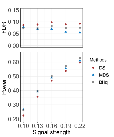
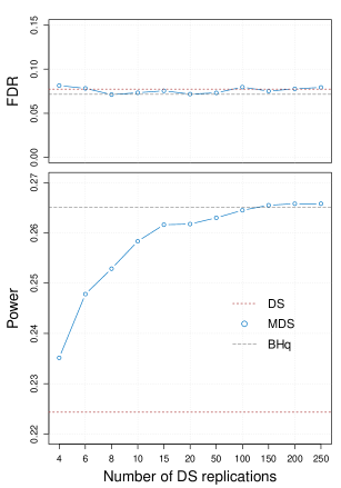
Refer to caption
Refer to caption
Figure 12: Empirical FDRs and powers for the Normal means model. Throughout, we set n=500๐‘›500n=500, p=800๐‘800p=800, and p1=160subscript๐‘1160p_{1}=160. For jโˆˆS1๐‘—subscript๐‘†1j\in S_{1}, the ฮผjsubscript๐œ‡๐‘—\mu_{j}โ€™s are independent samples from Nโ€‹(0,ฮด2)๐‘0superscript๐›ฟ2N(0,\delta^{2}). In the left panels, we fix the number of DS replications in MDS at m=200๐‘š200m=200 and vary the signal strength ฮด๐›ฟ\delta. In the right panels, we fix the signal strength at ฮด=0.08๐›ฟ0.08\delta=0.08 and vary the number of DS replications m๐‘šm. The designated FDR control level is q=0.1๐‘ž0.1q=0.1. Each dot in the figure represents the average from 50 independent runs.
Refer to caption
Refer to caption
Figure 13: ROC curves for the Normal means model. The x๐‘ฅx-axis and the y๐‘ฆy-axis denote the false positive rate (FPR) and the true positive rate (TPR), respectively. Throughout, we set n=500๐‘›500n=500, p=800๐‘800p=800, and p1=160subscript๐‘1160p_{1}=160. For jโˆˆS1๐‘—subscript๐‘†1j\in S_{1}, the ฮผjsubscript๐œ‡๐‘—\mu_{j}โ€™s are set to be ยฑฮดplus-or-minus๐›ฟ\pm\delta with random signs. ฮด=0.08๐›ฟ0.08\delta=0.08 and 0.160.160.16 in the left and the right panel, respectively. We set the number of DS replications in MDS at m=1000๐‘š1000m=1000. The designated FDR control level is q=0.5๐‘ž0.5q=0.5. Each dot in the figure represents the average from 50 independent runs.

6.3 Simulation details

To complement Section 4.1, we first detail the blockwise diagonal Toeplitz covariance matrix, of which each block along the diagonal is set to be

[1(pโ€ฒโˆ’2)โ€‹ฯpโ€ฒโˆ’1(pโ€ฒโˆ’3)โ€‹ฯpโ€ฒโˆ’1โ€ฆฯpโ€ฒโˆ’10(pโ€ฒโˆ’2)โ€‹ฯpโ€ฒโˆ’11(pโ€ฒโˆ’2)โ€‹ฯpโ€ฒโˆ’1โ€ฆ2โ€‹ฯpโ€ฒโˆ’1ฯpโ€ฒโˆ’1โ‹ฎโ‹ฑโ‹ฎ0ฯpโ€ฒโˆ’12โ€‹ฯpโ€ฒโˆ’1โ€ฆ(pโ€ฒโˆ’2)โ€‹ฯpโ€ฒโˆ’11],matrix1superscript๐‘โ€ฒ2๐œŒsuperscript๐‘โ€ฒ1superscript๐‘โ€ฒ3๐œŒsuperscript๐‘โ€ฒ1โ€ฆ๐œŒsuperscript๐‘โ€ฒ10missing-subexpressionmissing-subexpressionmissing-subexpressionmissing-subexpressionmissing-subexpressionmissing-subexpressionsuperscript๐‘โ€ฒ2๐œŒsuperscript๐‘โ€ฒ11superscript๐‘โ€ฒ2๐œŒsuperscript๐‘โ€ฒ1โ€ฆ2๐œŒsuperscript๐‘โ€ฒ1๐œŒsuperscript๐‘โ€ฒ1โ‹ฎmissing-subexpressionโ‹ฑmissing-subexpressionmissing-subexpressionโ‹ฎ0๐œŒsuperscript๐‘โ€ฒ12๐œŒsuperscript๐‘โ€ฒ1โ€ฆsuperscript๐‘โ€ฒ2๐œŒsuperscript๐‘โ€ฒ11\begin{bmatrix}1&\frac{(p^{\prime}-2)\rho}{p^{\prime}-1}&\frac{(p^{\prime}-3)\rho}{p^{\prime}-1}&\ldots&\frac{\rho}{p^{\prime}-1}&0\\ &&&&&\\ \vspace{0.5cm}\frac{(p^{\prime}-2)\rho}{p^{\prime}-1}&1&\frac{(p^{\prime}-2)\rho}{p^{\prime}-1}&\ldots&\frac{2\rho}{p^{\prime}-1}&\frac{\rho}{p^{\prime}-1}\\ \vspace{0.5cm}\vdots&&\ddots&&&\vdots\\ 0&\frac{\rho}{p^{\prime}-1}&\frac{2\rho}{p^{\prime}-1}&\ldots&\frac{(p^{\prime}-2)\rho}{p^{\prime}-1}&1\end{bmatrix}, (24)

where pโ€ฒ=p/10superscript๐‘โ€ฒ๐‘10p^{\prime}=p/10. Throughout, we refer ฯโˆˆ(0,1)๐œŒ01\rho\in(0,1) as the correlation factor.
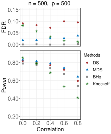
Refer to caption
Refer to caption
Figure 14: Empirical FDRs and powers of MDS using three different mirror statistics constructed with f1,f2,f3subscript๐‘“1subscript๐‘“2subscript๐‘“3f_{1},f_{2},f_{3} specified in (2). The algorithmic settings are as per Figure 3.
Refer to caption
Refer to caption
Figure 15: Empirical FDRs and powers for low-dimensional linear models. Features are independently drawn from Nโ€‹(0,ฮฃ)๐‘0ฮฃN(0,\Sigma) with ฮฃฮฃ\Sigma being a Toeplitz covariance matrix. Knockoff refers to the fixed-design knockoff filter (Barber and Candรจs, 2015). In the left panel, we fix the signal strength at ฮด=3๐›ฟ3\delta=3 and vary the correlation ฯ๐œŒ\rho. In the right panels, we fix the correlation at ฯ=0.6๐œŒ0.6\rho=0.6 and vary the signal strength ฮด๐›ฟ\delta. The designated FDR control level is q=0.1๐‘ž0.1q=0.1, and the number of relevant features is 50 across all settings. Each dot in the figure represents the average from 50 independent runs.
Refer to caption
Refer to caption
Figure 16: Standard deviations of the FDP for low-dimensional linear models with a Toeplitz correlation structure. The algorithmic settings are as per Figure 15.
Refer to caption
Refer to caption
Figure 17: Empirical FDRs and powers for linear models. The algorithmic settings are as per Figure 5.
Refer to caption
Refer to caption
Refer to caption
Refer to caption
Figure 18: Standard deviations of the FDP for linear models with a Toeplitz correlation structure. The algorithmic settings are as per Figure 5.
Refer to caption
Refer to caption
Refer to caption
Refer to caption
Figure 19: Empirical FDRs and powers for linear models. Features are independently drawn from Nโ€‹(0,ฮฃ)๐‘0ฮฃN(0,\Sigma) with ฮฃiโ€‹j=ฯ๐Ÿ™โ€‹(iโ‰ j)subscriptฮฃ๐‘–๐‘—superscript๐œŒ1๐‘–๐‘—\Sigma_{ij}=\rho^{\mathbbm{1}(i\neq j)}. In the left two panels, we fix the signal strength at ฮด=8๐›ฟ8\delta=8 and vary the pairwise correlation ฯ๐œŒ\rho. In the right two panels, we fix the pairwise correlation at ฯ=0.5๐œŒ0.5\rho=0.5 and vary the signal strength ฮด๐›ฟ\delta. The number of relevant features is 50 across all settings, and the designated FDR control level is q=0.1๐‘ž0.1q=0.1. Each dot in the figure represents the average from 50 independent runs.
Refer to caption
Refer to caption
Refer to caption
Refer to caption
Figure 20: Standard deviations of the FDP for linear models with a constant correlation structure. The algorithmic settings are as per Figure 19.
Refer to caption
Refer to caption
Figure 21: Standard deviations of the FDP for linear models with non-normal design matrices. The algorithmic settings are as per Figure 6.
Refer to caption
Refer to caption
Figure 22: Standard deviations of the FDP for linear models with a GWAS design matrix. The algoritmic settings are as per Figure 7.