Machine Learning Exchange-Correlation Potential in Time Dependent Density Functional Theory

Abstract

We propose a machine learning based approach to develop the exchange-correlation potential of time dependent density functional theory (TDDFT). The neural network projection from the time-varying electron densities to the corresponding correlation potentials in the time-dependent Kohn-Sham equation is trained using a few exact datasets for a model system of electron-hydrogen scattering. We demonstrate that this neural network potential can capture the complex structures in the time-dependent correlation potential during the scattering process and provide correct scattering dynamics, which are not obtained by the standard adiabatic functionals. We also show that it is possible to incorporate the nonadiabatic (or memory) effect in the potential with this machine learning technique, which significantly improves the accuracy of the dynamics. The method developed here offers a novel way to improve the exchange-correlation potential of TDDFT, which makes the theory a more powerful tool to study various excited state phenomena.

Time-dependent density functional theory (TDDFT) Runge and Gross (1984); Ullrich (2012); Maitra (2016) is a widely used first-principles approach to study the excited state properties of atoms, molecules and solids. TDDFT enables the first-principles simulation of correlated many-electron dynamics, which is in principle described by the time-dependent Schrödinger equation (TDSE) for the interacting system, by mapping it to the dynamics of the noninteracting [also called Kohn-Sham (KS)] system evolving in a single-particle potential. There have been many successful applications of TDDFT simulation to the interpretation and prediction of various excited state phenomena, e.g., the linear response and spectra of molecules and solids Botti et al. (2007); Adamo and Jacquemin (2013); Casida and Huix-Rotllant (2012); Byun and Ullrich (2017); Suzuki and Watanabe (2020), and real-time electron dynamics in systems exposed to external fields Wopperer et al. (2015); Chen et al. (2019); Yamada and Yabana (2019); Hübener et al. (2018); Dauth et al. (2016); Umerbekova et al. (2018) and in various non-equilibrium situations Kurth et al. (2010); Ueda et al. (2018); Curchod et al. (2013); Kurth and Stefanucci (2017); Pellegrini et al. (2015); Suzuki et al. (2018).

TDDFT is a formally exact theory, i.e., it ensures that the TDSE for the noninteracting (KS) system,

$$\begin{split}i\frac{\partial}{\partial t}&\Phi_{\rm KS}({\underline{\underline{\bf r}}},t)=(\sum_{i=1}^{N}[-\frac{\nabla^{2}_{i}}{2}+v_{\rm ext}({\bf r}_{i},t)\\ &+v_{\rm H}[n]({\bf r}_{i},t)+v_{\rm XC}[n,\Psi_{0},\Phi_{0}]({\bf r}_{i},t)])\Phi_{\rm KS}({\underline{\underline{\bf r}}},t),\end{split}$$ (1)

can, in theory, yield any observables of an $N$-electron system exactly and solely from the time-dependent electron density $n({\bf r},t)=N\int d^{N-1}{\bf r}|\Phi_{\rm KS}({\underline{\underline{\bf r}}},t)|^{2}$. (Throughout this paper, atomic units are used unless stated otherwise, and ${\underline{\underline{\bf r}}}\equiv\{{\bf r}_{1},{\bf r}_{2},\cdots,{\bf r}_{N}\}$.) Here, $v_{\rm ext}({\bf r},t)$ and $v_{\rm H}({\bf r},t)$ are the external potential applied to the system and the Hartree potential ($v_{\rm H}({\bf r},t)=\int d{\bf r^{\prime}}\frac{n({\bf r^{\prime}},t)}{|{\bf r}-{\bf r^{\prime}}|}$), respectively, and $v_{\rm XC}({\bf r},t)$ is the time-dependent (TD) exchange-correlation (XC) potential, which incorporates all many-body effects in the theory. The unique existence of the TDXC potential is proved by the Runge-Gross Runge and Gross (1984) and van Leeuwen van Leeuwen (1999) theorems; however, its exact form is unknown. It is known that the exact TDXC potential $v_{\rm XC}[n,\Psi_{0},\Phi_{0}]({\bf r},t)$ at time $t$, in principle, is functionally dependent on the history of the density $n({\bf r},t^{\prime}<t)$, the initial interacting many-body state $\Psi_{0}$, and the choice of the initial KS state $\Phi_{0}$, which indicates its exact form should be extremely complicated.

Therefore, almost all TDDFT applications to date use an adiabatic approximation, which inputs the instantaneous density into one of the existing XC potential functionals in the ground-state density functional theory (DFT) Koch and Holthausen (2001), and completely neglects both the history and initial-state dependence, i.e., lacks the memory effect Ullrich (2012); Maitra et al. (2002). It is true that the TDDFT calculation with these adiabatic functionals has achieved significant success in many studies Rozzi et al. (2013); E. Penka Fowe and Bandrauk (2011); Yabana et al. (2012); Castro et al. (2012); Miyamoto et al. (2015); Wang et al. (2015); Elliott et al. (2016); Schleife et al. (2015); Quashie et al. (2017). However, it has also been reported that there are many situations where these approximate TDXC potentials fail to even qualitatively reproduce the true dynamics Raghunathan and Nest (2012); Habenicht et al. (2014); Provorse and Isborn (2016); Wijewardane and Ullrich (2005). Recent studies on exactly-solvable model systems Elliott et al. (2012); Luo et al. (2014); Fuks et al. (2016); Thiele et al. (2008); Ramsden and Godby (2012); Elliott and Maitra (2012); Suzuki et al. (2017); Lacombe et al. (2018); Dittmann et al. (2018) have extensively explored the conditions where the adiabatic functional fails. One important finding is that, when the local acceleration of electron densities occurs, the correlation part ($v_{\rm C}$) of the exact TDXC potential $v_{\rm XC}$ ($=v_{\rm X}+v_{\rm C}$), exhibits complex dynamical structures Elliott et al. (2012); Suzuki et al. (2017) that arise from the memory effect and play significant roles to provide the correct dynamics. The electron scattering process is a typical situation where these complex structures in the TD correlation (TDC) potential appear, and it was revealed that the standard adiabatic functionals lack these structures Suzuki et al. (2017); Lacombe et al. (2018).

In this study, we propose a novel approach to improve the XC potential of TDDFT using a machine learning technique. Development of the XC functional in DFT by a machine learning based approach has been actively conducted recently Snyder et al. (2012); Brockherde et al. (2017); Li et al. (2016); Nagai et al. (2018); Hollingsworth et al. (2018); Schmidt et al. (2019); Nagai et al. (2019), which demonstrates it is a promising direction to improve the DFT. In particular, neural-network (NN) projection from the electron density to the ground-state XC potential was developed in a recent study Nagai et al. (2018), and it was demonstrated that the KS equation equipped with this NN functional provides accurate ground-state density and total energy for a one-dimensional two-electron model system, and has a remarkable transferability. In TDDFT, the TDXC potential functional can also be regarded as a projection $n\rightarrow v_{\rm XC}$, but here $n$ is the history of the density ($n({\bf r},t^{\prime}<t)$). Thus, the projection should be more complicated than that in DFT, which means that there is more expectation on a machine learning based approach to find such a complicated projection.

Here we construct the NN projection from the TD density $n({\bf r},t)$ to the TDC potential $v_{\rm C}({\bf r},t)$ for a model system of electron-hydrogen (e-H) scattering Suzuki et al. (2017); Lacombe et al. (2018), as one example where the existing approximate functionals fail to reproduce the complex structures in $v_{\rm C}({\bf r},t)$. We demonstrate that this NN TDC potential $v_{\rm TDC}^{\rm NN}$ captures the complex structures that appeared in the exact potential very well, and provide significantly improved time-resolved scattering dynamics compared to those obtained by the standard approximate functionals.

The e-H scattering model system studied in this work is the same as that used in the previous studies Suzuki et al. (2017); Lacombe et al. (2018). It is a one-dimensional two-electron system with the Hamiltonian: ${\hat{H}}(x_{1},x_{2})=\sum_{i=1,2}\left(-\frac{1}{2}\frac{\partial^{2}}{\partial x_{i}^{2}}+v_{\rm ext}(x_{i})\right)+W_{ee}(x_{1},x_{2})$, where $W_{ee}(x_{1},x_{2})=\frac{1}{\sqrt{(x_{1}-x_{2})^{2}+1}}$ is the soft-Coulomb interaction Javanainen et al. (1988); Villeneuve et al. (1996); Bandrauk and Shon (2002); Lein et al. (2000); Lein and Kümmel (2005); Tempel et al. (2009); Wagner et al. (2012) and the external potential $v_{\rm ext}(x)=-\frac{1}{\sqrt{(x+10)^{2}+1}}$ is the soft-Coulomb model of a H atom located at $x=-10.0$ a.u. The spatial part of the initial interacting wavefunction is $\Psi_{0}(x_{1},x_{2})=\frac{1}{\sqrt{2}}\left(\phi_{\rm H}(x_{1})\phi_{\rm WP}(x_{2})+\phi_{\rm WP}(x_{1})\phi_{\rm H}(x_{2})\right)$, where a singlet state is chosen for the spin part. $\phi_{\rm H}(x)$ is the ground-state of one electron alone in the external potential $v_{\rm ext}(x)$ and $\phi_{\rm WP}(x)=\left(2\alpha/\pi\right)^{\frac{1}{4}}e^{\left[-\alpha(x-x_{0})^{2}+ip(x-x_{0})\right]}$ is an incident Gaussian wavepacket ($\alpha=0.1$), which represent an electron initially localized at $x_{0}=10.0$ a.u. approaching the H atom with a certain momentum $p$. For this system, the full TDSE $i\partial_{t}\Psi(x_{1},x_{2},t)={\hat{H}}(x_{1},x_{2})\Psi(x_{1},x_{2},t)$ can be numerically solved exactly, and the resulting TD density (for the case of incident momentum $p=-1.5$ a.u. for our first example), which were already reported in Ref. Suzuki et al. (2017), are plotted as the red lines in the upper panel for different time slices in Fig. 1.

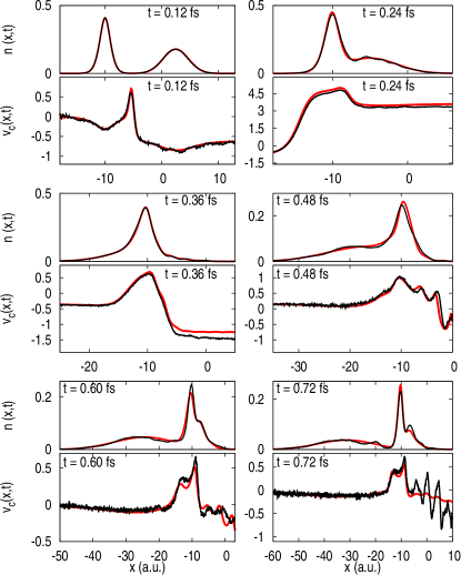
Figure 1: Snapshots of the trained NN TDC potential $v_{\rm TDC}^{\rm NN}$ for the initial KS state $\Phi_{0}^{(1)}$ in the e-H scattering model system (black line in the lower panel for each time slice) and the corresponding TD electron densities (black line in the upper panel) obtained by propagating the TDKS equation equipped with $v_{\rm TDC}^{\rm NN}$. Exact electron density (red line in the upper panel) and the exact TDC potential $v_{\rm TDC}^{\rm exact}$ (red line in the lower panel) are also plotted for each time slice.

As reported previously  Suzuki et al. (2017), for this case of $p=-1.5$ a.u., the scattering is inelastic, and some part of the wavepacket is reflected back after the collision at around 0.24 fs.

For this two-electron dynamics, the exact TDXC potential can be numerically obtained for any choice of the valid initial KS state that satisfies the van Leeuwen theorem Fuks et al. (2016); Elliott and Maitra (2012). Here, we focus on one natural choice for the initial KS state, i.e., the Slater determinant Suzuki et al. (2017); Elliott and Maitra (2012): $\Phi_{0}^{(1)}(x_{1},x_{2})=\phi_{0}(x_{1})\phi_{0}(x_{2})$ with one doubly-occupied spatial orbital $\phi_{0}(x)=\sqrt{\frac{n_{0}(x)}{2}}\exp\left[i\int^{x}\frac{j_{0}(x^{\prime})}{n_{0}(x^{\prime})}dx^{\prime}\right]$, where $n_{0}$ and $j_{0}$ are respectively the initial density and current density of the interacting system. For this initial KS state $\Phi_{0}^{(1)}$, the exact $v_{\rm X}(x,t)$ and $v_{\rm C}(x,t)$ can be numerically calculated Ullrich (2012); Elliott et al. (2012); Ruggenthaler et al. (2015); Nielsen et al. (2013) using the exact TD density $n(x,t)$ and current density $j(x,t)$ obtained from the solution of the TDSE. The numerically obtained $v^{\rm exact}_{\rm C}(x,t)$ (shown as the red lines in the lower panels of Fig. 1) exhibit complex peak- and valley-like structures that are crucial for scattering Suzuki et al. (2017).

In this study, we aim to make the NN learn this exact TD correlation potential $v^{\rm exact}_{\rm C}(x,t)$ because the exact functional form of $v^{\rm exact}_{\rm X}(x,t)$ ($=-\frac{1}{2}\int dx^{\prime}W_{ee}(x^{\prime},x)n(x^{\prime},t)$) is already known for the system under focus Ullrich (2012); Elliott et al. (2012). The structure of the NN TDC potential $v_{\rm TDC}^{\rm NN}$ constructed here is expressed as:

$$\begin{split}{\bf v}^{\rm NN}_{\rm TDC}=\cdots f[W^{(2)}f[W^{(1)}{\bf n}+{\bf b}^{(1)}]+{\bf b}^{(2)}]\cdots,\end{split}$$ (2)

where ${\bf v}^{\rm NN}_{\rm TDC}$ and n are the vectorized representations of $v_{\rm TDC}^{\rm NN}$ and $n$ ($f$ is a non-linear activation function (ReLU function Glorot et al. (2011) here), and $W^{(l)}$ ($l=1,2,\cdots$) and ${\bf b}^{(l)}$ are the weight matrices and bias vectors, of which the components are optimized to minimize the training error). As with the study on the NN XC potential in DFT Nagai et al. (2018), the form of Eq. (2) is, in principle, sufficiently flexible to be a numerically exact TDXC potential. The input vector ${\bf n}$ should ideally represent the entire history of the density ($n({\bf r},t^{\prime}<t)$); however, in the first example, the instantaneous density $n({\bf r},t)$ is used as ${\bf n}$.

The training procedure of the first example is as follows. First, the learning data set (${\bf n}^{(i)}(t_{j})$, ${\bf v}^{(i)}_{\rm TDC}(t_{j})$) is generated from the numerical calculation of $n(x,t)$ and $v^{\rm exact}_{\rm C}(x,t)$. Here, $i$ is the index that corresponds to the different scattering dynamics calculation with a different initial incident momentum, $p$. In the first example, five different initial momenta; $p=-1.0$, $-1.2$, $-1.4$, $-1.6$, $-1.8$ were employed to generate the training data set (thus $i=1,\cdots,5$). For each calculation with different $p$, the TDSE was numerically propagated with the discrete time step $\Delta t=2.4\times 10^{-3}$ fs up to $t=0.72$ fs, which corresponds to 300 time steps, and thus $j=1,\cdots,300$. Therefore, the $5\times 300=1500$ data set of (${\bf n}^{(i)}(t_{j})$, ${\bf v}^{(i)}_{\rm TDC}(t_{j})$) was generated. ${\bf n}^{(i)}(t_{j})$ and ${\bf v}^{(i)}_{\rm TDC}(t_{j})$ are the vectors obtained by the real-space discretization of $n^{(i)}(x,t_{j})$ and $v^{(i)}_{\rm TDC}(x,t_{j})$, respectively, onto common $N_{r}=1200$ uniform mesh points, i.e., ${\bf n}^{(i)}(t_{j})=\{n^{(i)}(x_{1},t_{j}),n^{(i)}(x_{2},t_{j}),\cdots,n^{(i)}(x_{N_{r}},t_{j})\}$ and ${\bf v}^{(i)}_{\rm TDC}(t_{j})=\{v^{(i)}_{\rm TDC}(x_{1},t_{j}),v^{(i)}_{\rm TDC}(x_{2},t_{j}),\cdots,v^{(i)}_{\rm TDC}(x_{N_{r}},t_{j})\}$.

The parameters of the NN (Eq. (2)) are then optimized with the generated data set using a similar method to that reported in Ref. Nagai et al. (2018): The fully connected NN with two hidden layers with 1200 nodes are used, and the root mean squared error between ${\bf v}^{(i)}_{\rm TDC}(t_{j})$ and those calculated from ${\bf n}^{(i)}(t_{j})$ by the NN is minimized with the adaptive moment estimation method (Adam) Kingma and Ba (2015) algorithm implemented in the Chainer package cha (2019). The initial estimate of the weight parameters is randomly generated and the optimization is stopped after 20000 epochs. Other details of the optimization are the same as those used in Ref. Nagai et al. (2018). This optimization procedure is sufficient to provide a NN that gives excellent results, as detailed later.

Finally, the trained NN TDC potential $v_{\rm TDC}^{\rm NN}$ is implemented in the time-dependent Kohn-Sham (TDKS) equation (Eq. (1)) for the initial KS state $\Phi_{0}^{(1)}$ with an initial incident momentum $p=-1.5$, which is out of the $p$ used for the training; that is, the test of the present NN is demonstrated by numerically integrating the TDKS equation for $\Phi_{0}^{(1)}$:

$$\begin{split}i\frac{\partial}{\partial t}&\phi(x,t)=[-\frac{\nabla^{2}}{2}+v_{\rm ext}(x,t)+v_{\rm H}[n](x,t)\\ &+v_{\rm X}[n](x,t)+v_{\rm TDC}^{\rm NN}(x,t)]\phi(x,t),\end{split}$$ (3)

over time, where $n(x,t)=2|\phi(x,t)|^{2}$ is calculated and the TDC potential is obtained from the NN ${\bf v}^{\rm NN}_{\rm TDC}$ on-the-fly at each time step, for the initial condition out of the training data set.

The resultant $n(x,t)$ and $v_{\rm TDC}^{\rm NN}(x,t)$ are plotted as black lines in the upper and lower panels of Fig. 1. It is evident that the black lines show similar structures to the exact ones (red lines); in particular, $v_{\rm TDC}^{\rm NN}$ captures the complex structures of the exact TDC potential, and the density dynamics reproduce the certain amount of reflection probability seen in the exact dynamics. Therefore, the machine learning based approach is confirmed as effective for the numerical implementation of $v_{\rm TDC}$, at least for this first example. From Fig. 1, $v_{\rm TDC}^{\rm NN}$ gradually exhibits spatially oscillating structures as times passes, which is due to the accumulation of small errors in the TD density, an intrinsic problem of the TD calculation that does not exist in the case of the NN potential for DFT. Nevertheless, the TD densities obtained from $v_{\rm TDC}^{\rm NN}$ show rather smooth structures during the entire simulation time (up to $t=0.72$ fs). This is achieved by the effect of the kinetic energy operator in Eq. (3) as a regulator of the artificial oscillation, as with that for the DFT case Nagai et al. (2018).

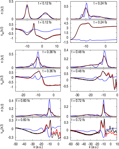
Figure 2: Snapshots of the NN TDXC potential with the memory effect $v_{\rm TDXC}^{\rm NNmemory}=v_{\rm X}+v_{\rm TDC}^{\rm NNmemory}$ for the same system shown in Fig. 1 (black line in the lower panel for each time slice) and the corresponding TD electron densities (black line in the upper panel). Exact (red lines) and ALDA (blue lines) results are also plotted for each time slice.

Now we consider a strategy for improvement of $v_{\rm TDC}^{\rm NN}$. Our first attempt to develop $v_{\rm TDC}^{\rm NN}$ does not take account of the memory effect of $n({\bf r},t^{\prime}<t)$ explicitly, i.e., the training data set was the combination of the instantaneous density $n(x,t)$ and $v^{\rm exact}_{\rm TDC}(x,t)$. Here we present how to incorporate the memory effect into $v_{\rm TDC}^{\rm NN}$. We assume that the density distribution immediately before $t$ has the most effect on $v_{\rm TDC}$ at $t$. Based on this hypothesis, we propose the following expression for the input vector n for the NN (Eq. (2)), so that it takes account of the memory effect:

$${\bf n}^{(i)}_{\{t_{0},t_{j}\}}=\{{\bf n}^{(i)}(t_{j}),{\bf N}^{(i)}(t_{j})\},$$ (4)

where ${\bf N}^{(i)}(t_{j})$ is the vector representation of

$$N^{(i)}(x,t_{j})=\int^{t_{j}}_{t_{0}}dt^{\prime}w\left(|t^{\prime}-t_{j}|\right)n(x,t^{\prime}),$$ (5)

and $w(t)$ is the weight function, for which we employed Gaussian function $w(t)=\frac{A}{\sqrt{2\pi\sigma^{2}}}\exp\left(-\frac{t^{2}}{2\sigma^{2}}\right)$. This additional input $N^{(i)}(x,t_{j})$ (Eq. (5)) in principle contains the history of $n$ from the initial time $t_{0}$, and $w(t)$ gives weight to the previous densities such that the more recent density has the larger effect. This idea can be regarded as a time version of the average density approximation (ADA) Gunnarsson et al. (1979) (The spatial version of ADA is a well-established technique to develop XC functional in DFT). ${\bf n}^{(i)}_{\{t_{0},t_{j}\}}$ is related to ${\bf v}^{(i)}_{\rm TDC}(t_{j})$ as one learning data set, i.e., the NN TDC potential trained with the memory effect, $v_{\rm TDC}^{\rm NNmemory}$, maps ${\bf n}_{\{t_{0},t_{j}\}}$ to ${\bf v}_{\rm TDC}(t_{j})$ at each time $t_{j}$.

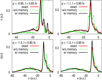
Figure 3: Snapshots of the electron density at $t=0.85$ fs obtained from different calculations: the exact TDSE calculation (red solid line), the TDKS equation equipped with the NN TDC potential without the memory effect (green dotted line), and with the memory effect (black solid line). The four panels correspond to the different initial incident momentum $p=-0.95$ (upper left), $-1.1$ (upper right), $-1.3$ (lower left) , and $-1.5$ (lower right).

We investigate the effectiveness of this method with $\sigma=2$ a.u. and $A=1$ . $v_{\rm TDC}^{\rm NNmemory}$ is trained using a similar procedure to that without the memory effect (The only difference is that the number of input nodes is now double, i.e., $1200\times 2=2400$. The number of hidden layer nodes is retained as $1200$). Figure 2 shows snapshots of the NN TDXC potential with memory, i.e., $v_{\rm TDXC}^{\rm NNmemory}=v_{\rm X}+v_{\rm TDC}^{\rm NNmemory}$ (black solid line in the lower panels) and the TD density (black solid lines in the upper panels) obtained through the solution of the TDKS equation with this NN potential. A comparison of these results with the exact results (red lines) reveals remarkable agreement between them, and the results obtained from the NN with memory shows better agreement than those obtained without memory (Fig. (1)); this is presented more clearly in Figs. 3 and 4 discussed later. We note that the exact TDXC potential (red line in the lower panels of Fig. (2)) and the exact TDC potential (red line in the lower panels of Fig. (1)) have almost the same structure, which indicates that the contribution of the TDX potential is small. It was previously reported that the dynamics calculated with only the exact TDX potential functional fail to reproduce the correct scattering Suzuki et al. (2017); Lacombe et al. (2018); therefore, it is essential to capture the features of the exact TDC potential correctly. In Fig. 2, the results obtained using the adiabatic local density approximation (ALDA) Entwistle et al. (2016); Casula et al. (2006); Helbig et al. (2011) to both the exchange and correlation potentials are also plotted as blue lines (same as those reported in Ref. Suzuki et al. (2017)). The ALDA XC potential, and other standard XC functionals (reported in Ref. Suzuki et al. (2017); Lacombe et al. (2018)), lack the important memory effect, and their structures are significantly different from the exact structure, which leads to a failure to yield the correct scattering. The NN TDC potential presented here, both with and without the memory effect, provides significantly better results than those from the standard functionals.

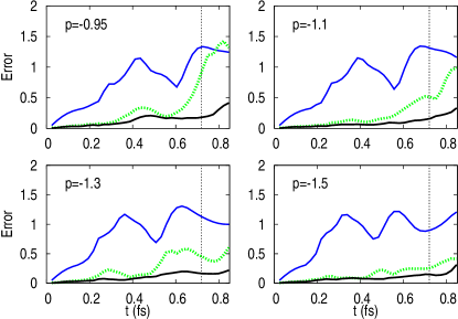
Figure 4: The error in the density for the NN TDC potential without the memory effect (green dotted line) and with the memory effect (black solid line), and ALDA (blue solid line) for the four different initial incident momenta; $p=-0.95$, $-1.1$, $-1.3$, and $-1.5$ (indicated inside each panel). Vertical dotted lines indicate the simulation time for the training dataset ($0.72$ fs).

To show the impact of incorporating the memory effect, and check the out-of-training transferability of the NN, we plot a comparison of the electron density at $t=0.85$ fs obtained from the different calculations in Fig. 3; the exact TDSE calculation (red solid line), the TDKS equation equipped with the NN TDC potential without the memory effect (green dotted line) and with the memory effect (black solid line) for the four different dynamics that start with different initial incident momenta; $p=-0.95$, $-1.1$, $-1.3$, and $-1.5$ (indicated inside each panel). None of these $p$ values are referenced in the training of the NN. In particular, $p=-0.95$ is outside the range of training dataset. Furthermore, the simulation time for these test dynamics (0.85 fs) is longer than that for the training dataset (0.72 fs). Therefore, the out-of-training transferability of the NN, both for the parameter of the system and the simulation time, can also be checked from Fig. 3. The results indicate that the NN potential with memory well reproduces the exact density at the time outside the training dataset for all $p$ cases. Remarkably, it even reproduces the exact density for $p=-0.95$, which is outside the range of $p$ used for the training. Thus, the out-of-training transferability of the NN potential with memory has been demonstrated. On the other hand, the density from the NN without memory has worse agreement with the exact density than that from the NN with memory, especially after $t=0.72$ fs and for $p=-0.95$ (this is also confirmed by Fig. 4 ; see below), which indicates a part of the memory effect is taken into account by the addition of $N^{(i)}(x,t_{j})$ into the input to the NN.

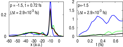
Figure 5: Snapshot of the electron density at $t=0.72$ fs for $p=-1.5$ obtained using $\Delta t=2.9\times 10^{-3}$ fs from the exact (red solid), NN TDC potential without the memory effect (green dotted) and with the memory effect (black solid) and ALDA (blue solid) calculations (left panel). Right panel shows the corresponding errors in the density.

To clearly reveal the superiority of the NN with memory over that without memory, the time evolution of the deviation of the TDKS density from the exact one, which is defined as $\int dx|n^{\rm exact}(x,t)-n^{\rm TDKS}(x,t)|$, is plotted for all $p$ in Fig. 4 (green dotted line: the NN TDC without memory, black solid line: the NN TDC with memory, and blue solid line: ALDA). This figure confirms the present findings: the NN TDC with memory gives better results than the NN TDC without memory. On the other hand, the ALDA gives poor results . Therefore, the validity of the proposed strategy to incorporate the memory effect by modification of the input density vector to Eq. (4) is demonstrated. We consider that the NN TDC potential with memory successfully captures not only the space nonlocality Koch and Holthausen (2001); Perdew et al. (2008), which is important to match the exact TDX potential, but also the time nonlocality (memory effect), at least for the model scattering problem investigated here.

We also point out the important advantage of the NN TDC potential using Eqs. (4) and (5) to take account of the memory effect; that is, this potential functional can be applied to simulations with different $\Delta t$ from that used in the training dataset, because the input $N^{(i)}(x,t_{j})$ is calculated by integrating the previous densities over time. Figure 5 shows the electron density at $t=0.72$ fs for $p=-1.5$ obtained from the calculations using $\Delta t=2.9\times 10^{-3}$ fs (left panel) and the corresponding errors in the density (right panel) (Note that the training dataset is obtained using $\Delta t=2.4\times 10^{-3}$ fs). Again, the NN TDC potential with memory exhibits the excellent results, showing its transferability to simulations with different size of time step.

We performed further test for the transferability of the NN with respect to the initial distance between the H atom and wavepacket and the parameter $\alpha$. The results (shown in the supplementary information (Fig. S1)) shows that the NN TDC potential has the transferability also with respect to these different parameters, although the number of training dataset needs to be increased. This indicates that expansion of the region where the NN TDC potential can be applied requires the expansion of the training data set. This situation is similar to that of the NN for the DFT, where the possible characteristic states need to be included in the training data set to make the NN have a wider transferability Nagai et al. (2018).

Further improvement of the NN is expected by enforcing the exact conditions of the TDXC potential, such as the zero force theorem Ullrich (2012), in the NN . The exact conditions are important because it ensure that the functional describes the correct physics, and recently it was employed to improve the NN functionals in DFT Hollingsworth et al. (2018). It could be possible to enforce the exact conditions in the NN for TDDFT as well, by using some specific functional form that satisfies the exact conditions regardless of the parameters optimized by the machine-leaning. This approach may also be used to suppress the oscillations in the NN potential. The use of the recurrent neural network (RNN)  Hopfield (1982) and long short term memory (LSTM) Hochreiter and Schmidhuber (1997) is also expected to show promise.

In summary, we have presented one example that indicates the novel approach based on the machine learning technique to develop the XC potential of TDDFT is effective. We have demonstrated that the NN TDC potential trained with a few numerically exact data sets reproduces the correct 1-dimensional two-electron scattering dynamics that are not included in the training data, which demonstrates its transferability. Furthermore, we have also shown that it is possible to incorporate the memory effect in this NN TDC potential, which significantly improves the result.

Our results indicate that once a few numerically exact (or sufficiently accurate) data of the many-body dynamics of interest are available, then it is possible to train the NN TDC (or TDXC) potential so that it can be used to simulate at least similar dynamics to those used in the training. Applications of the NN potential to other systems where the memory effect is known to crucial, such as the system in an electric field Elliott et al. (2012), is an important feature direction to investigate the need to further improve the functional form of NN to take account of the memory effect more effectively. The TDSE of an (three-dimensional) atom in a laser field can be numerically solved by means of the time-dependent variational principle method Rowan et al. (2020), and the resulting data can be used to train the NN TDXC potential, which can then be applied to the TDDFT calculation of actual molecules. It will also be possible to apply the machine learning approach to develop the XC kernel in linear-response TDDFT Botti et al. (2007); Adamo and Jacquemin (2013); Casida and Huix-Rotllant (2012); Byun and Ullrich (2017) using the many-body perturbation calculation results as training data. With these studies, TDDFT will become a more powerful tool for the study of various excited state phenomena.