Convex Fairness Constrained Model
Using Causal Effect Estimators
Abstract.
Recent years have seen much research on fairness in machine learning. Here, mean difference (MD) or demographic parity is one of the most popular measures of fairness. However, MD quantifies not only discrimination but also explanatory bias which is the difference of outcomes justified by explanatory features. In this paper, we devise novel models, called FairCEEs, which remove discrimination while keeping explanatory bias. The models are based on estimators of causal effect utilizing propensity score analysis. We prove that FairCEEs with the squared loss theoretically outperform a naive MD constraint model. We provide an efficient algorithm for solving FairCEEs in regression and binary classification tasks. In our experiment on synthetic and real-world data in these two tasks, FairCEEs outperformed an existing model that considers explanatory bias in specific cases.
1. Introduction
Recently much research on fairness in machine learning has been conducted. While numerous companies, scientific communities, and public organizations are collecting huge data repositories, the data tend to be biased toward an individual or a group based on their inherent or acquired characteristics, which are called sensitive features, such as race or gender. Machine learning models trained on such biased datasets may produce discriminatory predictions with respect to the sensitive feature. The problem of biased datasets is crucial to ensuring fairness when applying machine learning algorithms to applications such as loan assignment (Hardt et al., 2016), criminal risk assessment (Chouldechova, 2017), and school admissions (Friedler et al., 2016). It is necessary to develop fair decision-making methods that avoid discrimination arising from biased datasets.
Regarding fairness in machine learning, discrimination is considered either direct or indirect (Calders and Verwer, 2010). Direct discrimination is caused by a sensitive feature such as race or gender, while indirect discrimination is caused by non-sensitive features which are strongly correlated with the sensitive feature. Removing the sensitive feature from the input removes direct discrimination, but does not remove indirect discrimination. This is called the red lining effect (Calders and Verwer, 2010). Furthermore, as described in (Calders et al., 2013), the non-sensitive features that cause indirect discrimination sometimes include features which cause bias but can be justified. These features are called explanatory features and the bias caused by the explanatory features are called explanatory bias. We treat such explanatory bias as non-discriminatory by following the work of (Calders et al., 2013), though explanatory bias is included in indirect discrimination. Figure 1 shows the relationship between discrimination and explanatory bias.
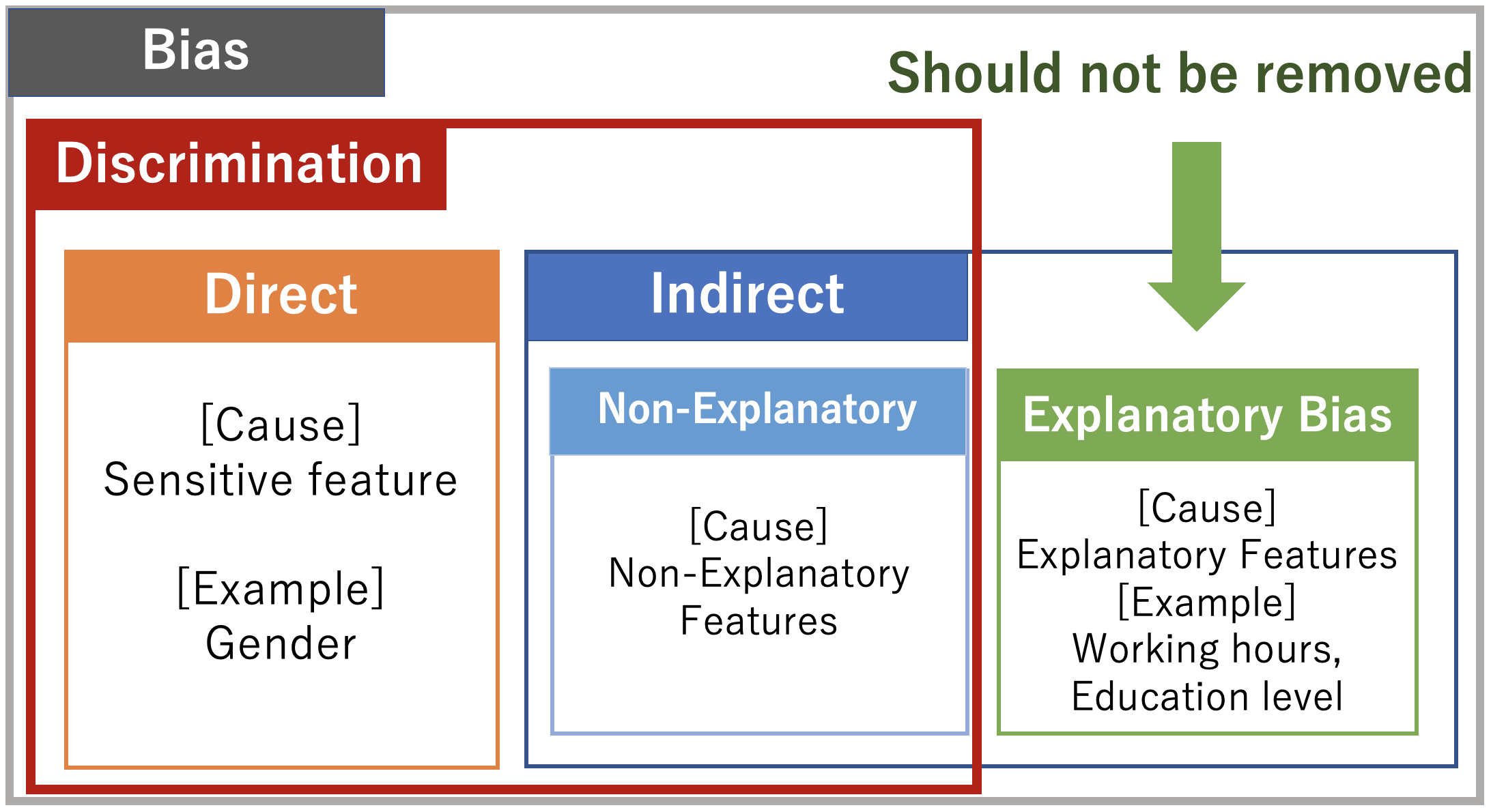
Researchers have introduced several statistical criteria (Hardt et al., 2016; Calders and Verwer, 2010; Zafar et al., 2017a; Dwork et al., 2012) in an attempt to formalize notions of fairness. Mean difference (MD) (Calders and Verwer, 2010) is one of the most popular measures of fairness to quantify discrimination. This measure is the difference of outcomes between groups distinguished by the sensitive feature. MD can quantify direct and indirect discrimination, but explanatory bias is also included in indirect discrimination. Therefore, when we use MD=0 as a constraint, we may mistakenly remove explanatory bias. This leads to reverse discrimination and degrades performance. Several studies based on MD (Calders and Verwer, 2010; Kamiran and Calders, 2009; Edwards and Storkey, 2015; Zafar et al., 2017b; Louizos et al., 2015) can suffer from this problem. In this paper, discrimination is defined as MD except for explanatory bias:
| (1) | Discrim. = MD - explanatory bias |
and use Discrim. =0 as a constraint in our model. Several studies have dealt with explanatory bias (Kamiran et al., 2013; Johnson et al., 2016; Kamiran and ŽliobaitÄ, 2013) from a non-causal perspective. In addition to them, there are mainly two research streams that have used estimators of causal effect (Rubin, 1974; Pearl, 2009) instead of MD. The recent work (Kusner et al., 2017; Kilbertus et al., 2017; Nabi and Shpitser, 2017; Zhang and Bareinboim, 2018b; Russell et al., 2017; Chiappa and Gillam, 2018; Zhang et al., 2018, 2017) uses causal diagrams for this purpose, but the resulting optimization problems tend to be difficult. Indeed, it seems difficult to find a global solution for such problems because of their non-convexity (Nabi and Shpitser, 2017; Zhang and Bareinboim, 2018a).
In this paper, we use propensity score analysis (Rosenbaum and Rubin, 1983) for simplifying the models used in other research. The papers (Qureshi et al., 2016; Calders et al., 2013) deal with explanatory bias based on propensity score analysis. In (Qureshi et al., 2016) the authors proposed a causal discrimination discovery approach using estimators of causal effect based on the propensity score. Although their work bears similarity to ours in terms of using estimators of causal effect, there are differences in that the estimator in (Qureshi et al., 2016) is calculated in its nearest neighbor such as in individual fairness (Dwork et al., 2012) and in that our model is for preventing discrimination, not for discovery. In (Calders et al., 2013) the authors proposed Multi MD, which removes discrimination and keeps explanatory bias on the basis of stratification (Rosenbaum and Rubin, 1984). However, unless the number of strata is set appropriately, the stratification may create a stratum that has some explanatory bias, which results in failure of Multi MD.
We propose new models, called Fair prediction using Causal Effect Estimators, (FairCEEs) that use another estimator based on the propensity score, the IPW (Rubin, 1985) or DR (Bang and Robins, 2005) estimator, for causal effect. Using the estimators for a constraint instead of MD makes it possible to remove the discrimination and keep the explanatory bias.
Our contributions are as follows:
-
•
FairCEEs based on the IPW and DR estimators of causal effect are formulated as simple convex quadratic optimizations; for classification, they are globally solved with the proximal gradient method; for regression, they are solved using the Lagrange multiplier method.
-
•
FairCEE-IPW and Multi MD theoretically outperform Single MD in regression tasks.
-
•
Numerical experiments on synthetic and real-world data show that FairCEEs outperform Multi MD in terms of fairness and prediction accuracy.
The organization of the paper is as follows: after preliminaries are introduced in Section 2, our model is described in Section 3. The algorithm and theoretical analysis are in Section 4. Section 5 describes numerical experiments on synthetic and real-world datasets. A conclusion follows.
2. Preliminaries
We review MD (Calders and Verwer, 2010), which is one of the most popular measures of fairness, and show an existing model Multi MD (Calders et al., 2013), which removes discrimination (1). Next, we point out the disadvantages of Multi MD. Finally, we describe the potential outcome model (Holland, 1986) and its relationship with Multi MD.
2.1. Notation
Suppose that and are the number of data and non-sensitive features, respectively and one sensitive feature exists in a given dataset. is a matrix consisting of non-sensitive feature values. indicates the feature values of the -th instance, i.e., the -th row of , and denotes the sensitive feature. is a binary variable such as male/female, denoted by . is the observed value of sensitive feature of the -th instance, and is the vector defined by . For convenience, we define two index sets and , defined by and . is the target label; in a regression task, , and in a binary classification task, , unless otherwise specified. is the observed label of the -th instance, and is the vector defined by . is the predicted label of the -th instance. In this paper, we consider a linear model class and denote the trainable parameter by , i.e, for regression or for classification where is a sigmoid function.
In what follows, we will consider the supervised learning setting, where we have a dataset (, , ) meaning (non-sensitive feature values, sensitive feature values, labels), and our goal is to train a model whose prediction does not include discrimination (1), but has good accuracy.
2.2. Single MD and Multi MD
MD is a measure quantifying how discriminatory the dataset is for classification and regression tasks.
Definition 2.1 (Mean Difference (Calders and Verwer, 2010)).
| (2) |
where is the size of the set . Note that by replacing with in the definition, MD represents how discriminatory the prediction is.
Now let us describe Single MD and Multi MD (Calders et al., 2013), which are related to our model. 111Single MD and Multi MD are denoted by SEM-S, SEM-MP in (Calders et al., 2013). Single MD is formulated as
| (3) |
where
| (4) |
From (2) and (4) and reminding that for and for , represents MD of outputs, and therefore, the constraint in (2.2) means MD=0. As mentioned in Section 1, Single MD does not consider explanatory bias; it is defined by (Calders et al., 2013) as the differences in outcomes of groups distinguished by a sensitive feature value that is explainable by explanatory features and can be justified. The explanatory features are denoted by , where is the number of explanatory features, while the non-explanatory feature values are denoted by . In our settings, the explanatory features are provided externally.
Remark 2.1.
It seems possible to remove non-explanatory discrimination without removing explanatory bias by using MD in an inequality constraint, i.e., with a hyperparameter , following (Komiyama et al., 2018; Zafar et al., 2017b; Agarwal et al., 2018) or in a regularizer, i.e., with a hyperparameter , as in (Kamishima et al., 2012; Berk et al., 2017; Zemel et al., 2013). However, these approaches require the correct explanatory bias in the hyperparameter , , but the true value of the explanatory bias is unknown. It is difficult to determine appropriate hyperparameter values because the criteria used in validation for hyperparameters is not clear. On the other hand, our approaches described later can remove discrimination while keeping explanatory bias without using hyperparameters.
Calders et al. (Calders et al., 2013) proposed Multi MD which utilizes stratification (Rosenbaum and Rubin, 1984) according to a propensity score (Rosenbaum and Rubin, 1983) for a constraint.
Definition 2.2 (Propensity Score (Rosenbaum and Rubin, 1983)).
Let and be the sensitive feature and the explanatory features, respectively. The propensity score is defined as
In general, because the true propensity score is unknown, we have to estimate it from the dataset. Usually this is done using a logistic regression model. Using this propensity score and stratification technique (Rosenbaum and Rubin, 1984), Multi MD can be formulated as follows (Calders et al., 2013). First, we estimate propensity scores. Then, we split the dataset into strata via the propensity score quantiles222Although is fixed to five in (Calders et al., 2013), we formulate the generalized form with various values of in this paper.. Next, we define Multi MD constraints as MD=0 in each stratum. Formally , , and are feature values, labels, sensitive feature values and constraint vector respectively, in the -th stratum.
| (5) |
where
In the same way as Single MD (2.2), represents the value of MD of outputs in the -th stratum.
2.3. Disadvantages of Multi MD
Multi MD removes Discrim. (1) by using stratification with respect to the propensity score. Here, we need an appropriately large number of strata , because if is too small, each stratum will have a range of propensity scores and some explanatory bias may remain in each stratum. Unfortunately, there are three cases where we can not increase the number of strata appropriately. In this paper, we refer these cases as Imbalance CASE, Degenerate CASE and Inferred CASE.
Imbalance CASE : the case where datasets are imbalanced with respect to the sensitive feature value of 0 or 1 (e.g. ). Here, splitting the dataset into many strata may create a stratum that has only a one-sided sensitive feature value. In that case, we can not calculate the MD, which leads to a failure of Multi MD. Since this case is likely to appear in fairness settings, it is a serious weakness of Multi MD.
Degenerate CASE : the case where the number of features is small. Here, setting leads to degeneration and the optimal solution of Multi MD (2.2) becomes the zero vector, which satisfies MD=0. This means that Multi MD with large removes explanatory bias incorrectly and degrades performance in this case.
Inferred CASE : the case where the estimated value of propensity score is close to . As well as Imbalance CASE, splitting the dataset into many strata may create a stratum that has only a one-sided sensitive feature value in this case.
2.4. Potential Outcome Model (POM)
Now let us describe the potential outcome model (POM) (Holland, 1986). Although the relationship between POM and Multi MD is not mentioned in (Calders et al., 2013), we should point out that the discrimination (1) referred to in (Calders et al., 2013) corresponds to the causal effect defined by POM. In Multi MD, the model estimates the causal effect by stratification (Rosenbaum and Rubin, 1984) and uses the estimated value for its constraint. Our model uses POM in a similar way.
POM considers potential outcome variables denoted by and . Target label has both the potential outcome that would have resulted if had received the sensitive feature , and the potential outcome that would have resulted if had received the sensitive feature . We can observe either of them, but not both. In other words, we can observe but not when is equal to 1. Formally, we can write . By using these variables, causal effect (Rubin, 1974) is defined as the difference between potential outcome variables.
| (6) |
Since we can observe either of them, but not both, estimating the causal effect is a missing data problem.
MD is generally not a consistent estimator of causal effect; i.e.,
because of covariates that are correlated with both and . If we regard the explanatory features as covariates, then the causal effect corresponds to Discrim. (1). This is the discrimination we want to remove. When we consider the discrimination as the causal effect (6), the true explanatory bias corresponds to
There are several methods of estimating causal effect by using a propensity score, including stratification (Rosenbaum and Rubin, 1984) used in (Calders et al., 2013). In this paper, instead of stratification, we use IPW and DR estimators, which are explained in Section 3.
3. Proposed Model
Now we propose new models, called Fair prediction using Causal Effect Estimators (FairCEEs). The estimators, IPW and DR, used for FairCEEs are defined below.
We can avoid the three CASEs described in Section 2.3 utilizing these estimators because they do not need dividing datasets into some strata. Although the sensitive feature is binary for simplicity, these models can be generalized to multiple groups.
3.1. FairCEE-IPW
Here, we introduce the Inverse Probability Weighting (IPW) estimator (Rubin, 1985) and give a formulation using it for its constraint. Note that we use the loss function as the objective function in the following formulations. We can apply our method to regression and binary classification tasks by setting to the squared loss () or logistic loss, respectively 333Note that the input of a sensitive feature is not used in the prediction models..
Definition 3.1 (IPW Estimator (Rubin, 1985)).
Here, is the propensity score for the -th instance. Accordingly, we define the IPW estimator of causal effect as
| (7) |
The IPW estimator is a consistent estimator of causal effect (6) under the assumption that the modeling for the propensity score is correct 444We can not confirm that the assumption holds because either of potential outcome variables is missing. However, in practice, we can check some metrics which measure the goodness of fit of the model such as AUC.. Accordingly, FairCEE-IPW is formulated as
| (8) |
where
| (9) |
3.2. FairCEE-DR
The other estimator of causal effect is the Doubly Robust (DR) estimator (Bang and Robins, 2005).
Definition 3.2 (DR Estimator (Bang and Robins, 2005)).
Here, is the propensity score of the -th instance. and are predictions of potential outcome variables () of the -th instance. Accordingly, we define DR estimator of causal effect as
In addition to modeling the propensity score, the DR estimator uses the modeling for and . Since either of the true values of and are unknown, we use the estimated values, i.e., and , instead of and . In this study, we train two models and for and , respectively. is trained using explanatory features whose index belongs to and is trained using explanatory features whose index is in . We use the output of and as and instead of and (i.e. and where is the explanatory feature values of the -th instance.)
We explained above that if the propensity score is incorrectly estimated, the IPW estimator will not be consistent. For this reason, the IPW estimator is not consistent in Inferred CASE. However, it is known that even if the estimated propensity score is wrong, the DR estimator remains a consistent estimator of causal effect as long as and are estimated correctly (see, e.g., (Bang and Robins, 2005)). We formulate FairCEE-DR as follows. (Note that and are defined in (9).)
| (10) |
where
As well as FairCEE-IPW, is the estimated value of DR estimator of the prediction (i.e. the constraint of (3.2) means DR=0.). Since the constraints of FairCEEs with a linear model are linear in terms of , we can solve them using algorithms described below555In general, the constraints of FairCEEs are linear with respect to outputs. Applying FairCEEs to a non-linear model may require another algorithm..
4. Algorithm and Analysis
In this section, we describe the algorithms for FairCEEs in regression and classification tasks. Then we show two theorems on the squared losses of FairCEE-IPW and Multi MD.
4.1. Algorithm for Regression and Classification
In a regression task, we use the squared loss function as . We can solve FairCEEs with the squared loss by using the Lagrange multiplier method as is done with Multi MD in (Calders et al., 2013).
In a binary classification task, we use the logistic loss function as in FairCEEs (3.1) and (3.2). Then we solve them with the proximal gradient method (PGM) (see, e.g., (Beck, 2017)). FairCEEs, Single MD and Multi MD can be formulated in the following generalized form666Note that our algorithm can be applied to not only FairCEEs but also Single MD and Multi MD for binary classification.. Let and be a constant matrix and vector, respectively, for constraints. is the number of constraints. In Multi MD, is equal to . In the other methods, is equal to 1. Let be the binary label for the -th instance.
| (11) |
Next, we apply the proximal gradient method to (4.1). Algorithm 4.1 is an overview of our algorithm777In our algorithm, we use a backtracking line search with a clipping process (), which prevents the step size from being less than ., where .
The following theorem implies that the proximal gradient method, Algorithm 4.1, has a convergence rate of . {algorithm} PGM for FairCEEs \lx@orig@algorithmic \REQUIRE \STATE \STATEInitialize \FOR \WHILETrue \STATE \STATE \IF \STATEKeep as \STATEBreak \ELSE\STATE \ENDIF\ENDWHILE\ENDFOR
Theorem 4.1.
Proof.
With the help of references such as (Nesterov, 2004), the statement can be proved if the gradient vector of is Lipschitz continuous with a constant (called -smooth); i.e., there exists a constant that satisfies
Next, we prove that the logistic loss function is -smooth function and .
First, we show that is an -smooth function. Since , and , we can say the inequality , which means that is an -smooth function with equal to 1.
Next, we consider the following logistic loss function.
We define . The derivative is by the chain rule.
Accordingly, we can obtain the following inequalities:
This means that the logistic loss is an -smooth function and .
∎
4.2. Theoretical Analysis
Now we show some theoretical guarantees for the proposed model, FairCEE-IPW (3.1). The following theorem says that our model FairCEE-IPW can achieve a smaller training error than Single MD (2.2) under a reasonable assumption. The assumption in the theorem is that the value estimated by the IPW estimator on a dataset (i.e. ) is less than the value estimated by MD (), and the assumption is likely to hold as discussed in the end of this section.
Theorem 4.2 (FairCEE-IPW Loss).
Lemma 4.1 (Loss of optimal solution).
Consider an optimization problem formulated as follows.
Let be the optimal solution of the above optimization problem. Then, the value of loss function is obtained as follows when is optimal (i.e )
Proof.
The optimal solution satisfies the constraint . Then, we have
We get
where is the angle between and .
Here, since is the optimal solution, we can say
∎
Lemma 4.2 (The norm of MD constraint vector).
Proof.
From the definition of , we can prove the lemma.
∎
Next, we prove Theorem 4.2.
Proof.
We can say
As with the previous theorem, we can show that Multi MD (2.2) also can achieve a smaller training error than Single MD (2.2).
Theorem 4.3 (Multi MD Loss).
Proof.
Let be the MD of the -th stratum (i.e. ).
Let be as follows.
We define , in the same way. By using this new notation and the original problem’s constraint, the optimal solution of the original problem satisfies this following equality.
The original problem can be rewritten as follows.
We get the following inequality:
where and are the index subsets of for the -th stratum.
Theorem 4.3 says that if the mean of MD in each stratum corresponding to is smaller than MD on the entire dataset, the optimal value of the squared loss in Multi MD (2.2) is less than that of Single MD (2.2).
When the dataset includes explanatory bias and the model of the propensity score is correct, by the definition of discrimination (1), the causal effect estimated by the IPW estimator and stratification are less than MD. Therefore, these assumptions of Theorem 4.2 and 4.3 are reasonable for our settings. From these two theorems, we can say both FairCEE-IPW and Multi MD give fair predictions and their losses are smaller than that of Single MD. We leave the analysis of FairCEE-DR to future work.
5. Numerical experiments
We obtained numerical results on synthetic data and real-world data in an attempt to answer the following research questions.
-
•
(RQ1) Do the three CASEs mentioned in Section 2.3 degrade the performance of Multi MD?
-
•
(RQ2) Do FairCEEs work in the three CASEs?
-
•
(RQ3) Do FairCEEs work on real-world data?
Since we know the true explanatory bias in the synthetic data (it is unknown in the real-world data), it is easy to understand the results. Hence, we first analyzed the behavior of FairCEEs and Multi MD in detail in an experiment using synthetic data. After that, we experimented using three real-world data in regression and binary classification tasks.
5.1. Dataset and Experimental Setup
5.1.1. Synthetic Data
Here we explain how to generate synthetic dataset for the regression task. We focus on only the synthetic dataset for the regression because it is not easy to generate a dataset for classification whose explanatory bias is known. We generated of instances with . The rest of the dataset had instances with . If the instance had a positive sensitive feature (i.e. ), we drew the explanatory feature values and non-explanatory feature values from the following different multivariate normal distributions.
In the same way, if the instance had a negative sensitive feature (i.e. ), we drew samples from the following distributions.
where and is an identity matrix. After sampling and , we generate the label of the -th instance as follows.
where are explanatory feature values, non-explanatory feature values and noise of the -th instance respectively ().
In this synthetic data, we can know the discrimination (6) and the true explanatory bias.
Since we know the values of these parameters used to generate the synthetic data, we can calculate Discrim. and the explanatory bias.
In our experiments, we created the three CASEs of Section 2.3 by modifying the parameters of the synthetic data. Unless otherwise specified, we generated the synthetic data with , , , and . We set when generating Imbalance CASE and and when generating Degenerate CASE. In Inferred CASE, we set and (in other case, by default).
5.1.2. Real-world Data
| datasets | |||||
|---|---|---|---|---|---|
| C&C | 1994 | 99 | race | (970, 1024) | Crime Rate |
| COMPAS | 5855 | 14 | race | (2914, 2941) | Recidivism |
| ADULT | 30162 | 101 | gender | (20380, 9782) | Income |
We used three real-world datasets. We conducted experiments on two tasks, regression and binary classification. In the regression task, we used C&C888https://archive.ics.uci.edu/ml/datasets/communities+and+crime. In the binary classification task, we used COMPAS (Angwin and Kirchner, 2016) and ADULT999https://archive.ics.uci.edu/ml/datasets/adult. Table 1 shows the statistics of these real-world data after the preprocessing.
The ADULT101010The ADULT dataset is a weighted dataset. So this is not a good real-world dataset as typically used. However, we use it to verify the performance of FairCEEs since much research use this dataset (Zafar et al., 2017b; Agarwal et al., 2019; Pleiss et al., 2017; Lipton et al., 2018; Donini et al., 2018). and C&C datasets are in the UCI repository (Dua and Graff, 2017). We followed (Komiyama et al., 2018) when preprocessing the COMPAS datasets and followed (Calders et al., 2013) when preprocessing the C&C dataset. When we preprocessed the ADULT dataset, we removed missing data and binarized its categorical features and normalized its continuous features. We chose the explanatory features by following (Calders et al., 2013) for C&C and by following (Qureshi et al., 2016) for ADULT. In the COMPAS dataset, we determined the explanatory features by conducting a dependency analysis following (Calders et al., 2013), whereby features that are highly correlated to both the target and the sensitive feature represent potential covariates.
5.1.3. Experimental Setup
We used FairCEE-IPW (3.1) and FairCEE-DR (3.2) (respectively referred to as fcee_ipw and fcee_dr in the figures below). For comparison, we compared FairCEEs to methods using propensity score analysis111111The methods using causal diagrams also deal with the explanatory bias. However, it is difficult to compare it fairly because the performance of methods using causal diagrams depends on the causal diagrams we assume. . We used the Multi MD (2.2) and Single MD (2.2) models for comparison, The figures below refer to Multi MD with strata as multi_ and Single MD as single. The sensitive feature was not used in the prediction models. We conducted the experiments on the synthetic data 50 times and added error bars to the results. We ran our script once on each real-world dataset because solving classification problem by FariCEEs and Multi MD took more time than regression task.
5.2. Disadvantages of Multi MD (RQ1)
|
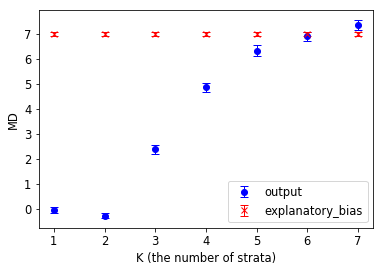
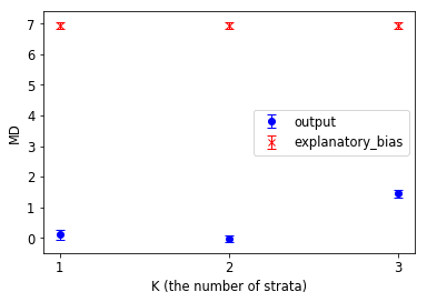
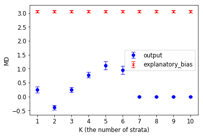
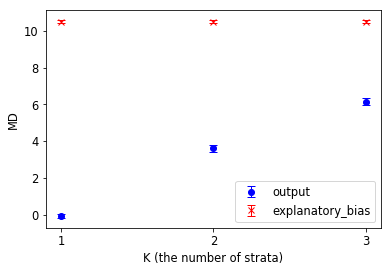
Now let us discuss the results of our experiment investigating the performance of Multi MD in the three CASEs described in Section 2.3. First, we show that Multi MD with a small incorrectly removes explanatory bias. Next, we show that it is difficult to set a large enough in the three CASEs.
In Figures 2 and 3, by the definition of Discrim. (1), it is desirable that the MD of Multi MD is close to the explanatory bias (i.e. Discrim. is close to 0). Figure 2 shows that the MD of Multi MD with few strata is much less than the explanatory bias. This is because when is too small, each stratum has a range of propensity scores and some explanatory bias may remain in each stratum.
Figure 3 indicated that it is impossible to split the dataset into more than three strata because of imbalances with respect to the sensitive feature. Figure 3 shows that MDs of Multi MD with are all zero. This is because degeneration causes the optimal solution of Multi MD to become the zero vector. When the number of strata is less than seven, the MD of the outputs is much less than the explanatory bias. This represents reverse discrimination because of few strata. As well as Figure 3, Figure 3 shows that it is impossible to split the dataset into more than three strata because the estimated values of propensity scores are nearly equal to the sensitive features. Figures 3, 3 and 3 show that in the three CASEs, Multi MD can not increase appropriately and Multi MD mistakenly removes the explanatory bias.
5.3. Comparison between FairCEEs and Multi MD in the three CASEs (RQ2)
|
| Single MD | Multi MD | IPW | DR | |
|---|---|---|---|---|
| Imbalance CASE | 48.614 | 10.262 | 6.808 | 6.538 |
| Degenerate CASE | 9.418 | 0.793 | 0.221 | 0.217 |
| Inferred CASE | 110.459 | 14.870 | 21.361 | 1.603 |
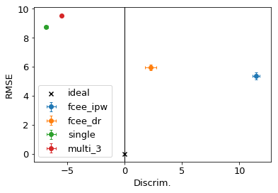
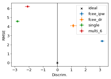
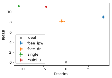
Next we show that FairCEEs outperform Multi MD in terms of loss and fairness in the three CASEs. Figure 4 is the loss-bias tradeoff graph in the three CASEs. The vertical axis represents RMSE, while the horizontal axis represents Discrim. (1). Note that, as mentioned in Section 5.1, we know the explanatory bias only in the experiment on synthetic data. Our goal here is to train a model that is fair at the expense of a small increase in loss. Accordingly, the loss and Discrim. should be close to 0 in Figure 4 (this corresponds to the ideal point). Figure 4 is the result of the comparison between FairCEEs and Multi MD in the three CASEs. Since it was found in Section 5.2 that cannot be more than three in Imbalance CASE and Inferred CASE or more than seven in Degenerate CASE, we compare FairCEEs with Multi MD with in Imbalance CASE and Inferred CASE and in Degenerate CASE. Figure 4 shows that the RMSE and Discrim. of FairCEE-DR are closer to 0 than those of Multi MD in the three CASEs. These results show that our FairCEE-DR outperforms Multi MD in terms of loss and fairness in the three CASEs.
In addition, we calculated the squared error between each estimated value for Discrim. (1) and the true value of Discrim. in the three CASEs to investigate how precisely the IPW and DR estimators estimate Discrim. (1). The result is in Table 2. This table indicates that the squared error between the IPW or DR estimator and Discrim.121212Note that SE of Multi MD is defined as , where is the MD of the -th stratum. is much smaller than that of MD or Stratification used in Single or Multi MD in Imbalance CASE and Degenerate CASE. It also shows the DR estimator is the most accurate in all the CASEs including Inferred CASE. This is because the model for the propensity score is wrong and the IPW estimator can not accurately estimate Discrim., whereas the DR estimator works appropriately because of the robustness due to the estimators for and .
|
5.4. Evaluation in Real-world Data (RQ3)
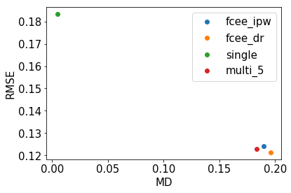
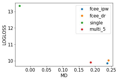
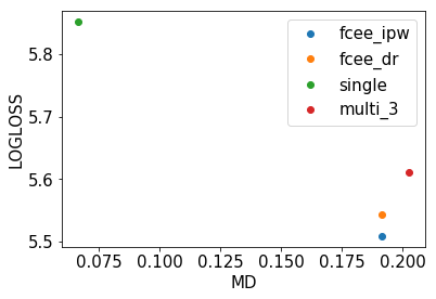
We visualized the results for the real-world data in the form of a loss-bias tradeoff graph as in Section 5.3. Note that we can not calculate Discrim. because we do not know the explanatory bias in the experiment on the real-world data. Thus, MD is the horizontal axis instead of Discrim. Here, because MD includes explanatory bias, it is not desirable that MD equal 0. Thus, we can not plot the ideal point, unlike in Figure 4. We used the logistic loss instead of RMSE in a binary classification task.
Figures 5 and 5 show that the MDs of the FairCEEs are larger than that of Multi MD, but the losses of FairCEE-DR and FairCEE-IPW are smaller than those of Multi MD in Figure 5 and 5, respectively. It is difficult to say which is superior, as we do not know the true explanatory bias. Figure 5 shows that the loss and MD of FairCEE-IPW are larger than those of Multi MD. This is probably because the model for the propensity score is not so good and the IPW estimator can not estimate the causal effect precisely. On the other hand, FairCEE-DR appropriately removes discrimination. This is because DR estimator can robustly estimate the causal effect by utilizing the estimators for and .
The ADULT dataset in Figure 5 is imbalanced with respect to the sensitive feature (see Table 1). Therefore, for the same reason as in Imbalance CASE, we can not increase appropriately. Actually, Multi MD did not work when we set . Therefore, we used Multi MD with three strata on the ADULT dataset. Figure 5 shows that the loss and MD of FairCEEs are lower than those of Multi MD. This indicates that FairCEEs outperform Multi MD in terms of loss and fairness in the ADULT dataset, which belongs to Imbalance CASE. This result is consistent with the results of the experiment on synthetic data in Section 5.3.
6. Conclusion and Future Work
We described FairCEEs based on IPW and DR estimators of causal effect that can remove discrimination while keeping explanatory bias. The proximal gradient method is applicable to FairCEEs with the logistic loss. We showed that FairCEE-IPW and Multi MD theoretically outperform Single MD in regression tasks. Our experiment on synthetic and real-world data indicated that FairCEE-DR outperforms Multi MD in cases where Multi MD does not work well due to too few strata.
By including a linear constraint of IPW=0 or DR=0, existing machine learning models can take into account reasonable fairness that eliminates explanatory bias. In this paper we only focused on regression and classification machine learning models, but this constraint can be used in a general framework. We would like to guarantee the validity of the general machine learning fairness model for future work. We have considered the setting with one binary sensitive feature in this paper. It may be possible to generalize most results of the paper to the settings of multiple sensitive features or a sensitive feature with multiple levels, i.e. by considering causal effects in regard to each sensitive feature. We would like to investigate it further.
References
- (1)
- Agarwal et al. (2018) Alekh Agarwal, Alina Beygelzimer, Miroslav Dudik, John Langford, and Hanna Wallach. 2018. A Reductions Approach to Fair Classification. In Proceedings of the 35th International Conference on Machine Learning (Proceedings of Machine Learning Research), Jennifer Dy and Andreas Krause (Eds.), Vol. 80. PMLR, Stockholmsmässan, Stockholm Sweden, 60–69. http://proceedings.mlr.press/v80/agarwal18a.html
- Agarwal et al. (2019) Alekh Agarwal, Miroslav Dudik, and Zhiwei Steven Wu. 2019. Fair Regression: Quantitative Definitions and Reduction-Based Algorithms. In Proceedings of the 36th International Conference on Machine Learning (Proceedings of Machine Learning Research), Kamalika Chaudhuri and Ruslan Salakhutdinov (Eds.), Vol. 97. PMLR, Long Beach, California, USA, 120–129. http://proceedings.mlr.press/v97/agarwal19d.html
- Angwin and Kirchner (2016) Larson Jeff Mattu Surya Angwin, Julia and Lauren. Kirchner. 2016. Machine Bias: There’s software used across the country to predict future criminals. https://www.propublica.org/.
- Bang and Robins (2005) Heejung Bang and James M. Robins. 2005. Doubly robust estimation in missing data and causal inference models. Biometrics 61 (2005), 692–972.
- Beck (2017) Amir Beck. 2017. First-Order Methods in Optimization. SIAM-Society for Industrial and Applied Mathematics, Philadelphia.
- Berk et al. (2017) R. Berk, H. Heidari, S. Jabbari, M. Joseph, M. Kearns, J. Morgenstern, S. Neel, and A. Roth. 2017. A Convex Framework for Fair Regression. FAT-ML Workshop (2017).
- Calders et al. (2013) Toon Calders, Asim Karim, Faisal Kamiran, Wasif Ali, and Xiangliang Zhang. 2013. Controlling Attribute Effect in Linear Regression. 2013 IEEE 13th International Conference on Data Mining (2013), 71–80.
- Calders and Verwer (2010) Toon Calders and Sicco Verwer. 2010. Three naive Bayes approaches for discrimination-free classification. Data Mining and Knowledge Discovery 21, 2 (01 Sep 2010), 277–292. https://doi.org/10.1007/s10618-010-0190-x
- Chiappa and Gillam (2018) Silvia Chiappa and Thomas Gillam. 2018. Path-Specific Counterfactual Fairness. Proceedings of the AAAI Conference on Artificial Intelligence 33 (02 2018). https://doi.org/10.1609/aaai.v33i01.33017801
- Chouldechova (2017) Alexandra Chouldechova. 2017. Fair Prediction with Disparate Impact: A Study of Bias in Recidivism Prediction Instruments. Big Data 5, 2 (2017), 153–163. https://doi.org/10.1089/big.2016.0047 arXiv:https://doi.org/10.1089/big.2016.0047 PMID: 28632438.
- Donini et al. (2018) Michele Donini, Luca Oneto, Shai Ben-David, John S Shawe-Taylor, and Massimiliano Pontil. 2018. Empirical Risk Minimization Under Fairness Constraints. In Advances in Neural Information Processing Systems 31, S. Bengio, H. Wallach, H. Larochelle, K. Grauman, N. Cesa-Bianchi, and R. Garnett (Eds.). Curran Associates, Inc., 2791–2801. http://papers.nips.cc/paper/7544-empirical-risk-minimization-under-fairness-constraints.pdf
- Dua and Graff (2017) Dheeru Dua and Casey Graff. 2017. UCI Machine Learning Repository. http://archive.ics.uci.edu/ml
- Dwork et al. (2012) Cynthia Dwork, Moritz Hardt, Toniann Pitassi, Omer Reingold, and Richard Zemel. 2012. Fairness Through Awareness (ITCS ’12). ACM, New York, NY, USA, 214–226. https://doi.org/10.1145/2090236.2090255
- Edwards and Storkey (2015) Harrison A Edwards and Amos J. Storkey. 2015. Censoring Representations with an Adversary. CoRR abs/1511.05897 (2015).
- Friedler et al. (2016) Sorelle A. Friedler, Carlos Scheidegger, and Suresh Venkatasubramanian. 2016. On the (im)possibility of fairness. arXiv e-prints, Article arXiv:1609.07236 (Sep 2016), arXiv:1609.07236 pages. arXiv:cs.CY/1609.07236
- Hardt et al. (2016) Moritz Hardt, Eric Price, and Nathan Srebro. 2016. Equality of Opportunity in Supervised Learning (NIPS’16). Curran Associates Inc., USA, 3323–3331. http://dl.acm.org/citation.cfm?id=3157382.3157469
- Holland (1986) Paul W. Holland. 1986. Statistics and Causal Inference. J. Amer. Statist. Assoc. 81, 396 (1986), 945–960. http://www.jstor.org/stable/2289064
- Johnson et al. (2016) Kory D. Johnson, Dean P. Foster, and Robert A. Stine. 2016. Impartial Predictive Modeling: Ensuring Fairness in Arbitrary Models. arXiv e-prints, Article arXiv:1608.00528 (Aug 2016), arXiv:1608.00528 pages. arXiv:stat.ME/1608.00528
- Kamiran and ŽliobaitÄ (2013) Faisal Kamiran and IndrÄ Å½liobaitÄ. 2013. Explainable and Non-explainable Discrimination in Classification. In Discrimination and Privacy in the Information Society.
- Kamiran and Calders (2009) F. Kamiran and T. Calders. 2009. Classifying without discriminating. In 2009 2nd International Conference on Computer, Control and Communication. 1–6. https://doi.org/10.1109/IC4.2009.4909197
- Kamiran et al. (2013) Faysal Kamiran, Indre Zliobaite, and Toon Calders. 2013. Quantifying explainable discrimination and removing illegal discrimination in automated decision making. Knowledge and Information Systems 35, 3 (2013), 613–644. https://doi.org/10.1007/s10115-012-0584-8
- Kamishima et al. (2012) Toshihiro Kamishima, Shotaro Akaho, Hideki Asoh, and Jun Sakuma. 2012. Fairness-Aware Classifier with Prejudice Remover Regularizer. In Machine Learning and Knowledge Discovery in Databases, Peter A. Flach, Tijl De Bie, and Nello Cristianini (Eds.). Springer Berlin Heidelberg, Berlin, Heidelberg, 35–50.
- Kilbertus et al. (2017) Niki Kilbertus, Mateo Rojas-Carulla, Giambattista Parascandolo, Moritz Hardt, Dominik Janzing, and Bernhard Schölkopf. 2017. Avoiding Discrimination Through Causal Reasoning (NIPS’17). Curran Associates Inc., USA, 656–666. http://dl.acm.org/citation.cfm?id=3294771.3294834
- Komiyama et al. (2018) Junpei Komiyama, Akiko Takeda, Junya Honda, and Hajime Shimao. 2018. Nonconvex Optimization for Regression with Fairness Constraints. In Proceedings of the 35th International Conference on Machine Learning (Proceedings of Machine Learning Research), Jennifer Dy and Andreas Krause (Eds.), Vol. 80. PMLR, Stockholmsmässan, Stockholm Sweden, 2737–2746. http://proceedings.mlr.press/v80/komiyama18a.html
- Kusner et al. (2017) Matt J Kusner, Joshua Loftus, Chris Russell, and Ricardo Silva. 2017. Counterfactual Fairness. In Advances in Neural Information Processing Systems 30, I. Guyon, U. V. Luxburg, S. Bengio, H. Wallach, R. Fergus, S. Vishwanathan, and R. Garnett (Eds.). Curran Associates, Inc., 4066–4076. http://papers.nips.cc/paper/6995-counterfactual-fairness.pdf
- Lipton et al. (2018) Zachary Lipton, Julian McAuley, and Alexandra Chouldechova. 2018. Does mitigating ML's impact disparity require treatment disparity? In Advances in Neural Information Processing Systems 31, S. Bengio, H. Wallach, H. Larochelle, K. Grauman, N. Cesa-Bianchi, and R. Garnett (Eds.). Curran Associates, Inc., 8125–8135. http://papers.nips.cc/paper/8035-does-mitigating-mls-impact-disparity-require-treatment-disparity.pdf
- Louizos et al. (2015) Christos Louizos, Kevin Swersky, Yujia Li, Max Welling, and Richard S. Zemel. 2015. The Variational Fair Autoencoder. CoRR abs/1511.00830 (2015).
- Nabi and Shpitser (2017) Razieh Nabi and Ilya Shpitser. 2017. Fair Inference On Outcomes. Proceedings of AAAI Conference on Artificial Intelligence 2018 (05 2017).
- Nesterov (2004) Yurii Nesterov. 2004. Introductory Lectures on Convex Optimization. Springer US, New York.
- Pearl (2009) Judea Pearl. 2009. Causality: Models, Reasoning and Inference (2nd ed.). Cambridge University Press, New York, NY, USA.
- Pleiss et al. (2017) Geoff Pleiss, Manish Raghavan, Felix Wu, Jon Kleinberg, and Kilian Q. Weinberger. 2017. On Fairness and Calibration (NIPS’17). Curran Associates Inc., USA, 5684–5693. http://dl.acm.org/citation.cfm?id=3295222.3295319
- Qureshi et al. (2016) Bilal Qureshi, Faisal Kamiran, Asim Karim, and Salvatore Ruggieri. 2016. Causal Discrimination Discovery Through Propensity Score Analysis. arXiv e-prints, Article arXiv:1608.03735 (Aug 2016), arXiv:1608.03735 pages. arXiv:cs.CY/1608.03735
- Rosenbaum and Rubin (1983) Paul R. Rosenbaum and Donald B. Rubin. 1983. The central role of the propensity score in observational studies for causal effects. Biometrika 70, 1 (04 1983), 41–55. https://doi.org/10.1093/biomet/70.1.41 arXiv:http://oup.prod.sis.lan/biomet/article-pdf/70/1/41/662954/70-1-41.pdf
- Rosenbaum and Rubin (1984) Paul R. Rosenbaum and Donald B. Rubin. 1984. Reducing Bias in Observational Studies Using Subclassification on the Propensity Score. J. Amer. Statist. Assoc. 79, 387 (1984), 516–524. https://doi.org/10.1080/01621459.1984.10478078 arXiv:https://amstat.tandfonline.com/doi/pdf/10.1080/01621459.1984.10478078
- Rubin (1974) Donald B. Rubin. 1974. Estimating causal effects of treatments in randomized and nonrandomized studies. Journal of Educational Psychology 66 (10 1974), 688–701. https://doi.org/10.1037/h0037350
- Rubin (1985) Donald. B. Rubin. 1985. The Use of Propensity Scores in Applied Bayesian Inference. In Bayesian Statistics 2. North-Holland/Elsevier (Amsterdam; New York), 463–472.
- Russell et al. (2017) Chris Russell, Matt J Kusner, Joshua Loftus, and Ricardo Silva. 2017. When Worlds Collide: Integrating Different Counterfactual Assumptions in Fairness. In Advances in Neural Information Processing Systems 30, I. Guyon, U. V. Luxburg, S. Bengio, H. Wallach, R. Fergus, S. Vishwanathan, and R. Garnett (Eds.). Curran Associates, Inc., 6414–6423. http://papers.nips.cc/paper/7220-when-worlds-collide-integrating-different-counterfactual-assumptions-in-fairness.pdf
- Zafar et al. (2017a) Muhammad Bilal Zafar, Isabel Valera, Manuel Gomez Rodriguez, and Krishna P. Gummadi. 2017a. Fairness Beyond Disparate Treatment & Disparate Impact: Learning Classification without Disparate Mistreatment (WWW ’17). 1171–1180. https://doi.org/10.1145/3038912.3052660
- Zafar et al. (2017b) Muhammad Bilal Zafar, Isabel Valera, Manuel Gomez-Rodriguez, and Krishna P. Gummadi. 2017b. Fairness Constraints: Mechanisms for Fair Classification. In Proceedings of the 20th International Conference on Artificial Intelligence and Statistics, AISTATS 2017, 20-22 April 2017, Fort Lauderdale, FL, USA. 962–970. http://proceedings.mlr.press/v54/zafar17a.html
- Zemel et al. (2013) Rich Zemel, Yu Wu, Kevin Swersky, Toni Pitassi, and Cynthia Dwork. 2013. Learning Fair Representations. In Proceedings of the 30th International Conference on Machine Learning (Proceedings of Machine Learning Research), Sanjoy Dasgupta and David McAllester (Eds.), Vol. 28. PMLR, Atlanta, Georgia, USA, 325–333. http://proceedings.mlr.press/v28/zemel13.html
- Zhang and Bareinboim (2018a) Junzhe Zhang and Elias Bareinboim. 2018a. Equality of Opportunity in Classification: A Causal Approach. In Advances in Neural Information Processing Systems 31, S. Bengio, H. Wallach, H. Larochelle, K. Grauman, N. Cesa-Bianchi, and R. Garnett (Eds.). Curran Associates, Inc., 3671–3681. http://papers.nips.cc/paper/7625-equality-of-opportunity-in-classification-a-causal-approach.pdf
- Zhang and Bareinboim (2018b) Junzhe Zhang and Elias Bareinboim. 2018b. Fairness in Decision-Making ― The Causal Explanation Formula. In Proceedings of AAAI Conference on Artificial Intelligence. 2037–2045. https://www.aaai.org/ocs/index.php/AAAI/AAAI18/paper/view/16949
- Zhang et al. (2017) Lu Zhang, Yongkai Wu, and Xintao Wu. 2017. A Causal Framework for Discovering and Removing Direct and Indirect Discrimination. In Proceedings of the Twenty-Sixth International Joint Conference on Artificial Intelligence, IJCAI-17. 3929–3935. https://doi.org/10.24963/ijcai.2017/549
- Zhang et al. (2018) L. Zhang, Y. Wu, and X. Wu. 2018. Causal Modeling-Based Discrimination Discovery and Removal: Criteria, Bounds, and Algorithms. IEEE Transactions on Knowledge and Data Engineering (2018), 1–1. https://doi.org/10.1109/TKDE.2018.2872988