11institutetext: University of Haifa, Computer Science Department, Israel 11email: muradtuk@gmail.com, dannyf.post@gmail.com 22institutetext: MIT CSAIL, Cambridge, USA 22email: {baykal, rus}@mit.edu

On Coresets for Support Vector Machinesthanks: This research was supported in part by the U.S. National Science Foundation (NSF) under Awards 1723943 and 1526815, Office of Naval Research (ONR) Grant N00014-18-1-2830, Microsoft, and JP Morgan Chase.

Murad Tukan These authors contributed equally to this work.11    Cenk Baykal 22    Dan Feldman 11    Daniela Rus 22
Abstract

We present an efficient coreset construction algorithm for large-scale Support Vector Machine (SVM) training in Big Data and streaming applications. A coreset is a small, representative subset of the original data points such that a models trained on the coreset are provably competitive with those trained on the original data set. Since the size of the coreset is generally much smaller than the original set, our preprocess-then-train scheme has potential to lead to significant speedups when training SVM models. We prove lower and upper bounds on the size of the coreset required to obtain small data summaries for the SVM problem. As a corollary, we show that our algorithm can be used to extend the applicability of any off-the-shelf SVM solver to streaming, distributed, and dynamic data settings. We evaluate the performance of our algorithm on real-world and synthetic data sets. Our experimental results reaffirm the favorable theoretical properties of our algorithm and demonstrate its practical effectiveness in accelerating SVM training.

1 Introduction

Popular machine learning algorithms are computationally expensive, or worse yet, intractable to train on massive data sets, where the input data set is so large that it may not be possible to process all the data at one time. A natural approach to achieve scalability when faced with Big Data is to first conduct a preprocessing step to summarize the input data points by a significantly smaller, representative set. Off-the-shelf training algorithms can then be run efficiently on this compressed set of data points. The premise of this two-step learning procedure is that the model trained on the compressed set will be provably competitive with the model trained on the original set – as long as the data summary, i.e., the coreset, can be generated efficiently and is sufficiently representative.

Coresets are small weighted subsets of the training points such that models trained on the coreset are approximately as good as the ones trained on the original (massive) data set. Coreset constructions were originally introduced in the context of computational geometry [1] and subsequently generalized for applications to other problems, such as logistic regression, neural network compression, and mixture model training [6, 7, 11, 18, 21] (see [10] for a survey).

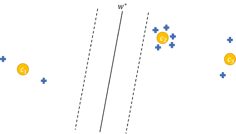
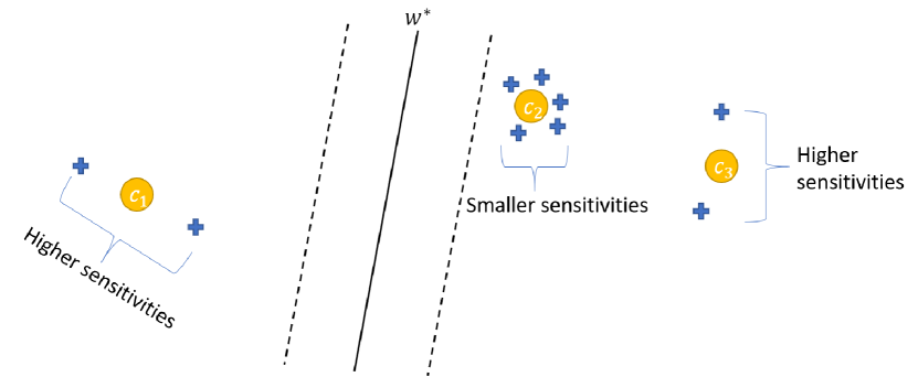
A popular coreset construction technique – and the one that we leverage in this paper – is to use importance sampling with respect to the points’ sensitivities. The sensitivity of each point is defined to be the worst-case relative impact of each data point on the objective function. Points with high sensitivities have a large impact on the objective value and are sampled with correspondingly high probability, and vice-versa. The main challenge in generating small-sized coresets often lies in evaluating the importance of each point in an accurate and computationally-efficient way.

1.1 Our Contributions

In this paper, we propose an efficient coreset construction algorithm to generate compact representations of large data sets to accelerate SVM training. Our approach hinges on bridging the SVM problem with that of k𝑘k-means clustering. As a corollary to our theoretical analysis, we obtain theoretical justification for the widely reported empirical success of using k𝑘k-means clustering as a way to generate data summaries for large-scale SVM training. In contrast to prior approaches, our approach is both (i) provably efficient and (ii) naturally extends to streaming or dynamic data settings. Above all, our approach can be used to enable the applicability of any off-the-shelf SVM solver – including gradient-based and/or approximate ones, e.g., Pegasos [27], to streaming and distributed data settings by exploiting the composibility and reducibility properties of coresets [10].

In particular, this paper contributes the following:

  1. 1.

    A coreset construction algorithm for accelerating SVM training based on an efficient importance sampling scheme.

  2. 2.

    An analysis proving lower bounds on the number of samples required by any coreset construction algorithm to approximate the input data set.

  3. 3.

    Theoretical guarantees on the efficiency and accuracy of our coreset construction algorithm.

  4. 4.

    Evaluations on synthetic and real-world data sets that demonstrate the effectiveness of our algorithm in both streaming and offline settings.

2 Related Work

Training SVMs requires 𝒪(n3)𝒪superscript𝑛3\mathcal{O}(n^{3}) time and 𝒪(n2)𝒪superscript𝑛2\mathcal{O}(n^{2}) space in the offline setting where n𝑛n is the number of training points. Towards the goal of accelerating SVM training in the offline setting, [28, 29] introduced the Core Vector Machine (CVM) and Ball Vector Machine (BVM) algorithms, which are based on reformulating the SVM problem as the Minimum Enclosing Ball (MEB) problem and Enclosing Ball (EB) problem, respectively, and by leveraging existing coreset constructions for each; see [5]. However, CVM’s accuracy and convergence properties have been noted to be at times inferior relative to those of existing SVM implementations [22]; moreover, unlike the algorithm presented in this paper, neither the CVM, nor the BVM algorithm extends naturally to streaming or dynamic settings where data points are continuously inserted or deleted. Similar geometric approaches, including extensions of the MEB formulation, those based on convex hulls and extreme points, among others, were investigated by [2, 12, 14, 16, 24, 26]. Another class of related work includes the use of canonical optimization algorithms such as the Frank-Wolfe algorithm [8], Gilbert’s algorithm [8, 9], and a primal-dual approach combined with Stochastic Gradient Descent (SGD) [15].

SGD-based approaches, such as Pegasos [27], have been a popular tool of choice in approximately-optimal SVM training. Pegasos is a stochastic sub-gradient algorithm for obtaining a (1+ε)1𝜀(1+\varepsilon)-approximate solution to the SVM problem in 𝒪~(dnλ/ε)~𝒪𝑑𝑛𝜆𝜀\widetilde{\mathcal{O}}(dn\lambda/\varepsilon) time for a linear kernel, where λ𝜆\lambda is the regularization parameter and d𝑑d is the dimensionality of the input data points. In contrast to our method, these approaches and their corresponding theoretical guarantees do not feasibly extend to dynamic data sets and/or streaming settings. In particular, gradient-based approaches cannot be trivially extended to streaming settings since the arrival of each input point in the stream results in a change of the gradient.

There has been prior work in streaming algorithms for SVMs, such as those of [2, 14, 25, 26]. However, these works generally suffer from poor practical performance in comparison to that of approximately optimal SVM algorithms in the offline (batch) setting, high difficulty of implementation and application to practical settings, and/or lack of strong theoretical guarantees. Unlike the algorithms of prior work, our method is simultaneously simple-to-implement, exhibits theoretical guarantees, and naturally extends to streaming and dynamic data settings, where the input data set is so large that it may not be possible to store or process all the data at one time.

3 Problem Definition

Let P={(x,y):xd×1,y{±1}}𝑃conditional-set𝑥𝑦formulae-sequence𝑥superscript𝑑1𝑦plus-or-minus1P=\left\{(x,y)\,:\,x\in\mathbb{R}^{d}\times{1},y\in\left\{\pm 1\right\}\right\} denote a set of n𝑛n input points. Note that for each point p=(x,y)P𝑝𝑥𝑦𝑃p=(x,y)\in P, the last entry xd+1=1subscript𝑥𝑑11x_{d+1}=1 of x𝑥x accounts for the bias term embedding into the feature space111We perform this embedding for ease of presentation later on in our analysis.. To present our results with full generality, we consider the setting where the input points P𝑃P may have weights associated with them. Hence, given P𝑃P and a weight function u:P0:𝑢𝑃subscriptabsent0u:P\to\mathbb{R}_{\geq 0}, we let 𝒫=(P,u)𝒫𝑃𝑢\mathcal{P}=(P,u) denote the weighted set with respect to P𝑃P and u𝑢u. The canonical unweighted case can be represented by the weight function that assigns a uniform weight of 1 to each point, i.e., u(p)=1𝑢𝑝1u(p)=1 for every point pP𝑝𝑃p\in P. For every TP𝑇𝑃T\subseteq P, let U(T)=pTu(p)𝑈𝑇subscript𝑝𝑇𝑢𝑝U{\left(T\right)}=\sum_{p\in T}u(p). We consider the scenario where n𝑛n is much larger than the dimension of the data points, i.e., ndmuch-greater-than𝑛𝑑n\gg d.

For a normal to a separating hyperplane wd+1𝑤superscript𝑑1w\in\mathbb{R}^{d+1}, let w1:dsubscript𝑤:1𝑑w_{1:d} denote vector which contains the first d𝑑d entries of w𝑤w. The last entry of w𝑤w (wd+1subscript𝑤𝑑1w_{d+1}) encodes the bias term b𝑏b\in\mathbb{R}. Under this setting, the hinge loss of any point p=(x,y)P𝑝𝑥𝑦𝑃p=(x,y)\in P with respect to a normal to a separating hyperplane, wd+1𝑤superscript𝑑1w\in\mathbb{R}^{d+1}, is defined as h(p,w)=[1yx,w]+𝑝𝑤subscriptdelimited-[]1𝑦𝑥𝑤h(p,w)=\left[1-y\langle x,w\rangle\right]_{+}, where []+=max{0,}subscriptdelimited-[]0\left[\cdot\right]_{+}=\max\{0,\cdot\}. As a prelude to our subsequent analysis of sensitivity-based sampling, we quantify the contribution of each point p=(x,y)P𝑝𝑥𝑦𝑃p=(x,y)\in P to the SVM objective function as

fλ(p,w)=12U(P)w1:d22+λh(p,w),subscript𝑓𝜆𝑝𝑤12𝑈𝑃superscriptsubscriptnormsubscript𝑤:1𝑑22𝜆𝑝𝑤f_{\lambda}(p,w)=\frac{1}{2U{\left(P\right)}}\left\|w_{1:d}\right\|_{2}^{2}+\lambda h(p,w), (1)

where λ[0,1]𝜆01\lambda\in[0,1] is the SVM regularization parameter, and h(p,w)=[1yx,w]+𝑝𝑤subscriptdelimited-[]1𝑦𝑥𝑤h(p,w)=\left[1-y\langle x,w\rangle\right]_{+} is the hinge loss with respect to the query wd+1𝑤superscript𝑑1w\in\mathbb{R}^{d+1} and point p=(x,y)𝑝𝑥𝑦p=(x,y). Putting it all together, we formalize the λ𝜆\lambda-regularized SVM problem as follows.

Definition 1 (λ𝜆\lambda-regularized SVM Problem)

For a given weighted set of points 𝒫=(P,u)𝒫𝑃𝑢\mathcal{P}=(P,u) and a regularization parameter λ[0,1]𝜆01\lambda\in[0,1], the λ𝜆\lambda-regularized SVM problem with respect to 𝒫𝒫\mathcal{P} is given by

minwd+1Fλ(𝒫,w),subscript𝑤superscript𝑑1subscript𝐹𝜆𝒫𝑤\min_{w\in\mathbb{R}^{d+1}}F_{\lambda}(\mathcal{P},w),

where

Fλ(𝒫,w)=p𝒫u(p)f(p,w).subscript𝐹𝜆𝒫𝑤subscript𝑝𝒫𝑢𝑝𝑓𝑝𝑤F_{\lambda}(\mathcal{P},w)=\sum\limits_{p\in\mathcal{P}}u(p)f(p,w). (2)

We let wsuperscript𝑤w^{*} denote the optimal solution to the SVM problem with respect to 𝒫𝒫\mathcal{P}, i.e., wargminwd+1Fλ(𝒫,w)superscript𝑤subscript𝑤superscript𝑑1subscript𝐹𝜆𝒫𝑤w^{*}\in\operatorname*{\arg\!\min}_{w\in\mathbb{R}^{d+1}}F_{\lambda}(\mathcal{P},w). A solution w^d+1^𝑤superscript𝑑1\hat{w}\in\mathbb{R}^{d+1} is an ξ𝜉\xi-approximation to the SVM problem if Fλ(𝒫,w^)Fλ(𝒫,w)+ξsubscript𝐹𝜆𝒫^𝑤subscript𝐹𝜆𝒫superscript𝑤𝜉F_{\lambda}(\mathcal{P},\hat{w})\leq F_{\lambda}(\mathcal{P},w^{*})+\xi. Next, we formalize the coreset guarantee that we will strive for when constructing our data summaries.

Coresets.

A coreset is a compact representation of the full data set that provably approximates the SVM cost function (2) for every query wd+1𝑤superscript𝑑1w\in\mathbb{R}^{d+1} – including that of the optimal solution wsuperscript𝑤w^{*}. We formalize this notion below for the SVM problem with objective function Fλ()subscript𝐹𝜆F_{\lambda}(\cdot) as in (2) below.

Definition 2 (ε𝜀\varepsilon-coreset)

Let ε(0,1)𝜀01\varepsilon\in(0,1) and let 𝒫=(P,u)𝒫𝑃𝑢\mathcal{P}=(P,u) be the weighted set of training points as before. A weighted subset SS=(S,v)SS𝑆𝑣\SS=(S,v), where SP𝑆𝑃S\subset P and v:S0:𝑣𝑆subscriptabsent0v:S\to\mathbb{R}_{\geq 0} is an ε𝜀\varepsilon-coreset for 𝒫𝒫\mathcal{P} if

wd+1|Fλ(𝒫,w)Fλ(SS,w)|εFλ(𝒫,w).formulae-sequencefor-all𝑤superscript𝑑1subscript𝐹𝜆𝒫𝑤subscript𝐹𝜆SS𝑤𝜀subscript𝐹𝜆𝒫𝑤\displaystyle\forall{w\in\mathbb{R}^{d+1}}\quad\left|F_{\lambda}\left(\mathcal{P},w\right)-F_{\lambda}\left(\SS,w\right)\right|\leq\varepsilon F_{\lambda}\left(\mathcal{P},w\right). (3)

This strong guarantee implies that the models trained on the coreset SSSS\SS with any off-the-shelf SVM solver will be approximately (and provably) as good as the optimal solution wsuperscript𝑤w^{*} obtained by training on the entire data set 𝒫𝒫\mathcal{P}. This also implies that, if the size of the coreset is provably small, e.g., logartihmic in n𝑛n (see Sec. 5), then an approximately optimal solution can be obtained much more quickly by training on SSSS\SS rather than 𝒫𝒫\mathcal{P}, leading to computational gains in practice for both offline and streaming data settings (see Sec. 6).

The difficulty in constructing coresets lies in constructing them (i) efficiently, so that the preprocess-then-train pipeline takes less time than training on the full data set and (ii) accurately, so that important data points – i.e., those that are imperative to obtaining accurate models – are not left out of the coreset, and redundant points are eliminated so that the coreset size is small. In the following sections, we introduce and analyze our coreset algorithm for the SVM problem.

4 Method

Our coreset construction scheme is based on the unified framework of [11, 18] and is shown in Alg. 1. The crux of our algorithm lies in generating the importance sampling distribution via efficiently computable upper bounds (proved in Sec. 5) on the importance of each point (Lines 11). Sufficiently many points are then sampled from this distribution and each point is given a weight that is inversely proportional to its sample probability (Lines 11). The number of points required to generate an ε𝜀\varepsilon-coreset with probability at least 1δ1𝛿1-\delta is a function of the desired accuracy ε𝜀\varepsilon, failure probability δ𝛿\delta, and complexity of the data set (t𝑡t from Theorem 5.3). Under mild assumptions on the problem at hand (see Sec. 0.A.4), the required sample size is polylogarithmic in n𝑛n.

Input : A set of training points Pd+1×{1,1}𝑃superscript𝑑111P\subseteq\mathbb{R}^{d+1}\times\{-1,1\} containing n𝑛n points, weight function u:P0:𝑢𝑃subscriptabsent0u:P\to\mathbb{R}_{\geq 0}, a regularization parameter λ[0,1]𝜆01\lambda\in[0,1], an approximation factor ξ>0𝜉0\xi>0, a positive integer k𝑘k, a sample size m𝑚m
Output : An weighted set (S,v)𝑆𝑣(S,v) which satisfies Theorem 5.3
1 w~~𝑤absent\tilde{w}\leftarrow An ξ𝜉\xi-approximation for the optimal SVM of (P,u)𝑃𝑢(P,u);
2 opt~ξFλ(𝒫,w~)ξsubscript~𝑜𝑝𝑡𝜉subscript𝐹𝜆𝒫~𝑤𝜉\widetilde{opt}_{\xi}\leftarrow F_{\lambda}(\mathcal{P},\tilde{w})-\xi;
3for y{,+}𝑦y\in\{-,+\} do
4       Pysubscript𝑃𝑦absentP_{y}\leftarrow all the points in P𝑃P that are associated with the label y𝑦y;
5       (cy(i),Py(i))i=1ksuperscriptsubscriptsuperscriptsubscript𝑐𝑦𝑖superscriptsubscript𝑃𝑦𝑖𝑖1𝑘absent\left(c_{y}^{(i)},P_{y}^{(i)}\right)_{i=1}^{k}\leftarrow k-means++(𝒫𝒫\mathcal{P}, k𝑘k);
6       for every i[k]𝑖delimited-[]𝑘i\in[k] do
7             αy(i)U(PPy(i))2λU(P)U(Py(i))superscriptsubscript𝛼𝑦𝑖𝑈𝑃superscriptsubscript𝑃𝑦𝑖2𝜆𝑈𝑃𝑈superscriptsubscript𝑃𝑦𝑖\alpha_{y}^{(i)}\leftarrow\frac{U{\left(P\setminus P_{y}^{(i)}\right)}}{2\lambda U{\left(P\right)}U{\left(P_{y}^{(i)}\right)}};
8             for every p=(x,y)Py(i)𝑝𝑥𝑦superscriptsubscript𝑃𝑦𝑖p=(x,y)\in P_{y}^{(i)} do
9                   pΔcy(i)yxsubscript𝑝Δsuperscriptsubscript𝑐𝑦𝑖𝑦𝑥p_{\Delta}\leftarrow c_{y}^{(i)}-yx;
10                   γ(p)u(p)U(Py(i))+λu(p)92max{49αy(i),4(αy(i))2+2pΔ229opt~ξ2αy(i)}𝛾𝑝𝑢𝑝𝑈superscriptsubscript𝑃𝑦𝑖𝜆𝑢𝑝9249superscriptsubscript𝛼𝑦𝑖4superscriptsuperscriptsubscript𝛼𝑦𝑖22superscriptsubscriptnormsubscript𝑝Δ229subscript~𝑜𝑝𝑡𝜉2superscriptsubscript𝛼𝑦𝑖\gamma(p)\leftarrow\frac{u(p)}{U{\left(P_{y}^{(i)}\right)}}+\lambda u(p)\frac{9}{2}\max\left\{\frac{4}{9}\alpha_{y}^{(i)},\sqrt{4\left(\alpha_{y}^{(i)}\right)^{2}+\frac{2\left\|p_{\Delta}\right\|_{2}^{2}}{9\widetilde{opt}_{\xi}}}-2\alpha_{y}^{(i)}\right\};
11            
12      
13
14tpPγ(p)𝑡subscript𝑝𝑃𝛾𝑝t\leftarrow\sum_{p\in P}\gamma(p);
15 (S,v)m𝑆𝑣𝑚(S,v)\leftarrow m weighted samples from 𝒫=(P,u)𝒫𝑃𝑢\mathcal{P}=(P,u) where each point pP𝑝𝑃p\in P is sampled with probability q(p)=γ(p)t𝑞𝑝𝛾𝑝𝑡q(p)=\frac{\gamma(p)}{t} and, if sampled, has weight v(p)=u(p)mq(p)𝑣𝑝𝑢𝑝𝑚𝑞𝑝v(p)=\frac{u(p)}{mq(p)};
16 return (S,v)𝑆𝑣(S,v);
Algorithm 1 Coreset(P,u,λ,ξ,k,m)Coreset𝑃𝑢𝜆𝜉𝑘𝑚\textsc{Coreset}(P,u,\lambda,\xi,k,m)

Our algorithm is an importance sampling procedure that first generates a judicious sampling distribution based on the structure of the input points and samples sufficiently many points from the original data set. The resulting weighted set of points SS=(S,v)SS𝑆𝑣\SS=(S,v), serves as an unbiased estimator for Fλ(𝒫,w)subscript𝐹𝜆𝒫𝑤F_{\lambda}(\mathcal{P},w) for any query wd+1𝑤superscript𝑑1w\in\mathbb{R}^{d+1}, i.e., 𝔼[Fλ(SS,w)]=Fλ(𝒫,w)𝔼subscript𝐹𝜆SS𝑤subscript𝐹𝜆𝒫𝑤\operatorname*{\mathbb{E}}[F_{\lambda}\left(\SS,w\right)]=F_{\lambda}(\mathcal{P},w). Although sampling points uniformly with appropriate weights can also generate such an unbiased estimator, it turns out that the variance of this estimation is minimized if the points are sampled according to the distribution defined by the ratio between each point’s sensitivity and the sum of sensitivities, i.e., γ(p)/t𝛾𝑝𝑡\gamma(p)/t on Line 1 [4].

4.1 Computational Complexity

Coresets are intended to provide efficient and provable approximations to the optimal SVM solution. However, the very first line of our algorithm entails computing an (approximately) optimal solution to the SVM problem. This seemingly eerie phenomenon is explained by the merge-and-reduce technique [13] that ensures that our coreset algorithm is only run against small partitions of the original data set [7, 13, 23]. The merge-and-reduce approach (depicted in Alg. 2 in Sec. 0.B of the appendix) leverages the fact that coresets are composable and reduces the coreset construction problem for a (large) set of n𝑛n points into the problem of computing coresets for n2|S|𝑛2𝑆\frac{n}{2|S|} points, where 2|S|2𝑆2|S| is the minimum size of input set that can be reduced to half using Algorithm 1 [7]. Assuming that the sufficient conditions for obtaining polylogarithmic size coresets implied by Theorem 5.3 hold, the overall time required is approximately linear in n𝑛n.

5 Analysis

In this section, we analyze the sample-efficiency and computational complexity of our algorithm. The outline of this section is as follows: we first formalize the importance (i.e., sensitivity) of each point and summarize the necessary conditions for the existence of small coresets. We then present the negative result that, in general, sublinear coresets do not exist for every data set (Lem. 5.2). Despite this, we show that we can obtain accurate approximations for the sensitivity of each point via an approximate k𝑘k-means clustering (Lems. 5.3 and 5.3), and present non-vacuous, data-dependent bounds on the sample complexity (Thm. 5.3). Our technical results in full with corresponding proofs can be found in the Appendix.

5.1 Preliminaries

We will henceforth state all of our results with respect to the weighted set of training points 𝒫=(P,u)𝒫𝑃𝑢\mathcal{P}=(P,u), λ[0,1]𝜆01\lambda\in[0,1], and SVM cost function Fλsubscript𝐹𝜆F_{\lambda} (as in Sec. 3). The definition below rigorously quantifies the relative contribution of each point.

Definition 3 (Sensitivity [7])

The sensitivity of each point pP𝑝𝑃p\in P is given by

s(p)=supwu(p)fλ(p,w)Fλ(𝒫,w).𝑠𝑝subscriptsupremum𝑤𝑢𝑝subscript𝑓𝜆𝑝𝑤subscript𝐹𝜆𝒫𝑤s(p)=\sup_{w}\,\frac{u(p)f_{\lambda}(p,w)}{F_{\lambda}(\mathcal{P},w)}. (4)

Note that in practice, exact computation of the sensitivity is intractable, so we usually settle for (sharp) upper bounds on the sensitivity γ(p)s(p)𝛾𝑝𝑠𝑝\gamma(p)\geq s(p) (e.g., as in Alg. 1). Sensitivity-based importance sampling then boils down to normalizing the sensitivities by the normalization constant – to obtain an importance sampling distribution – which in this case is the sum of sensitivities t=pPs(p)𝑡subscript𝑝𝑃𝑠𝑝t=\sum_{p\in P}s(p). It turns out that the required size of the coreset is at least linear in t𝑡t [7], which implies that one immediate necessary condition for sublinear coresets is to(n)𝑡𝑜𝑛t\in o(n).

5.2 Lower bound for Sensitivity

The next lemma shows that a sublinear-sized coreset cannot be constructed for every SVM problem instance. The proof of this result is based on demonstrating a hard point set for which the sum of sensitivities is Ω(nλ)Ω𝑛𝜆\Omega(n\lambda), ignoring d𝑑d factors, which implies that sensitivity-based importance sampling roughly boils down to uniform sampling for this data set. This in turn implies that if the regularization parameter is too large, e.g., λ=θ(1)𝜆𝜃1\lambda=\theta(1), and if dnmuch-less-than𝑑𝑛d\ll n (as in Big Data applications) then the required number of samples for property (3) to hold is Ω(n)Ω𝑛\Omega(n).

{restatable}

lemmasenslowerbound For an even integer d2𝑑2d\geq 2, there exists a set of weighted points 𝒫=(P,u)𝒫𝑃𝑢\mathcal{P}=(P,u) such that

s(p)nλ+d2n(λ+d2)pPandpPs(p)nλ+d2(λ+d2).formulae-sequence𝑠𝑝𝑛𝜆superscript𝑑2𝑛𝜆superscript𝑑2formulae-sequencefor-all𝑝𝑃andsubscript𝑝𝑃𝑠𝑝𝑛𝜆superscript𝑑2𝜆superscript𝑑2s(p)\geq\frac{n\lambda+d^{2}}{n\left(\lambda+d^{2}\right)}\qquad\forall{p\in P}\qquad\text{and}\qquad\sum\limits_{p\in P}s(p)\geq\frac{n\lambda+d^{2}}{\left(\lambda+d^{2}\right)}.

We next provide upper bounds on the sensitivity of each data point with respect to the complexity of the input data. Despite the non-existence results established above, our upper bounds shed light into the class of problems for which small-sized coresets are ensured to exist.

5.3 Sensitivity Upper Bound

In this subsection we present sharp, data-dependent upper bounds on the sensitivity of each point. Our approach is based on an approximate solution to the k𝑘k-means clustering problem and to the SVM problem itself (as in Alg. 1). To this end, we will henceforth let k𝑘k be a positive integer, ξ[0,Fλ(𝒫,w)]𝜉0subscript𝐹𝜆𝒫superscript𝑤\xi\in[0,F_{\lambda}(\mathcal{P},w^{*})] be the error of the (coarse) SVM approximation, and let (cy(i),Py(i))superscriptsubscript𝑐𝑦𝑖superscriptsubscript𝑃𝑦𝑖(c_{y}^{(i)},P_{y}^{(i)}), αy(i)superscriptsubscript𝛼𝑦𝑖\alpha_{y}^{(i)} and pΔsubscript𝑝Δp_{\Delta} for every y{+,}𝑦y\in\left\{+,-\right\}, i[k]𝑖delimited-[]𝑘i\in[k] and pP𝑝𝑃p\in P as in Lines 11 of Algorithm 1.

{restatable}

lemmasensupperbound Let k𝑘k be a positive integer, ξ[0,Fλ(𝒫,w)]𝜉0subscript𝐹𝜆𝒫superscript𝑤\xi\in[0,F_{\lambda}(\mathcal{P},w^{*})], and let 𝒫=(P,u)𝒫𝑃𝑢\mathcal{P}=(P,u) be a weighted set. Then for every i[k]𝑖delimited-[]𝑘i\in[k], y{+,}𝑦y\in\left\{+,-\right\} and pPy(i)𝑝superscriptsubscript𝑃𝑦𝑖p\in P_{y}^{(i)},

s(p)u(p)U(Py(i))+λu(p)92max{49αy(i),4(αy(i))2+2pΔ229opt~ξ2αy(i)}=γ(p).𝑠𝑝𝑢𝑝𝑈superscriptsubscript𝑃𝑦𝑖𝜆𝑢𝑝9249superscriptsubscript𝛼𝑦𝑖4superscriptsuperscriptsubscript𝛼𝑦𝑖22superscriptsubscriptnormsubscript𝑝Δ229subscript~𝑜𝑝𝑡𝜉2superscriptsubscript𝛼𝑦𝑖𝛾𝑝s(p)\leq\frac{u(p)}{U{\left(P_{y}^{(i)}\right)}}+\lambda u(p)\frac{9}{2}\max\left\{\frac{4}{9}\alpha_{y}^{(i)},\sqrt{4\left(\alpha_{y}^{(i)}\right)^{2}+\frac{2\left\|p_{\Delta}\right\|_{2}^{2}}{9\widetilde{opt}_{\xi}}}-2\alpha_{y}^{(i)}\right\}=\gamma(p).
{restatable}

lemmasumsensupperbound In the context of Lemma 5.3, the sum of sensitivities is bounded by

pPs(p)t=4k+i=1k3λVar+(i)2opt~ξ+3λVar(i)2opt~ξ,subscript𝑝𝑃𝑠𝑝𝑡4𝑘superscriptsubscript𝑖1𝑘3𝜆superscriptsubscriptVar𝑖2subscript~𝑜𝑝𝑡𝜉3𝜆superscriptsubscriptVar𝑖2subscript~𝑜𝑝𝑡𝜉\sum\limits_{p\in P}s(p)\leq t=4k+\sum\limits_{i=1}^{k}\frac{3\lambda\text{Var}_{+}^{(i)}}{\sqrt{2\widetilde{opt}_{\xi}}}+\frac{3\lambda\text{Var}_{-}^{(i)}}{\sqrt{2\widetilde{opt}_{\xi}}},

where Vary(i)=pPy(i)u(p)pΔ2superscriptsubscriptVar𝑦𝑖subscript𝑝superscriptsubscript𝑃𝑦𝑖𝑢𝑝subscriptnormsubscript𝑝Δ2\text{Var}_{y}^{(i)}=\sum_{p\in P_{y}^{(i)}}u(p)\left\|p_{\Delta}\right\|_{2} for all i[k]𝑖delimited-[]𝑘i\in[k] and y{+,}𝑦y\in\left\{+,-\right\}.

{restatable}

theoremepsiloncoreset For any ε(0,1/2),δ(0,1)formulae-sequence𝜀012𝛿01\varepsilon\in(0,1/2),\delta\in(0,1), let m𝑚m be an integer satisfying

mΩ(tε2(dlogt+log(1/δ))),𝑚Ω𝑡superscript𝜀2𝑑𝑡1𝛿m\in\Omega\left(\frac{t}{\varepsilon^{2}}\big{(}d\log t+\log(1/\delta)\big{)}\right),

where t𝑡t is as in Lem. 5.3. Invoking Coreset with the inputs defined in this context yields a ε𝜀\varepsilon-coreset SS=(S,v)SS𝑆𝑣\SS=(S,v) with probability at least 1δ1𝛿1-\delta in 𝒪(nd+T)𝒪𝑛𝑑𝑇\mathcal{O}\left(nd+T\right) time, where T𝑇T represents the computational complexity of obtaining an ξ𝜉\xi-approximated solution to SVM and applying k𝑘k-means++ on P+subscript𝑃P_{+} and Psubscript𝑃P_{-}.

We refer the reader to Sec. 0.A.4 of the Appendix for the sufficient conditions required for obtaining poly-logarithmic sized coreset, and to Sec. 0.C of the Appendix for additional details on the effect of the k𝑘k-means clustering on the sensitivity bounds.

6 Results

In this section, we present experimental results that demonstrate and compare the effectiveness of our algorithm on a variety of synthetic and real-world data sets in offline and streaming data settings [20]. Our empirical evaluations demonstrate the practicality and wide-spread effectiveness of our approach: our algorithm consistently generated more compact and representative data summaries, and yet incurred a negligible increase in computational complexity when compared to uniform sampling. Additional results and details of our experimental setup and evaluations can be found in Sec. 0.D of the Appendix.

Table 1: The number of input points and measurements of the total sensitivity computed empirically for each data set in the offline setting. The sum of sensitivities is significantly less than n𝑛n for virtually all of the data sets, which, by Thm. 5.3, ensures the sample-efficiency of our approach on the evaluated scenarios.
Measurements Dataset HTRU Credit Pathol. Skin Cod W1
Number of data-points (n𝑛n) 17,8981789817,898 30,0003000030,000 1,00010001,000 245,057245057245,057 488,565488565488,565 49,7494974949,749
Sum of Sensitivities (t𝑡t) 475.8475.8475.8 1,013.01013.01,013.0 77.677.677.6 271.5271.5271.5 2,889.22889.22,889.2 24,231.624231.624,231.6
t/n𝑡𝑛t/n (Percentage) 2.7%percent2.72.7\% 3.4%percent3.43.4\% 7.7%percent7.77.7\% 0.1%percent0.10.1\% 0.6%percent0.60.6\% 51.3%percent51.351.3\%

Evaluation

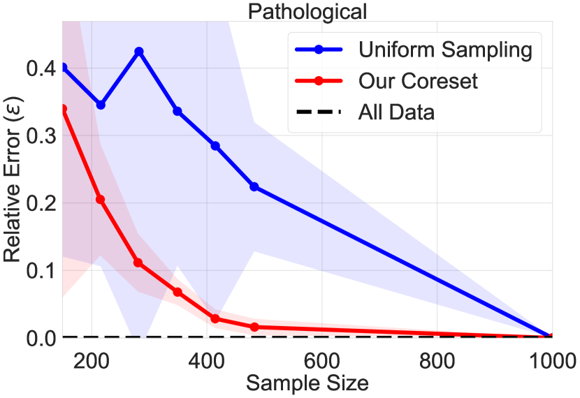
We considered 666 real-world data sets of varying size and complexity as depicted in Table 1 (also see Sec. 0.D of the Appendix). For each data set of size n𝑛n, we selected a set of M=15𝑀15M=15 geometrically-spaced subsample sizes m1,,mM[logn,n4/5]subscript𝑚1subscript𝑚M𝑛superscript𝑛45m_{1},\ldots,m_{\text{M}}\subset[\log{n},n^{4/5}]. For each sample size m𝑚m, we ran each algorithm (Alg. 1 or uniform sampling) to construct a subset SS=(S,v)SS𝑆𝑣\SS=(S,v) of size m𝑚m. We then trained the SVM model as per usual on this subset to obtain an optimal solution with respect to the coreset SSSS\SS, i.e., wSS=argminwFλ(SS,w)superscriptsubscript𝑤SSsubscript𝑤subscript𝐹𝜆SS𝑤w_{\SS}^{*}=\operatorname*{\arg\!\min}_{w}F_{\lambda}(\SS,w). We then computed the relative error incurred by the solution computed on the coreset (wSSsuperscriptsubscript𝑤SSw_{\SS}^{*}) with respect to the ground-truth optimal solution computed on the entire data set (wsuperscript𝑤w^{*}): |Fλ(P,wSS)Fλ(P,w)|/Fλ(P,w);subscript𝐹𝜆𝑃superscriptsubscript𝑤SSsubscript𝐹𝜆𝑃superscript𝑤subscript𝐹𝜆𝑃superscript𝑤\nicefrac{{\left|F_{\lambda}(P,w_{\SS}^{*})-F_{\lambda}(P,w^{*})\right|}}{{F_{\lambda}(P,w^{*})}}; See Corollary 1 at Sec. 0.A.4 of the Appendix. The results were averaged across 100100100 trials.

Refer to caption
Refer to caption
Refer to caption
Refer to caption
Refer to caption
Refer to caption
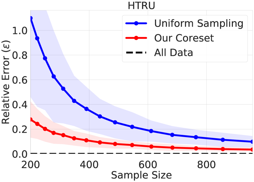
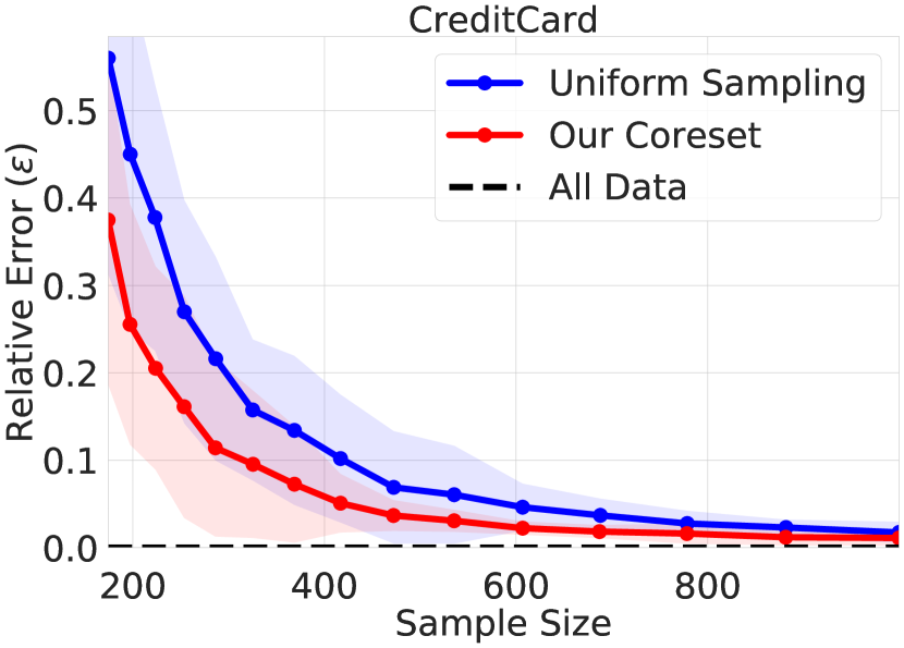
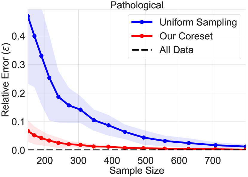
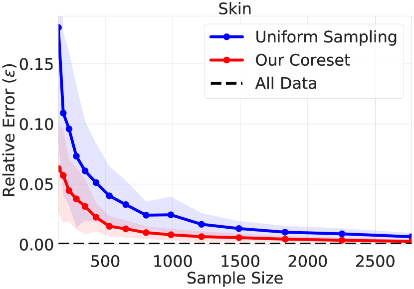
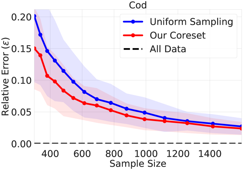
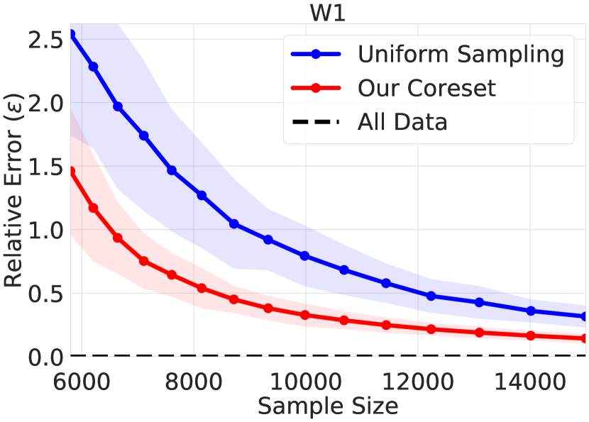
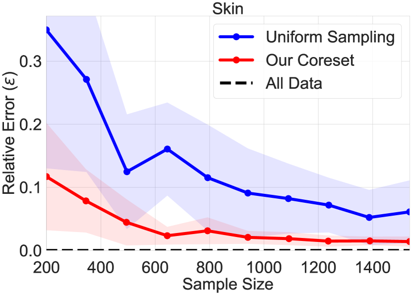
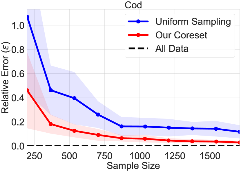
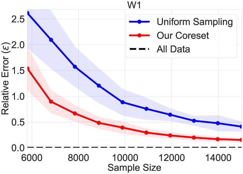
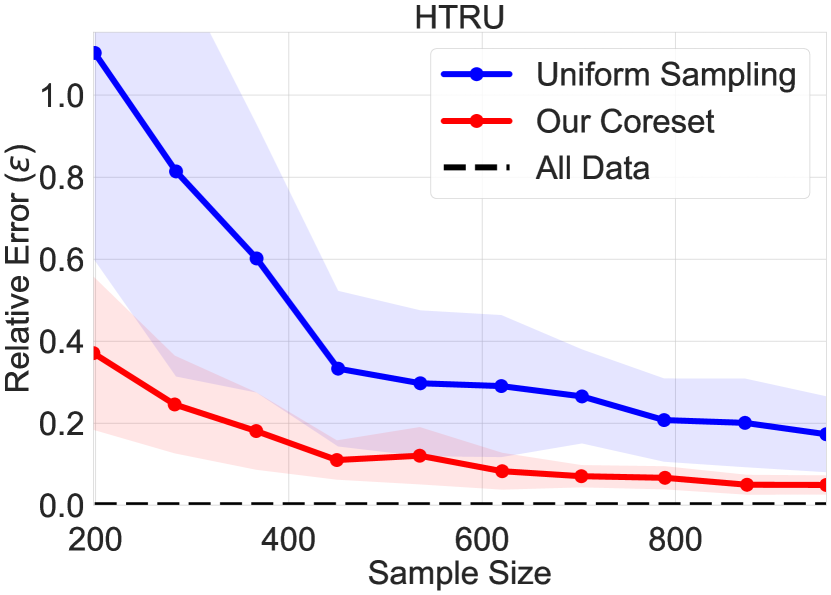
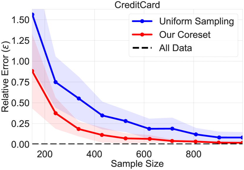
Figure 1: The relative error of query evaluations with respect uniform and coreset subsamples for the 6 data sets in the offline setting. Shaded region corresponds to values within one standard deviation of the mean.

Figures 1 and 2 depict the results of our comparisons against uniform sampling in the offline setting. In Fig. 1, we see that the coresets generated by our algorithm are much more representative and compact than the ones constructed by uniform sampling: across all data sets and sample sizes, training on our coreset yields significantly better solutions to SVM problem when compared to those generated by training on a uniform sample. For certain data sets, such as HTRU, Pathological, and W1, this relative improvement over uniform sampling is at least an order of magnitude better, especially for small sample sizes. Fig. 1 also shows that, as a consequence of a more informed sampling scheme, the variance of each model’s performance trained on our coreset is much lower than that of uniform sampling for all data sets.

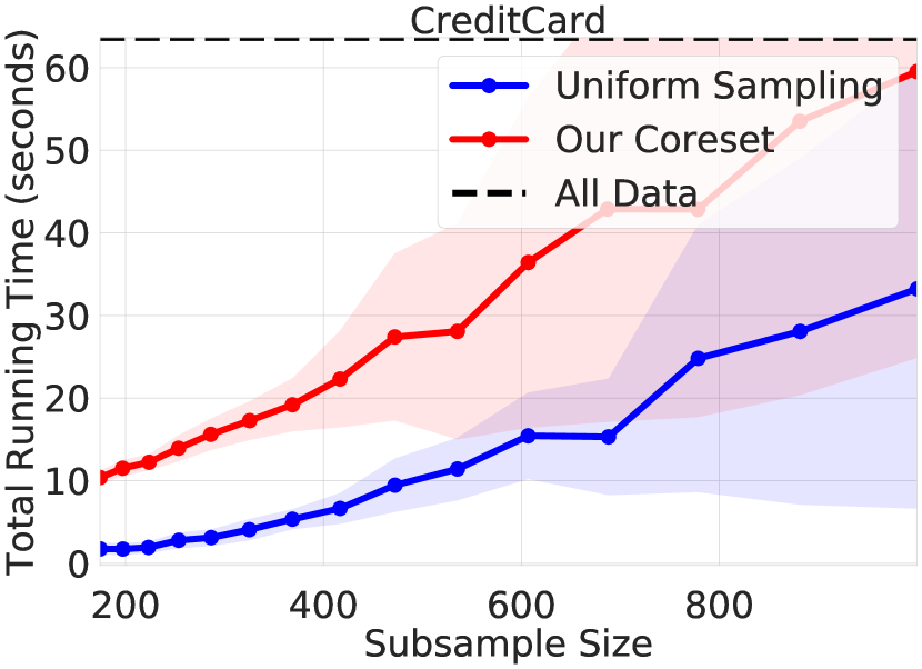
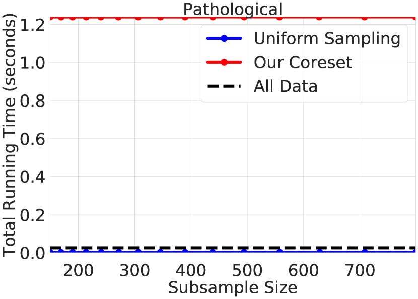
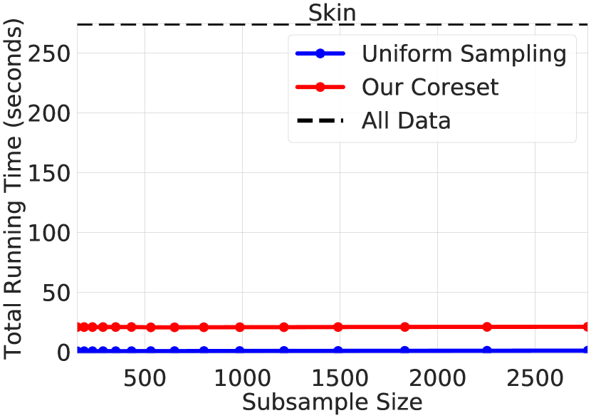
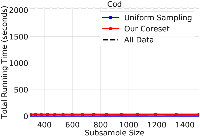
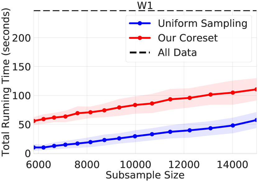
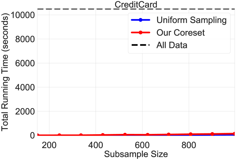
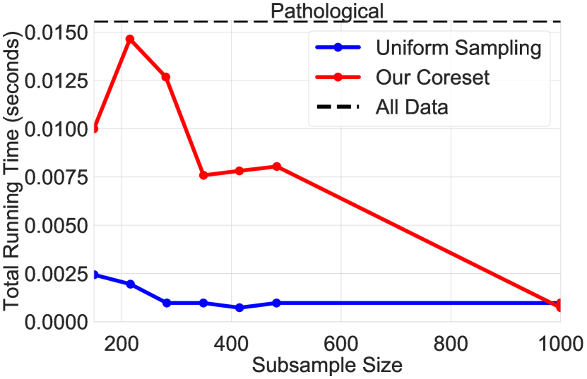
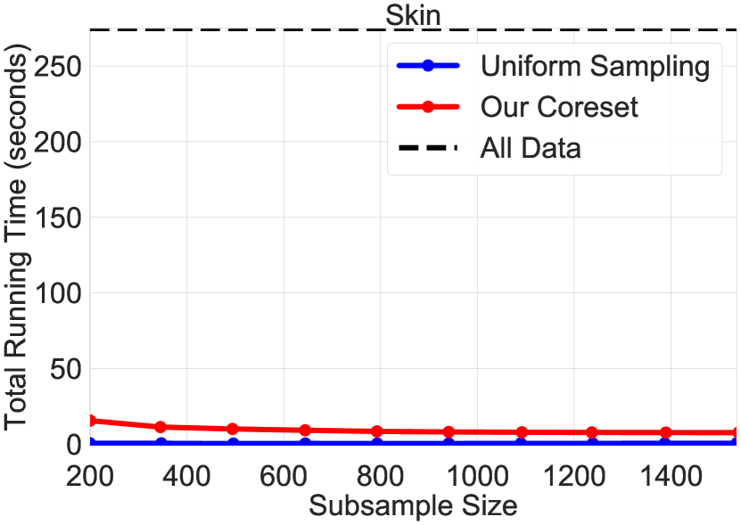
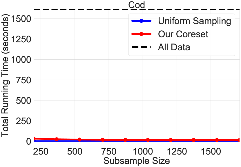
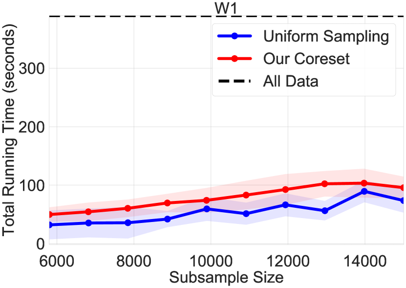
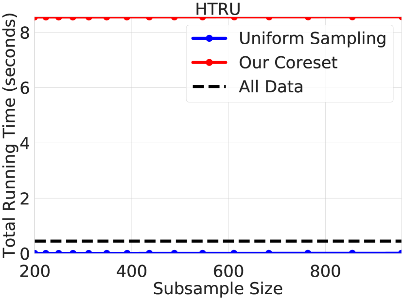
Fig. 2 shows the total computational time required for constructing the sub-sample (i.e., coreset) SSSS\SS and training the SVM on the subset SSSS\SS to obtain wSSsuperscriptsubscript𝑤SSw_{\SS}^{*}. We observe that our approach takes significantly less time than training on the original model when considering non-trivial data sets (i.e., n18,000𝑛18000n\geq 18,000), and underscores the efficiency of our method: we incur a negligible cost in the overall SVM training time due to a more involved coreset construction procedure, but benefit heavily in terms of the accuracy of the models generated (Fig. 1).
Refer to caption
Refer to caption
Refer to caption
Refer to caption
Refer to caption
Refer to caption
Figure 2: The total computational cost of constructing a coreset and training the SVM model on the coreset, plotted as a function of the size of the coreset.

Next, we evaluate our approach in the streaming setting, where data points arrive one-by-one and the entire data set cannot be kept in memory, for the same 666 data sets. The results of the streaming setting are shown in Fig. 3. The corresponding figure for the total computational time is shown as Fig. 5 in Sec. 0.E of the Appendix. Figs. 3 and 5 (in the Appendix) portray a similar trend as the one we observed in our offline evaluations: our approach significantly outperforms uniform sampling for all of the evaluated data sets and sample sizes, with negligible computational overhead.
Refer to caption
Refer to caption
Refer to caption
Refer to caption
Refer to caption
Refer to caption
Figure 3: The relative error of query evaluations with respect uniform and coreset subsamples for the 666 data sets in the streaming setting. The figure shows that our method tends to fare even better in the streaming setting (cf. Fig. 1).

In sum, our empirical evaluations demonstrate the practical efficiency of our algorithm and reaffirm the favorable theoretical guarantees of our approach: the additional computational complexity of constructing the coreset is negligible relative to that of uniform sampling, and the entire preprocess-then-train pipeline is significantly more efficient than training on the original massive data set.

7 Conclusion

We presented an efficient coreset construction algorithm for generating compact representations of the input data points that are provably competitive with the original data set in training Support Vector Machine models. Unlike prior approaches, our method and its theoretical guarantees naturally extend to streaming settings and scenarios involving dynamic data sets, where points are continuously inserted and deleted. We established instance-dependent bounds on the number of samples required to obtain accurate approximations to the SVM problem as a function of input data complexity and established dataset dependent conditions for the existence of compact representations. Our experimental results on real-world data sets validate our theoretical results and demonstrate the practical efficacy of our approach in speeding up SVM training. We conjecture that our coreset construction can be extended to accelerate SVM training for other classes of kernels and can be applied to a variety of Big Data scenarios.

References

  • [1] Agarwal, P.K., Har-Peled, S., Varadarajan, K.R.: Geometric approximation via coresets. Combinatorial and computational geometry 52, 1–30 (2005)
  • [2] Agarwal, P.K., Sharathkumar, R.: Streaming algorithms for extent problems in high dimensions. In: Proceedings of the twenty-first annual ACM-SIAM symposium on Discrete Algorithms. pp. 1481–1489. Society for Industrial and Applied Mathematics (2010)
  • [3] Arthur, D., Vassilvitskii, S.: k-means++: The advantages of careful seeding. In: Proceedings of the eighteenth annual ACM-SIAM symposium on Discrete algorithms. pp. 1027–1035. Society for Industrial and Applied Mathematics (2007)
  • [4] Bachem, O., Lucic, M., Krause, A.: Practical coreset constructions for machine learning. arXiv preprint arXiv:1703.06476 (2017)
  • [5] Badoiu, M., Clarkson, K.L.: Smaller core-sets for balls. In: Proceedings of the fourteenth annual ACM-SIAM symposium on Discrete algorithms. pp. 801–802. Society for Industrial and Applied Mathematics (2003)
  • [6] Baykal, C., Liebenwein, L., Gilitschenski, I., Feldman, D., Rus, D.: Data-dependent coresets for compressing neural networks with applications to generalization bounds. arXiv preprint arXiv:1804.05345 (2018)
  • [7] Braverman, V., Feldman, D., Lang, H.: New frameworks for offline and streaming coreset constructions. arXiv preprint arXiv:1612.00889 (2016)
  • [8] Clarkson, K.L.: Coresets, sparse greedy approximation, and the frank-wolfe algorithm. ACM Transactions on Algorithms (TALG) 6(4),  63 (2010)
  • [9] Clarkson, K.L., Hazan, E., Woodruff, D.P.: Sublinear optimization for machine learning. Journal of the ACM (JACM) 59(5),  23 (2012)
  • [10] Feldman, D.: Core-sets: An updated survey. Wiley Interdisciplinary Reviews: Data Mining and Knowledge Discovery p. e1335 (2019)
  • [11] Feldman, D., Langberg, M.: A unified framework for approximating and clustering data. In: Proceedings of the forty-third annual ACM symposium on Theory of computing. pp. 569–578. ACM (2011)
  • [12] Gärtner, B., Jaggi, M.: Coresets for polytope distance. In: Proceedings of the twenty-fifth annual symposium on Computational geometry. pp. 33–42. ACM (2009)
  • [13] Har-Peled, S., Mazumdar, S.: On coresets for k-means and k-median clustering. In: Proceedings of the thirty-sixth annual ACM symposium on Theory of computing. pp. 291–300. ACM (2004)
  • [14] Har-Peled, S., Roth, D., Zimak, D.: Maximum margin coresets for active and noise tolerant learning. In: IJCAI. pp. 836–841 (2007)
  • [15] Hazan, E., Koren, T., Srebro, N.: Beating sgd: Learning svms in sublinear time. In: Advances in Neural Information Processing Systems. pp. 1233–1241 (2011)
  • [16] Joachims, T.: Training linear svms in linear time. In: Proceedings of the 12th ACM SIGKDD international conference on Knowledge discovery and data mining. pp. 217–226. ACM (2006)
  • [17] Kodinariya, T.M., Makwana, P.R.: Review on determining number of cluster in k-means clustering. International Journal 1(6), 90–95 (2013)
  • [18] Langberg, M., Schulman, L.J.: Universal ε𝜀\varepsilon-approximators for integrals. In: Proceedings of the twenty-first annual ACM-SIAM symposium on Discrete Algorithms. pp. 598–607. SIAM (2010)
  • [19] Li, Y., Long, P.M., Srinivasan, A.: Improved bounds on the sample complexity of learning. Journal of Computer and System Sciences 62(3), 516–527 (2001)
  • [20] Lichman, M.: UCI machine learning repository (2013), http://archive.ics.uci.edu/ml
  • [21] Liebenwein, L., Baykal, C., Lang, H., Feldman, D., Rus, D.: Provable filter pruning for efficient neural networks. arXiv preprint arXiv:1911.07412 (2019)
  • [22] Loosli, G., Canu, S.: Comments on the “Core Vector Machines: Fast SVM Training on Very Large Data Sets. Journal of Machine Learning Research 8(Feb), 291–301 (2007)
  • [23] Lucic, M., Faulkner, M., Krause, A., Feldman, D.: Training mixture models at scale via coresets. arXiv preprint arXiv:1703.08110 (2017)
  • [24] Nandan, M., Khargonekar, P.P., Talathi, S.S.: Fast svm training using approximate extreme points. Journal of Machine Learning Research 15(1), 59–98 (2014)
  • [25] Nathan, V., Raghvendra, S.: Accurate streaming support vector machines. arXiv preprint arXiv:1412.2485 (2014)
  • [26] Rai, P., Daumé III, H., Venkatasubramanian, S.: Streamed learning: one-pass svms. arXiv preprint arXiv:0908.0572 (2009)
  • [27] Shalev-Shwartz, S., Singer, Y., Srebro, N., Cotter, A.: Pegasos: Primal estimated sub-gradient solver for svm. Mathematical programming 127(1), 3–30 (2011)
  • [28] Tsang, I.W., Kocsor, A., Kwok, J.T.: Simpler core vector machines with enclosing balls. In: Proceedings of the 24th international conference on Machine learning. pp. 911–918. ACM (2007)
  • [29] Tsang, I.W., Kwok, J.T., Cheung, P.M.: Core vector machines: Fast svm training on very large data sets. Journal of Machine Learning Research 6(Apr), 363–392 (2005)
  • [30] Vapnik, V.N., Vapnik, V.: Statistical learning theory, vol. 1. Wiley New York (1998)
  • [31] Yang, J., Chow, Y.L., Ré, C., Mahoney, M.W.: Weighted sgd for \\\backslashell_p regression with randomized preconditioning. arXiv preprint arXiv:1502.03571 (2017)

Appendix 0.A Proofs of the Analytical Results in Section 5

This section includes the full proofs of the technical results given in Sec. 5.

0.A.1 Proof of Lemma 5.2

\senslowerbound

*

Proof

Following [31], let n=(dd/2)𝑛binomial𝑑𝑑2n=\binom{d}{d/2} and let 𝒫=(P,u)𝒫𝑃𝑢\mathcal{P}=(P,u), where Pd+1×{±1}𝑃superscript𝑑1plus-or-minus1P\subseteq\mathbb{R}^{d+1}\times\left\{\pm 1\right\} be set of n𝑛n labeled points, and u:P1:𝑢𝑃1u:P\to 1. For every p=(x,y)P𝑝𝑥𝑦𝑃p=(x,y)\in P, where xd×{1}𝑥superscript𝑑1x\in\mathbb{R}^{d}\times\left\{1\right\} and y{±1}𝑦plus-or-minus1y\in\left\{\pm 1\right\}, among the first d𝑑d entries of x𝑥x, exactly d2𝑑2\frac{d}{2} entries are equivalent to

y2d,𝑦2𝑑y\sqrt{\frac{2}{d}},

where the remaining d2𝑑2\frac{d}{2} entries among the first d𝑑d are set to 00. Hence, for our proof to hold, we assume that P𝑃P contains all such combinations and at least one point of each label. For every p=(x,y)P𝑝𝑥𝑦𝑃p=(x,y)\in P, define the set of non-zero entries of p𝑝p as the set

Bp={i[d+1]:xi0}.subscript𝐵𝑝conditional-set𝑖delimited-[]𝑑1subscript𝑥𝑖0B_{p}=\{i\in[d+1]:x_{i}\neq 0\}.

Put pP𝑝𝑃p\in P and note that for bounding the sensitivity of point p𝑝p, consider w𝑤w with entries defined as

i[d+1]wi={0ifiBp,12dotherwise.for-all𝑖delimited-[]𝑑1subscript𝑤𝑖cases0if𝑖subscript𝐵𝑝otherwise12𝑑otherwiseotherwise\forall{i\in[d+1]}\hskip 7.11317ptw_{i}=\begin{cases}0\hskip 7.11317pt\text{if}\hskip 7.11317pti\in B_{p},\\ \frac{1}{\sqrt{\frac{2}{d}}}\hskip 7.11317pt\text{otherwise}.\end{cases}

Note that w22=d2(12d)2=d24superscriptsubscriptnorm𝑤22𝑑2superscript12𝑑2superscript𝑑24\left\|w\right\|_{2}^{2}=\frac{d}{2}\left(\frac{1}{\sqrt{\frac{2}{d}}}\right)^{2}=\frac{d^{2}}{4}. We also have that h(p,w)=1𝑝𝑤1h(p,w)=1 since yx,w=iBpyxiwi=d20=0𝑦𝑥𝑤subscript𝑖subscript𝐵𝑝𝑦subscript𝑥𝑖subscript𝑤𝑖𝑑200y\langle x,w\rangle=\sum_{i\in B_{p}}yx_{i}w_{i}=\frac{d}{2}0=0. To bound the sum of hinge losses contributed by other points qP{p}𝑞𝑃𝑝q\in P\setminus\left\{p\right\}, note that BqBpsubscript𝐵𝑞subscript𝐵𝑝B_{q}\setminus B_{p}\neq\emptyset. Then for every q=(x,y)p𝑞superscript𝑥superscript𝑦𝑝q=(x^{\prime},y^{\prime})\neq p,

yx,wsuperscript𝑦superscript𝑥𝑤\displaystyle y^{\prime}\langle x^{\prime},w\rangle =iBqBpyxiwi12d2d=1,absentsubscript𝑖subscript𝐵𝑞subscript𝐵𝑝superscript𝑦subscriptsuperscript𝑥𝑖subscript𝑤𝑖12𝑑2𝑑1\displaystyle=\sum_{i\in B_{q}\setminus B_{p}}y^{\prime}x^{\prime}_{i}w_{i}\geq\frac{1}{\sqrt{\frac{2}{d}}}\sqrt{\frac{2}{d}}=1,

which implies that h(q,w)=0𝑞𝑤0h(q,w)=0. Thus,

qPh(q,w)=1.subscript𝑞𝑃𝑞𝑤1\sum_{q\in P}h(q,w)=1.

Putting it all together,

s(p)=supwd+1Fλ(𝒫,w)0fλ(p,w)Fλ(𝒫,w)d28n+λh(p,w)w222+λ=d28n+λd28+λ.𝑠𝑝subscriptsupremumsuperscript𝑤superscript𝑑1subscript𝐹𝜆𝒫superscript𝑤0subscript𝑓𝜆𝑝superscript𝑤subscript𝐹𝜆𝒫superscript𝑤superscript𝑑28𝑛𝜆𝑝𝑤superscriptsubscriptnorm𝑤222𝜆superscript𝑑28𝑛𝜆superscript𝑑28𝜆\displaystyle s(p)=\sup_{\begin{subarray}{c}w^{\prime}\in\mathbb{R}^{d+1}\\ F_{\lambda}(\mathcal{P},w^{\prime})\neq 0\end{subarray}}\frac{f_{\lambda}(p,w^{\prime})}{F_{\lambda}(\mathcal{P},w^{\prime})}\geq\frac{\frac{d^{2}}{8n}+\lambda\,h(p,w)}{\frac{\left\|w\right\|_{2}^{2}}{2}+\lambda}=\frac{\frac{d^{2}}{8n}+\lambda}{\frac{d^{2}}{8}+\lambda}.

Since the above holds for every pP𝑝𝑃p\in P, summing the above inequality over every pP𝑝𝑃p\in P, yields that

pPs(p)d28+nλd28+λΩ(d2+nλd2+λ).subscript𝑝𝑃𝑠𝑝superscript𝑑28𝑛𝜆superscript𝑑28𝜆Ωsuperscript𝑑2𝑛𝜆superscript𝑑2𝜆\displaystyle\sum_{p\in P}s(p)\geq\frac{\frac{d^{2}}{8}+n\lambda}{\frac{d^{2}}{8}+\lambda}\in\Omega\left(\frac{d^{2}+n\lambda}{d^{2}+\lambda}\right).

0.A.2 Proof of Lemma 5.3

\sensupperbound

*

Proof

Let PyPsubscript𝑃𝑦𝑃P_{y}\subseteq P denote the set of points with the same label as p𝑝p as in Line 1 of Algorithm 1. Consider an optimal clustering of the points in Pysubscript𝑃𝑦P_{y} into k𝑘k clusters with centroids 𝒞y={cy(1),,cy(k)}d+1superscript𝒞𝑦superscriptsubscript𝑐𝑦1superscriptsubscript𝑐𝑦𝑘superscript𝑑1\mathcal{C}^{y}=\{c_{y}^{(1)},\ldots,c_{y}^{(k)}\}\subseteq\mathbb{R}^{d+1} being their mean as in Line 1, and let αy(i)superscriptsubscript𝛼𝑦𝑖\alpha_{y}^{(i)} be as defined in Line 1 for every i[k]𝑖delimited-[]𝑘i\in[k] and y{+,}𝑦y\in\left\{+,-\right\}. In addition, let 𝒫𝒫y(i)𝒫superscriptsubscript𝒫𝑦𝑖\mathcal{P}\setminus\mathcal{P}_{y}^{(i)} denote the weighted set (PPy(i),u)𝑃superscriptsubscript𝑃𝑦𝑖𝑢\left(P\setminus P_{y}^{(i)},u\right) for every i[k]𝑖delimited-[]𝑘i\in[k] and y{+,}𝑦y\in\left\{+,-\right\}.

Put p=(x,y)P𝑝𝑥𝑦𝑃p=(x,y)\in P and let i[k]𝑖delimited-[]𝑘i\in[k] be the index of the cluster which p𝑝p belongs to, i.e., pPy(i)𝑝superscriptsubscript𝑃𝑦𝑖p\in P_{y}^{(i)}.

We first observe that for any scalars a,b𝑎𝑏a,b\in\mathbb{R}, max{ab,0}max{a,0}+max{b,0}𝑎𝑏0𝑎0𝑏0\max\{a-b,0\}\leq\max\{a,0\}+\max\{-b,0\}. This implies that, by definition of the hinge loss, we have for every q,q^,wd+1𝑞^𝑞𝑤superscript𝑑1q,\hat{q},w\in\mathbb{R}^{d+1}

h(q,w)h(q^,w)+[qq^,w]+,𝑞𝑤^𝑞𝑤subscriptdelimited-[]𝑞^𝑞𝑤h(q,w)\leq h(\hat{q},w)+\left[\langle q-\hat{q},w\rangle\right]_{+},

where [x]+=max{0,x}subscriptdelimited-[]𝑥0𝑥\left[x\right]_{+}=\max\{0,x\} as before. Hence, in the context of the definitions above

h(p,w)𝑝𝑤\displaystyle h(p,w) =h(pc(p)+c(p),w)absent𝑝𝑐𝑝𝑐𝑝𝑤\displaystyle=h(p-c(p)+c(p),w) (5)
h(c(p),w)+[c(p)yx,w]+absent𝑐𝑝𝑤subscriptdelimited-[]𝑐𝑝𝑦𝑥𝑤\displaystyle\leq h(c(p),w)+\left[\langle c(p)-yx,w\rangle\right]_{+} (6)
=h(c(p),w)+[pΔ,w]+.absent𝑐𝑝𝑤subscriptdelimited-[]subscript𝑝Δ𝑤\displaystyle=h(c(p),w)+\left[\langle p_{\Delta},w\rangle\right]_{+}. (7)

Now let the total weight of the points in Py(i)superscriptsubscript𝑃𝑦𝑖P_{y}^{(i)} be denoted by U(Py(i))=qPy(i)u(q)𝑈superscriptsubscript𝑃𝑦𝑖subscript𝑞superscriptsubscript𝑃𝑦𝑖𝑢𝑞U{\left(P_{y}^{(i)}\right)}=\sum\limits_{q\in P_{y}^{(i)}}u(q). Note that since cy(i)superscriptsubscript𝑐𝑦𝑖c_{y}^{(i)} is the centroid of Py(i)superscriptsubscript𝑃𝑦𝑖P_{y}^{(i)} (as described in Line 1 of Algorithm 1), we have Py(i)=1U(Py(i))q=(xq,yq)Py(i)u(q)yqxq.superscriptsubscript𝑃𝑦𝑖1𝑈superscriptsubscript𝑃𝑦𝑖subscript𝑞subscript𝑥𝑞subscript𝑦𝑞superscriptsubscript𝑃𝑦𝑖𝑢𝑞subscript𝑦𝑞subscript𝑥𝑞P_{y}^{(i)}=\frac{1}{U{\left(P_{y}^{(i)}\right)}}\sum\limits_{q=(x_{q},y_{q})\in P_{y}^{(i)}}u(q)y_{q}x_{q}. Observing that the hinge loss is convex, we invoke Jensen’s inequality to obtain

fλ(cy(i),w)1U(Py(i))qPy(i)u(q)f(q,w)=Fλ(𝒫,w)Fλ(𝒫𝒫y(i),w)U(Py(i)).subscript𝑓𝜆superscriptsubscript𝑐𝑦𝑖𝑤1𝑈superscriptsubscript𝑃𝑦𝑖subscript𝑞superscriptsubscript𝑃𝑦𝑖𝑢𝑞𝑓𝑞𝑤subscript𝐹𝜆𝒫𝑤subscript𝐹𝜆𝒫superscriptsubscript𝒫𝑦𝑖𝑤𝑈superscriptsubscript𝑃𝑦𝑖f_{\lambda}(c_{y}^{(i)},w)\leq\frac{1}{U{\left(P_{y}^{(i)}\right)}}\sum_{q\in P_{y}^{(i)}}u(q)f(q,w)=\frac{F_{\lambda}(\mathcal{P},w)-F_{\lambda}(\mathcal{P}\setminus\mathcal{P}_{y}^{(i)},w)}{U{\left(P_{y}^{(i)}\right)}}.

Applying the two inequalities established above to s(p)/u(p)𝑠𝑝𝑢𝑝s(p)/u(p) yields that

s(p)u(p)𝑠𝑝𝑢𝑝\displaystyle\frac{s(p)}{u(p)} =supwfλ(p,w)Fλ(𝒫,w)absentsubscriptsupremum𝑤subscript𝑓𝜆𝑝𝑤subscript𝐹𝜆𝒫𝑤\displaystyle=\sup_{w}\frac{f_{\lambda}(p,w)}{F_{\lambda}(\mathcal{P},w)} (8)
supwfλ(cy(i),w)+λ[w,pΔ]+Fλ(𝒫,w)absentsubscriptsupremum𝑤subscript𝑓𝜆superscriptsubscript𝑐𝑦𝑖𝑤𝜆subscriptdelimited-[]𝑤subscript𝑝Δsubscript𝐹𝜆𝒫𝑤\displaystyle\leq\sup_{w}\frac{f_{\lambda}(c_{y}^{(i)},w)+\lambda\left[\langle w,p_{\Delta}\rangle\right]_{+}}{F_{\lambda}(\mathcal{P},w)} (9)
supwqPy(i)u(q)fλ(q,w)U(Py(i))Fλ(𝒫,w)+λ[w,pΔ]+Fλ(𝒫,w)absentsubscriptsupremum𝑤subscript𝑞superscriptsubscript𝑃𝑦𝑖𝑢𝑞subscript𝑓𝜆𝑞𝑤𝑈superscriptsubscript𝑃𝑦𝑖subscript𝐹𝜆𝒫𝑤𝜆subscriptdelimited-[]𝑤subscript𝑝Δsubscript𝐹𝜆𝒫𝑤\displaystyle\leq\sup_{w}\frac{\sum\limits_{q\in P_{y}^{(i)}}u(q)f_{\lambda}(q,w)}{U{\left(P_{y}^{(i)}\right)}F_{\lambda}(\mathcal{P},w)}+\frac{\lambda\left[\langle w,p_{\Delta}\rangle\right]_{+}}{F_{\lambda}(\mathcal{P},w)} (10)
=supwFλ(𝒫,w)Fλ(𝒫𝒫y(i),w)U(Py(i))Fλ(𝒫,w)+λ[w,pΔ]+Fλ(𝒫,w)absentsubscriptsupremum𝑤subscript𝐹𝜆𝒫𝑤subscript𝐹𝜆𝒫superscriptsubscript𝒫𝑦𝑖𝑤𝑈superscriptsubscript𝑃𝑦𝑖subscript𝐹𝜆𝒫𝑤𝜆subscriptdelimited-[]𝑤subscript𝑝Δsubscript𝐹𝜆𝒫𝑤\displaystyle=\sup_{w}\frac{F_{\lambda}(\mathcal{P},w)-F_{\lambda}(\mathcal{P}\setminus\mathcal{P}_{y}^{(i)},w)}{U{\left(P_{y}^{(i)}\right)}F_{\lambda}(\mathcal{P},w)}+\frac{\lambda\left[\langle w,p_{\Delta}\rangle\right]_{+}}{F_{\lambda}(\mathcal{P},w)} (11)
=1U(Py(i))+supwλ[w,pΔ]+Fλ(PPy(i),w)/U(Py(i))Fλ(𝒫,w)absent1𝑈superscriptsubscript𝑃𝑦𝑖subscriptsupremum𝑤𝜆subscriptdelimited-[]𝑤subscript𝑝Δsubscript𝐹𝜆𝑃superscriptsubscript𝑃𝑦𝑖𝑤𝑈superscriptsubscript𝑃𝑦𝑖subscript𝐹𝜆𝒫𝑤\displaystyle=\frac{1}{U{\left(P_{y}^{(i)}\right)}}+\sup_{w}\frac{\lambda\left[\langle w,p_{\Delta}\rangle\right]_{+}-F_{\lambda}(P\setminus P_{y}^{(i)},w)/U{\left(P_{y}^{(i)}\right)}}{F_{\lambda}(\mathcal{P},w)} (12)

By definition of Fλ(PPy(i),w)subscript𝐹𝜆𝑃superscriptsubscript𝑃𝑦𝑖𝑤F_{\lambda}(P\setminus P_{y}^{(i)},w), we have

Fλ(PPy(i),w)w1:d22U(PPy(i))2U(P).subscript𝐹𝜆𝑃superscriptsubscript𝑃𝑦𝑖𝑤superscriptsubscriptnormsubscript𝑤:1𝑑22𝑈𝑃superscriptsubscript𝑃𝑦𝑖2𝑈𝑃\displaystyle F_{\lambda}(P\setminus P_{y}^{(i)},w)\geq\frac{\left\|w_{1:d}\right\|_{2}^{2}\,U{\left(P\setminus P_{y}^{(i)}\right)}}{2U{\left(P\right)}}.

Continuing from above and dividing both sides by λ𝜆\lambda yields

s(p)λu(p)𝑠𝑝𝜆𝑢𝑝\displaystyle\frac{s(p)}{\lambda u(p)} 1λU(Py(i))+supw[w,pΔ]+w1:d2U(PPy(i))2λU(P)U(Py(i))Fλ(𝒫,w)absent1𝜆𝑈superscriptsubscript𝑃𝑦𝑖subscriptsupremum𝑤subscriptdelimited-[]𝑤subscript𝑝Δsuperscriptnormsubscript𝑤:1𝑑2𝑈𝑃superscriptsubscript𝑃𝑦𝑖2𝜆𝑈𝑃𝑈superscriptsubscript𝑃𝑦𝑖subscript𝐹𝜆𝒫𝑤\displaystyle\leq\frac{1}{\lambda U{\left(P_{y}^{(i)}\right)}}+\sup_{w}\frac{\left[\langle w,p_{\Delta}\rangle\right]_{+}-\frac{\left\|w_{1:d}\right\|^{2}\,U{\left(P\setminus P_{y}^{(i)}\right)}}{2\lambda U{\left(P\right)}U{\left(P_{y}^{(i)}\right)}}}{F_{\lambda}(\mathcal{P},w)}
1λu(𝒞p)+supw[w,pΔ]+αy(i)w1:d22Fλ(𝒫,w),absent1𝜆𝑢subscript𝒞𝑝subscriptsupremum𝑤subscriptdelimited-[]𝑤subscript𝑝Δsuperscriptsubscript𝛼𝑦𝑖superscriptsubscriptnormsubscript𝑤:1𝑑22subscript𝐹𝜆𝒫𝑤\displaystyle\leq\frac{1}{\lambda u(\mathcal{C}_{p})}+\sup_{w}\frac{\left[\langle w,p_{\Delta}\rangle\right]_{+}-\alpha_{y}^{(i)}\left\|w_{1:d}\right\|_{2}^{2}}{F_{\lambda}(\mathcal{P},w)},

where

αy(i)=U(PPy(i))2λU(P)U(Py(i)).superscriptsubscript𝛼𝑦𝑖𝑈𝑃superscriptsubscript𝑃𝑦𝑖2𝜆𝑈𝑃𝑈superscriptsubscript𝑃𝑦𝑖\alpha_{y}^{(i)}=\frac{U{\left(P\setminus P_{y}^{(i)}\right)}}{2\lambda U{\left(P\right)}U{\left(P_{y}^{(i)}\right)}}. (13)

Let

g(w)=[w,pΔ]+αy(i)w1:d22Fλ(𝒫,w)𝑔𝑤subscriptdelimited-[]𝑤subscript𝑝Δsuperscriptsubscript𝛼𝑦𝑖superscriptsubscriptnormsubscript𝑤:1𝑑22subscript𝐹𝜆𝒫𝑤g(w)=\frac{\left[\langle w,p_{\Delta}\rangle\right]_{+}-\alpha_{y}^{(i)}\left\|w_{1:d}\right\|_{2}^{2}}{F_{\lambda}(\mathcal{P},w)}

be the expression on the right hand side of the sensitivity inequality above, and let w^argmaxwg(w)^𝑤subscript𝑤𝑔𝑤\hat{w}\in\operatorname*{\arg\!\max}_{w}g(w). The rest of the proof will focus on bounding g(w^)𝑔^𝑤g(\hat{w}), since an upper bound on the sensitivity of a point as a whole would follow directly from an upper bound on g(w^)𝑔^𝑤g(\hat{w}).

Note that by definition of pΔsubscript𝑝Δp_{\Delta} and the embedding of 111 to the (d+1)thsuperscript𝑑1th(d+1)^{\text{th}} entry of the original d𝑑d-dimensional point (with respect to p𝑝p),

w^,pΔ=w^1:d,(pΔ)1:d,^𝑤subscript𝑝Δsubscript^𝑤:1𝑑subscriptsubscript𝑝Δ:1𝑑\langle\hat{w},p_{\Delta}\rangle=\langle\hat{w}_{1:d},(p_{\Delta})_{1:d}\rangle,

where the equality holds since the (d+1)𝑑1(d+1)th entry of pΔsubscript𝑝Δp_{\Delta} is zero.

We know that w^,pΔαy(i)w^1:d220^𝑤subscript𝑝Δsuperscriptsubscript𝛼𝑦𝑖superscriptsubscriptnormsubscript^𝑤:1𝑑220\langle\hat{w},p_{\Delta}\rangle\geq\alpha_{y}^{(i)}\left\|\hat{w}_{1:d}\right\|_{2}^{2}\geq 0, since otherwise g(w^)<0𝑔^𝑤0g(\hat{w})<0, which contradicts the fact that w^^𝑤\hat{w} is the maximizer of g(w)𝑔𝑤g(w). This implies that for each entry j[d]𝑗delimited-[]𝑑j\in[d] of the sub-gradient of g()𝑔g(\cdot) evaluated at w^^𝑤\hat{w}, denoted by g(w^)𝑔^𝑤\nabla g(\hat{w}), is given by

g(w^)j𝑔subscript^𝑤𝑗\displaystyle\nabla g(\hat{w})_{j} =((pΔ)j2αy(i)w^j)Fλ(𝒫,w^)Fλ(𝒫,w^)j(w,pΔαy(i)w1:d22)Fλ(𝒫,w^)2,absentsubscriptsubscript𝑝Δ𝑗2superscriptsubscript𝛼𝑦𝑖subscript^𝑤𝑗subscript𝐹𝜆𝒫^𝑤subscript𝐹𝜆subscript𝒫^𝑤𝑗𝑤subscript𝑝Δsuperscriptsubscript𝛼𝑦𝑖superscriptsubscriptnormsubscript𝑤:1𝑑22subscript𝐹𝜆superscript𝒫^𝑤2\displaystyle=\frac{\left((p_{\Delta})_{j}-2\alpha_{y}^{(i)}\hat{w}_{j}\right)F_{\lambda}(\mathcal{P},\hat{w})-\nabla F_{\lambda}(\mathcal{P},\hat{w})_{j}\left(\langle w,p_{\Delta}\rangle-\alpha_{y}^{(i)}\left\|w_{1:d}\right\|_{2}^{2}\right)}{{F_{\lambda}(\mathcal{P},\hat{w})}^{2}}, (14)

and that g(w^)d+1=0𝑔subscript^𝑤𝑑10\nabla g(\hat{w})_{d+1}=0 since the bias term does not appear in the numerator of g()𝑔g(\cdot).

Letting γ=w^,pΔαy(i)w^1:d22𝛾^𝑤subscript𝑝Δsuperscriptsubscript𝛼𝑦𝑖superscriptsubscriptnormsubscript^𝑤:1𝑑22\gamma=\langle\hat{w},p_{\Delta}\rangle-\alpha_{y}^{(i)}\left\|\hat{w}_{1:d}\right\|_{2}^{2} and setting each entry of the gradient g(w^)𝑔^𝑤\nabla g(\hat{w}) to 00, we solve for pΔsubscript𝑝Δp_{\Delta} to obtain

(pΔ)1:d=γFλ(𝒫,w^)1:dFλ(𝒫,w^)+2αy(i)w^1:d.subscriptsubscript𝑝Δ:1𝑑𝛾subscript𝐹𝜆subscript𝒫^𝑤:1𝑑subscript𝐹𝜆𝒫^𝑤2superscriptsubscript𝛼𝑦𝑖subscript^𝑤:1𝑑(p_{\Delta})_{1:d}=\frac{\gamma\,\nabla F_{\lambda}(\mathcal{P},\hat{w})_{1:d}}{F_{\lambda}(\mathcal{P},\hat{w})}+2\alpha_{y}^{(i)}\hat{w}_{1:d}.

This implies that

w^,pΔ^𝑤subscript𝑝Δ\displaystyle\langle\hat{w},p_{\Delta}\rangle =γw^,Fλ(𝒫,w^)Fλ(𝒫,w^)+2αy(i)w^1:d22absent𝛾^𝑤subscript𝐹𝜆𝒫^𝑤subscript𝐹𝜆𝒫^𝑤2superscriptsubscript𝛼𝑦𝑖superscriptsubscriptnormsubscript^𝑤:1𝑑22\displaystyle=\frac{\gamma\,\langle\hat{w},\nabla F_{\lambda}(\mathcal{P},\hat{w})\rangle}{F_{\lambda}(\mathcal{P},\hat{w})}+2\alpha_{y}^{(i)}\left\|\hat{w}_{1:d}\right\|_{2}^{2}

Rearranging and using the definition of γ𝛾\gamma, we obtain

γ=γw^,Fλ(𝒫,w^)Fλ(𝒫,w^)+αy(i)w^1:d22,𝛾𝛾^𝑤subscript𝐹𝜆𝒫^𝑤subscript𝐹𝜆𝒫^𝑤superscriptsubscript𝛼𝑦𝑖superscriptsubscriptnormsubscript^𝑤:1𝑑22\gamma=\frac{\gamma\,\langle\hat{w},\nabla F_{\lambda}(\mathcal{P},\hat{w})\rangle}{F_{\lambda}(\mathcal{P},\hat{w})}+\alpha_{y}^{(i)}\left\|\hat{w}_{1:d}\right\|_{2}^{2}, (15)

where Lemma 5.3 holds by taking 9292\frac{9}{2} outside the max term.

By using the same equivalency for pΔsubscript𝑝Δp_{\Delta} from above, we also obtain that

pΔ22superscriptsubscriptnormsubscript𝑝Δ22\displaystyle\left\|p_{\Delta}\right\|_{2}^{2} =pΔ,pΔ=γFλ(𝒫,w^)1:dFλ(𝒫,w^)+2αy(i)w^2absentsubscript𝑝Δsubscript𝑝Δsuperscriptnorm𝛾subscript𝐹𝜆subscript𝒫^𝑤:1𝑑subscript𝐹𝜆𝒫^𝑤2superscriptsubscript𝛼𝑦𝑖^𝑤2\displaystyle=\langle p_{\Delta},p_{\Delta}\rangle=\left\|\frac{\gamma\,\nabla F_{\lambda}(\mathcal{P},\hat{w})_{1:d}}{F_{\lambda}(\mathcal{P},\hat{w})}+2\alpha_{y}^{(i)}\hat{w}\right\|^{2}
=γ2Fλ(𝒫,w^)2Fλ(𝒫,w^)22+4(αy(i))2w^1:d22+4αy(i)γw^,Fλ(𝒫,w^)Fλ(𝒫,w^),absentsuperscript𝛾2subscript𝐹𝜆superscript𝒫^𝑤2superscriptsubscriptnormsubscript𝐹𝜆𝒫^𝑤224superscriptsuperscriptsubscript𝛼𝑦𝑖2superscriptsubscriptnormsubscript^𝑤:1𝑑224superscriptsubscript𝛼𝑦𝑖𝛾^𝑤subscript𝐹𝜆𝒫^𝑤subscript𝐹𝜆𝒫^𝑤\displaystyle=\frac{\gamma^{2}}{F_{\lambda}(\mathcal{P},\hat{w})^{2}}\left\|\nabla F_{\lambda}(\mathcal{P},\hat{w})\right\|_{2}^{2}+4\left(\alpha_{y}^{(i)}\right)^{2}\left\|\hat{w}_{1:d}\right\|_{2}^{2}+4\alpha_{y}^{(i)}\frac{\gamma\,\langle\hat{w},\nabla F_{\lambda}(\mathcal{P},\hat{w})\rangle}{F_{\lambda}(\mathcal{P},\hat{w})},

but γw^,Fλ(𝒫,w^)Fλ(𝒫,w^)=γαy(i)w^1:d22𝛾^𝑤subscript𝐹𝜆𝒫^𝑤subscript𝐹𝜆𝒫^𝑤𝛾superscriptsubscript𝛼𝑦𝑖superscriptsubscriptnormsubscript^𝑤:1𝑑22\frac{\gamma\,\langle\hat{w},\nabla F_{\lambda}(\mathcal{P},\hat{w})\rangle}{F_{\lambda}(\mathcal{P},\hat{w})}=\gamma-\alpha_{y}^{(i)}\left\|\hat{w}_{1:d}\right\|_{2}^{2}, and so continuing from above, we have

pΔ22superscriptsubscriptnormsubscript𝑝Δ22\displaystyle\left\|p_{\Delta}\right\|_{2}^{2} =γ2Fλ(𝒫,w^)2Fλ(𝒫,w^)22+4(αy(i))2w^1:d22+4αy(i)(γαy(i)w^1:d22)absentsuperscript𝛾2subscript𝐹𝜆superscript𝒫^𝑤2superscriptsubscriptnormsubscript𝐹𝜆𝒫^𝑤224superscriptsuperscriptsubscript𝛼𝑦𝑖2superscriptsubscriptnormsubscript^𝑤:1𝑑224superscriptsubscript𝛼𝑦𝑖𝛾superscriptsubscript𝛼𝑦𝑖superscriptsubscriptnormsubscript^𝑤:1𝑑22\displaystyle=\frac{\gamma^{2}}{F_{\lambda}(\mathcal{P},\hat{w})^{2}}\left\|\nabla F_{\lambda}(\mathcal{P},\hat{w})\right\|_{2}^{2}+4\left(\alpha_{y}^{(i)}\right)^{2}\left\|\hat{w}_{1:d}\right\|_{2}^{2}+4\alpha_{y}^{(i)}(\gamma-\alpha_{y}^{(i)}\left\|\hat{w}_{1:d}\right\|_{2}^{2})
=γ2Fλ(𝒫,w^)2Fλ(𝒫,w^)1:d22+4αy(i)γabsentsuperscript𝛾2subscript𝐹𝜆superscript𝒫^𝑤2superscriptsubscriptnormsubscript𝐹𝜆subscript𝒫^𝑤:1𝑑224superscriptsubscript𝛼𝑦𝑖𝛾\displaystyle=\frac{\gamma^{2}}{F_{\lambda}(\mathcal{P},\hat{w})^{2}}\left\|\nabla F_{\lambda}(\mathcal{P},\hat{w})_{1:d}\right\|_{2}^{2}+4\alpha_{y}^{(i)}\gamma
=γ2x~+4αy(i)γ,absentsuperscript𝛾2~𝑥4superscriptsubscript𝛼𝑦𝑖𝛾\displaystyle=\gamma^{2}\tilde{x}+4\alpha_{y}^{(i)}\gamma,

where x~=Fλ(𝒫,w^)22Fλ(𝒫,w^)2~𝑥superscriptsubscriptnormsubscript𝐹𝜆𝒫^𝑤22subscript𝐹𝜆superscript𝒫^𝑤2\tilde{x}=\frac{\left\|\nabla F_{\lambda}(\mathcal{P},\hat{w})\right\|_{2}^{2}}{F_{\lambda}(\mathcal{P},\hat{w})^{2}}. Solving for γ𝛾\gamma from the above equation yields for x~>0~𝑥0\tilde{x}>0

γ=4(αy(i))2+pΔ2x~2αy(i)x~.𝛾4superscriptsuperscriptsubscript𝛼𝑦𝑖2superscriptnormsubscript𝑝Δ2~𝑥2superscriptsubscript𝛼𝑦𝑖~𝑥\gamma=\frac{\sqrt{4\left(\alpha_{y}^{(i)}\right)^{2}+\left\|p_{\Delta}\right\|^{2}\tilde{x}}-2\alpha_{y}^{(i)}}{\tilde{x}}. (16)

Now we subdivide the rest of the proof into two cases. The first is the trivial case in which the sensitivity of the point is sufficiently small enough to be negligible, and the second case is the involved case in which the point has a high influence on the SVM cost function and its contribution cannot be captured by the optimal solution wsuperscript𝑤w^{*} or something close to it.

Case g(w^)3αy(i)𝑔^𝑤3superscriptsubscript𝛼𝑦𝑖g(\hat{w})\leq 3\alpha_{y}^{(i)}

the bound on the sensitivity follows trivially from the analysis above.

Case g(w^)>3αy(i)𝑔^𝑤3superscriptsubscript𝛼𝑦𝑖g(\hat{w})>3\alpha_{y}^{(i)}

note that the assumption of this case implies that wsuperscript𝑤w^{*} cannot be the maximizer of g()𝑔g(\cdot), i.e., w^w^𝑤superscript𝑤\hat{w}\neq w^{*}. This follows by the convexity of the SVM loss function which implies that the norm of the gradient evaluated at wsuperscript𝑤w^{*} is 0. Thus by (15):

γ=αy(i)w1:d22.𝛾superscriptsubscript𝛼𝑦𝑖superscriptsubscriptnormsubscriptsuperscript𝑤:1𝑑22\gamma=\alpha_{y}^{(i)}\left\|{w^{*}}_{1:d}\right\|_{2}^{2}.

Since Fλ(𝒫,w)w1:d22/2subscript𝐹𝜆𝒫superscript𝑤superscriptsubscriptnormsubscriptsuperscript𝑤:1𝑑222F_{\lambda}(\mathcal{P},w^{*})\geq\left\|{w^{*}}_{1:d}\right\|_{2}^{2}/2, we obtain

s(p)αy(i)w1:d22Fλ(𝒫,w)2αy(i).𝑠𝑝superscriptsubscript𝛼𝑦𝑖superscriptsubscriptnormsubscriptsuperscript𝑤:1𝑑22subscript𝐹𝜆𝒫superscript𝑤2superscriptsubscript𝛼𝑦𝑖s(p)\leq\frac{\alpha_{y}^{(i)}\left\|{w^{*}}_{1:d}\right\|_{2}^{2}}{F_{\lambda}(\mathcal{P},w^{*})}\leq 2\alpha_{y}^{(i)}.

Hence, we know that for this case we have Fλ(𝒫,w^)2>0subscriptnormsubscript𝐹𝜆𝒫^𝑤20\left\|\nabla F_{\lambda}(\mathcal{P},\hat{w})\right\|_{2}>0, Fλ(𝒫,w^)>Fλ(𝒫,w)0subscript𝐹𝜆𝒫^𝑤subscript𝐹𝜆𝒫superscript𝑤0F_{\lambda}(\mathcal{P},\hat{w})>F_{\lambda}(\mathcal{P},w^{*})\geq 0, and so we obtain x~>0~𝑥0\tilde{x}>0.

This implies that we can use Eq.(16) to upper bound the numerator γ𝛾\gamma of the sensitivity. Note that γ𝛾\gamma from (16) is decreasing as a function of x~~𝑥\tilde{x}, and so it suffices to obtain a lower bound on x~~𝑥\tilde{x}. To do so, lets focus on Eq.(15) and let divide both sides of it by γ𝛾\gamma, to obtain that

1=w^,Fλ(𝒫,w^)Fλ(𝒫,w^)+αy(i)γw1:d22.1^𝑤subscript𝐹𝜆𝒫^𝑤subscript𝐹𝜆𝒫^𝑤superscriptsubscript𝛼𝑦𝑖𝛾superscriptsubscriptnormsubscript𝑤:1𝑑221=\frac{\langle\hat{w},\nabla F_{\lambda}(\mathcal{P},\hat{w})\rangle}{F_{\lambda}(\mathcal{P},\hat{w})}+\frac{\alpha_{y}^{(i)}}{\gamma}\left\|w_{1:d}\right\|_{2}^{2}.

By rearranging the above equality, we have that

w^,Fλ(𝒫,w^)Fλ(𝒫,w^)=1αy(i)w1:d22γ.^𝑤subscript𝐹𝜆𝒫^𝑤subscript𝐹𝜆𝒫^𝑤1superscriptsubscript𝛼𝑦𝑖superscriptsubscriptnormsubscript𝑤:1𝑑22𝛾\frac{\langle\hat{w},\nabla F_{\lambda}(\mathcal{P},\hat{w})\rangle}{F_{\lambda}(\mathcal{P},\hat{w})}=1-\frac{\alpha_{y}^{(i)}\left\|w_{1:d}\right\|_{2}^{2}}{\gamma}. (17)

Recall that since the last entry of pΔsubscript𝑝Δp_{\Delta} is 00 then it follows from Eq.(14) that Fλ(𝒫,w^)d+1subscript𝐹𝜆subscript𝒫^𝑤𝑑1\nabla F_{\lambda}(\mathcal{P},\hat{w})_{d+1} is also zero, which implies that

w^,Fλ(𝒫,w^)=w^1:d,Fλ(𝒫,w^)1:dw^1:d2Fλ(𝒫,w^)1:d2=w^1:d2Fλ(𝒫,w^)2^𝑤subscript𝐹𝜆𝒫^𝑤subscript^𝑤:1𝑑subscript𝐹𝜆subscript𝒫^𝑤:1𝑑subscriptdelimited-∥∥subscript^𝑤:1𝑑2subscriptdelimited-∥∥subscript𝐹𝜆subscript𝒫^𝑤:1𝑑2subscriptdelimited-∥∥subscript^𝑤:1𝑑2subscriptdelimited-∥∥subscript𝐹𝜆𝒫^𝑤2\begin{split}\langle\hat{w},\nabla F_{\lambda}(\mathcal{P},\hat{w})\rangle&=\langle\hat{w}_{1:d},\nabla F_{\lambda}(\mathcal{P},\hat{w})_{1:d}\rangle\\ &\leq\left\|\hat{w}_{1:d}\right\|_{2}\left\|\nabla F_{\lambda}(\mathcal{P},\hat{w})_{1:d}\right\|_{2}\\ &=\left\|\hat{w}_{1:d}\right\|_{2}\left\|\nabla F_{\lambda}(\mathcal{P},\hat{w})\right\|_{2}\end{split} (18)

where the inequality is by Cauchy-Schwarz.

Combining Eq.(17) with Eq. (18) yields

w^1:d2Fλ(𝒫,w^)2Fλ(𝒫,w^)subscriptnormsubscript^𝑤:1𝑑2subscriptnormsubscript𝐹𝜆𝒫^𝑤2subscript𝐹𝜆𝒫^𝑤\displaystyle\frac{\left\|\hat{w}_{1:d}\right\|_{2}\left\|\nabla F_{\lambda}(\mathcal{P},\hat{w})\right\|_{2}}{F_{\lambda}(\mathcal{P},\hat{w})} 1αy(i)w1:d22γabsent1superscriptsubscript𝛼𝑦𝑖superscriptsubscriptnormsubscript𝑤:1𝑑22𝛾\displaystyle\geq 1-\frac{\alpha_{y}^{(i)}\left\|w_{1:d}\right\|_{2}^{2}}{\gamma}
1αy(i)w^1:d223αy(i)Fλ(𝒫,w^)absent1superscriptsubscript𝛼𝑦𝑖superscriptsubscriptnormsubscript^𝑤:1𝑑223superscriptsubscript𝛼𝑦𝑖subscript𝐹𝜆𝒫^𝑤\displaystyle\geq 1-\frac{\alpha_{y}^{(i)}\left\|\hat{w}_{1:d}\right\|_{2}^{2}}{3\alpha_{y}^{(i)}F_{\lambda}(\mathcal{P},\hat{w})}
1αy(i)2Fλ(𝒫,w^)3αy(i)Fλ(𝒫,w^)absent1superscriptsubscript𝛼𝑦𝑖2subscript𝐹𝜆𝒫^𝑤3superscriptsubscript𝛼𝑦𝑖subscript𝐹𝜆𝒫^𝑤\displaystyle\geq 1-\frac{\alpha_{y}^{(i)}2F_{\lambda}(\mathcal{P},\hat{w})}{3\alpha_{y}^{(i)}F_{\lambda}(\mathcal{P},\hat{w})}
=13,absent13\displaystyle=\frac{1}{3},

where the second inequality holds by the assumption of the case, the third inequality follows from the fact that w^1:d222Fλ(𝒫,w^)superscriptsubscriptnormsubscript^𝑤:1𝑑222subscript𝐹𝜆𝒫^𝑤\left\|\hat{w}_{1:d}\right\|_{2}^{2}\leq 2F_{\lambda}(\mathcal{P},\hat{w}).

This implies that

Fλ(𝒫,w^)2Fλ(𝒫,w^)13w1:d223Fλ(𝒫,w^).subscriptnormsubscript𝐹𝜆𝒫^𝑤2subscript𝐹𝜆𝒫^𝑤13subscriptnormsubscript𝑤:1𝑑223subscript𝐹𝜆𝒫^𝑤\displaystyle\frac{\left\|\nabla F_{\lambda}(\mathcal{P},\hat{w})\right\|_{2}}{F_{\lambda}(\mathcal{P},\hat{w})}\geq\frac{1}{3\left\|w_{1:d}\right\|_{2}}\geq\frac{\sqrt{2}}{3\sqrt{F_{\lambda}(\mathcal{P},\hat{w})}}.

Hence by definition of x~~𝑥\tilde{x}, we have that

x~29Fλ(𝒫,w^)~𝑥29subscript𝐹𝜆𝒫^𝑤\tilde{x}\geq\frac{2}{9F_{\lambda}(\mathcal{P},\hat{w})} (19)

Plugging Eq.(19) into Eq.(16), we obtain that

γFλ(𝒫,w^)92(4(αy(i))2+2pΔ229Fλ(𝒫,w^)2αy(i)).𝛾subscript𝐹𝜆𝒫^𝑤924superscriptsuperscriptsubscript𝛼𝑦𝑖22superscriptsubscriptnormsubscript𝑝Δ229subscript𝐹𝜆𝒫^𝑤2superscriptsubscript𝛼𝑦𝑖\frac{\gamma}{F_{\lambda}(\mathcal{P},\hat{w})}\leq\frac{9}{2}\left(\sqrt{4\left(\alpha_{y}^{(i)}\right)^{2}+\frac{2\left\|p_{\Delta}\right\|_{2}^{2}}{9F_{\lambda}(\mathcal{P},\hat{w})}}-2\alpha_{y}^{(i)}\right).

Recall that

Fλ(𝒫,w^)Fλ(𝒫,w)Fλ(𝒫,w~)ξ,subscript𝐹𝜆𝒫^𝑤subscript𝐹𝜆𝒫superscript𝑤subscript𝐹𝜆𝒫~𝑤𝜉F_{\lambda}(\mathcal{P},\hat{w})\geq F_{\lambda}(\mathcal{P},w^{*})\geq F_{\lambda}(\mathcal{P},\tilde{w})-\xi,

which implies that

γFλ(𝒫,w^)92(4(αy(i))2+2pΔ229opt~ξ2αy(i)),𝛾subscript𝐹𝜆𝒫^𝑤924superscriptsuperscriptsubscript𝛼𝑦𝑖22superscriptsubscriptnormsubscript𝑝Δ229subscript~𝑜𝑝𝑡𝜉2superscriptsubscript𝛼𝑦𝑖\frac{\gamma}{F_{\lambda}(\mathcal{P},\hat{w})}\leq\frac{9}{2}\left(\sqrt{4\left(\alpha_{y}^{(i)}\right)^{2}+\frac{2\left\|p_{\Delta}\right\|_{2}^{2}}{9\widetilde{opt}_{\xi}}}-2\alpha_{y}^{(i)}\right), (20)

where opt~ξ=Fλ(𝒫,w~)ξsubscript~𝑜𝑝𝑡𝜉subscript𝐹𝜆𝒫~𝑤𝜉\widetilde{opt}_{\xi}=F_{\lambda}(\mathcal{P},\tilde{w})-\xi.

Combining both cases, yields that

s(p)u(p)U(Py(i))+u(p)λmax{2αy(i),92(4(αy(i))2+2pΔ229opt~ξ2αy(i))},𝑠𝑝𝑢𝑝𝑈superscriptsubscript𝑃𝑦𝑖𝑢𝑝𝜆2superscriptsubscript𝛼𝑦𝑖924superscriptsuperscriptsubscript𝛼𝑦𝑖22superscriptsubscriptnormsubscript𝑝Δ229subscript~𝑜𝑝𝑡𝜉2superscriptsubscript𝛼𝑦𝑖s(p)\leq\frac{u(p)}{U{\left(P_{y}^{(i)}\right)}}+u(p)\lambda\,\max\left\{2\alpha_{y}^{(i)},\frac{9}{2}\left(\sqrt{4\left(\alpha_{y}^{(i)}\right)^{2}+\frac{2\left\|p_{\Delta}\right\|_{2}^{2}}{9\widetilde{opt}_{\xi}}}-2\alpha_{y}^{(i)}\right)\right\}, (21)

where Lemma 5.3 holds by rearranging Eq. 21.

0.A.3 Proof of Lemma 5.3

\sumsensupperbound

*

Proof

We first observe that that

pPs(p)=i[k](pP+(i)s(p)+pP(i)s(p)).subscript𝑝𝑃𝑠𝑝subscript𝑖delimited-[]𝑘subscript𝑝superscriptsubscript𝑃𝑖𝑠𝑝subscript𝑝superscriptsubscript𝑃𝑖𝑠𝑝\sum\limits_{p\in P}s(p)=\sum\limits_{i\in[k]}\left(\sum\limits_{p\in P_{+}^{(i)}}s(p)+\sum\limits_{p\in P_{-}^{(i)}}s(p)\right).

Thus we will focus on the summing the sensitivity of the all the points whose label is positive. We note that

i[k]pP+(i)u(p)U(P+(i))=i=1k1=k.subscript𝑖delimited-[]𝑘subscript𝑝superscriptsubscript𝑃𝑖𝑢𝑝𝑈superscriptsubscript𝑃𝑖superscriptsubscript𝑖1𝑘1𝑘\sum\limits_{i\in[k]}\sum\limits_{p\in P_{+}^{(i)}}\frac{u(p)}{U{\left(P_{+}^{(i)}\right)}}=\sum\limits_{i=1}^{k}1=k. (22)

In addition, we observe that max{a,b}a+b𝑎𝑏𝑎𝑏\max\left\{a,b\right\}\leq a+b for every a,b0𝑎𝑏0a,b\geq 0, which implies that for every i[k]𝑖delimited-[]𝑘i\in[k] and pP+(i)𝑝superscriptsubscript𝑃𝑖p\in P_{+}^{(i)},

max{2αy(i),92(4(αy(i))2+2pΔ229opt~ξ2αy(i))}2αy(i)+92(4(αy(i))2+2pΔ229opt~ξ2αy(i)).2superscriptsubscript𝛼𝑦𝑖924superscriptsuperscriptsubscript𝛼𝑦𝑖22superscriptsubscriptnormsubscript𝑝Δ229subscript~𝑜𝑝𝑡𝜉2superscriptsubscript𝛼𝑦𝑖2superscriptsubscript𝛼𝑦𝑖924superscriptsuperscriptsubscript𝛼𝑦𝑖22superscriptsubscriptnormsubscript𝑝Δ229subscript~𝑜𝑝𝑡𝜉2superscriptsubscript𝛼𝑦𝑖\begin{split}&\max\left\{2\alpha_{y}^{(i)},\frac{9}{2}\left(\sqrt{4\left(\alpha_{y}^{(i)}\right)^{2}+\frac{2\left\|p_{\Delta}\right\|_{2}^{2}}{9\widetilde{opt}_{\xi}}}-2\alpha_{y}^{(i)}\right)\right\}\\ &\leq 2\alpha_{y}^{(i)}+\frac{9}{2}\left(\sqrt{4\left(\alpha_{y}^{(i)}\right)^{2}+\frac{2\left\|p_{\Delta}\right\|_{2}^{2}}{9\widetilde{opt}_{\xi}}}-2\alpha_{y}^{(i)}\right).\end{split} (23)

Since a+ba+b𝑎𝑏𝑎𝑏\sqrt{a+b}\leq\sqrt{a}+\sqrt{b} for every a,b0𝑎𝑏0a,b\geq 0, we have for every i[k]𝑖delimited-[]𝑘i\in[k] and pP(i)𝑝superscriptsubscript𝑃𝑖p\in P_{-}^{(i)},

4(αy(i))2+2pΔ229opt~ξ2αy(i)2αy(i)+2pΔ23opt~ξ2αy(i)=2pΔ23opt~ξ.4superscriptsuperscriptsubscript𝛼𝑦𝑖22superscriptsubscriptnormsubscript𝑝Δ229subscript~𝑜𝑝𝑡𝜉2superscriptsubscript𝛼𝑦𝑖2superscriptsubscript𝛼𝑦𝑖2subscriptnormsubscript𝑝Δ23subscript~𝑜𝑝𝑡𝜉2superscriptsubscript𝛼𝑦𝑖2subscriptnormsubscript𝑝Δ23subscript~𝑜𝑝𝑡𝜉\begin{split}&\sqrt{4\left(\alpha_{y}^{(i)}\right)^{2}+\frac{2\left\|p_{\Delta}\right\|_{2}^{2}}{9\widetilde{opt}_{\xi}}}-2\alpha_{y}^{(i)}\\ &\leq 2\alpha_{y}^{(i)}+\frac{\sqrt{2}\left\|p_{\Delta}\right\|_{2}}{3\sqrt{\widetilde{opt}_{\xi}}}-2\alpha_{y}^{(i)}\\ &=\frac{\sqrt{2}\left\|p_{\Delta}\right\|_{2}}{3\sqrt{\widetilde{opt}_{\xi}}}.\end{split} (24)

Hence by combining Eq.(22), Eq.(23), and Eq.(24), we yield that

i[k]pP+(i)s(p)k+i[k]pP+(i)2λα+(i)+92λu(p)2pΔ23opt~ξ=k+i[k]pP+(i)2λα+(i)+i[k]λ3Var+(i)2opt~ξ2k+i[k]λ3Var+(i)2opt~ξ,subscript𝑖delimited-[]𝑘subscript𝑝superscriptsubscript𝑃𝑖𝑠𝑝𝑘subscript𝑖delimited-[]𝑘subscript𝑝superscriptsubscript𝑃𝑖2𝜆superscriptsubscript𝛼𝑖92𝜆𝑢𝑝2subscriptnormsubscript𝑝Δ23subscript~𝑜𝑝𝑡𝜉𝑘subscript𝑖delimited-[]𝑘subscript𝑝superscriptsubscript𝑃𝑖2𝜆superscriptsubscript𝛼𝑖subscript𝑖delimited-[]𝑘𝜆3superscriptsubscriptVar𝑖2subscript~𝑜𝑝𝑡𝜉2𝑘subscript𝑖delimited-[]𝑘𝜆3superscriptsubscriptVar𝑖2subscript~𝑜𝑝𝑡𝜉\begin{split}\sum\limits_{i\in[k]}\sum\limits_{p\in P_{+}^{(i)}}s(p)&\leq k+\sum\limits_{i\in[k]}\sum\limits_{p\in P_{+}^{(i)}}2\lambda\alpha_{+}^{(i)}+\frac{9}{2}\lambda u(p)\frac{\sqrt{2}\left\|p_{\Delta}\right\|_{2}}{3\sqrt{\widetilde{opt}_{\xi}}}\\ &=k+\sum\limits_{i\in[k]}\sum\limits_{p\in P_{+}^{(i)}}2\lambda\alpha_{+}^{(i)}+\sum\limits_{i\in[k]}\lambda\frac{3\text{Var}_{+}^{(i)}}{\sqrt{2\widetilde{opt}_{\xi}}}\\ &\leq 2k+\sum\limits_{i\in[k]}\lambda\frac{3\text{Var}_{+}^{(i)}}{\sqrt{2\widetilde{opt}_{\xi}}},\end{split}

where the inequality follows from definition of αy(i)superscriptsubscript𝛼𝑦𝑖\alpha_{y}^{(i)} for every i[k]𝑖delimited-[]𝑘i\in[k] and y{+,}𝑦y\in\left\{+,-\right\} as defined in Eq.(13).

Since all of the previous arguments hold similarly for Psubscript𝑃P_{-}, we obtain that

pPs(p)4k+i[k]3Var+(i)2opt~ξ+3Var(i)2opt~ξ.subscript𝑝𝑃𝑠𝑝4𝑘subscript𝑖delimited-[]𝑘3superscriptsubscriptVar𝑖2subscript~𝑜𝑝𝑡𝜉3superscriptsubscriptVar𝑖2subscript~𝑜𝑝𝑡𝜉\sum\limits_{p\in P}s(p)\leq 4k+\sum\limits_{i\in[k]}\frac{3\text{Var}_{+}^{(i)}}{\sqrt{2\widetilde{opt}_{\xi}}}+\frac{3\text{Var}_{-}^{(i)}}{\sqrt{2\widetilde{opt}_{\xi}}}.

0.A.4 Proof of Theorem 5.3

\epsiloncoreset

*

Proof

By Lemma 5.3 and Theorem 5.5 of [7] we have that the coreset constructed by our algorithm is an ε𝜀\varepsilon-coreset with probability at least 1δ1𝛿1-\delta if

mc(tε2(dlogt+log(1/δ))),𝑚𝑐𝑡superscript𝜀2𝑑𝑡1𝛿m\geq c\left(\frac{t}{\varepsilon^{2}}\big{(}d\log t+\log(1/\delta)\big{)}\right),

where we used the fact that the VC dimension of a SVMs in the case of a linear kernel is bounded dim()d+1=𝒪(d)dim𝑑1𝒪𝑑\text{dim}(\mathcal{F})\leq d+1=\mathcal{O}(d) [30], and c𝑐c is a sufficiently large constant which can be determined using similar techniques to that of [19]. Moreover, note that the computation time of our algorithm is dominated by going over the whole weighted set 𝒫𝒫\mathcal{P} which takes 𝒪(n)𝒪𝑛\mathcal{O}\left(n\right) and attaining an ξ𝜉\xi-approximation to the SVM problem at Line 1 followed by applying k𝑘k-means clustering as shown in Algorithm 1 which takes 𝒪(T)𝒪𝑇\mathcal{O}\left(T\right) time. This implies that the overall time is 𝒪(nd+T)𝒪𝑛𝑑𝑇\mathcal{O}\left(nd+T\right).

Corollary 1

Let 𝒫𝒫\mathcal{P} be a weighted set, ε(0,12)𝜀012\varepsilon\in\left(0,\frac{1}{2}\right) and let SSSS\SS be an ε𝜀\varepsilon-coreset with respect to 𝒫𝒫\mathcal{P}. Let wSS=argminwd+1Fλ(SS,w)subscriptsuperscript𝑤SSsubscript𝑤superscript𝑑1subscript𝐹𝜆SS𝑤w^{*}_{\SS}=\operatorname*{\arg\!\min}_{w\in\mathbb{R}^{d+1}}F_{\lambda}\left(\SS,w\right) and let w𝒫subscriptsuperscript𝑤𝒫w^{*}_{\mathcal{P}} be defined similarly with respect to 𝒫𝒫\mathcal{P}.

Fλ(𝒫,w𝒫)Fλ(𝒫,wSS)(1+4ε)Fλ(𝒫,w𝒫)subscript𝐹𝜆𝒫subscriptsuperscript𝑤𝒫subscript𝐹𝜆𝒫subscriptsuperscript𝑤SS14𝜀subscript𝐹𝜆𝒫subscriptsuperscript𝑤𝒫F_{\lambda}(\mathcal{P},w^{*}_{\mathcal{P}})\leq F_{\lambda}(\mathcal{P},w^{*}_{\SS})\leq(1+4\varepsilon)F_{\lambda}(\mathcal{P},w^{*}_{\mathcal{P}})
Proof

By Theorem 5.3, SS=(S,v)SS𝑆𝑣\SS=(S,v) is an ε𝜀\varepsilon-coreset for (𝒫,u)𝒫𝑢(\mathcal{P},u) with probability at least 1δ1𝛿1-\delta, which implies that

Fλ(𝒫,wSS)subscript𝐹𝜆𝒫subscriptsuperscript𝑤SS\displaystyle F_{\lambda}(\mathcal{P},w^{*}_{\SS}) Fλ(SS,wSS)1εFλ(SS,w𝒫)1εabsentsubscript𝐹𝜆SSsubscriptsuperscript𝑤SS1𝜀subscript𝐹𝜆SSsubscriptsuperscript𝑤𝒫1𝜀\displaystyle\leq\frac{F_{\lambda}(\SS,w^{*}_{\SS})}{1-\varepsilon}\leq\frac{F_{\lambda}(\SS,w^{*}_{\mathcal{P}})}{1-\varepsilon}
1+ε1εFλ(𝒫,w𝒫)(1+4ε)Fλ(𝒫,w𝒫),absent1𝜀1𝜀subscript𝐹𝜆𝒫subscriptsuperscript𝑤𝒫14𝜀subscript𝐹𝜆𝒫subscriptsuperscript𝑤𝒫\displaystyle\leq\frac{1+\varepsilon}{1-\varepsilon}F_{\lambda}(\mathcal{P},w^{*}_{\mathcal{P}})\leq(1+4\varepsilon)F_{\lambda}(\mathcal{P},w^{*}_{\mathcal{P}}),

where the first and third inequalities follow from (S,v)𝑆𝑣(S,v) being an ε𝜀\varepsilon-coreset (see Definition 2), the second inequality holds by definition of wSSsubscriptsuperscript𝑤SSw^{*}_{\SS}, and the last inequality follows from the assumption that ε(0,12)𝜀012\varepsilon\in\left(0,\frac{1}{2}\right).

Sufficient Conditions

Theorem 5.3 immediately implies that, for reasonable ε𝜀\varepsilon and δ𝛿\delta, coresets of poly-logarithmic (in n𝑛n) size can be obtained if d=𝒪(polylog(n))𝑑𝒪polylog𝑛d=\mathcal{O}(\text{polylog}(n)), which is usually the case in our target Big Data applications, and if

i=1k3λVar+(i)2opt~ξ+3λVar(i)2opt~ξ=𝒪(polylog(n)).superscriptsubscript𝑖1𝑘3𝜆superscriptsubscriptVar𝑖2subscript~𝑜𝑝𝑡𝜉3𝜆superscriptsubscriptVar𝑖2subscript~𝑜𝑝𝑡𝜉𝒪polylog𝑛\sum\limits_{i=1}^{k}\frac{3\lambda\text{Var}_{+}^{(i)}}{\sqrt{2\widetilde{opt}_{\xi}}}+\frac{3\lambda\text{Var}_{-}^{(i)}}{\sqrt{2\widetilde{opt}_{\xi}}}\allowbreak=\mathcal{O}(\text{polylog}(n)).

For example, a value of λlognn𝜆𝑛𝑛\lambda\leq\frac{\log n}{n} for the regularization parameter λ𝜆\lambda satisfies the sufficient condition for all data sets with points normalized such that they are contained within the unit ball. Note that the total sensitivity, which dictates how many samples are necessary to obtain an ε𝜀\varepsilon-coreset with probability at least 1δ1𝛿1-\delta and in a sense measures the difficulty of the problem, increases monotonically with the sum of distances of the points from their label-specific means.

Appendix 0.B Extension to Streaming Settings

As a corollary to our main method, Alg. 2 extends the capabilities of any SVM solver, exact or approximate, to the streaming setting, where data points arrive one-by-one. Alg. 2 is inspired by [11, 18] and constructs a binary tree, termed the merge-and-reduce tree, starting from the leaves which represent chunks of the data stream points. For each stream of l𝑙l points, we construct an ε𝜀\varepsilon-coreset using Algorithm 1, and then we add each resulted tuple to B1subscript𝐵1B_{1}, a bucket which is responsible for storing each of the parent nodes of the leaves (Lines 1-6).

Note that for every i>1𝑖1i>1, the bucket Bisubscript𝐵𝑖B_{i} will hold every node which is a root of a subtree of height i𝑖i. Then, for every two successive items in each bucket Bisubscript𝐵𝑖B_{i}, for every i1𝑖1i\geq 1, a parent node is generated by computing a coreset on the union of the coresets, which is then, added to the bucket Bi+1subscript𝐵𝑖1B_{i+1} (Lines 7-11). This process is done till all the buckets are emptied other than Bhsubscript𝐵B_{h}, that will contain only one tuple (S,v)𝑆𝑣(S,v) which is set to be the root of the merge-and-reduce tree.

In sum, we obtain a binary tree of height h=Θ(log(n))Θ𝑛h=\Theta(\log(n)) for a stream of n𝑛n data points. Thus, at Lines 2 and 2, we have used error parameter ε=ε/(2log(n))superscript𝜀𝜀2𝑛\varepsilon^{\prime}=\varepsilon/(2\log(n)) and failure parameter δ=δ/(2log(n))superscript𝛿𝛿2𝑛\delta^{\prime}=\delta/(2\log(n)) in order to obtain ε𝜀\varepsilon-coreset with probability at least 1δ1𝛿1-\delta.

Input : An input stream P𝑃P in d+1×{1,1}superscript𝑑111\mathbb{R}^{d+1}\times\{-1,1\} of n𝑛n points, a leaf size >00\ell>0, a weight function u:P0:𝑢𝑃subscriptabsent0u:P\to\mathbb{R}_{\geq 0}, a regularization parameter λ[0,1]𝜆01\lambda\in[0,1], a positive integer k𝑘k, and an approximation factor ξ>0𝜉0\xi>0.
Output : A weighted set (SS,v)SS𝑣(\SS,v)
1 Bisubscript𝐵𝑖B_{i}\leftarrow\emptyset for every 1i1𝑖1\leq i\leq\infty;
2 h11h\leftarrow 1;
3 for  each set Q𝑄Q of consecutive 222\ell points from P𝑃P do
4       (T,v)Coreset(Q,u,λ,ξ,k,)𝑇𝑣Coreset𝑄𝑢𝜆𝜉𝑘(T,v)\leftarrow\textsc{Coreset}(Q,u,\lambda,\xi,k,\ell);     j1𝑗1j\leftarrow 1;
5       BjBj(T,v)subscript𝐵𝑗subscript𝐵𝑗𝑇𝑣B_{j}\leftarrow B_{j}\cup(T,v);
6       for  each jh𝑗j\leq h do
7             while |Bj|2subscript𝐵𝑗2\left|B_{j}\right|\geq 2 do
8                   (T1,u1),(T2,u2)subscript𝑇1subscript𝑢1subscript𝑇2subscript𝑢2absent(T_{1},u_{1}),(T_{2},u_{2})\leftarrow top two items in Bjsubscript𝐵𝑗B_{j};
9                   Set u~:T1T2[0,):~𝑢subscript𝑇1subscript𝑇20\tilde{u}:T_{1}\cup T_{2}\to[0,\infty) such that for every pT1T2𝑝subscript𝑇1subscript𝑇2p\in T_{1}\cup T_{2}, u~(p)={u1(p)pT1,u2(p)otherwise~𝑢𝑝casessubscript𝑢1𝑝𝑝subscript𝑇1subscript𝑢2𝑝otherwise\tilde{u}(p)=\begin{cases}u_{1}(p)&p\in T_{1},\\ u_{2}(p)&\text{otherwise}\end{cases};
10                   (T,v)Coreset(T1T2,u~,λ,ξ,k,)𝑇𝑣Coresetsubscript𝑇1subscript𝑇2~𝑢𝜆𝜉𝑘(T,v)\leftarrow\textsc{Coreset}(T_{1}\cup T_{2},\tilde{u},\lambda,\xi,k,\ell) ;
11                   Bj+1Bj+1(T,v)subscript𝐵𝑗1subscript𝐵𝑗1𝑇𝑣B_{j+1}\leftarrow B_{j+1}\cup(T,v);
12                   hmax{h,j+1}𝑗1h\leftarrow\max\{h,j+1\};
13                  
14            
15      
16Set (S,v)𝑆𝑣(S,v) to be the only item in Bhsubscript𝐵B_{h}
17 return (S,v)𝑆𝑣(S,v)
Algorithm 2 Streaming-Coreset(P,u,,λ,ξ,k)Streaming-Coreset𝑃𝑢𝜆𝜉𝑘\textsc{Streaming-Coreset}(P,u,\ell,\lambda,\xi,k)

Coreset construction of size poly-logarithmic in n𝑛n.

In case of the total sensitivity being sub-linear in n𝑛n where n𝑛n denotes the number of points in P𝑃P, which is obtained by Lemma 5.3, we provide the following theorem which constructs a (1+ε)1𝜀(1+\varepsilon)-coreset of size poly-logarithmic in n𝑛n.

{restatable}

lemmamergeandreduce Let ε[1logn,12]𝜀1𝑛12\varepsilon\in\left[\frac{1}{\log{n}},\frac{1}{2}\right], δ[1logn,1)𝛿1𝑛1\delta\in\left[\frac{1}{\log{n}},1\right), λ(0,1]𝜆01\lambda\in(0,1], a weighted set (P,u)𝑃𝑢(P,u), ξ[0,Fλ(𝒫,w)]𝜉0subscript𝐹𝜆𝒫superscript𝑤\xi\in\left[0,F_{\lambda}(\mathcal{P},w^{*})\right] where wargminwd+1Fλ(𝒫,w)superscript𝑤subscript𝑤superscript𝑑1subscript𝐹𝜆𝒫𝑤w^{*}\in\operatorname*{\arg\!\min}_{w\in\mathbb{R}^{d+1}}F_{\lambda}(\mathcal{P},w). Let t𝑡t denote the total sensitivity from Lemma 5.3 and suppose that there exists β(0.1,0.8)𝛽0.10.8\beta\in(0.1,0.8) such that tΘ(nβ)𝑡Θsuperscript𝑛𝛽t\in\Theta(n^{\beta}). Let max{2β1β,c(tlog2(n)ε2(dlogt+log(logn/δ)))}superscript2𝛽1𝛽𝑐𝑡superscript2𝑛superscript𝜀2𝑑𝑡𝑛𝛿\ell\geq\max\left\{2^{\frac{\beta}{1-\beta}},c\left(\frac{t\log^{2}{(n)}}{\varepsilon^{2}}\big{(}d\log t+\log(\log{n}/\delta)\big{)}\right)\right\} and let (S,v)𝑆𝑣(S,v) be the output of a call to Streaming-Coreset(P,u,,λ,ξ,)\textsc{Streaming-Coreset}(P,u,\ell,\lambda,\xi,). Then (S,v)𝑆𝑣(S,v) is an ε𝜀\varepsilon-coreset of size

|S|(logn)𝒪(1).𝑆superscript𝑛𝒪1\left|S\right|\in\left(\log{n}\right)^{\mathcal{O}\left(1\right)}.
Proof

First we note that using Theorem 5.3 on each node in the merge-and-reduce tree, would attain that the root of the tree, i.e., (S,v)𝑆𝑣(S,v) attains that for every w𝑤w

(1ε)lognFλ(𝒫,w)Fλ((S,v),w)(1+ε)lognFλ(𝒫,w),superscript1𝜀𝑛subscript𝐹𝜆𝒫𝑤subscript𝐹𝜆𝑆𝑣𝑤superscript1𝜀𝑛subscript𝐹𝜆𝒫𝑤(1-\varepsilon)^{\log{n}}F_{\lambda}(\mathcal{P},w)\leq F_{\lambda}\left((S,v),w\right)\leq(1+\varepsilon)^{\log{n}}F_{\lambda}(\mathcal{P},w),

with probability at least (1δ)lognsuperscript1𝛿𝑛(1-\delta)^{\log{n}}.

We observe by the properties of the natural number e𝑒e,

(1+ε)logn=(1+εlognlogn)logneεlogn,superscript1𝜀𝑛superscript1𝜀𝑛𝑛𝑛superscript𝑒𝜀𝑛(1+\varepsilon)^{\log{n}}=\left(1+\frac{\varepsilon\log{n}}{\log{n}}\right)^{\log{n}}\leq e^{\varepsilon\log{n}},

which when replacing ε𝜀\varepsilon with ε=ε2lognsuperscript𝜀𝜀2𝑛\varepsilon^{\prime}=\frac{\varepsilon}{2\log{n}} in the above inequality as done at Lines 2 and 2 of Algorithm 2, we obtain that

(1+ε)logneε21+ε,superscript1superscript𝜀𝑛superscript𝑒𝜀21𝜀\displaystyle(1+\varepsilon^{\prime})^{\log{n}}\leq e^{\frac{\varepsilon}{2}}\leq 1+\varepsilon, (25)

where the inequality holds since ε[1logn,12]𝜀1𝑛12\varepsilon\in[\frac{1}{\log{n}},\frac{1}{2}].

As for the lower bound, observe that

(1ε)logn1εlogn,superscript1𝜀𝑛1𝜀𝑛(1-\varepsilon)^{\log{n}}\geq 1-\varepsilon\log{n},

where the inequality holds since ε[1logn,12]𝜀1𝑛12\varepsilon\in[\frac{1}{\log{n}},\frac{1}{2}].

Hence,

(1ε)logn1εlogn=1ε21ε.superscript1superscript𝜀𝑛1superscript𝜀𝑛1𝜀21𝜀(1-\varepsilon^{\prime})^{\log{n}}\geq 1-\varepsilon^{\prime}\log{n}=1-\frac{\varepsilon}{2}\geq 1-\varepsilon.

Similar arguments holds also for the failure probability δ𝛿\delta. What is left for us to do is setting the leaf size which will attain us an ε𝜀\varepsilon-coreset of size poly-logarithmic in n𝑛n (the number of points in P𝑃P).

Let (0,)0\ell\in(0,\infty) be the size of a leaf in the merge-and-reduce tree. We observe that a coreset of size poly-logarithmic in n𝑛n, can be achieved by solving the inequality

22(2)β,22superscript2𝛽\displaystyle\frac{2\ell}{2}\geq(2\ell)^{\beta},

which is invoked when ascending from any two leafs and their parent node at the merge-and-reduce tree.

Rearranging the inequality, we yield that

1β2β.superscript1𝛽superscript2𝛽\displaystyle\ell^{1-\beta}\geq 2^{\beta}.

Since (0,)0\ell\in(0,\infty), any 2β1β1𝛽superscript2𝛽\ell\geq\sqrt[1-\beta]{2^{\beta}} would be sufficient for the inequality to hold. What is left for us to do, is to show that when ascending through the merge-and-reduce tree from the leaves towards the root, each parent node can’t be more than half of the merge of it’s children (recall that the merge-and-reduce tree is built in a binary tree fashion, as depicted at Algorithm 2).

Thus, we need to show that,

2j=1iβjβi2k=0i1βkβi12=2k=1i1βkβi1,superscript2superscriptsubscript𝑗1𝑖superscript𝛽𝑗superscriptsuperscript𝛽𝑖superscript2superscriptsubscript𝑘0𝑖1superscript𝛽𝑘superscriptsuperscript𝛽𝑖12superscript2superscriptsubscript𝑘1𝑖1superscript𝛽𝑘superscriptsuperscript𝛽𝑖1\displaystyle 2^{\sum\limits_{j=1}^{i}\beta^{j}}\cdot\ell^{\beta^{i}}\leq\frac{2^{\sum\limits_{k=0}^{i-1}\beta^{k}}\cdot\ell^{\beta^{i-1}}}{2}=2^{\sum\limits_{k=1}^{i-1}\beta^{k}}\cdot\ell^{\beta^{i-1}},

holds, for any i[logn]𝑖delimited-[]𝑛i\in\left[\lceil\log{n}\rceil\right] where logn𝑛\log{n} is the height of the tree. Note that the left most term is the parent node’s size and the right most term represents half the size of both parent’s children nodes.

In addition, for i=1𝑖1i=1, the inequality above represents each node which is a parent of leaves. Thus, we observe that for every i1𝑖1i\geq 1, the inequality represents ascending from node which is a root of a sub-tree of height i1𝑖1i-1 to it’s parent in the merge-and-reduce tree.

By simplifying the inequality, we obtain the same inequality which only addressed the leaves. Hence, by using any 2β1βsuperscript2𝛽1𝛽\ell\geq 2^{\frac{\beta}{1-\beta}} as a leaf size in the merge and reduce tree, we obtain an ε𝜀\varepsilon-coreset of size poly-logarithmic in n𝑛n.

Appendix 0.C The logic behind applying k𝑘k-means clustering

First put in mind the bound from Lemma 5.3, and note that it was achieved by using k𝑘k-means++ clustering as depicted at Algorithm 1. Following our analysis from Sec. 0.A.2, we observe that we can simply use any k𝑘k-partitioning of the dataset, instead of applying k𝑘k-means clustering. Moreover, we can also simply choose k=1𝑘1k=1 which translates to simply taking the mean of the labeled points. Despite all of above, we did choose to use a clustering algorithm as well as having larger values for k𝑘k and such decisions were inspired by the following observations:

  1. (i)

    k𝑘k-means clustering aims to optimize the sum of squared distances between the points and their respected center, which on some level, helps in lowering the distance between points and their respected centers. Such observation leads to having tighter bound for the sensitivity of each point, consequently leading to lower coreset sizes; See Thm. 5.3.

  2. (ii)

    Having larger k𝑘k also helps lowering the distance between a point and its respected center.

  3. (iii)

    k𝑘k-means clustering acts as a trade-off mechanism between

    • \bullet

      the raw contribution of each point, which is translated into the weight of the point divided by the sum of the weights with respect to the cluster that each point is assigned to,

    • \bullet

      and the actual contribution of each point which is translated to the distance between each point and its respected center.

Refer to caption
(a) At first, an optimal solution for the SVM problem is found.
Refer to caption
(b) We focus on the the positive labeled points (blue points) and we find a k𝑘k-means clustering using k𝑘k-means++, where we set k=3𝑘3k=3. The yellow points are the centers found by the k𝑘k-means++ algorithm
Refer to caption
(c) Points in small clusters have higher sensitivities, which quantifies the importance of outliers and misclassified points as they will be mostly in small clusters as k𝑘k goes larger.
Figure 4: Understanding the effect of k𝑘k-means on the sensitivities of the points.

In light of the above, we observe that as k𝑘k goes larger, the sensitivity of each point gets closer and closer to being simply the raw contribution, which in case of unweighted data set, is simply applying uniform sampling. Thus, for each weighted (P,u)𝑃𝑢(P,u), we simply chose k=logn𝑘𝑛k=\log{n} where n𝑛n denotes the total number of points in a P𝑃P.

This observation helps in understanding how the sensitivities that we are providing for outliers and misclassified points actually quantifies the importance of such points. specifically speaking, as k𝑘k goes larger the outliers would mostly be assigned to the same cluster and since in general there aren’t much of these points, we end up giving higher sensitivities for such points (than others) due to the fact that their raw contribution increases as the size of the cluster, they belong to, decreases. When k𝑘k isn’t large enough to separate these points from the rest of the data points, then the actual contribution kicks into play, which then the mean of the cluster is shifted towards the “middle” between the outliers and the rest of the points in that cluster, boosting the actual contribution of the rest of points inside the same cluster; See Fig. 4

0.C.1 Towards finding the best k𝑘k value

In the context of clustering, specifically speaking, k𝑘k-means clustering problem, there is no definitive, provable way for determining the best k𝑘k value, while considering the computation cost needed for applying the k𝑘k-means algorithm (or alternatively k𝑘k-means++). However, there are some tools which can point to the best k𝑘k value from a heuristic’s point of view. Such tools include the Silhouette Method and the Elbow Method. Fortunately enough, in our context, using the same methods can aid us in finding a “good” trade-off between the raw contribution and the actual contribution.

Although, such methods are proven to be useful in practice [17], in our experiments, we simply chosen a constant value for k𝑘k depending on the number of points in the data set as elaborated in Section 6, and section 0.D, which is shown to be useful in practice at Figure 1 and Figure 3.

Appendix 0.D Experimental Details

Our experiments were implemented in Python and performed on a 3.2GHz i7-6900K (8 cores total) machine with 64GB RAM. We considered the following datasets in our evaluations.

  1. 1.

    HTRU17,8981789817,898 radio emissions, each with 999 features, of the Pulsar star.

  2. 2.

    CreditCard30,0003000030,000 client entries each consisting of 242424 features that include education, age, and gender among other factors.

  3. 3.

    Pathological1,00010001,000 points in two dimensional space describing two clusters distant from each other of different labels, as well as two points of different labels which are close to each other.222We note that uniform sampling performs particularly poorly against this data set due to the presence of outliers.

  4. 4.

    Skin245,057245057245,057 random samples of B,G,R from face images consisting of 4 dimensions.

  5. 5.

    Cod(-rna)488565488565488565 RNA records consisting each of 888 features.333This data set was attained by merging the training, validation and testing sets.

  6. 6.

    W149,7494974949,749 records of web pages consisting each of 300300300 features.

Preprocessing step.

Each data set has gone through a standardization process which aims to rescale the features so that they will have zero mean and unit standard deviation. As for the case where a data set is unweighted, we simply give each data point a weight of 111, i.e., u:P1:𝑢𝑃1u:P\to 1 where P𝑃P denotes the data set, and the regularization parameter λ𝜆\lambda was set to be 111 throughout all of our experiments.

k𝑘k-means clustering.

In our experiments, we set k=logn𝑘𝑛k=\log{n} where n𝑛n is the number of points in the dataset (each datasets has different k𝑘k value). As for the clustering itself, we have applied k𝑘k-means++++ [3] on each of 𝒫+subscript𝒫\mathcal{P}_{+} and 𝒫subscript𝒫\mathcal{P}_{-} as stated in our analysis; see Sec. 5.

Evaluation under streaming setting.

Under streaming setting, the range for sample sizes is the same as for running under offline settings (See Figures 1 and 2). What differs is the quality of the solver itself, which we use to show the effectiveness of our coreset compared to uniform sampling, i.e., we have chosen to make the solver (SVC of Sklearn) more accurate by lowering its optimal tolerance.

Appendix 0.E Evaluations of Computational Cost for the Streaming Setting
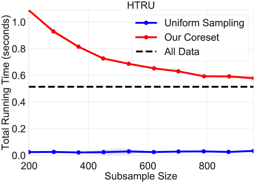
Refer to caption
Refer to caption
Refer to caption
Refer to caption
Refer to caption
Refer to caption
Figure 5: The total computational cost of constructing a coreset using the merge-and-reduce tree and training the SVM model the coreset, plotted as a function of the size of the coreset.