Monotonic Cardinality Estimation of Similarity Selection: A Deep Learning Approach

Yaoshu Wang Shenzhen Institute of Computing Sciences, Shenzhen University yaoshuw@sics.ac.cn , Chuan Xiao Osaka University
& Nagoya University chuanx@ist.osaka-u.ac.jp , Jianbin Qin Shenzhen Institute of Computing Sciences, Shenzhen University jqin@sics.ac.cn , Xin Cao The University of New South Wales xin.cao@unsw.edu.au , Yifang Sun The University of New South Wales yifangs@cse.unsw.edu.au , Wei Wang The University of New South Wales weiw@cse.unsw.edu.au and Makoto Onizuka Osaka University onizuka@ist.osaka-u.ac.jp

Abstract.

Due to the outstanding capability of capturing underlying data distributions, deep learning techniques have been recently utilized for a series of traditional database problems. In this paper, we investigate the possibilities of utilizing deep learning for cardinality estimation of similarity selection. Answering this problem accurately and efficiently is essential to many data management applications, especially for query optimization. Moreover, in some applications the estimated cardinality is supposed to be consistent and interpretable. Hence a monotonic estimation w.r.t. the query threshold is preferred. We propose a novel and generic method that can be applied to any data type and distance function. Our method consists of a feature extraction model and a regression model. The feature extraction model transforms original data and threshold to a Hamming space, in which a deep learning-based regression model is utilized to exploit the incremental property of cardinality w.r.t. the threshold for both accuracy and monotonicity. We develop a training strategy tailored to our model as well as techniques for fast estimation. We also discuss how to handle updates. We demonstrate the accuracy and the efficiency of our method through experiments, and show how it improves the performance of a query optimizer.

cardinality estimation; similarity selection; machine learning for data management

^†^†copyright: rightsretained^†^†conference: ; ; ^†^†ccs: Information systems Query optimization^†^†ccs: Computing methodologies Neural networks^†^†ccs: Information systems Entity resolution

1. Introduction

Deep learning has been recently utilized to deal with traditional database problems, such as indexing (kraska2018case, ), query execution (kraska2019sagedb, ; DBLP:conf/sigmod/DingDM0CN19, ; treedeepmodel, ; surveycarddeeplearning, ), and database tuning (DBLP:conf/sigmod/ZhangLZLXCXWCLR19, ). Compared to traditional database methods and non-deep-learning models (logistic regression, random forest, etc.), deep learning exhibits outstanding capability of reflecting the underlying patterns and correlations of data as well as exceptions and outliers that capture the extreme anomalies of data instances (kraska2019sagedb, ).

In this paper, we explore in the direction of applying deep learning techniques for a data management problem – cardinality estimation of similarity selection, i.e., given a set of records $\mathcal{D}$ , a query record $x$ , a distance function and a threshold $\theta$ , to estimate the number of records in $\mathcal{D}$ whose distances to $x$ are no greater than $\theta$ . It is an essential procedure in many data management tasks, such as search and retrieval, data integration, data exploration, and query optimization. For example: (1) In image retrieval, images are converted to binary vectors (e.g., by a HashNet (cao2017hashnet, )), and then the vectors whose Hamming distances to the query are within a threshold of 16 are identified as candidates (DBLP:conf/mm/ZhangGZL11, ) for further image-level verification (e.g, by a CNN). Since the image-level verification is costly, estimating the cardinalities of similarity selection yields the number of candidates, and thus helps estimate the overall running time in an end-to-end system to create a service level agreement. (2) In query optimization, estimating cardinalities for similarity selection benefits the computation of operation costs and the choice of execution orders of query plans that involve multiple similarity predicates; e.g., hands-off entity matching systems (DBLP:conf/sigmod/GokhaleDDNRSZ14, ; DBLP:conf/sigmod/DasCDNKDARP17, ) extract paths from random forests and take each path (a conjunction of similarity predicates over multiple attributes) as a blocking rule. Such query was also studied in (DBLP:conf/sigmod/LiHDL15, ) for sets and strings.

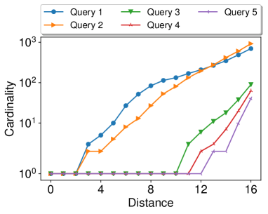
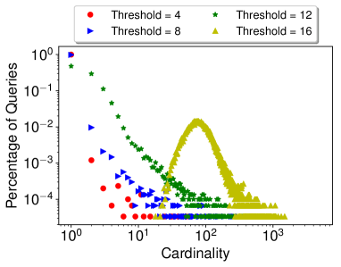
Refer to caption — (a) Cardinality v.s. threshold.

The reason why deep learning approaches may outperform other options for cardinality estimation of similarity selection can be seen from the following example: (1) Figure 1(a) shows the cardinalities of five randomly chosen queries on the ImageNet dataset (URL:imagenet, ) by varying Hamming distance threshold. The cardinalities keep unchanged at some thresholds but surge at others. (2) Figure 1(b) shows the percentage of queries (out of 30,000) for each cardinality value, under Hamming distance thresholds 4, 8, 12, and 16. The cardinalities are small or moderate for most queries, yet exceptionally large for long-tail queries (on the right side of the figure). Both facts cause considerable difficulties for traditional database methods which require large samples to achieve good accuracy and traditional learning methods which are incapable to learn such complex underlying distributions. In contrast, deep learning is a good candidate to capture such data patterns and generalizes well on queries that are not covered by training data, thereby delivering better accuracy. Another reason for choosing deep learning is that the training data – though large training sets are usually needed for deep learning – are easily acquired by running similarity selection algorithms (without producing label noise when exact algorithms are used).

In addition to accuracy, there are several other technical issues for cardinality estimation of similarity selection: (1) A good estimation is supposed to be fast. (2) A generic method that applies to a variety of data types and distance functions is preferred. (3) Users may want the estimated cardinality to be consistent and interpretable in applications like data exploration. Since the actual cardinality is monotonically increasing with the threshold, when a greater threshold is given, a larger or equal number of results is preferable, so the user is able to interpret the cardinality for better analysis.

To cope with these technical issues, we propose a novel method that separates data modelling and cardinality estimation into two components:

•

A feature extraction component transforms original data and thresholds to a Hamming space such that the semantics of the input distance function is exactly or approximately captured by Hamming distance. As such, our method becomes generic and applies to any data type and distance.
•

A regression component models the estimation as a regression problem and estimates the cardinality on the transformed vectors and threshold using deep learning.

To achieve good accuracy of regression, rather than feeding a deep neural network with training data in a straightforward manner, we devise a novel approach based on incremental prediction to exploit the incremental property of cardinality; i.e., when the threshold is increasing, the increment of cardinality is only caused by the records in the increased range of distance. Since our feature extraction maps original distances to discrete distance values, we can use multiple regressors, each dealing with one distance value, and then sum up the individual results to get the total cardinality. In doing so, we are able to learn the cardinality distribution for each distance value, so the overall estimation becomes more accurate. Another benefit of incremental prediction is that it guarantees the monotonicity w.r.t. the threshold, and thus yields more interpretability of the estimated results. To estimate the cardinality of each distance value, we utilize an encoder-decoder model through careful neural network design: (1) To cope with the sparsity in Hamming space, as output by the feature extraction, we employ a variational auto-encoder to embed the binary vector in Hamming space to a dense representation. (2) To generalize for queries and thresholds not covered by the training data, we also embed (Hamming) distance values. The distance embeddings are concatenated to the binary vector and its dense representation, and then fed to a neural network to produce final embeddings. The decoders takes the final embeddings as input and outputs the estimated cardinality.

We design a loss function and a dynamic training strategy, both tailored to our incremental prediction model. The loss function adds more loss to the distance values that tend to cause more estimation error. The impact of such loss is dynamically adjusted through training to improve the accuracy and the generalizability. For fast online estimation, optimizations are developed on top of our regression model by reducing multiple encoders to one. As we are applying machine learning on a traditional database problem, an important issue is whether the solution works when update exists. For this reason, we discuss incremental learning to handle updates in the dataset.

Extensive experiments were carried out on four common distance functions using real datasets. We took a uniform sample of records from each dataset as a query workload for training, validation, and testing, and computed labels by running exact similarity selection algorithms. The takeaways are: (1) The proposed deep learning method is more accurate than existing methods while also running faster with a moderate model size. (2) Incremental prediction guarantees monotonicity and at the same time achieves high accuracy, substantially outperforming the method that simply feeding a deep neural network with training data. (3) The components in our model are all useful to improve accuracy and speed. (4) Incremental learning is fast and effective against updates. (5) Our method delivers excellent performance on long-tail queries having exceptionally large cardinalities and generalizes well on out-of-dataset queries that significantly differ from the dataset. (6) A case study shows that query processing performance is improved by integrating our method into a query optimizer.

Our contributions are summarized as follows.

•

We develop a deep learning method for cardinality estimation of similarity selection (Section 3). Our method guarantees the monotonicity of cardinality w.r.t. the threshold.
•

Through feature extraction (Section 4) and regression (Section 5), our method is generic to any data type and distance function, and exploits the incremental property of cardinality to achieve accuracy and monotonicity. The training techniques that favor our method are developed (Section 6).
•

We accelerate our model for online estimation (Section 7) and propose incremental learning for updates (Section 8).
•

We conduct extensive experiments to demonstrate the superiority and the generalizability of our method, as well as how it works in a query optimizer (Section 9).

2. Preliminaries

2.1. Problem Definition and Notations

Let $\mathcal{O}$ be a universe of records. $x$ and $y$ are two records in $\mathcal{O}$ . $f:\mathcal{O}\times\mathcal{O}\to\mathbb{R}$ is a function which evaluates the distance (similarity) of a pair of records. Common distance (similarity) functions include Hamming distance, Jaccard similarity, edit distance, Euclidean distance, etc. Without loss of generality, we assume $f$ is distance function. Given a collection of records $\mathcal{D}\subseteq\mathcal{O}$ , a query record $x\in\mathcal{O}$ , and a threshold $\theta$ , a similarity selection is to find all the records $y\in\mathcal{D}$ such that $f(x,y)\leq\theta$ . We formally define our problem.

Problem 1 (Cardinality Estimation of Similarity Selection).

Given a collection $\mathcal{D}$ of records, a query record $x\in\mathcal{O}$ , a distance function $f$ , and a threshold $\theta\in[0,\theta_{\max}]$ , our task is to estimate the number of records that satisfy the similarity constraint, i.e., $|\{\,y\mid f(x,y)\leq\theta,y\in\mathcal{D}\,\}|$ .

$\theta_{\max}$ is the maximum threshold (reasonably large for similarity selection to make sense) we are going to support. A good estimation is supposed to be close to the actual cardinality. Mean squared error (MSE) and mean absolute percentage error (MAPE) are two widely used evaluation metrics in the cardinality estimation problem (DBLP:conf/sigmod/DasguptaJJZD10, ; wu2018local, ; DBLP:conf/edbt/MattigFBS18, ; DBLP:conf/sigmod/HeimelKM15, ; liu2015cardinality, ). Given $n$ similarity selection queries, let $c_{i}$ denote the actual cardinality of the $i$ -th selection and $\widehat{c}_{i}$ denote the estimated cardinality. MSE and MAPE are computed as

\displaystyle\textsf{MSE}=\frac{1}{n}\sum_{i=1}^{n}(c_{i}-\widehat{c}_{i})^{2},\quad\textsf{MAPE}=\frac{1}{n}\sum_{i=1}^{n}\left|{\frac{c_{i}-\widehat{c}_{i}}{c_{i}}}\right|.

Smaller errors are preferred. We adopt these two metrics to evaluate the estimation accuracy. We focus on evaluating the cardinality estimation as stand-alone (in contrast to in an RDBMS) and only consider in-memory implementations.

Table 1 lists the notations frequently used in this paper. We use bold uppercase letters (e.g., $\mathbf{A}$ ) for matrices; bold lowercase letters (e.g., $\mathbf{a}$ ) for vectors; and non-bold lowercase letters (e.g., $a$ ) for scalars and other variables. Uppercase Greek symbols (e.g., $\Phi$ ) are used to denote neural networks. $\mathbf{A}[i,*]$ and $\mathbf{A}[*,i]$ denote the $i$ -th row and the $i$ -th column of $\mathbf{A}$ , respectively. $\mathbf{a}[i]$ denotes the $i$ -th dimension of $\mathbf{a}$ . Semicolon represents the concatenation of vectors; e.g., given an $a$ -dimensional vector $\mathbf{a}$ and a $b$ -dimensional vector $\mathbf{b}$ , $\mathbf{c}=[\mathbf{a};\mathbf{b}]$ means that $\mathbf{c}[1\,\ldotp\ldotp\,a]=\mathbf{a}$ and $\mathbf{c}[a+1\,\ldotp\ldotp\,a+b]=\mathbf{b}$ . Colon represents the construction of a matrix by column vectors or matrices; e.g., $\mathbf{C}=[\mathbf{a}:\mathbf{b}]$ means that $\mathbf{C}[*,1]=\mathbf{a}$ and $\mathbf{C}[*,2]=\mathbf{b}$ .

Table 1. Frequently used notations.

Symbol	Definition
$\mathcal{O}$ , $\mathcal{D}$	a record universe, a dataset
$x,y$	records in $\mathcal{O}$
$f$	a distance function
$\theta$ , $\theta_{\max}$	a distance threshold and its maximum value
$c$ , $\widehat{c}$	cardinality and the estimated value
$g$ , $h$	regression function and feature extraction function
$\mathbf{x}$ , $d$	the binary representation of $x$ and its dimensionality
$\tau$ , $\tau_{\max}$	a threshold in Hamming space and its maximum value
$\mathbf{e}^{i}$	the embedding of distance $i$
$\mathbf{z}_{x}^{i}$	the embedding of $\mathbf{x}$ and distance $i$

2.2. Related Work

2.2.1. Database Methods

Auxiliary data structure is one of the main types of database methods for the cardinality estimation of similarity selection. For binary vectors, histograms (qin2018gph, ) can be constructed to count the number of records by partitioning dimensions into buckets and enumerating binary vectors and thresholds. For strings and sets, semi-lattice structures (lee2007extending, ; lee2009power, ) and inverted indexes (jin2008sepia, ; mazeika2007estimating, ) are utilized for estimation. The major drawback of auxiliary structure methods is that they only perform well on low dimensionality and small thresholds. Another type of database methods is based on sampling, e.g., uniform sampling, adaptive sampling (lipton1990query, ), and sequential sampling (haas1992sequential, ). State-of-the-art sampling strategies (wu2016sampling, ; DBLP:conf/sigmod/ZhaoC0HY18, ; DBLP:conf/icml/Jiang17a, ; leis2017cardinality, ) focus on join size estimation in query optimization, and are difficult to be adopted to our problem defined on distance functions. Sampling methods are often combined with sketches (DBLP:conf/vldb/GionisIM99, ; lee2011similarity, ) to improve the performance. A state-of-the-art method was proposed in (wu2018local, ) for high-dimensional data. In general, sampling methods need a large set of samples to achieve good accuracy, and thus become either slow or inaccurate when applied on large datasets. As for the cardinalities of SQL queries, recent studies proposed a tighter bound for intermediate join cardinalities (pesscardinality, ) and adopted inaccurate cardinalities to generate optimal query plans (cardqueryopt, ).

2.2.2. Traditional Learning Models

A prevalent traditional learning method for the cardinality estimation of similarity selection is to train a kernel-based estimator (DBLP:conf/sigmod/HeimelKM15, ; DBLP:conf/edbt/MattigFBS18, ) using a sample. Monotonicity is guaranteed when the sample is deterministic w.r.t. the query record (i.e., the sample does not change if only the threshold changes). Kernel methods require large number of instances for accurate estimation, hence resulting in low estimation speed. Moreover, they impose strong assumptions on kernel functions, e.g., only diagonal covariance matrix for Gaussian kernels. Other traditional learning models (ivanov2017adaptive, ), such as support vector regression, logistic regression, and gradient boosting tree, are also adopted to solve the cardinality estimation problem. A query-driven approach (anagnostopoulos2017query, ) was proposed to learn several query prototypes (i.e., interpolation) that are differentiable. These approaches deliver comparable performance to kernel methods. A recent study (DBLP:journals/pvldb/DuttWNKNC19, ) explored the application of two-hidden-layer neural networks and tree-based ensembles (random forest and gradient boosted trees) on cardinality estimation of multi-dimensional range queries. It targets numerical attributes but does not apply to similarity selections.

2.2.3. Deep Learning Models

Deep learning models are recently adopted to learn the best join order (krishnan2018learning, ; marcus2018deep, ; neoqueryoptimizer, ) or estimate the join size (kipf2018learned, ). Deep reinforcement learning is also explored to generate query plans (ortiz2018learning, ). Recent studies also adopted local-oriented approach (cardlocaldeepmodel, ), tree or plan based learning model (treedeepmodel, ; plandeeppredict, ; neoqueryoptimizer, ), recurrent neural network (surveycarddeeplearning, ), and autoregressive model (autogressivemultiattr, ; autoregressivelikelihood, ). The method that can be adapted to solve our problem is the mixture of expert model (shazeer2017outrageously, ). It utilizes a sparsely-gated mixture-of-experts layer and assigns good experts (models) to these inputs. Based on this model, the recursive-model index (kraska2018case, ) was designed to replace the traditional B-tree index for range queries. The two models deliver good accuracy but do not guarantee monotonicity.

For monotonic methods, an early attempt used a min-max 4-layer neural network for regression (daniels2010monotone, ). Lattice regression (garcia2009lattice, ; gupta2016monotonic, ; fard2016fast, ; you2017deep, ) is recent monotonic method. It adopts a lattice structure to construct all combinations of monotonic interpolation values. To handle high-dimensional monotonic features, ensemble of lattices (fard2016fast, ) splits lattices into several small pieces using ensemble learning. To improve the performance of regression, deep lattice network (DLN) was proposed (you2017deep, ). It consists of multiple calibration layers and an ensemble of lattices layers. However, lattice regression does not directly target our problem, and our experiments show that DLN is rather inaccurate.

3. Cardinality Estimation Framework

3.1. Basic Idea

Let $c(x,\theta)$ denote the cardinality of a query $x$ with threshold $\theta$ . We model the estimation as a regression problem with a unique framework designed to alleviate the challenges mentioned in Section 1. We would like to find a function $\widehat{c}$ within a function family, such that $\widehat{c}$ returns an approximate value of $c$ for any input $x$ , i.e., $\widehat{c}(x,\theta)\approx c(x,\theta),\forall x\in\mathcal{O}$ and $\theta\in[0,\theta_{\max}]$ . We consider $\widehat{c}$ that belongs to the following family: $\widehat{c}\coloneqq g\circ h$ , where $h(x,\theta)=(\mathbf{x},\tau)$ , $g(\mathbf{x},\tau)\in\mathbb{Z}_{\geq 0}$ , $\mathbf{x}\in\{\,0,1\,\}^{d}$ , and $\tau\in\mathbb{Z}_{\geq 0}$ . Intuitively, we can deem $h$ as a feature extraction function, which maps an object $x$ and a threshold $\theta$ to a fixed-dimensional binary vector $\mathbf{x}$ and an integer threshold $\tau$ . Then, the function $g$ essentially performs the regression using the transformed input, i.e., the $(\mathbf{x},\tau)$ pair. The rationales of such design are analyzed as follows:

•

This design separates data modelling and cardinality estimation into two functions, $h$ and $g$ , respectively. On one hand, this allows the system to cater for different data types, and distance functions. On the other hand, it allows us to choose the best models for the estimation problem. To decouple the two components, some common interface needs to be established. We pose the constraints that (1) $\mathbf{x}$ belonging to a Hamming space, and (2) $\tau$ is an non-negative integer. For (1), many DB applications deal with discrete objects (e.g., sets and strings) or discrete object representations (e.g., binary codes from learned hash functions). For (2), since there is a finite number of thresholds that make a difference in cardinality, in theory we can always map them to integers, albeit a large number. Here, we take the approximation to limit it to a fixed number. Other learning models also make similar modelling choice (e.g., most regularizations adopt the smoothness bias in the function space). We will leave other interface design choices to future work due to their added complexity. For instance, it is entirely possible to restrict $\mathbf{x}$ to $\mathbb{R}^{d}$ and $\tau\in\mathbb{R}$ . While the modelling power of the framework gets increased, this will inevitably result in more complex models that are potentially difficult to train.
•

The design can be deemed as an instance of the encoder-decoder model, where two functions $h$ and $g$ are used for some prediction tasks. As a close analog, Google translation (johnson2017google, ) trains an $h$ that maps inputs in the source language to a latent representation, and then train a $g$ that maps the latent representation to the destination language. As such, it can support translation between $n$ languages by training only $2n$ functions, instead of $n(n-1)$ direct functions.

By this model design, the function $\widehat{c}=g\circ h(x,\theta)$ is monotonic if it satisfies the condition in the following lemma.

Lemma 0.

Consider a function $h(x,\theta)$ monotonically increasing with $\theta$ and a function $g(\mathbf{x},\tau)$ monotonically increasing with $\tau$ , our framework $g\circ h(x,\theta)$ is monotonically increasing with $\theta$ .

3.2. Feature Extraction

The process of feature extraction is to transfer any data type and distance threshold into binary representation and integer threshold. Formally, we have a function $h_{rec}:\mathcal{O}\to\{\,0,1\,\}^{d}$ ; i.e., given any record $x\in\mathcal{O}$ , $h_{rec}$ maps $x$ to a $d$ -dimensional binary vector, denoted by $\mathbf{x}$ , called $x$ ’s binary representation. We can plug in any user-defined functions or neural networks for feature extraction. For the sake of estimation accuracy, the general criteria is that the Hamming distance of the target $d$ -dimensional binary vectors can equivalently or approximately capture the semantics of the original distance function. We will show some example feature extraction methods and a series of case studies in Section 4.

Besides the transformation to binary representations, we also have a monotonically increasing (as demanded by Lemma 1) function $h_{thr}:[0,\theta_{\max}]\to[0,\tau_{\max}]$ to transform the threshold. $\tau_{\max}$ is a tunable parameter to control the model size (as introduced later, there are $(\tau+1)$ decoders in our model, $\tau\leq\tau_{\max}$ ). Given a $\theta\in[0,\theta_{\max}]$ , $h_{thr}$ maps $\theta$ to an integer between $0$ and $\tau_{\max}$ , denoted by $\tau$ . The purpose of threshold transformation is: for real-valued distance functions, it makes the distances countable; for integer-valued distance functions, it can reduce the threshold to a small number, hence to prevent the model growing too big when the input threshold is large. As such, we are able to use finite number of estimators to predict the cardinality for each distance value. The design of threshold transformation depends on how original data are transformed to binary representations. In general, a transformation with less skew leads to better performance. Using the threshold of the Hamming distance between binary representations is not necessary, but would be a preferable option. A few case studies will be given in Section 4.

3.3. Regression (in a Nutshell)

Our method for the regression is based on the following observation: given a binary representation $\mathbf{x}$ and a threshold $\tau$ ¹¹1Note that the threshold is $\tau$ not $\tau_{\max}$ here because $\theta$ is mapped to $\tau$ ., the cardinality can be divided into $(\tau+1)$ parts, each representing the cardinality of a Hamming distance $i$ , $i\in[0,\tau]$ . This suggests that we can learn $(\tau+1)$ functions $g_{0}(\mathbf{x}),\ldots,g_{\tau}(\mathbf{x})$ , each $g_{i}(\mathbf{x})$ estimating the cardinality of the set of records whose Hamming distances to $\mathbf{x}$ are exactly $i$ . So we have

(1)

\displaystyle g(\mathbf{x},\tau)=\sum_{i=0}^{\tau}{g_{i}(\mathbf{x})}.

This design has the following advantages:

•

As we have shown in Figure 1(a), the cardinalities for different distance values may differ significantly. By using individual estimators, the distribution of each distance value can be learned separately to achieve better overall accuracy.
•

Our method exploits the incremental property of cardinality: when the threshold increases from $i$ to $i+1$ , the increased cardinality is the cardinality for distance $i+1$ . This incremental prediction can guarantee the monotonicity of cardinality estimation:

Lemma 0.

$g(\mathbf{x},\tau)$ is monotonically increasing with $\tau$ , if each $g_{i}(\mathbf{x})$ , $i\in[0,\tau]$ is deterministic and non-negative.

The lemma suggests that a deterministic and non-negative model satisfies the requirement in Lemma 1, hence leading to the overall monotonicity.
•

We are able to control the size of the model by setting the maximum number of estimators. Thus, working with the feature extraction, the regression achieves fast speed even if the original threshold is large.

We employ a deep encoder-decoder model to process each regression $g_{i}$ . The reasons for choosing deep models are: (1) Cardinalities may significantly differ across queries, as shown in Figure 1(b). Deep models are able to learn a variety of underlying distributions and deliver salient performance for general regression tasks (shazeer2017outrageously, ; kraska2018case, ; you2017deep, ). (2) Deep models generalize well on queries that are not covered by the training data. (3) Although deep models usually need large training sets for good accuracy, the training data here can be easily and efficiently acquired by running state-of-the-art similarity selection algorithms (and producing no label noise when exact algorithms are used). (4) Deep models can be accelerated by modern hardware (e.g., GPUs/TPUs) or software (e.g., Tensorflow) that optimizes batch strategies or matrix manipulation ²²2Despite such possibilities for acceleration, we only use them for training but not inference (estimation) in our experiments for the sake of fair comparison..

We employ a deep learning model to process each regression $g_{i}$ . By carefully choosing encoders and decoders, we can meet the requirement in Lemma 2 to guarantee the monotonicity. The details will be given in Section 5. Before that, we show some options and case studies of feature extraction.

4. Case Studies for Feature Extraction

As stated in Section 3.2, for good accuracy, a desirable feature extraction is that the Hamming distance between the binary vectors can capture the semantics of the original distance function. We discuss a few example options.

•

Equivalency: Some distances can be equivalently expressed in a Hamming space, e.g., $L_{1}$ distance on integer values (DBLP:conf/vldb/GionisIM99, ).
•

LSH: We use $d$ hash functions in the locality sensitive hashing (LSH) family (DBLP:conf/vldb/GionisIM99, ), each hashing a record to a bit. $\mathbf{x}$ and $\mathbf{y}$ agree on a bit with high probability if $f(x,y)\leq\theta$ , thus yielding a small Hamming distance between $\mathbf{x}$ and $\mathbf{y}$ .
•

Bounding: We may derive a necessary condition of the original distance constraint; e.g., $f(x,y)\leq\theta\implies H(\mathbf{x},\mathbf{y})\leq\tau$ , where $H(\cdot,\cdot)$ denotes the Hamming distance.

For the equivalency method, since the conversion to Hamming distance is lossless, it can be used atop of the other two. This is useful when the output of the hash function or the bound is not in a Hamming space. Note that our model is not limited to these options. Other feature extraction methods, such as embedding (DBLP:conf/kdd/Zhang017, ), can be also used here.

As for threshold transformation, we have two parameters: $\theta_{\max}$ , the maximum threshold we are going to support, and $\tau_{\max}$ , a tunable parameter to control the size of our model. Any threshold $\theta\in[0,\theta_{\max}]$ is monotonically mapped to an integer $\tau\in[0,\tau_{\max}]$ . In our case studies, we consider using a transformation proportional to the (expected/bounded) Hamming distance between binary representations. Note that $\theta_{\max}$ is not necessarily mapped to $\tau_{\max}$ , because for integer-valued distance functions, the number of available thresholds is smaller than $\tau_{\max}+1$ when $\theta_{\max}<\tau_{\max}$ , meaning that only $(\theta_{\max}+1)$ decoders are useful. In this case, $\theta_{\max}$ is mapped to a value smaller than $\tau_{\max}$ . Next we show four case studies of some common data types and distance functions.

4.1. Hamming Distance

We consider binary vector data and Hamming distance as the input distance function. The original data are directly fed to our regression model. Since the function is already Hamming distance, we use the original threshold $\theta$ as $\tau$ , if $\theta_{\max}\leq\tau_{\max}$ . Otherwise, we map $\theta_{\max}$ to $\tau_{\max}$ , and other thresholds are mapped proportionally: $\tau=\lfloor\tau_{\max}\cdot\theta/\theta_{\max}\rfloor$ . Although multiple thresholds may map to the same $\tau$ , we can increase the number of decoders to mitigate the imprecision.

4.2. Edit Distance

The (Levenshtein) edit distance measures the minimum number of operations, including insertion, deletion, and substitution of a character, to transform one string to another.

The feature extraction is based on bounding. The basic idea is to map each character to $(2\tau_{\max}+1)$ bits, hence to cover the effect of insertion and deletion. Let $\Sigma$ denote the alphabet of strings, and $l_{\max}$ denote the maximum string length in $\mathcal{D}$ . Each binary vector has $d=((l_{\max}+2\tau_{\max})\cdot|\Sigma|)$ bits. They are divided into $|\Sigma|$ groups, each group representing a character in $\Sigma$ . For ease of exposition, we assume the subscript of a string start from $0$ , and the subscript of each group of the binary vector start from $-\tau_{\max}$ . All the bits are initialized as $0$ . Given a string $x$ , for each character $\sigma$ at position $i$ , we set the $j$ -th bit in the $\sigma$ -th group to $1$ , where $j$ iterates through $i-\tau_{\max}$ to $i+\tau_{\max}$ . For example, given a string $x=\texttt{abc}$ , $\Sigma=\{\,\texttt{a},\texttt{b},\texttt{c},\texttt{d}\,\}$ , $l_{\max}=4$ , and $\tau_{max}=1$ , the binary vector is 111000, 011100, 001110, 000000 (groups separated by comma).

It can be proved that an edit operation causes at most $(4\tau_{\max}+2)$ different bits. Hence $f(x,y)$ edit operations yield a Hamming distance no greater than $f(x,y)\cdot(4\tau_{\max}+2)$ . Since it is proportional to $f(x,y)$ and thresholds are integers, we use the same threshold transformation as for Hamming distance.

4.3. Jaccard Distance

We use $b$ -bit minwise hashing (li2010b, ) (LSH) for feature extraction. Given a record $x$ , $\pi(x)$ orders the elements of $x$ by a permutation on the record universe $\mathcal{O}$ . We uniformly choose a set of $k$ permutations $\{\,\pi_{1},\ldots,\pi_{k}\,\}$ . Let $bmin(\pi(x))$ denote the last $b$ bits of the smallest element of $\pi(x)$ . We regard $bmin(\pi(x))$ as an integer in $[0,2^{b}-1]$ and transform it to a Hamming space. Let $set\_bit(i,j)$ produce a one-hot binary vector such that only the $i$ -th bit is $1$ out of $j$ bits. $x$ is transformed to a $d$ -dimensional ( $d=2^{b}k$ ) binary vector: $[set\_bit(bmin(\pi_{1}(x)),2^{b});\ldots;set\_bit(bmin(\pi_{k}(x)),2^{b})]$ . For example: $x=\{\,1,2,4\,\}$ . $\mathcal{O}=\{\,1,2,3,4,5\,\}$ . $\pi_{1}=12345$ , $\pi_{2}=54321$ , and $\pi_{3}=21453$ . $b=2$ . We have $bmin(\pi_{1}(x))=1$ , $bmin(\pi_{2}(x))=0$ , and $bmin(\pi_{3}(x))=2$ . Suppose $set\_bit$ counts from the lowest bit, starting from $0$ . The binary vector is 0010, 0001, 0100 (permutations separated by comma).

Given two sets $x$ and $y$ , the probability that $bmin(\pi(x))=bmin(\pi(y))$ equals to $1-f(x,y)$ (li2010b, ). The expected Hamming distance between $\mathbf{x}$ and $\mathbf{y}$ is thus $f(x,y)\cdot d$ . Since it is proportional to $f(x,y)$ , we use the following threshold transformation: $\tau=\lfloor\tau_{\max}\cdot\theta/\theta_{\max}\rfloor$ .

4.4. Euclidean Distance

We use LSH based on $p$ -stable distribution (datar2004locality, ) to handle Euclidean distance on real-valued vectors. The hash function is $h_{\mathbf{a},b}(x)=\lfloor\frac{\mathbf{a}x+b}{r}\rfloor$ , where $\mathbf{a}$ is a $|x|$ -dimensional vector with each element independently drawn by a normal distribution $\mathcal{N}(0,1)$ , $b$ is a real number chosen uniformly from $[0,r]$ , and $r$ is a predefined constant value. Let $v$ denote the maximum hash value. We use the aforementioned $set\_bit$ function to transform hash values to a Hamming space. Given $k$ hash functions, $x$ is transformed to a $d$ -dimensional ( $d=k(v+1)$ ) binary vector: $[set\_bit(h_{\mathbf{a}_{1},b_{1}}(x),v+1);\ldots;set\_bit(h_{\mathbf{a}_{k},b_{k}}(x),v+1)]$ . For example: $x=[0.1,0.2,0.4]$ . $v=4$ . $h_{\mathbf{a}_{1},b_{1}}(x)=1$ . $h_{\mathbf{a}_{2},b_{2}}(x)=3$ . $h_{\mathbf{a}_{3},b_{3}}(x)=4$ . Suppose $set\_bit$ counts from the lowest bit, starting from $0$ . The binary vector is 00010, 01000, 10000 (hash functions separated by comma).

Given two records $x$ and $y$ such that $f(x,y)=\theta$ , the probability that two hash values match is $Pr\{\,h_{\mathbf{a},b}(x)=h_{\mathbf{a},b}(y)\,\}=\epsilon(\theta)$ $=1-2\cdot norm(-r/\theta)-\frac{2}{\sqrt{2\pi}r/\theta}(1-e^{-(r^{2}/2\theta^{2})})$ , where $norm(\cdot)$ is the cumulative distribution function of a random variable with normal distribution $\mathcal{N}(0,1)$ (datar2004locality, ). Hence the expected Hamming distance between their binary representations is $(1-\epsilon(\theta))\cdot d$ . The threshold transformation is $\tau=\lfloor\tau_{\max}\cdot\frac{1-\epsilon(\theta)}{1-\epsilon(\theta_{\max})}\rfloor$ .

5. Regression

We present the detailed regression model in this section. Figure 2 shows the framework of our model. (1) $\mathbf{x}$ and $\tau$ are input to the encoder $\Psi$ , which returns $\tau+1$ embeddings $\mathbf{z}_{x}^{i}$ . Specifically, $\mathbf{x}$ is embedded to a dense vector space. Each distance $i$ is also embedded, concatenated to the embedding of $\mathbf{x}$ , and fed to a neural network $\Phi$ to produce $\mathbf{z}_{x}^{i}$ . (2) Each of the $\tau+1$ decoders $g_{i}$ takes an embedding $\mathbf{z}_{x}^{i}$ as input and returns the cardinality of distance $i$ , $i\in[0,\tau]$ . (3) The $\tau+1$ cardinalities are summed up to get the final cardinality.

5.1. Encoder-Decoder Model

Our solution to the regression is to embed the binary vector $\mathbf{x}$ and distance $i$ to a dense real-valued vector $\mathbf{z}^{1}_{x}$ by an encoder $\Psi$ , and then model $g_{i}(\mathbf{x})$ as a decoder that performs an affine transformation and applies an ReLU activation function:

\displaystyle g_{i}(\mathbf{x})=\textsf{ReLU}(\mathbf{w}_{i}^{\rm T}\Psi(\mathbf{x},i)+b_{i})=\textsf{ReLU}(\mathbf{w}_{i}^{\rm T}\mathbf{z}^{i}_{x}+b_{i}).

$\mathbf{w}_{i}$ and $b_{i}$ are parameters of the mapping from the embedding $\mathbf{z}^{i}_{x}$ to the cardinality estimation of distance $i$ . From the machine learning perspective, if a representation of input features is well learned through an encoder, then a linear model (affine transformation) is capable of making final decisions (bengio2013representation, ). ReLU is chosen here because cardinality is non-negative and matches the range of ReLU. The reason why we also embed distance $i$ is as follows. Consider only $\mathbf{x}$ is embedded. If the cardinalities of two records $x_{1}$ and $x_{2}$ are close for distance values in a range $[\tau_{1},\tau_{2}]$ covered by the training examples, their embeddings are likely to become similar after training, because the encoder may mistakenly regard $x_{1}$ and $x_{2}$ as similar. This may cause $g_{i}(\mathbf{x}_{1})\approx g_{i}(\mathbf{x}_{2})$ for $i\notin[\tau_{1},\tau_{2}]$ , i.e., the distance values not covered by the training examples, even if their actual cardinalities significantly differ.

By Equation 1, the output of the $\tau$ decoders are summed up to obtain the cardinality. $g_{i}(\mathbf{x})$ is deterministic if we use a deterministic $\Psi(\cdot,\cdot)$ . Hence the model can satisfy the requirement in Lemma 2 to guarantee the monotonicity.

5.2. Encoder in Detail

To encode both $\mathbf{x}$ and distance $i$ to embedding $\mathbf{z}^{i}_{x}$ , $\Psi$ includes a representation network $\Gamma$ that maps $\mathbf{x}$ to a dense vector space, a distance embedding layer $\mathbf{E}$ , and a shared neural network $\Phi$ that outputs the embedding $\mathbf{z}^{i}_{x}$ . Next we introduce the details.

5.2.1. Representation Network

Given a binary representation $\mathbf{x}$ generated by feature extraction function $h(\cdot,\cdot)$ , we design a neural network $\Gamma$ that maps $\mathbf{x}$ to another vector space: $\mathbf{x}^{\prime}=\Gamma(\mathbf{x})$ , because the correlations of sparse high-dimensional binary vectors are difficult to learn. Variational auto-encoder (VAE) (kingma2013auto, ) is a generative model to estimate data distribution by unsupervised learning. We can view auto-encoders (AEs) as non-linear PCAs to reduce dimensionality and extract meaningful and robust features, and VAE enforces continuity in the latent space. VAE improves upon other types of AEs (such as denoising AEs and sparse AEs) by imposing some regularization condition on the embeddings. This results in embeddings that are robust and disentangled, and hence have been widely used in various models (DBLP:journals/corr/abs-1812-05069, ). We use the latent layer of VAE to produce a dense representation, denoted by $VAE(\mathbf{x},\epsilon)$ . $\epsilon$ is a random noise generated by normal distribution $\mathcal{N}(0,\mathbf{I})$ . $\Gamma$ concatenates $\mathbf{x}$ and the output of VAE; i.e., $\mathbf{x}^{\prime}=[\mathbf{x};VAE(\mathbf{x},\epsilon)]$ . The reason for such concatenation (i.e., not using only the output of VAE as $\mathbf{x}^{\prime}$ ) is that the (cosine) distance in the $VAE(\mathbf{x},\epsilon)$ space captures less semantics of the original distance than does the Hamming distance between binary vectors. Due to the noise $\epsilon$ , the output of VAE becomes nondeterministic. Since we need a deterministic output to guarantee the monotonicity, we choose the following option: for training, we still use the nondeterministic $\mathbf{x}^{\prime}=[\mathbf{x};VAE(\mathbf{x},\epsilon)]$ , because this makes our model generalize to unseen records and thresholds; for inference (online estimation), we set $\mathbf{x}^{\prime}=[\mathbf{x};\mathrm{E}_{\epsilon\sim\mathcal{N}(0,\mathbf{I})}[VAE(\mathbf{x},\epsilon)]]$ , where $\mathrm{E}[\cdot]$ denotes the expected value, so it becomes deterministic (sohn2015learning, ).

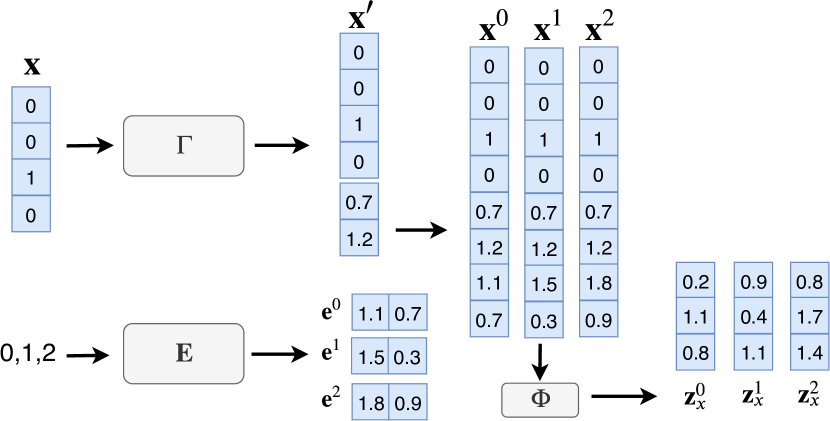
Example 0.

Figure 3 shows an example of $\mathbf{x}$ and its embedding $\mathbf{x}^{\prime}$ . Suppose $\mathbf{x}=\texttt{0010}$ . The VAE takes $\mathbf{x}$ as input and output a dense vector, say $[0.7,1.2]$ . Then they are concatenated to obtain $\mathbf{x}^{\prime}=[\texttt{0010},0.7,1.2]$ .

5.2.2. Distance Embeddings

In order to embed $\mathbf{x}$ and distance $i$ into the same vector, we design a distance embedding layer (a matrix) $\mathbf{E}$ to embed each distance $i$ . Each column in $\mathbf{E}$ represents a distance embedding; i.e., $\mathbf{e}^{i}=\mathbf{E}[*,i]$ . $\mathbf{E}$ is initialized randomly, following standard normal distribution.

5.2.3. Final Embeddings

The distance embedding $\mathbf{e}^{i}$ is concatenated with $\mathbf{x}^{\prime}$ ; i.e., $\mathbf{x}^{i}=[\mathbf{x}^{\prime};\mathbf{e}^{i}]$ . Then we use a feedforward neural network (FNN) $\Phi$ to generate embeddings $\mathbf{z}^{i}_{x}=\Phi(\mathbf{x}^{i})$ .

Example 0.

We follow Example 1. Suppose $\tau=2$ . Then we have three distance embeddings $\mathbf{e}^{0}=[1.1,0.7]$ , $\mathbf{e}^{1}=[1.5,0.3]$ , and $\mathbf{e}^{2}=[1.8,0.9]$ . By concatenating $\mathbf{x}^{\prime}$ and each $\mathbf{e}^{i}$ , $\mathbf{x}^{0}=[\texttt{0010},0.7,1.2,1.1,0.7]$ , $\mathbf{x}^{1}=[\texttt{0010},0.7,1.2,1.5,0.3]$ , and $\mathbf{x}^{2}=[\texttt{0010},0.7,1.2,1.8,0.9]$ . They are sent to neural network $\Phi$ , whose output is $\mathbf{z}^{0}_{x}=[0.2,1.1,0.8]$ , $\mathbf{z}^{1}_{x}=[0.9,0.4,1.1]$ , and $\mathbf{z}^{2}_{x}=[0.8,1.7,1.4]$ .

6. Model Training

6.1. Data Preparation

Consider a query workload $\mathcal{Q}$ of records (see Section 9.1.1 for the choice of $\mathcal{Q}$ in our experiments). We split data in $\mathcal{Q}$ for training, validation, and testing sets. Then we uniformly generate a set of thresholds in $[0,\theta_{\max}]$ , denoted by $S$ . For each record $x$ in the training set, we iterate through all the thresholds $\theta$ in $S$ and compute the cardinality $c$ w.r.t. $\mathcal{D}$ using an exact similarity selection algorithm. Then $\langle\,x,\theta,c\,\rangle$ is used as a training example. We uniformly choose thresholds in $S$ for validation and in $[0,\theta_{\max}]$ for testing.

6.2. Loss Function & Dynamic Training

The loss function is defined as follows.

(2)

\displaystyle\mathcal{L}(\widehat{\mathbf{c}},\mathbf{c})=\mathrm{E}_{\mathbf{\tau}\sim P(\cdot)}[\mathcal{L}_{g}(\widehat{\mathbf{c}},\mathbf{c})]+\lambda\mathcal{L}_{vae}(\mathbf{x}),

where $\mathcal{L}_{g}(\cdot,\cdot)$ is the loss of regression model, and $\mathcal{L}_{vae}(\cdot)$ is the loss of VAE. $\widehat{\mathbf{c}}$ and $\mathbf{c}$ are two vectors, each dimension representing the estimated and the real cardinalities of a set of training examples, respectively. $\lambda$ is a positive hyperparameter for the importance of VAE. A caveat is that although we uniformly sample thresholds in $[0,\theta_{\max}]$ for training data, it does not necessarily mean the threshold $\tau$ after feature extraction is uniformly distributed in $[0,\tau_{\max}]$ , e.g., for Euclidean distance (Section 4.4). To take this factor into account, we approximate the probability of $\tau$ using the empirical probability of thresholds after running feature extraction on the validation set; i.e., $P(\tau)\approx\frac{\sum_{\langle\,x,i,c\,\rangle\in\mathcal{T}^{valid}}\mathbf{1}_{h_{thr}(i)=\tau}}{|\mathcal{T}^{valid}|}$ , where $\mathcal{T}^{valid}$ is the validation set, and $\mathbf{1}$ is the indicator function.

For $\mathcal{L}_{g}$ , instead of using MSE or MAPE, we resort to the mean squared logarithmic error (MSLE) for the following reason: MSLE is an approximation of MAPE (park1998relative, ) and narrows down the large output space to a smaller one, thereby decreasing the learning difficulty.

Then we propose a training strategy for better accuracy. Given a set of training examples, let $\mathbf{c}_{0}$ , $\ldots$ , $\mathbf{c}_{\tau}$ and $\widehat{\mathbf{c}_{0}}$ , $\ldots$ , $\widehat{\mathbf{c}_{\tau}}$ denote the cardinalities and the estimated values for distance $0$ , $\ldots$ , $\tau$ in these training examples, respectively. As we have shown in Figure 1(a), the cardinalities may vary significantly for different distance values. Some of them may result in much worse estimations than others and compromise the overall performance. The training procedure should gradually focus on training these bad estimations. Thus, we consider the loss caused by the estimation for distance $i$ , combined with MSLE:

(3)

\displaystyle\mathcal{L}_{g}(\widehat{\mathbf{c}},\mathbf{c})=\textsf{MSLE}(\widehat{\mathbf{c}},\mathbf{c})+\lambda_{\Delta}\cdot\bigg{(}\sum_{i=0}^{\tau_{max}}{\omega_{i}\cdot\textsf{MSLE}(\widehat{\mathbf{c}_{i}}.\mathbf{c}_{i})}\bigg{)}.

Each $\omega_{i}$ is a hyperparameter automatically adjusted during the training procedure. Hence we call it dynamic training. It controls the loss of each estimation for distance $i$ . $\sum_{i=0}^{\tau_{max}}{\omega_{i}}=1$ . $\lambda_{\Delta}$ is a hyperparameters to control the impact of the losses of all the estimations for $i\in[0,\tau_{\max}]$ .

Due to the non-convexity of $\mathcal{L}_{g}$ , it is difficult to find the correct direction of gradient that reaches the global or a good local optimum. Nonetheless, we can adjust its direction by considering the loss trend of the estimation for distance $i$ , hence to encourage the model to generalize rather than to overfit the training data. Let $\ell_{i}(t)=\textsf{MSLE}(\widehat{\mathbf{c}_{i}},\mathbf{c}_{i})$ denote the loss of the estimation for distance $i$ in the $t$ -th iteration of validation. The loss trend $\Delta\ell_{i}(t)=\ell_{i}(t)-\ell_{i}(t-1)$ is calculated, and then after each validation we adjust $\omega_{i}$ by adding more gradients to where the loss occurs: (1) If $\Delta\ell_{i}(t)>0$ , $\omega_{i}=\frac{\Delta\ell_{i}(t)}{\sum_{i\in A}{\Delta\ell_{i}(t)},\,A=\{\,i\mid\Delta\ell_{i}(t)>0,0\leq i\leq\tau_{\max}\,\}}$ ; (2) otherwise, $\omega_{i}=0$ .

7. Accelerating Estimation

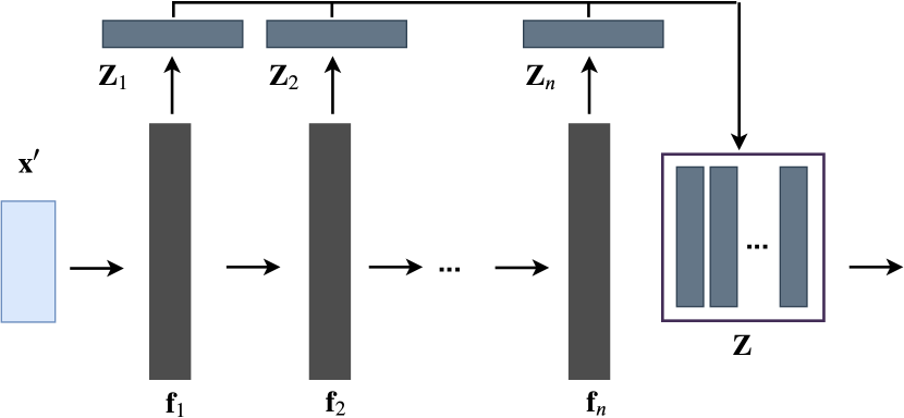
Recall in the regression model, we pair $\mathbf{x}^{\prime}$ and $(\tau+1)$ distance embeddings in encoder $\Psi$ to produce embedings $\mathbf{z}_{x}^{i}$ . This leads to high computation cost for online cardinality estimation when $\tau$ is large. To reduce the cost, we propose an accelerated model, using a neural network $\Phi^{\prime}$ to replace $\Phi$ and the distance embedding layer $\mathbf{E}$ to output $(\tau_{\max}+1)$ $\mathbf{z}_{x}^{i}$ embeddings together ³³3We output $(\tau_{\max}+1)$ embeddings since it is constant for all queries, hence to favor implementation. Only the first $(\tau+1)$ embedding are used for $\tau$ .. $\Phi^{\prime}$ only takes an input $\mathbf{x^{\prime}}$ and reduces the computation cost from $O((\tau+1)|\Phi|)$ to $O(|\Phi^{\prime}|)$ , where $|\Phi|$ and $|\Phi^{\prime}|$ denote the number of parameters in the two neural networks.

Figure 4 shows the framework of $\Phi^{\prime}$ , an FNN comprised of $n$ hidden layers $\mathbf{f}_{1}$ , $\mathbf{f}_{2}$ , $\ldots$ , $\mathbf{f}_{n}$ , each outputting some dimensions of the embeddings $\mathbf{z}_{x}^{i}$ . Each $\mathbf{z}^{i}_{x}$ is partitioned into $n$ regions, denoted by $\mathbf{z}^{i}_{x}[r_{0},r_{1}]$ , $\mathbf{z}^{i}_{x}[r_{1},r_{2}]$ , $\ldots$ , $\mathbf{z}^{i}_{x}[r_{n-1},r_{n}]$ , where $0=r_{0}\leq r_{1}\leq\ldots\leq r_{n}$ and $r_{n}$ equals to the dimensionality of $\mathbf{z}_{x}^{i}$ . A hidden layer $\mathbf{f}_{j}$ outputs the $j$ -th region of $\mathbf{z}_{x}^{i}$ , $i\in[0,\tau_{\max}]$ ; i.e., $\mathbf{Z}_{j}=[\mathbf{z}^{0}_{x}[r_{j-1},r_{j}]:\mathbf{z}^{1}_{x}[r_{j-1},r_{j}]:\ldots:\mathbf{z}^{\tau_{max}}_{x}[r_{j-1},r_{j}]]$ . Then we concatenate all the regions: $\mathbf{Z}=[\mathbf{Z}_{1}:\mathbf{Z}_{2}:\ldots:\mathbf{Z}_{n}]$ . Each row of $\mathbf{Z}$ is an embedding: $\mathbf{z}_{x}^{i}=\mathbf{Z}[i,*]$ .

In addition to fast estimation, the model $\Phi^{\prime}$ has the following advantages: (1) The parameters of each hidden layer $\mathbf{f}_{j}$ are updated from the following layer $\mathbf{f}_{j+1}$ and the final embedding matrix $\mathbf{Z}$ through backpropagation, hence increasing the ability to learn good embeddings. (2) Since each embedding is affected by all the hidden layers, the model is more likely to reach a better local optimum through training. (3) In contrast to one output layer, all the hidden layers output embeddings, so gradient vanishing and overfitting can be prevented.

We analyze the complexities of our models. Assume an FNN has hidden layers $\mathbf{a}_{1},\ldots,\mathbf{a}_{n}$ . Given an input $\mathbf{x}$ and an output $\mathbf{y}$ , the complexity of an FNN is $|\textsf{FNN}(\mathbf{x},\mathbf{y})|=|\mathbf{x}|\cdot|\mathbf{a}_{1}|+\sum_{i=1}^{n-1}{|\mathbf{a}_{i}|\cdot|\mathbf{a}_{i+1}|}+|\mathbf{a}_{n}|\cdot|\mathbf{y}|$ . Our model has the following components: $\Phi,\Gamma,\mathbf{E}$ , and $g_{i}$ . The complexities of $\Phi$ and $\Gamma$ are $|\textsf{FNN}([\mathbf{x}^{\prime};\mathbf{e}^{i}],\mathbf{z}_{x}^{i})|$ and $|\textsf{FNN}(\mathbf{x},\mathbf{x})|$ , respectively. $|\mathbf{E}|=(\tau_{\max}+1)|\mathbf{e}^{i}|$ . $|g_{i}|=(\tau_{\max}+1)|\mathbf{z}_{x}^{i}|+\tau_{\max}+1$ . Thus, the complexity of our model without acceleration is $|\textsf{FNN}([\mathbf{x}^{\prime};\mathbf{e}^{i}],\mathbf{z}_{x}^{i})|+|\textsf{FNN}(\mathbf{x},\mathbf{x})|+(\tau_{\max}+1)|\mathbf{e}^{i}|+(\tau_{\max}+1)|\mathbf{z}_{x}^{i}|+\tau_{\max}+1$ . With acceleration for FNN (AFNN), the complexity is $|\textsf{AFNN}(\mathbf{x}^{\prime},\mathbf{Z})|+|\textsf{FNN}(\mathbf{x},\mathbf{x})|+(\tau_{\max}+1)|\mathbf{z}_{x}^{i}|+\tau_{\max}+1$ , where $|\textsf{AFNN}(\mathbf{x}^{\prime},\mathbf{Z})|=|\mathbf{x}^{\prime}|\cdot|\mathbf{a}_{1}|+\sum_{i=1}^{n-1}{|\mathbf{a}_{i}|\cdot|\mathbf{a}_{i+1}|}+(\tau_{\max}+1)|\mathbf{a}_{n}|\cdot|\mathbf{Z}[i,*]|$ .

8. Dealing with Updates

When the dataset is updated, the labels of the validation data are first updated by running a similarity selection algorithm on the updated dataset. Then we monitor the error (MSLE) in the validated data by running our model. If the error increases, we train our model with incremental learning: First, the labels of the training data are updated by running a similarity selection algorithm on the updated dataset. Then the model is trained with the updated training data until the validation error does not change for three consecutive epochs. Note that (1) the training does not start from scratch but from the current model, and it is processed on the entire training data to prevent catastrophic forgetting (mccloskey1989catastrophic, ; kemker2018measuring, ); and (2) we always keep the original queries and only update their labels.

Table 2. Statistics of datasets.

Dataset	Source	Process	Data Type	Domain	# Records	$\ell_{max}$	$\ell_{avg}$	Distance	$\theta_{max}$
HM-ImageNet	(URL:imagenet, )	HashNet (cao2017hashnet, )	binary vector	image	1,431,167	64	64	Hamming	20
HM-PubChem	(URL:pubchem, )	-	binary vector	biological sequence	1,000,000	881	881	Hamming	30
ED-AMiner	(URL:aminer, )	-	string	author name	1,712,433	109	13.02	edit	10
ED-DBLP	(URL:dblp, )	-	string	publication title	1,000,000	199	72.49	edit	20
JC-BMS	(URL:bms-pos, )	-	set	product entry	515,597	164	6.54	Jaccard	0.4
$\textsf{JC-DBLP}_{q3}$	(URL:dblp, )	3-gram	set	publication title	1,000,000	197	70.49	Jaccard	0.4
$\textsf{EU-Glove}_{300}$	(URL:glove, )	normalize	real-valued vector	word embedding	1,917,494	300	300	Euclidean	0.8
$\textsf{EU-Glove}_{50}$	(URL:glove, )	normalize	real-valued vector	word embedding	400,000	50	50	Euclidean	0.8

Table 3. MSE, best values highlighted in boldface.

Model	HM-ImageNet	HM-PubChem	ED-AMiner	ED-DBLP	JC-BMS	$\textsf{JC-DBLP}_{q3}$	$\textsf{EU-Glove}_{300}$	$\textsf{EU-Glove}_{50}$
DB-SE	41563	445182	8219583	1681	1722	177	116820	45631
DB-US	27776	66255	159572	1095	3052	427	78552	16249
TL-XGB	12082	882206	4147509	1657	2031	23	821937	557229
TL-LGBM	14132	721609	4830965	2103	1394	49	844301	512984
TL-KDE	279782	112952	3412627	2097	873	100	102200	169604
DL-DLN	7307	189743	1285010	1664	1349	50	1063687	49389
DL-MoE	7096	95447	265257	1235	425	23	988918	315437
DL-RMI	6774	42186	93158	928	151	15	45165	6791
DL-DNN	10075	231167	207286	1341	1103	138	1192426	27892
$\textsf{DL-DNNs}_{\tau}$	4236	51026	217193	984	1306	207	1178239	87991
DL-BiLSTM	-	-	104152	1034	-	-	-	-
DL-BiLSTM-A	-	-	115111	1061	-	-	-	-
CardNet	2871	12809	52101	446	75	2	6822	3245
CardNet-A	3044	11598	64831	427	64	3	16809	3269

Table 4. MAPE (in percentage), best values highlighted in boldface.

Model	HM-ImageNet	HM-PubChem	ED-AMiner	ED-DBLP	JC-BMS	$\textsf{JC-DBLP}_{q3}$	$\textsf{EU-Glove}_{300}$	$\textsf{EU-Glove}_{50}$
DB-SE	56.14	79.74	80.15	57.23	45.12	10.42	41.91	47.12
DB-US	62.51	141.04	61.98	56.80	60.06	50.52	112.06	98.23
TL-XGB	13.87	152.20	113.68	33.26	26.52	6.70	14.46	33.87
TL-LGBM	14.12	110.22	115.88	30.29	21.39	10.71	17.49	37.54
TL-KDE	85.57	179.39	105.17	60.23	27.59	37.79	52.38	59.84
DL-DLN	20.72	174.69	73.48	39.10	42.50	6.54	21.67	33.95
DL-MoE	11.93	49.47	57.79	31.81	16.37	4.10	11.94	26.82
DL-RMI	12.36	50.57	52.81	32.24	15.02	4.78	5.48	15.03
DL-DNN	14.24	198.36	51.36	34.12	28.41	5.11	7.24	17.57
$\textsf{DL-DNNs}_{\tau}$	13.00	46.43	53.82	30.91	19.67	5.81	9.19	21.95
DL-BiLSTM	-	-	43.44	40.95	-	-	-	-
DL-BiLSTM-A	-	-	45.25	41.12	-	-	-	-
CardNet	8.41	35.66	42.26	22.53	11.25	3.18	4.04	11.85
CardNet-A	9.63	36.57	44.78	23.07	13.94	3.05	4.58	12.71

9. Experiments

9.1. Experiment Setup

9.1.1. Datasets and Queries

We use eight datasets for four distance functions: Hamming distance (HM), edit distance (ED), Jaccard distance (JC), and Euclidean distance (EU). The datasets and the statistics are shown in Table 2. Boldface indicates default datasets. Process indicates how we process the dataset; e.g., HashNet (cao2017hashnet, ) is adopted to convert images in the ImageNet dataset (ILSVRC15, ) to hash codes. $\ell_{max}$ and $\ell_{avg}$ are the maximum and average lengths or dimensionalities of records, respectively. We uniformly sample 10% data from dataset $\mathcal{D}$ as the query workload $\mathcal{Q}$ . Then we follow the method in Section 6.1 to split $\mathcal{Q}$ in $80:10:10$ to create training, validation, and testing instances. Multiple uniform sampling is not considered here because even if our models are trained on skewed data sampled with equal chance from each cluster of $\mathcal{D}$ , we observe only moderate change of accuracy of our models (up to 48% MSE) when testing over multiple uniform samples and they still perform significantly better than the other competitors. Thresholds and labels (cardinalities w.r.t. $\mathcal{D}$ ) are generated using the method in Section 6.1.

9.1.2. Models

Our models are referred to as CardNet and CardNet-A. The latter is equipped with the acceleration (Section 7). We compare with the following categories of methods: (1) Database methods: DB-SE, a specialized estimator for each distance function (histogram (qin2018gph, ) for HM, inverted index (jin2008sepia, ) for ED, semi-lattice (lee2009power, ) for JC, and LSH-based sampling (wu2018local, ) for EU) and DB-US, which uniformly samples 1% records from $\mathcal{D}$ and estimates cardinality using the sample. We do not consider higher sample ratios because 1% samples are already very slow (Table 5). (2) Traditional learning methods: TL-XGB (XGBoost) (chen2016xgboost, ), TL-LGBM (LightGBM) (DBLP:conf/nips/KeMFWCMYL17, ), and TL-KDE (DBLP:conf/edbt/MattigFBS18, ). (3) Deep learning methods: DL-DLN (you2017deep, ); DL-MoE (shazeer2017outrageously, ); DL-RMI (kraska2018case, ); DL-DNN, a vanilla FNN with four hidden layers; and $\textsf{DL-DNNs}_{\tau}$ , a set of $(\tau_{max}+1)$ independently learned deep neural networks, each against a threshold range (computed using the threshold transformation in Section 4). For ED, we also have a method that replaces $\Gamma$ in CardNet or CardNet-A with a character-level bidirectional LSTM (chiu2016named, ), referred to as DL-BiLSTM or DL-BiLSTM-A. Since the above learning models need vectors (except for TL-KDE which is fed with original input) as input, we use the same feature extraction as our models on ED and JC. On HM and EU, they are fed with original vectors. As for other deep learning models (kipf2018learned, ; ortiz2018learning, ; cardlocaldeepmodel, ; treedeepmodel, ; plandeeppredict, ; neoqueryoptimizer, ; surveycarddeeplearning, ; autogressivemultiattr, ; autoregressivelikelihood, ), when adapted for our problem, (kipf2018learned, ) becomes a feature extraction by deep set (zaheer2017deep, ) plus a regression by DL-DNN, while the others become exactly DL-DNN. We will show that deep set is outperformed by our feature extraction (Table 6, also observed when applying to other methods). Hence these models are not repeatedly compared. Among the compared models, DB-SE, TL-XGB, TL-LGBM, TL-KDE, DL-DLN, and our models are monotonic. Among the models involving FNNs, DL-MoE and DL-RMI are more complex than ours in most cases, depending on the number of FNNs and other hyperparameter tuning. DL-DNN is less complex than ours. $\textsf{DL-DNNs}_{\tau}$ is more complex.

9.1.3. Hyperparameter Tuning

We use 256 hash functions for Jaccard distance, 256 (on $\textsf{EU-Glove}_{50}$ ) and 512 (on $\textsf{EU-Glove}_{300}$ ) hash functions for Euclidean distance. The VAE is a fully-connected neural network, with three hidden layers of 256, 128, and 128 nodes for both encoder and decoder. The activation function is ELU, in line with (kingma2013auto, ). The dimensionality of the VAE’s output is 40, 128, 128, 128, 64, 64, 64, 32 as per the order in Table 2. We use a fully-connected neural network with four hidden layers of 512, 512, 256, and 256 nodes for both $\Phi$ and $\Phi^{\prime}$ . The activation function is ReLU. The dimensionality of distance embeddings is 5. The dimensionality of $\mathbf{z}_{x}^{i}$ is 60. We set $\lambda$ in Equation 2 and $\lambda_{\Delta}$ in Equation 3 to both 0.1. The VAE is trained for 100 epochs. Our models are trained for 800 epochs.

9.1.4. Environments

The experiments were carried out on a server with a Intel Xeon E5-2640 @2.40GHz CPU and 256GB RAM running Ubuntu 16.04.4 LTS. Non-deep models were implemented in C++. Deep models were trained in Tensorflow, and then the parameters were copied to C++ implementations for a fair comparison of estimation efficiency, in line with (kraska2018case, ).

9.2. Estimation Accuracy

We report the accuracies of various models in Tables 3 and 4, measured by MSE and MAPE. CardNet and CardNet-A report similar MSE and MAPE. They achieve the best performance on almost all the datasets (except CardNet-A’s MAPE on ED-AMiner), showcasing that the components in our model design collectively lead to better accuracy. For the four distance functions, the MSE (of the better one of our two models) is at least 1.5, 1.8, 4.1, and 2.1 times smaller than the best of the others, respectively. The MAPE is reduced by at least 23.2%, 2.7%, 25.6%, and 21.2% from the best of the others, respectively.

In general, deep learning methods are more accurate than database and traditional learning methods. Among the deep learning methods, DL-DLN’s performance is the worst, DL-MoE is in the middle, and DL-RMI is the runner-up to our models. The performance of DL-RMI relies on the models on upper levels. Although the neural networks on upper levels discretize output space into multiple regions, they tend to mispredict the cardinalities that are closest to the region boundaries. DL-DNN does not deliver good accuracy, and $\textsf{DL-DNNs}_{\tau}$ is even worse than in some cases due to overfitting. This suggests that simply feeding deep neural networks with training data yields limited performance gain. DL-BiLSTM and DL-BiLSTM-A exhibit small MAPE on ED-AMiner, but are outperformed by DL-RMI in the other cases, suggesting they do not learn the semantics of edit distance very well.

Table 5. Average estimation time (milliseconds).

Model	HM-ImageNet	HM-PubChem	ED-AMiner	ED-DBLP	JC-BMS	$\textsf{JC-DBLP}_{q3}$	$\textsf{EU-Glove}_{300}$	$\textsf{EU-Glove}_{50}$
SimSelect	5.12	14.68	6.22	10.51	4.24	5.89	14.60	8.52
DB-SE	6.20	8.50	7.64	10.01	4.67	5.78	8.45	7.34
DB-US	1.17	3.60	1.26	6.08	1.75	1.44	6.23	1.05
TL-XGB	0.41	0.41	0.36	0.41	0.71	0.65	0.69	0.60
TL-LGBM	0.32	0.34	0.31	0.33	0.52	0.48	0.49	0.47
TL-KDE	0.83	0.96	4.73	1.24	0.97	2.35	1.28	1.22
DL-DLN	0.42	0.84	0.83	6.43	0.66	0.57	1.23	0.46
DL-MoE	0.21	0.32	0.35	0.59	0.31	0.36	0.41	0.28
DL-RMI	0.37	0.46	0.41	0.57	0.39	0.45	0.68	0.57
DL-DNN	0.09	0.11	0.15	0.25	0.11	0.14	0.15	0.12
$\textsf{DL-DNNs}_{\tau}$	0.26	0.58	0.26	0.62	0.27	0.34	0.42	0.38
DL-BiLSTM	-	-	3.11	5.22	-	-	-	-
DL-BiLSTM-A	-	-	3.46	5.80	-	-	-	-
CardNet	0.36	0.45	0.39	0.69	0.55	0.48	0.67	0.50
CardNet-A	0.13	0.19	0.21	0.29	0.18	0.20	0.24	0.19

Table 6. Performance of model components.

Metric	Dataset	Feature Extraction		Incremental Prediction		Variational Auto-encoder		Dynamic Training
		CardNet	CardNet-A	CardNet	CardNet-A	CardNet	CardNet-A	CardNet	CardNet-A
$\gamma_{\textsf{MSE}}$	HM-ImageNet	-	-	84%	86%	13%	17%	20%	28%
	ED-AMiner	49%	44%	57%	62%	11%	14%	14%	21%
	JC-BMS	31%	34%	83%	76%	34%	26%	21%	28%
	$\textsf{EU-Glove}_{300}$	5%	8%	93%	82%	18%	23%	26%	17%
$\gamma_{\textsf{MAPE}}$	HM-ImageNet	-	-	47%	46%	14%	16%	15%	16%
	ED-AMiner	5%	6%	52%	51%	19%	18%	18%	22%
	JC-BMS	26%	16%	51%	60%	40%	29%	22%	34%
	$\textsf{EU-Glove}_{300}$	32%	21%	54%	48%	23%	14%	32%	27%

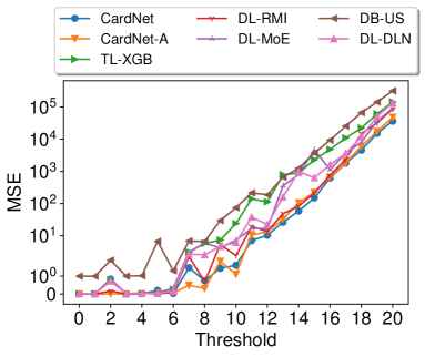
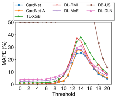
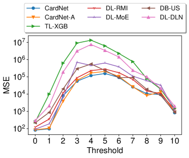
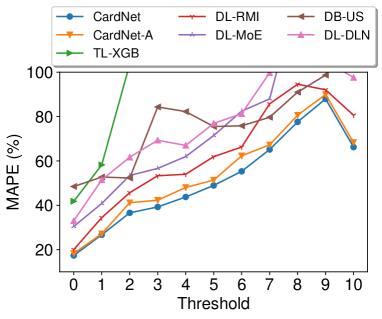
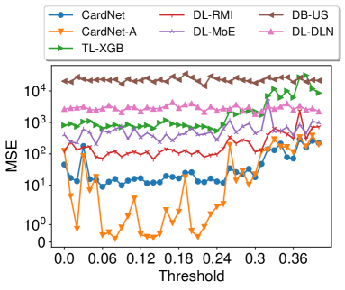
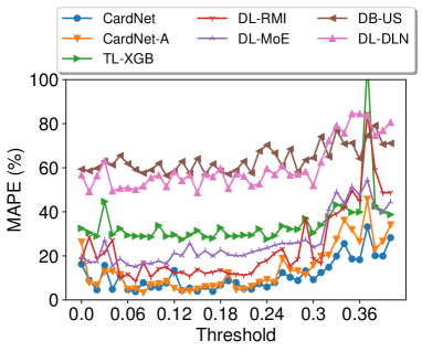
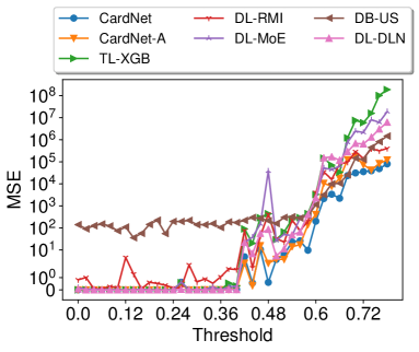
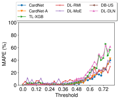
In Figure 5, we evaluate the accuracy with varying thresholds on the four default datasets. We compare with the following models: DB-US, TL-XGB, DL-DLN, DL-MoE, DL-RMI, the more accurate or monotonic models out of each category. The general trend is that the errors increase with the threshold, meaning that larger thresholds are harder. The exceptions are MAPE on Hamming distance and MSE on edit distance. The reason is that the cardinalities of some large thresholds tend to resemble for different queries, and regression models are more likely to predict well.

9.3. Estimation Efficiency

In Table 5, we show the average estimation time. We also report the time of running a state-of-the-art similarity selection algorithm (DBLP:journals/pvldb/QinX18, ; fastercovertree, ) to process queries to obtain the cardinality (referred to as SimSelect). The estimation time of CardNet is close to DL-RMI and faster than the database methods and TL-KDE. Thanks to the acceleration technique, CardNet-A becomes the runner-up, and its speed is close to the fastest model DL-DNN. CardNet-A is faster than running the similarity selection algorithms by at least 24 times.

9.4. Evaluation of Model Components

We evaluate the following components in our models: feature extraction, incremental prediction, variational auto-encoder (VAE), and dynamic training strategy. We use the following radio to measure the improvement by each component:

\displaystyle\gamma_{\xi}=\frac{\xi(\textsf{CardNet\{-A\}}_{\text{-C}})-\xi(\textsf{CardNet\{-A\}})}{\xi(\textsf{CardNet\{-A\}}_{\text{-C}})},

where $\xi\in\{\,\textsf{MAPE},\textsf{MSE}\,\text{mean q-error}\,\}$ , CardNet{-A} is our model CardNet or CardNet-A, and $\textsf{CardNet\{-A\}}_{\text{-C}}$ is CardNet{-A} with component C replaced by other options; e.g., $\textsf{CardNet\{-A\}}_{-\textsf{VAE}}$ is our model with VAE replaced. A positive $\gamma_{\xi}$ means the component has a positive effect in accuracy.

We consider the following replacement options: (1) For feature extraction, we adopt a character-level bidirectional LSTM to transfer a string to a dense representation for edit distance, a deep set model (zaheer2017deep, ) to transfer a set to its representation for Jaccard distance, and use the original record as input for Euclidean distance. Hamming distance is not repeatedly tested as we use original vectors as input. (2) For incremental prediction, we compare it with a deep neural network that takes as input the concatenation of $\mathbf{x^{\prime}}$ and the embedding of $\tau$ and outputs the cardinality. (3) For VAE, we compare it with an option that directly concatenates the binary representation and distance embeddings. (4) For dynamic training, we compare it with using only MSLE as loss, i.e., removing the second term on the right side of Equation 3. We report the $\gamma_{\xi}$ values on the four default datasets in Table 6. The effects of the four components in our models are all positive, ranging from 5% to 93% improvement of MSE , 5% to 60% improvement of MAPE, and 9% to 64% improvement of mean q-error. The most useful component is incremental prediction, with 38% to 93% performance improvement. This demonstrates that using incremental prediction on deep neural networks is significantly better than directly feeding neural networks with training data, in accord with what we have observed in Tables 3 and 4.

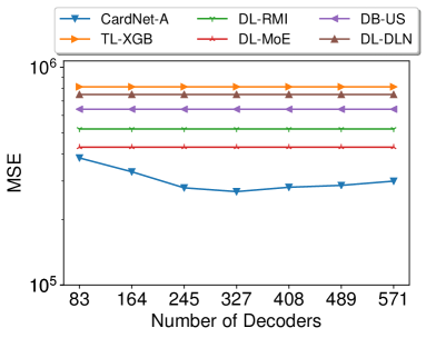
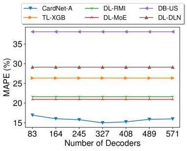
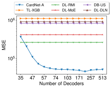
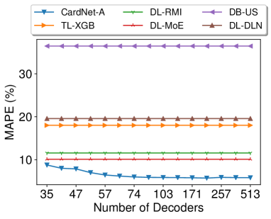
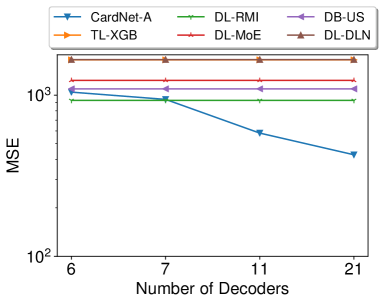
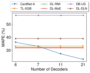
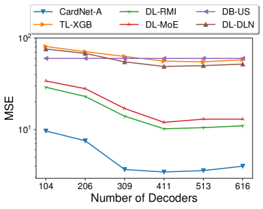
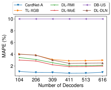
9.5. Number of Decoders

In Figure 6, we evaluate the accuracy by varying the number of decoders. In order to show the trend clearly, we use four datasets with large lengths or dimensionality, whose statistics is given in Table 7. As seen from the experimental results, we discover that using the largest $\tau_{\max}$ setting does not always lead to the best performance. E.g., on HM-Youtube, the best performance is achieved when $\tau_{max}=326$ (327 decoders). When there are too few decoders, the feature extraction becomes lossy and cannot successfully capture the semantic information of the original distance functions. As the number of decoders increases, the feature extraction becomes more effective to capture the semantics. On the other hand, the performance drops if we use an excessive number of decoders. This is because given a query, the cardinality only increases at a few thresholds (e.g., a threshold of 50 and 51 might produce the same cardinality). Using too many decoders will involve too many non-increasing points, posing difficulty in learning the regression model.

Table 7. Statistics of datasets with high dimensionality.

Dataset	Source	Process	Data Type	Attribute	# Record	$\ell_{max}$	$\ell_{avg}$	Distance	$\theta_{max}$
HM-Youtube	Youtube_Faces (URL:youtube-faces, )	normalize	real-valued vector	video	346,194	1770	1770	Euclidean	0.8
$\textsf{HM-GIST}_{2048}$	GIST (URL:gist, )	Spectral Hashing (weiss2009spectral, )	binary vector	image	982,677	2048	2048	Hamming	512
ED-DBLP	(URL:dblp, )	-	string	publication title	1,000,000	199	72.49	edit	20
JC-Wikipedia	Wikipedia (URL:wikipedia, )	3-gram	string	abstract	1,150,842	732	496.06	Jaccard	0.4

9.6. Model Size

Table 8 shows the storage sizes of the competitors on the four default datasets. DB-US does not need any storage and thus shows zero model size. TL-KDE has the smallest model size among the others, because it only stores the kernel instances for estimation. For deep learning models, DL-DNN has the smallest model size. Our model sizes range from 10 to 55 MB, smaller than the other deep models except DL-DNN.

9.7. Evaluation of Training

9.7.1. Training Time

Table 9 shows the training times of various models on the four default datasets. Traditional learning models are faster to train. Our models spend 2 – 4 hours, similar to other deep models. $\textsf{DL-DNNs}_{\tau}$ is the slowest since its has $(\tau_{max}+1)$ independently learned deep neural networks.

9.7.2. Varying the Size of Training Data

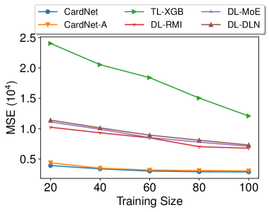
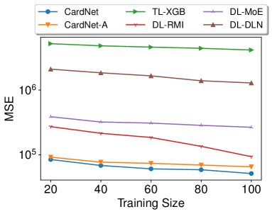
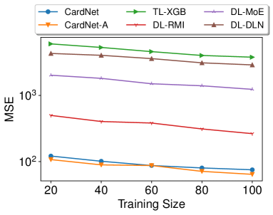
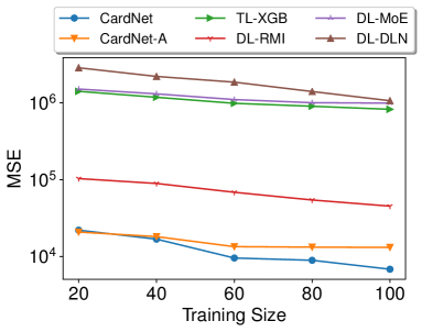
In Figure 7, we show the performance of different models by varying the scale of training examples from 20% to 100% of the original training data. We only plot MSE due to the page limitation. All the models have worse performance with fewer training data, but our models are more robust, showing moderate accuracy loss.

Table 8. Model size (MB).

Model	HM-ImageNet	ED-AMiner	JC-BMS	$\textsf{EU-Glove}_{300}$
DB-SE	10.4	31.2	39.4	86.2
DB-US	0.6	0.5	0.6	3.4
TL-XGB	36.4	36.4	48.8	63.2
TL-LGBM	32.6	32.8	45.4	60.4
TL-KDE	4.5	1.5	3.6	18.1
DL-DLN	28.4	75.4	28.6	64.4
DL-MoE	16.8	52.5	35.4	52.5
DL-RMI	57.7	84.8	54.6	66.1
DL-DNN	5.0	14.5	8.7	9.8
$\textsf{DL-DNNs}_{\tau}$	105.4	154.2	183.2	158.4
CardNet	9.6	40.2	16.4	23.8
CardNet-A	16.2	54.5	22.8	35.3

Table 9. Training time (hours).

Model	HM-ImageNet	ED-AMiner	JC-BMS	$\textsf{EU-Glove}_{300}$
TL-XGB	0.8	0.8	1.0	1.2
TL-LGBM	0.6	0.5	0.7	0.6
TL-KDE	0.3	0.3	0.5	0.6
DL-DLN	4.1	4.6	4.5	4.9
DL-MoE	2.7	3.5	3.8	3.8
DL-RMI	3.2	3.7	3.9	4.4
DL-DNN	1.2	1.5	1.7	1.8
$\textsf{DL-DNNs}_{\tau}$	15	12	12	20
CardNet	3.3	3.4	4.1	4.2
CardNet-A	1.7	2.2	2.4	2.6

9.8. Evaluation of Updates

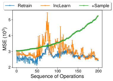
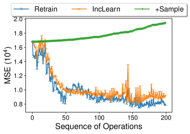
We generate a stream of 200 update operations, each with an insertion or deletion of 5 records. We compare three methods: IncLearn that utilizes incremental learning on CardNet-A, Retrain that retrains CardNet-A for each operation, and +Sample that performs sampling (DB-US) on the updated data and add the result to that of CardNet-A on the original data. Figure 8 plots the MSE on HM-ImageNet and $\textsf{EU-Glove}_{300}$ . We observe that in most cases, IncLearn has similar performance to Retrain and performs better than +Sample, especially when there are more updates. Compared to Retrain that spends several hours to retrain the model (Table 9), IncLearn only needs 1.2 – 1.5 minutes to perform incremental learning.

9.9. Evaluation of Long-tail Queries

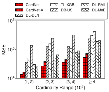
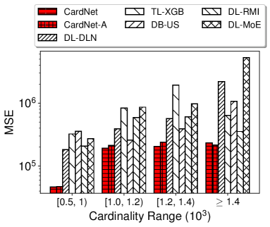
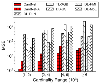
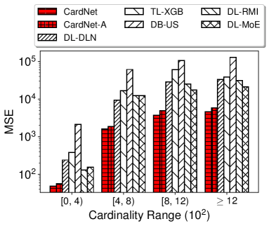
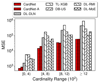
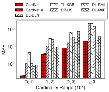
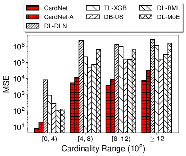
We compare the performance on long-tail queries, i.e., those having exceptionally large cardinalities ( $\geq$ 1000). They are outliers and a hard case of estimation. We divide queries into different cardinality groups by every thousand. Figure 9 shows the MSE on the four default datasets by varying cardinality groups. The MSE increases with cardinality for all the methods. This is expected since the larger the cardinality is, the more exceptional is the query (see Figure 1(b)). Our models outperform the others by 1 to 3 orders of magnitude. Moreover, the MSE growth rates of our models w.r.t. cardinality are smaller than the others, suggesting that our models are more robust against long-tail queries.

9.10. Generalizability

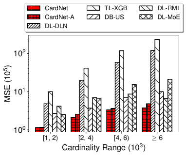
To show the generalizability of our models, we evaluate the performance on the queries that significantly differ from the records in the dataset and the training data. To prepare such queries, we first perform a $k$ -medoids clustering on the dataset, and then randomly generate 10,000 out-of-dataset queries and pick the top-2,000 ones having the largest sum of squared distance to the $k$ centroids. To prepare an out-of-dataset query, we generate a random query $q$ and accept it only if it is not in the dataset $\mathcal{D}$ . Specifically, (1) for binary vectors, $q[i]\sim\text{uniform}\{\,0,1\,\}$ ; (2) for strings, since AMiner and DBLP both contain author names, we take a random author name from the set $(\text{DBLP}\backslash\text{AMiner})$ ; (3) for sets, we generate a length $l\sim\text{uniform}[l_{\min},l_{\max}]$ , where $l_{\min}$ and $l_{\max}$ are the minimum and maximum set sizes in $\mathcal{D}$ , respectively, and then generate a random set of length $l$ sampled from the universe of all the elements in $\mathcal{D}$ ; (4) for real vectors, $q[i]\sim\text{uniform}[-1,1]$ . Figure 10 shows the MSE on the four default datasets by varying cardinality groups. The same trend is witnessed as we have seen for long-tail queries. Due to the use of VAE and dynamic training, our models always perform better than the other methods, especially for Jaccard distance. The results demonstrate that our models generalize well for out-of-dataset queries.

Table 10. Statistics of datasets for conjunctive query optimizer.

Dataset	Source	Attributes	# Records	$\theta_{\min}$	$\theta_{\max}$
AMiner-Publication	(URL:aminer, )	title, authors, affiliations, venue, abstract	2,092,356	0.2	0.5
AMiner-Author	(URL:aminer, )	name, affiliations, research interests	1,712,433	0.2	0.5
IMDB-Movie	(URL:imdb, )	title type, primary title, original title, genres	6,250,486	0.2	0.5
IMDB-Actor	(URL:imdb, )	primary name, primary profession	9,822,710	0.2	0.5

9.11. Performance in a Query Optimizer

9.11.1. Conjunctive Euclidean Distance Query

We consider a case study of conjunctive queries. Four textual datasets with multiple attributes are used (statistics shown in Table 10). Given a dataset, we convert each attribute to a word embedding (768 dimensions) by Sentence-BERT (DBLP:conf/emnlp/ReimersG19, ). A query is a conjunction of Euclidean distance predicates (a.k.a. high-dimensional range predicates (DBLP:journals/vldb/LinJF94, )) on normalized word embeddings, with thresholds uniformly sampled from $[0.2,0.5]$ ; e.g., “ $\textsf{EU}(\text{name})\leq 0.25$ AND $\textsf{EU}(\text{affiliations})\leq 0.4$ AND $\textsf{EU}(\text{research interests})\leq 0.45$ ”, where $\textsf{EU}()$ measures the Euclidean distance between the embeddings of a query and a database record. Such queries can be used for entity matching as blocking rules (DBLP:conf/sigmod/GokhaleDDNRSZ14, ; DBLP:conf/sigmod/DasCDNKDARP17, ).

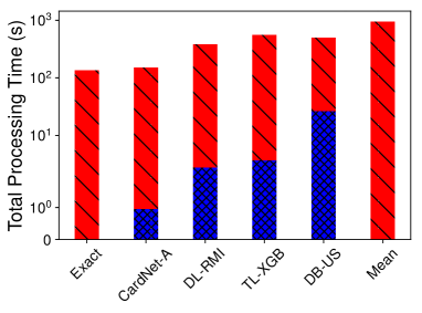
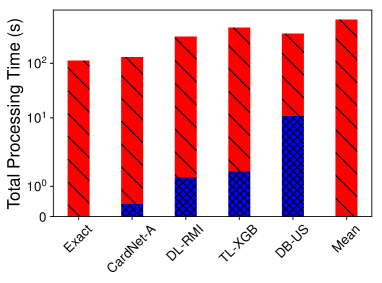
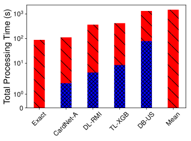
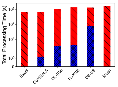
To process a query, we first find the records that satisfy one predicate by index lookup (by a cover tree (fastercovertree, )), and then check other predicates on the fly. We estimate for each predicate and pick the one with the smallest cardinality for index lookup. We compare CardNet-A with: (1) DB-US, sampling ratio tuned for fastest query processing speed; (2) TL-XGB; (3) DL-RMI; (4) Mean, which returns the same cardinality for a given threshold; each threshold is quantized to an integer in $[0,255]$ using the threshold transformation in Section 4.4, and then we offline generate 10,000 random queries for each integer in $[0,255]$ and take the mean; and (5) Exact, an oracle that instantly returns the exact cardinality.

Figure 11 reports the processing time of 1,000 queries. The time is broken down to cardinality estimation (in blue) and postprocessing (in red, including index lookup and on-the-fly check). We observe: (1) more accurate cardinality estimation (as we have seen in Section 9.2) contributes to faster query processing speed; (2) cardinality estimation spends much less time than postprocessing; (3) uniform estimation (Mean) has the slowest overall speed; (4) deep learning performs better than database and traditional learning methods in both estimation and overall speeds; (5) except Exact, CardNet-A is the fastest and most accurate in estimation, and its overall speed is also the fastest (by 1.7 to 3.3 times faster than the runner-up DL-RMI) and even close to Exact.

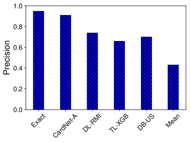
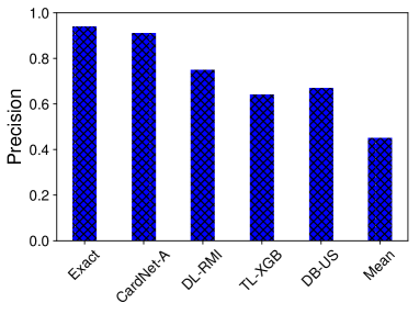
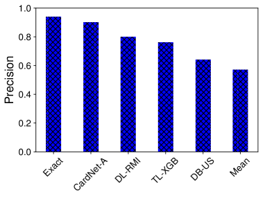
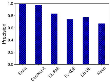
In Figure 12, we show the precision of query planning, i.e., the percentage of queries on which a method picks the fastest (excluding estimation time) plan. The result is in accord with what we have observed in Figure 11. The precision of CardNet-A ranges from 90% to 96%, second only to Exact. The gap between CardNet-A and DL-RMI is within 20%, but results in the speedup of 1.7 to 3.3 times, showcasing the effect of correct query planning. We also observe that Exact is not 100% precise, though very close, indicating that smallest cardinality does not always yield the best query plan. Future work on cost estimation may further improve query processing.

Table 11. Statistics of datasets for Hamming distance query optimizer.

Dataset	Source	Process	Domain	# Records	$\ell$	$\theta_{max}$
HM-PubChem	(URL:pubchem, )	-	biological sequence	1,000,000	881	32
HM-UQVideo	(DBLP:journals/tmm/SongYHSL13, )	multiple feature hashing (DBLP:journals/tmm/SongYHSL13, )	video embedding	1,000,000	128	12
HM-fastText	(URL:fasttext, )	spectral hashing (weiss2009spectral, )	word embedding	999,999	256	24
HM-EMNIST	(DBLP:conf/ijcnn/CohenATS17, )	image binarization	image pixel	814,255	784	32

9.11.2. Hamming Distance Query

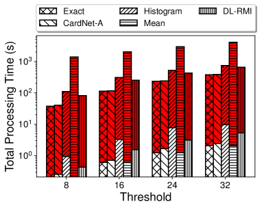
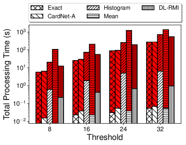
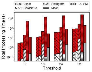
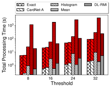
We also consider a case study of the GPH algorithm (qin2018gph, ), which processes Hamming distance queries over high dimensional vectors through a query optimizer. To cope with the high dimensionality, the algorithm answers a query $q$ by dividing it into $m$ non-overlapping parts and allocating a threshold (with dynamic programming) to each part using the pigeonhole principle. Each part itself is a Hamming distance selection query that can be answered by bit enumeration and index lookup. The union of the answers of the $m$ parts are the candidates of $q$ . To allocate thresholds and hence to achieve small query processing cost, a query optimizer is used to minimize the sum of estimated cardinalities of the $m$ parts. We compare CardNet-A with the following options: (1) Histogram, the histogram estimator in (qin2018gph, ); (2) DL-RMI; (3) Mean, an naive estimator that returns the same cardinality for a given threshold (for each threshold, we offline generate 10,000 random queries and take the mean); and (4) Exact, an oracle that instantly returns the exact cardinality. We use four datasets. The statistics is given in Table 11, where $\ell$ denotes the dimensionality. The records are converted to binary vectors as per the process in the table. We set each part to 32 bits (the last part is smaller if not divisible).

Figure 13 reports the processing time of 1,000 queries by varying thresholds from 8 to 32 on the four datasets. The time is broken down to threshold allocation time (in white, which contains cardinality estimation) and postprocessing time (in red). The performance of CardNet-A is very close to Exact and faster than Histogram by 1.6 to 4.9 times speedup. DL-RMI is slightly faster than Histogram. Mean is much slower (typically one order of magnitude) than other methods, suggesting that cardinality estimation is important for this application. The threshold allocation (including cardinality estimation) spends less time than the subsequent query processing. CardNet-A also performs better than Histogram in threshold allocation. This is because (1) CardNet-Aitself is faster in estimation, and (2) the more accuracy makes the dynamic programming-based allocation terminate earlier.

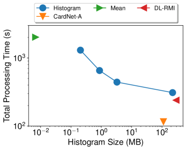
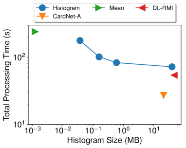
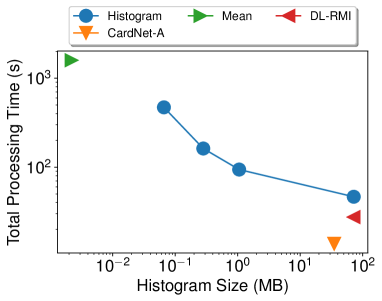
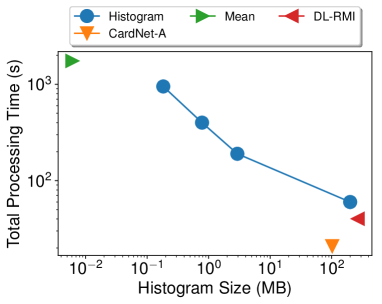
Next we fix the threshold at 50% of the maximum threshold in Figure 13 and vary the size of the histogram. Figure 14 reports the average query processing time. The positions of other methods (except Exact) are also marked in the figure. As expected, the query processing time reduces when using larger histograms. However, the speed is still 1.6 to 2.6 times slower than CardNet-A even if the size of the histogram exceeds the model size of CardNet-A (see the rightmost point of Histogram). This result showcases the superiority of our model compared to the traditional database method in an application of cardinality estimation of similarity selection.

10. Conclusion

We investigated utilizing deep learning for cardinality estimation of similarity selection. Observing the challenges of this problem and the advantages of using deep learning, we designed a method composed of two components. The feature extraction component transforms original data and threshold to Hamming space, hence to support any data types and distance functions. The regression component estimates the cardinality in the Hamming space based on a deep learning model. We exploited the incremental property of cardinality to output monotonic results and devised a set of encoder and decoders that estimates the cardinality for each distance value. We developed a training strategy tailored to our model and proposed optimization techniques to speed up estimation. We discussed incremental learning for updates. The experimental results demonstrated the accuracy, efficiency, and generalizability of the proposed method as well as the effectiveness of integrating our method to a query optimizer.

Acknowledgments

This work was supported by JSPS 16H01722, 17H06099, 18H04093, and 19K11979, NSFC 61702409, CCF DBIR2019001A, NKRDP of China 2018YFB1003201, ARC DE190100663, DP170103710, and DP180103411, and D2D CRC DC25002 and DC25003. The Titan V was donated by Nvidia. We thank Rui Zhang (the University of Melbourne) for his precious comments.

References

[1] http://www.image-net.org/.
[2] https://pubchem.ncbi.nlm.nih.gov/.
[3] https://aminer.org/.
[4] https://dblp2.uni-trier.de/.
[5] https://www.kdd.org/kdd-cup/view/kdd-cup-2000.
[6] https://nlp.stanford.edu/projects/glove/.
[7] http://www.cs.tau.ac.il/~wolf/ytfaces/index.html.
[8] http://horatio.cs.nyu.edu/mit/tiny/data/index.html.
[9] https://wiki.dbpedia.org/services-resources/documentation/datasets.
[10] https://www.imdb.com/interfaces/.
[11] https://fasttext.cc/docs/en/english-vectors.html.
[12] C. Anagnostopoulos and P. Triantafillou. Query-driven learning for predictive analytics of data subspace cardinality. ACM Transactions on Knowledge Discovery from Data, 11(4):47, 2017.
[13] Y. Bengio, A. C. Courville, and P. Vincent. Representation learning: A review and new perspectives. IEEE Transactions on Pattern Analysis and Machine Intelligence, 35(8):1798–1828, 2013.
[14] W. Cai, M. Balazinska, and D. Suciu. Pessimistic cardinality estimation: Tighter upper bounds for intermediate join cardinalities. In SIGMOD, pages 18–35, 2019.
[15] Z. Cao, M. Long, J. Wang, and S. Y. Philip. Hashnet: Deep learning to hash by continuation. In ICCV, pages 5609–5618, 2017.
[16] T. Chen and C. Guestrin. Xgboost: A scalable tree boosting system. In KDD, pages 785–794, 2016.
[17] J. P. Chiu and E. Nichols. Named entity recognition with bidirectional lstm-cnns. Transactions of the Association for Computational Linguistics, 4:357–370, 2016.
[18] G. Cohen, S. Afshar, J. Tapson, and A. van Schaik. EMNIST: extending MNIST to handwritten letters. In IJCNN, pages 2921–2926, 2017.
[19] H. Daniels and M. Velikova. Monotone and partially monotone neural networks. IEEE Transactions on Neural Networks, 21(6):906–917, 2010.
[20] S. Das, P. S. G. C., A. Doan, J. F. Naughton, G. Krishnan, R. Deep, E. Arcaute, V. Raghavendra, and Y. Park. Falcon: Scaling up hands-off crowdsourced entity matching to build cloud services. In SIGMOD, pages 1431–1446, 2017.
[21] A. Dasgupta, X. Jin, B. Jewell, N. Zhang, and G. Das. Unbiased estimation of size and other aggregates over hidden web databases. In SIGMOD, pages 855–866, 2010.
[22] M. Datar, N. Immorlica, P. Indyk, and V. S. Mirrokni. Locality-sensitive hashing scheme based on p-stable distributions. In SOCG, pages 253–262, 2004.
[23] B. Ding, S. Das, R. Marcus, W. Wu, S. Chaudhuri, and V. R. Narasayya. AI meets AI: leveraging query executions to improve index recommendations. In SIGMOD, pages 1241–1258, 2019.
[24] A. Dutt, C. Wang, A. Nazi, S. Kandula, V. R. Narasayya, and S. Chaudhuri. Selectivity estimation for range predicates using lightweight models. PVLDB, 12(9):1044–1057, 2019.
[25] M. M. Fard, K. Canini, A. Cotter, J. Pfeifer, and M. Gupta. Fast and flexible monotonic functions with ensembles of lattices. In NIPS, pages 2919–2927, 2016.
[26] E. Garcia and M. Gupta. Lattice regression. In NIPS, pages 594–602, 2009.
[27] A. Gionis, P. Indyk, and R. Motwani. Similarity search in high dimensions via hashing. In VLDB, pages 518–529, 1999.
[28] C. Gokhale, S. Das, A. Doan, J. F. Naughton, N. Rampalli, J. W. Shavlik, and X. Zhu. Corleone: hands-off crowdsourcing for entity matching. In SIGMOD, pages 601–612, 2014.
[29] M. Gupta, A. Cotter, J. Pfeifer, K. Voevodski, K. Canini, A. Mangylov, W. Moczydlowski, and A. Van Esbroeck. Monotonic calibrated interpolated look-up tables. The Journal of Machine Learning Research, 17(1):3790–3836, 2016.
[30] P. J. Haas and A. N. Swami. Sequential Sampling Procedures for Query Size Estimation, volume 21. ACM, 1992.
[31] S. Hasan, S. Thirumuruganathan, J. Augustine, N. Koudas, and G. Das. Multi-attribute selectivity estimation using deep learning. CoRR, abs/1903.09999, 2019.
[32] M. Heimel, M. Kiefer, and V. Markl. Self-tuning, GPU-accelerated kernel density models for multidimensional selectivity estimation. In SIGMOD, pages 1477–1492, 2015.
[33] O. Ivanov and S. Bartunov. Adaptive cardinality estimation. arXiv preprint arXiv:1711.08330, 2017.
[34] M. Izbicki and C. R. Shelton. Faster cover trees. In ICML, pages 1162–1170, 2015.
[35] H. Jiang. Uniform convergence rates for kernel density estimation. In ICML, pages 1694–1703, 2017.
[36] L. Jin, C. Li, and R. Vernica. SEPIA: estimating selectivities of approximate string predicates in large databases. The VLDB Journal, 17(5):1213–1229, 2008.
[37] M. Johnson, M. Schuster, Q. V. Le, M. Krikun, Y. Wu, Z. Chen, N. Thorat, F. B. Viégas, M. Wattenberg, G. Corrado, M. Hughes, and J. Dean. Google’s multilingual neural machine translation system: Enabling zero-shot translation. Transactions of the Association for Computational Linguistics, 5:339–351, 2017.
[38] G. Ke, Q. Meng, T. Finley, T. Wang, W. Chen, W. Ma, Q. Ye, and T. Liu. Lightgbm: A highly efficient gradient boosting decision tree. In NIPS, pages 3149–3157, 2017.
[39] R. Kemker, M. McClure, A. Abitino, T. L. Hayes, and C. Kanan. Measuring catastrophic forgetting in neural networks. In AAAI, pages 3390–3398, 2018.
[40] D. P. Kingma and M. Welling. Auto-encoding variational bayes. arXiv preprint arXiv:1312.6114, 2013.
[41] A. Kipf, T. Kipf, B. Radke, V. Leis, P. A. Boncz, and A. Kemper. Learned cardinalities: Estimating correlated joins with deep learning. In CIDR, 2019.
[42] T. Kraska, M. Alizadeh, A. Beutel, E. H. Chi, A. Kristo, G. Leclerc, S. Madden, H. Mao, and V. Nathan. Sagedb: A learned database system. In CIDR, 2019.
[43] T. Kraska, A. Beutel, E. H. Chi, J. Dean, and N. Polyzotis. The case for learned index structures. In SIGMOD, pages 489–504, 2018.
[44] S. Krishnan, Z. Yang, K. Goldberg, J. Hellerstein, and I. Stoica. Learning to optimize join queries with deep reinforcement learning. arXiv preprint arXiv:1808.03196, 2018.
[45] H. Lee, R. T. Ng, and K. Shim. Extending q-grams to estimate selectivity of string matching with low edit distance. In VLDB, pages 195–206, 2007.
[46] H. Lee, R. T. Ng, and K. Shim. Power-law based estimation of set similarity join size. PVLDB, 2(1):658–669, 2009.
[47] H. Lee, R. T. Ng, and K. Shim. Similarity join size estimation using locality sensitive hashing. PVLDB, 4(6):338–349, 2011.
[48] V. Leis, B. Radke, A. Gubichev, A. Kemper, and T. Neumann. Cardinality estimation done right: Index-based join sampling. In CIDR, 2017.
[49] G. Li, J. He, D. Deng, and J. Li. Efficient similarity join and search on multi-attribute data. In SIGMOD, pages 1137–1151, 2015.
[50] P. Li and C. König. b-bit minwise hashing. In WWW, pages 671–680, 2010.
[51] K. Lin, H. V. Jagadish, and C. Faloutsos. The tv-tree: An index structure for high-dimensional data. The VLDB Journal, 3(4):517–542, 1994.
[52] R. J. Lipton and J. F. Naughton. Query size estimation by adaptive sampling. In PODS, pages 40–46, 1990.
[53] H. Liu, M. Xu, Z. Yu, V. Corvinelli, and C. Zuzarte. Cardinality estimation using neural networks. In CSSE, pages 53–59, 2015.
[54] R. Marcus and O. Papaemmanouil. Deep reinforcement learning for join order enumeration. In aiDM@SIGMOD, pages 3:1–3:4, 2018.
[55] R. C. Marcus, P. Negi, H. Mao, C. Zhang, M. Alizadeh, T. Kraska, O. Papaemmanouil, and N. Tatbul. Neo: A learned query optimizer. PVLDB, 12(11):1705–1718, 2019.
[56] R. C. Marcus and O. Papaemmanouil. Plan-structured deep neural network models for query performance prediction. PVLDB, 12(11):1733–1746, 2019.
[57] M. Mattig, T. Fober, C. Beilschmidt, and B. Seeger. Kernel-based cardinality estimation on metric data. In EDBT, pages 349–360, 2018.
[58] A. Mazeika, M. H. Böhlen, N. Koudas, and D. Srivastava. Estimating the selectivity of approximate string queries. ACM Transactions on Database Systems, 32(2):12, 2007.
[59] M. McCloskey and N. J. Cohen. Catastrophic interference in connectionist networks: The sequential learning problem. In Psychology of learning and motivation, volume 24, pages 109–165. Elsevier, 1989.
[60] J. Ortiz, M. Balazinska, J. Gehrke, and S. S. Keerthi. Learning state representations for query optimization with deep reinforcement learning. In DEEM@SIGMOD, pages 4:1–4:4, 2018.
[61] J. Ortiz, M. Balazinska, J. Gehrke, and S. S. Keerthi. An empirical analysis of deep learning for cardinality estimation. CoRR, abs/1905.06425, 2019.
[62] H. Park and L. Stefanski. Relative-error prediction. Statistics & Probability Letters, 40(3):227–236, 1998.
[63] J. Qin, Y. Wang, C. Xiao, W. Wang, X. Lin, and Y. Ishikawa. GPH: Similarity search in hamming space. In ICDE, pages 29–40, 2018.
[64] J. Qin and C. Xiao. Pigeonring: A principle for faster thresholded similarity search. PVLDB, 12(1):28–42, 2018.
[65] N. Reimers and I. Gurevych. Sentence-bert: Sentence embeddings using siamese bert-networks. In EMNLP-IJCNLP, pages 3980–3990, 2019.
[66] O. Russakovsky, J. Deng, H. Su, J. Krause, S. Satheesh, S. Ma, Z. Huang, A. Karpathy, A. Khosla, M. Bernstein, A. C. Berg, and L. Fei-Fei. ImageNet Large Scale Visual Recognition Challenge. International Journal of Computer Vision, 115(3):211–252, 2015.
[67] N. Shazeer, A. Mirhoseini, K. Maziarz, A. Davis, Q. Le, G. Hinton, and J. Dean. Outrageously large neural networks: The sparsely-gated mixture-of-experts layer. arXiv preprint arXiv:1701.06538, 2017.
[68] K. Sohn, H. Lee, and X. Yan. Learning structured output representation using deep conditional generative models. In NIPS, pages 3483–3491, 2015.
[69] J. Song, Y. Yang, Z. Huang, H. T. Shen, and J. Luo. Effective multiple feature hashing for large-scale near-duplicate video retrieval. IEEE Transactions on Multimedia, 15(8):1997–2008, 2013.
[70] J. Sun and G. Li. An end-to-end learning-based cost estimator. PVLDB, 13(3):307–319, 2019.
[71] I. Trummer. Exact cardinality query optimization with bounded execution cost. In SIGMOD, pages 2–17, 2019.
[72] M. Tschannen, O. Bachem, and M. Lucic. Recent advances in autoencoder-based representation learning. CoRR, abs/1812.05069, 2018.
[73] Y. Weiss, A. Torralba, and R. Fergus. Spectral hashing. In NIPS, pages 1753–1760, 2009.
[74] L. Woltmann, C. Hartmann, M. Thiele, D. Habich, and W. Lehner. Cardinality estimation with local deep learning models. In aiDM@SIGMOD, pages 5:1–5:8, 2019.
[75] W. Wu, J. F. Naughton, and H. Singh. Sampling-based query re-optimization. In SIGMOD, pages 1721–1736, 2016.
[76] X. Wu, M. Charikar, and V. Natchu. Local density estimation in high dimensions. In ICML, pages 5293–5301, 2018.
[77] Z. Yang, E. Liang, A. Kamsetty, C. Wu, Y. Duan, X. Chen, P. Abbeel, J. M. Hellerstein, S. Krishnan, and I. Stoica. Selectivity estimation with deep likelihood models. CoRR, abs/1905.04278, 2019.
[78] S. You, D. Ding, K. Canini, J. Pfeifer, and M. Gupta. Deep lattice networks and partial monotonic functions. In NIPS, pages 2981–2989, 2017.
[79] M. Zaheer, S. Kottur, S. Ravanbakhsh, B. Poczos, R. R. Salakhutdinov, and A. J. Smola. Deep sets. In NIPS, pages 3391–3401, 2017.
[80] H. Zhang and Q. Zhang. Embedjoin: Efficient edit similarity joins via embeddings. In KDD, pages 585–594, 2017.
[81] J. Zhang, Y. Liu, K. Zhou, G. Li, Z. Xiao, B. Cheng, J. Xing, Y. Wang, T. Cheng, L. Liu, M. Ran, and Z. Li. An end-to-end automatic cloud database tuning system using deep reinforcement learning. In SIGMOD, pages 415–432, 2019.
[82] W. Zhang, K. Gao, Y. Zhang, and J. Li. Efficient approximate nearest neighbor search with integrated binary codes. In ACM Multimedia, pages 1189–1192, 2011.
[83] Z. Zhao, R. Christensen, F. Li, X. Hu, and K. Yi. Random sampling over joins revisited. In SIGMOD, pages 1525–1539, 2018.