Fast Fair Regression via Efficient Approximations of Mutual Information

Abstract

Most work in algorithmic fairness to date has focused on discrete outcomes, such as deciding whether to grant someone a loan or not. In these classification settings, group fairness criteria such as independence, separation and sufficiency can be measured directly by comparing rates of outcomes between subpopulations. Many important problems however require the prediction of a real-valued outcome, such as a risk score or insurance premium. In such regression settings, measuring group fairness criteria is computationally challenging, as it requires estimating information-theoretic divergences between conditional probability density functions. This paper introduces fast approximations of the independence, separation and sufficiency group fairness criteria for regression models from their (conditional) mutual information definitions, and uses such approximations as regularisers to enforce fairness within a regularised risk minimisation framework. Experiments in real-world datasets indicate that in spite of its superior computational efficiency our algorithm still displays state-of-the-art accuracy$/$fairness tradeoffs.

1 Introduction

A machine learning algorithm trained with a standard objective such as maximum accuracy can produce behaviours that people, including those affected by its decisions, consider unfair. Algorithmic group fairness seeks to address this problem by defining protected attributes such as age, race or gender, and introducing mathematical fairness measures to enable assessment and potential amelioration of unfair treatment or outcomes. Many fairness measures have been proposed in the literature, but most can be posed as specialisations of three general criteria, independence, separation and sufficiency, that can be cleanly and intuitively defined in terms of statistical independence (Barocas et al., 2019).

To date, the algorithmic fairness literature has mainly focused on classification problems, where the decisions of a system are binary or categorical, such as predicting who should be released on bail (Angwin et al., 2016), or who should be audited for a potentially fraudulent tax return. In this setting, fairness measures are straightforward to compute based on the fraction of each group that were correctly or incorrectly selected or omitted.

However, there are many important problems which involve a real-valued prediction, such as how much to lend someone on a credit card or home loan, or how much to charge for an insurance premium. In such continuous settings the aforementioned fairness criteria are generally intractable to evaluate, and few attempts have been made in this direction (Agarwal et al., 2019; Berk et al., 2017; Fitzsimons et al., 2019).

In this paper, we

• introduce a technique that produces fast approximations of independence, separation and sufficiency group fairness criteria in a regression setting based on (conditional) mutual information. This technique is agnostic to the regression algorithms used.

• incorporate the resulting approximations as fairness regularisers in a regression setting, thus enabling us to trade-off accuracy and fairness within a regularised risk minimisation framework.

• empirically compare our method with a state-of-the-art approach using real data and benchmarking directly against these three fairness criteria. To the best of our knowledge we offer the first investigation of the trade-offs between accuracy and satisfaction of all of these fairness criteria in a regression setting.

1.1 Related Work

Predictive fairness measures date back more than fifty years in the context of testing and hiring, as summarised by Hutchinson & Mitchell (2019). Of particular relevance to our work are the measures of regression fairness based on (partial) correlations between the predicted score, the target variable and the demographic group of applicants, as derived in (Cleary, 1968; Darlington, 1971). These measures can be interpreted as relaxations of the independence, separation and sufficiency criteria under the assumption that the outcome, prediction and group are jointly Gaussian distributed. Propensity score stratification techniques have also been used to decrease the separation of the protected class for linear regressors in (Calders et al., 2013). Berk et al. (2017) propose fairness objectives that address separation using convex regularisers. One of these regularisers (‘group’) permits cancelling of model errors within a group, addressing an imbalance in expectation, while the other (‘individual’) does not. Fitzsimons et al. (2019) have developed an inprocessing technique for kernel machines and decision tree regressors with a focus on satisfying (a relaxation of) the independence criterion. Agarwal et al. (2019) propose methods for fair regression of real-valued outputs for both the independence criterion and a bounded group loss criterion. For bounded group loss the approach is based on weighted loss minimisation, whereas for the independence criterion the algorithm proposed involves a reduction to classification based on a suitable discretisation of the real-valued output space. Williamson & Menon (2019) proposed that risk measures from mathematical finance generalise to fairness measures by imposing that the distribution of losses across subgroups are commensurate. Of particular interest, the conditional value at risk measure leads to a convex inprocessing technique for both regression and classification problems.

Mutual information (MI) has also previously been considered in the context of fair supervised learning. Kamishima et al. (2012) use normalised MI to asses fairness in their normalised prejudice index (NPI). Their focus is on binary classification with binary sensitive attributes, and the NPI is based on the independence fairness criterion. In such a setting mutual information is readily computable empirically from confusion matrices. This work is generalised in (Fukuchi et al., 2015) for use in regression models by using a neutrality measure, which the authors show is equivalent to the independence criterion. They then use this neutrality measure to create inprocessing techniques for linear and logistic regression algorithms. Similarly, Ghassami et al. (2018) take an information theoretic approach to creating an optimisation algorithm that returns a predictor score that is fair (up to some $\epsilon$) with respect to the separation criterion. Though they have left as future work to test an implementation of this algorithm on real data. In constrast, the focus in our paper is to present fast and scalable methods of approximating conditional mutual information specifically tailored to encoding the independence, separation and sufficiency criteria within a learning algorithm.

2 Problem Formulation

We consider a predictor with target set, $\mathcal{Y}$, feature set, $\mathcal{X}$, and a sensitive attribute set, $\mathcal{A}$ and corresponding random variables $Y$, $A$ and $X$. Our data is assumed drawn from some distribution over $\mathcal{Y}\times\mathcal{X}$ ($\mathcal{A}$ is a subset of $\mathcal{X}$). Here $f$ is a prediction function $f:\mathcal{X}\to\mathcal{S}$ that produces scores $S=f\!\left({X,\boldsymbol{\theta}}\right)$, with parameters $\boldsymbol{\theta}\in\Theta$. For the purposes of this paper we will treat $S$ as a random variable drawn from a distribution over $\mathcal{S}$, and also that $\mathcal{S}=\mathcal{Y}$.

We are specifically interested in approximating independence, separation and sufficiency, a selection that subsumes many other measures as relaxations or special cases (Barocas et al., 2019). These can be defined in terms of independence or conditional independence statements,

Independence:

$$\qquad S\bot A\Leftrightarrow\mathrm{P}\!\left({S,A}\right)=\mathrm{P}\!\left({S}\right)\mathrm{P}\!\left({A}\right),$$ (1)

Separation:

$$\qquad S\bot A~{}|~{}Y\Leftrightarrow\mathrm{P}\!\left({S,A}|{Y}\right)=\mathrm{P}\!\left({S}|{Y}\right)\mathrm{P}\!\left({A}|{Y}\right),$$ (2)

Sufficiency:

$$\qquad Y\bot A~{}|~{}S\Leftrightarrow\mathrm{P}\!\left({Y,A}|{S}\right)=\mathrm{P}\!\left({Y}|{S}\right)\mathrm{P}\!\left({A}|{S}\right).$$ (3)

Strictly speaking, all of these distributions are different functions that take instances of random variables as input, e.g. $\mathrm{P}_{A|S}(A=a|S=s)$. In the interest of being concise, we will assume the reader can infer the specific probability distribution given either random variable inputs in the generic case, $\mathrm{P}\!\left({A}|{S}\right)$, or specific instances of them, $\mathrm{P}\!\left({a}|{s}\right)$, where appropriate.

Rather than constraining the predictor such that these conditions be exactly satisfied, we would usually define a continuous measure of the degree to which they are satisfied. This admits a balancing of priorities between these and other measures such as accuracy.

In the classification setting where $Y$, $S$ and $A$ are all categorical, these conditional probabilities can be empirically estimated from confusion matrices between $Y$ and $S$ for each protected subgroup  (Barocas et al., 2019). In a regression setting, however, they become continuous density functions, and we are required to either assume a parametric form for them, or numerically estimate the densities using methods such as kernel density estimation (Hastie et al., 2001). Others have simplified these criteria using conditional expectation instead of conditional probability (Calders et al., 2013; Zafar et al., 2015; Fitzsimons et al., 2019). This approach however can fail to capture important effects that can still lead to harm, such as groups with different score variances.

Our primary aim in this paper is to create techniques that tractably approximate the three above criteria of group fairness in a way that is agnostic to the predictor used to generate the score, $S$, and that can be incorporated into a regression learning objective. More formally,

Problem Statement.

Derive methods that can approximate the fairness criteria independence, separation and sufficiency, for $\mathcal{Y}\subseteq\real$ and $\mathcal{S}\subseteq\real$, in the case of binary or categorical sensitive attributes, $\mathcal{A}=\{0,\ldots,K\}$, $K\geq 1$, and incorporate the resulting approximations as regularisers into a regression learning objective.

3 Measuring Group Fairness

A natural approach to measuring the fairness criteria in (1)-(3) is to calculate the (conditional) mutual information (MI) (Gel’fand & Yaglom, 1957; Cover & Thomas, 2006) between the relevant variables. For instance, to asses the independence criterion from (1), we can calculate the MI between $S$ and $A$ (Fukuchi et al., 2015),

$$\mathrm{I}\!\left[{S};{A}\right]=\int_{\mathcal{S}}\sum_{a\in\mathcal{A}}\mathrm{P}\!\left({s,a}\right)\log\frac{\mathrm{P}\!\left({s,a}\right)}{\mathrm{P}\!\left({s}\right)\mathrm{P}\!\left({a}\right)}\mathrm{d}{s}.$$ (4)

Here we can see that if we achieve perfect fairness as defined by independence, we have $\mathrm{P}\!\left({S,A}\right)=\mathrm{P}\!\left({S}\right)\mathrm{P}\!\left({A}\right)$, which implies $\mathrm{I}\!\left[{S};{A}\right]=0$; otherwise MI will be positive. We can also normalise MI by one of its many known upper bounds so that it takes values in $[0,1]$. One useful upper bound in this context is the entropy of the sensitive attribute, $\mathrm{H}\!\left[{A}\right]$, that gives the normalised measure,

$$\tilde{\mathrm{I}}\!\left[{S};{A}\right]=\frac{\mathrm{I}\!\left[{S};{A}\right]}{\mathrm{H}\!\left[{A}\right]},~{}~{}\text{where}~{}\mathrm{H}\!\left[{A}\right]=-\sum_{a\in\mathcal{A}}\mathrm{P}\!\left({a}\right)\log\mathrm{P}\!\left({a}\right).$$ (5)

The reason for using $\mathrm{H}\!\left[{A}\right]$ as a normaliser is because MI and entropy are related through $\mathrm{I}\!\left[{S};{A}\right]=\mathrm{H}\!\left[{A}\right]-\mathrm{H}\!\left[{A}|{S}\right]$, where $\mathrm{H}\!\left[{A}|{S}\right]$ is conditional entropy, and is a measure of how much of the information of $P(A)$ is encoded by $P(S)$. When $\tilde{\mathrm{I}}\!\left[{S};{A}\right]=1$ we have that $\mathrm{H}\!\left[{A}|{S}\right]=0$, so the distribution of $S$ completely encodes all information about $A$. This would be maximally unfair according to the independence criterion of fairness, since we can completely recover all information about the sensitive attribute from the model’s predictions.

Since we do not have access to these probability densities we have to resort to approximating $\tilde{\mathrm{I}}\!\left[{S};{A}\right]$ from samples. Many general approximation methods for mutual information exist in the literature, for example the popular “KSG” method (Kraskov et al., 2004) and improvements (Gao et al., 2018), and recent work including (Belghazi et al., 2018). When considering categorical protected attributes in a regression context, methods that can handle mixed categorical/continuous distributions are necessary, for example (Gao et al., 2017), which we do compare against. However, these methods have runtime performance and computational complexity that makes them unsuitable for use in a regularisation term during training. This motivates our proposal of a fast approximation method that handles the mixed categorical/continuous case resulting from a discrete protected attribute and a continuous, real-valued outcome variable.

We start by noting that $\mathrm{H}\!\left[{A}\right]$ is easy to approximate empirically,

$$\mathrm{H}\!\left[{A}\right]\approx-\sum_{a\in\mathcal{A}}\frac{n_{a}}{n}\log\frac{n_{a}}{n},$$ (6)

where $n_{a}$ is the number of instances that have sensitive attribute $A=a$, and $n$ is the total number of instances in the dataset.

In order to approximate $\mathrm{I}\!\left[{S};{A}\right]$, note it can be rewritten as

$$\mathrm{I}\!\left[{S};{A}\right]=\int_{\mathcal{S}}\sum_{a\in\mathcal{A}}\mathrm{P}\!\left({s,a}\right)\log\frac{\mathrm{P}\!\left({a}|{s}\right)}{\mathrm{P}\!\left({a}\right)}\mathrm{d}{s}$$ (7)

We can again empirically estimate $\mathrm{P}\!\left({a}\right)\approx n_{a}/n$, and since $a$ is categorical we can use class probability estimation to estimate $\mathrm{P}\!\left({a}|{s}\right)$ directly,

$$\mathrm{P}\!\left({A=a}|{S=s}\right) \approx\rho\!\left({a}|{s}\right).$$ (8)

Here $\rho\!\left({a}|{s}\right)$ is a prediction of the probability that class $A=a$. If we then estimate the integral–sum over $\mathcal{S}\times\mathcal{A}$ empirically we obtain the simple approximation to MI

$$\mathrm{I}\!\left[{S};{A}\right]\approx\frac{1}{n}\sum^{n}_{i=1}\log\frac{\rho\!\left({a_{i}}|{s_{i}}\right)}{n_{a_{i}}/n},$$ (9)

where $a_{i}$ is the sensitive class of instance $i$. Finally we can combine (6) and (9) to approximate $\tilde{\mathrm{I}}\!\left[{S};{A}\right]$ as defined in (5).

We can proceed along similar lines for the separation and sufficiency criteria, though these require conditional mutual information with conditional entropy normalisers,

$$\text{Separation:}\qquad\tilde{\mathrm{I}}\!\left[{S};{A}|{Y}\right] =\frac{\mathrm{I}\!\left[{S};{A}|{Y}\right]}{\mathrm{H}\!\left[{A}|{Y}\right]},$$

$$\text{Sufficiency:}\qquad\tilde{\mathrm{I}}\!\left[{Y};{A}|{S}\right] =\frac{\mathrm{I}\!\left[{Y};{A}|{S}\right]}{\mathrm{H}\!\left[{A}|{S}\right]}.$$ (10)

Here we can approximate the conditional entropy normalisers again using probabilistic classifiers and estimating the integrals empirically,

$$\mathrm{H}\!\left[{A}|{Y}\right]= -\int_{\mathcal{Y}}\sum_{a\in\mathcal{A}}\mathrm{P}\!\left({y,a}\right)\log\mathrm{P}\!\left({a}|{y}\right)\mathrm{d}{y},$$

$$\approx -\frac{1}{n}\sum_{i=1}^{n}\log\rho\!\left({a_{i}}|{y_{i}}\right),$$

$$\mathrm{H}\!\left[{A}|{S}\right]= -\int_{\mathcal{S}}\sum_{a\in\mathcal{A}}\mathrm{P}\!\left({s,a}\right)\log\mathrm{P}\!\left({a}|{s}\right)\mathrm{d}{s},$$

$$\approx -\frac{1}{n}\sum_{i=1}^{n}\log\rho\!\left({a_{i}}|{s_{i}}\right).$$ (11)

These conditional entropy normalisers play a similar role as entropy in the normalised independence criterion measure. For separation and sufficiency, if respectively $\tilde{\mathrm{I}}\!\left[{S};{A}|{Y}\right]=1$ or $\tilde{\mathrm{I}}\!\left[{Y};{A}|{S}\right]=1$, this means that $\mathrm{H}\!\left[{A}|{S,Y}\right]=0$ in both cases. Intuitively, we can interpret this to mean that jointly $Y$ and $S$ totally determine $A$, which is by definition maximally unfair according to both of these fairness criteria when $\mathrm{H}\!\left[{A}|{Y}\right]>0$ and $\mathrm{H}\!\left[{A}|{S}\right]>0$ respectively. Using the class probability estimates $\mathrm{P}\!\left({a}|{y}\right)\approx\rho\!\left({a}|{y}\right)$ and $\mathrm{P}\!\left({a}|{y,s}\right)\approx\rho\!\left({a}|{y,s}\right)$, we can estimate the conditional mutual information entailed by the separation criterion,

$$\mathrm{I}\!\left[{S};{A}|{Y}\right] =\iint\limits_{\mathcal{Y}~{}\mathcal{S}}\sum_{a\in\mathcal{A}}\mathrm{P}\!\left({y,s,a}\right)\log\frac{\mathrm{P}\!\left({a}|{y,s}\right)}{\mathrm{P}\!\left({a}|{y}\right)}\mathrm{d}{y}\mathrm{d}{s}$$

$$\approx\frac{1}{n}\sum_{i=1}^{n}\log\frac{\rho\!\left({a_{i}}|{y_{i},s_{i}}\right)}{\rho\!\left({a_{i}}|{y_{i}}\right)},$$ (12)

as well as by the sufficiency criterion,

$$\mathrm{I}\!\left[{Y};{A}|{S}\right] =\iint\limits_{\mathcal{Y}~{}\mathcal{S}}\sum_{a\in\mathcal{A}}\mathrm{P}\!\left({y,s,a}\right)\log\frac{\mathrm{P}\!\left({a}|{y,s}\right)}{\mathrm{P}\!\left({a}|{s}\right)}\mathrm{d}{y}\mathrm{d}{s}$$

$$\approx\frac{1}{n}\sum_{i=1}^{n}\log\frac{\rho\!\left({a_{i}}|{y_{i},s_{i}}\right)}{\rho\!\left({a_{i}}|{s_{i}}\right)}.$$ (13)

Given the above derivations, our task now is to come up with estimators for the quantities $\rho\!\left({a}|{s}\right)$ $\rho\!\left({a}|{y}\right)$ and $\rho\!\left({a}|{y,s}\right)$ and incorporate the resulting estimates of mutual information as regularisers in a regression learning objective. That’s the focus of the next section.

4 Learning with Fairness Regularisers

Before presenting our estimator for $\rho\!\left({a}|{s}\right)$, $\rho\!\left({a}|{y}\right)$ and $\rho\!\left({a}|{y,s}\right)$, we describe how these quantities can be used to construct fairness entropic regularisers in a learning objective.

4.1 Fairness Regularisers

For simplicity we will assume we can express the regressor of interest as $s=f\!\left({\mathbf{x},\boldsymbol{\theta}}\right)$. Then learning the optimal score can be cast as (empirically) minimising a fitting loss, $\ell_{\mathrm{fit}}$, and a regularisation loss, $\ell_{\boldsymbol{\theta}}$, with respect to model parameters, $\boldsymbol{\theta}\in\Theta$, i.e.,

$$\boldsymbol{\theta}^{*}=\operatorname*{arg\!\,min}_{\boldsymbol{\theta}\in\Theta}\ell_{\mathrm{fit}}(\mathbf{y},\mathbf{s})+\lambda\ell_{\boldsymbol{\theta}}(\boldsymbol{\theta}),$$ (14)

where $\lambda$ is a weighting coefficient applied to the parameter regulariser (chosen by cross validation), and bold denotes a vector of instances, $\mathbf{y}=[y_{i},\dots,y_{n}]^{\top}$, $\mathbf{s}=[s_{i},\dots,s_{n}]^{\top}$. What we aim to do in this section is introduce an additional regularizer, $\ell_{\mathrm{fair}}$, that adjusts the predictions towards satisfying a particular fairness criterion,

$$\boldsymbol{\theta}^{*}=\operatorname*{arg\!\,min}_{\boldsymbol{\theta}\in\Theta}\ell_{\mathrm{fit}}(\mathbf{y},\mathbf{s})+\lambda\ell_{\boldsymbol{\theta}}(\boldsymbol{\theta})+\gamma\ell_{\mathrm{fair}}(\mathbf{y},\mathbf{s},\mathbf{a}),$$ (15)

where $\mathbf{a}=[a_{i},\dots,a_{n}]^{\top}$ and $\gamma$ is the fairness regulariser weight. The most natural starting point is to incorporate the normalised (conditional) mutual information measures, $\tilde{\mathrm{I}}$, into $\ell_{\mathrm{fair}}$. The intuition is simple: enforcing fairness means penalising deviations from the ideal fairness criteria in eqs. (1), (2) and (3), and these are quantified by $\tilde{\mathrm{I}}$. However we only require functions that share the same minimum as $\tilde{\mathrm{I}}$ with respect to $\boldsymbol{\theta}$. Using the identities $\mathrm{I}\!\left[{U};{V}\right]=\mathrm{H}\!\left[{V}\right]-\mathrm{H}\!\left[{V}|{U}\right]$ and $\mathrm{I}\!\left[{U};{V}|{W}\right]=\mathrm{H}\!\left[{V}|{W}\right]-\mathrm{H}\!\left[{V}|{U,W}\right]$ we obtain

$$\min_{\boldsymbol{\theta}}\mathrm{I}\!\left[{S};{A}\right] =\min_{\boldsymbol{\theta}}-\mathrm{H}\!\left[{A}|{S}\right]$$ (16)

$$\min_{\boldsymbol{\theta}}\mathrm{I}\!\left[{S};{A}|{Y}\right] =\min_{\boldsymbol{\theta}}-\mathrm{H}\!\left[{A}|{Y,S}\right]$$ (17)

$$\min_{\boldsymbol{\theta}}\mathrm{I}\!\left[{Y};{A}|{S}\right] =\min_{\boldsymbol{\theta}}\mathrm{H}\!\left[{A}|{S}\right]-\mathrm{H}\!\left[{A}|{Y,S}\right],$$ (18)

where we have dropped all terms independent of $\boldsymbol{\theta}$. Now we can again employ the same tricks we have used previously to approximate the entropies in (16)-(18) to arrive at expressions for fairness regularisers,

$$\ell_{\mathrm{ind}}(\mathbf{s},\mathbf{a})= \frac{1}{n}\sum_{i=1}^{n}\log\rho\!\left({a_{i}}|{\mathbf{z}_{\mathrm{ind},i},\boldsymbol{\Psi}}\right)$$ (19)

$$\ell_{\mathrm{sep}}(\mathbf{y},\mathbf{s},\mathbf{a})= \frac{1}{n}\sum_{i=1}^{n}\log\rho\!\left({a_{i}}|{\mathbf{z}_{\mathrm{sep},i},\boldsymbol{\Psi}}\right)$$ (20)

$$\ell_{\mathrm{suf}}(\mathbf{y},\mathbf{s},\mathbf{a})= ~{}\ell_{\mathrm{sep}}(\mathbf{y},\mathbf{s},\mathbf{a})-\ell_{\mathrm{ind}}(\mathbf{s},\mathbf{a}),$$ (21)

where $\boldsymbol{\Psi}$ are classifier parameters and we define

$$\mathbf{z}_{\mathrm{ind}}=[1,s]^{\top}\quad\text{and}\quad\mathbf{z}_{\mathrm{sep}}=[1,s,y]^{\top},$$ (22)

with 1 included as an optional intercept/offset term. We then incorporate (19), (19) or (21) into the sum in (15) for $\ell_{\mathrm{fair}}$ (depending on which fairness criterion we want to enforce).

The final step is to find computationally attractive means of estimating the probabilistic classifiers, $\rho\!\left({a}|{\cdot}\right)$, in the optimisation procedure for (15). Naively we could use a logistic regression (or softmax) classifier for this task, but this would require us to run an iterative optimisation to learn the weights of such a classifier for every iteration within the optimisation procedure of (15). To circumvent this issue, we present an alternative, more computationally efficient method.

4.2 Least Squares Probabilistic Classification

The approach we introduce for estimating the probabilistic classifiers in (19) and (20) consists of applying the idea of least squares probabilistic classification (LSPC)  (Sugiyama et al., 2010; Sugiyama, 2010). Using generic inputs $\mathbf{z}\in{}^{p}$, LSPC approximates posterior probabilities of the sensitive class, $A$, as

$$[\rho\!\left({1}|{\mathbf{z}}\right),\ldots,\rho\!\left({K}|{\mathbf{z}}\right)]^{\top}=\boldsymbol{\Psi}\boldsymbol{\phi}\!\left({\mathbf{z}}\right).$$ (23)

Here $\boldsymbol{\phi}:{}^{p}\to{}^{D}$ is a (nonlinear) basis function, and $\boldsymbol{\Psi}\in{}^{K\times D}$ are the classifier weights that are learned using a regularised least squares objective,

$$\boldsymbol{\Psi}^{*}=\operatorname*{arg\!\,min}_{\boldsymbol{\Psi}\in{}^{D\times K}}\frac{1}{n}\sum^{n}_{i=1}\|\mathbf{1}_{a_{i}}-\boldsymbol{\Psi}\boldsymbol{\phi}\!\left({\mathbf{z}_{i}}\right)\|^{2}_{2}+\kappa\|\boldsymbol{\Psi}\|^{2}_{\textrm{F}},$$ (24)

where $\mathbf{1}_{a}:a\to\{0,1\}^{K}$ is a categorical indicator function, $\kappa$ is a regulariser coefficient and $\|\cdot\|_{\textrm{F}}$ is the Frobenius norm. This optimisation problem has the analytical solution

$$\boldsymbol{\Psi}^{*}=\left(\boldsymbol{\Phi}^{\top}\boldsymbol{\Phi}+\kappa\mathbf{I}_{D}\right)^{-1}\boldsymbol{\Phi}^{\top}\mathbf{1}_{\mathbf{a}},$$ (25)

where $\boldsymbol{\Phi}=[\boldsymbol{\phi}\!\left({\mathbf{z}_{1}}\right);\ldots;\boldsymbol{\phi}\!\left({\mathbf{z}_{n}}\right)]$, $\mathbf{1}_{\mathbf{a}}=[\mathbf{1}_{a_{1}};\ldots;\mathbf{1}_{a_{n}}]$ (semicolons denoting vertical concatenation) and $\mathbf{I}_{D}$ is the $D\times D$ identity matrix. This approximation of posterior class probabilities can be shown to converge to the true posterior class probabilities, though a small sample correction procedure is recommended (Kanamori et al., 2010; Sugiyama, 2010). We have modified this recommended procedure to produce smooth gradients and to work with input into logarithmic functions. As such our procedure consists of adjusting the class conditional probabilities as follows

$$\rho\!\left({a}|{\mathbf{z}}\right)=\frac{\mathrm{softplus}({\boldsymbol{\psi}_{a}^{\top}\boldsymbol{\phi}\!\left({\mathbf{z}}\right)})}{\sum^{K}_{k=1}\mathrm{softplus}({\boldsymbol{\psi}_{k}^{\top}\boldsymbol{\phi}\!\left({\mathbf{z}}\right)})},$$ (26)

where $\boldsymbol{\psi}_{k}$ is the $k$th row of $\boldsymbol{\Psi}$, and we have replaced $\max\{0,t\}$ from the original procedure with $\mathrm{softplus}({t})=\log(1+e^{\beta t})/\beta$ that approaches $\max$ as $\beta\to\infty$. In order to implement the probabilistic estimates in (19)-(21) we just need to substitute the appropriate $\mathbf{z}$ from (22) into the above.

We have to be careful of our choice of basis function, $\boldsymbol{\phi}$, since this will directly affect the complexity of learning the model parameters, $\boldsymbol{\theta}$. Using the identity basis function is appealing in this regard as it leads to simple and efficient gradient computations. This must be traded off against the bias introduced in approximating the conditional entropy fairness regulariser, as it cannot model non-linear relationships between the score, target and sensitive attribute. Another choice of basis function we found to be effective and efficient was a feature-cross basis that can model quadratic relationships.

4.3 Learning with Fairness Regularisers

The complete algorithm is sketched out in Algorithm 1. It takes as input the data, regularisation parameters and the fairness criterion used for regularisation (independence, separation or sufficiency). Each gradient descent step of the model parameters, $\boldsymbol{\theta}$, requires computing the estimate for the fairness regulariser, and we use L-BFGS (Byrd et al., 1995) for the gradient descent algorithm.

Algorithm 1 LSPC-based optimisation routine for $\boldsymbol{\theta}^{*}$

  Input: data $\{\mathbf{x}_{i},y_{i},a_{i}\}_{i=1}^{n}$, coefficients $\lambda$, $\gamma$, $\kappa$, fairness criterion $\mathrm{fair}\in\{\mathrm{ind},\mathrm{sep},\mathrm{suf}\}$

  $\boldsymbol{\theta}_{0}\leftarrow\mathrm{init\_params}()$

  function $\mathrm{Loss}(\boldsymbol{\theta})$ 

     $\{s_{i}\}^{n}_{i=1}\leftarrow\{f\!\left({\mathbf{x}_{i},\boldsymbol{\theta}}\right)\}^{n}_{i=1}$

     $\{\mathbf{z}_{i}\}_{i=1}^{n}\leftarrow$ Equation (22)

     $\boldsymbol{\Psi}^{*}\leftarrow$ Equation (25)

     $\{\rho\!\left({a_{i}}|{\mathbf{z}_{i},\boldsymbol{\Psi}^{*}}\right)\}^{n}_{i=1}\leftarrow$ Equation (26)

     $\ell_{\mathrm{fair}}\leftarrow$ Equation (19), (20) or (21)

     $\mathcal{L}\leftarrow\ell_{\mathrm{fit}}(\mathbf{y},\mathbf{s})+\lambda\ell_{\boldsymbol{\theta}}(\boldsymbol{\theta})+\gamma\ell_{\mathrm{fair}}(\mathbf{y},\mathbf{s},\mathbf{a})$

     return: $\mathcal{L}$

  end function

  $\mathrm{Gradient}\leftarrow\mathrm{AutoDiff}(\mathrm{Loss})$

  $\boldsymbol{\theta}^{*}\leftarrow\mathrm{L\text{-}BFGS}(\boldsymbol{\theta}_{0},\mathrm{Loss},\mathrm{Gradient})$

  Return: $\boldsymbol{\theta}^{*}$

(a) Communities and Crime dataset.

(b) LSAC dataset.

Figure 1: Efficiency comparison between our proposed methods, and the convex regularises proposed in Berk et al. (2017). CVX-group is the ‘group’ convex regulariser, and CVX-indiv the ‘individual’. LSPC are our proposed methods, with ‘ind’ and ‘sep’ denoting the independence and separation specific regularisers, and ‘linear’ and ‘quad’ denoting the linear or feature-cross basis, $\boldsymbol{\phi}\!\left({\mathbf{z}}\right)$, respectively. We give an explanation of these results in the text.

5 Experiments

We start this section by comparing two variants of the proposed approach against two variants of a state-of-the-art method that has the same structure as ours: regularised risk minimisation with a fairness regulariser. We make sure that the only difference in the optimisation problems are the fairness regularisers - i.e., the fitting loss is the same and the regularisation on the parameters is also the same. This is to ensure a fair comparison between the two approaches. We also conduct a runtime experiment which showcases how the two approaches scale with a growing sample size. Next we present an empirical study showing how our fast approximation to mutual information compares in terms of accuracy against more computationally expensive approximations.

5.1 Entropy Regularisers

In this experiment we will evaluate how well our fairness regularisers from §4 perform on real data. The base model we use for these experiments is a linear model using squared error loss, $\ell_{\mathrm{fit}}=\frac{1}{n}\sum_{i=1}^{n}\|y_{i}-\boldsymbol{\theta}^{\top}\mathbf{x}_{i}\|^{2}_{2}$, with $\ell_{2}$-regularisation, $\ell_{\boldsymbol{\theta}}=\|\boldsymbol{\theta}\|^{2}_{2}$.

We use two variants for $\boldsymbol{\phi}\!\left({\mathbf{z}}\right)$; the first being the identity basis (resulting in a linear classifier), and the second a feature-cross basis (resulting in a quadratic nonlinearity).

The convex regularisers, ‘group’ and ‘individual’, proposed by Berk et al. (2017) are also compatible with this base model configuration. These regularisers are not explicitly trying to satisfy any of the fairness criterion we are interested it, but they are similar to the separation criterion. The inprocessing method presented by Komiyama et al. (2018) is also similar to these regularisers, however they use a different base model ($\mathbf{x}$ are decorrelated from $a$), and so we have left their approach out of our comparison. We have compared the regularisers based on how efficient they are at satisfying the fairness criteria and accuracy, as measured by $R^{2}$, for different regulariser coefficient $\gamma$ strengths ceteris paribus. All of these experiments used 5-fold cross validation, and all measures were computed on held out data (including those for $\tilde{\mathrm{I}}$).

Figure 2: Timing comparison between our proposed regularisers and those proposed in Berk et al. (2017). The x-axis denotes the subset size of the LSAC dataset used to time the model fitting, and the bars depict the range of times for a sweep of regulariser strengths, $\gamma$.

The first dataset we use for this comparison is the Communities and crime dataset (CC) (Redmond & Baveja, 2002; Dua & Graff, 2017). The task is to predict the number of reported violent crimes for 1994 communities across the United States. Each community instance contains 128 demographic features from the census such as population density, average income and percentage of population that is unemployed. We have identified race as a sensitive attribute, and communities where more than 50% of the population identified as Black were labelled as protected as in (Berk et al., 2017).

The next dataset is the Law school admission council (LSAC) national longitudinal bar passage study (Wightman, 1998). The task is to predict student GPA from a number of demographic and academic history based features. Again race is the sensitive class. We have chosen a random subset of 5000 instances (from more than 20,000) for the comparison so we could perform an exhaustive parameter sweep of all of the models. We found this number did not drastically reduce base-model predictive performance.

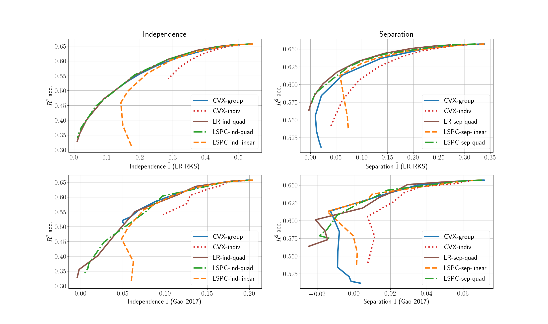
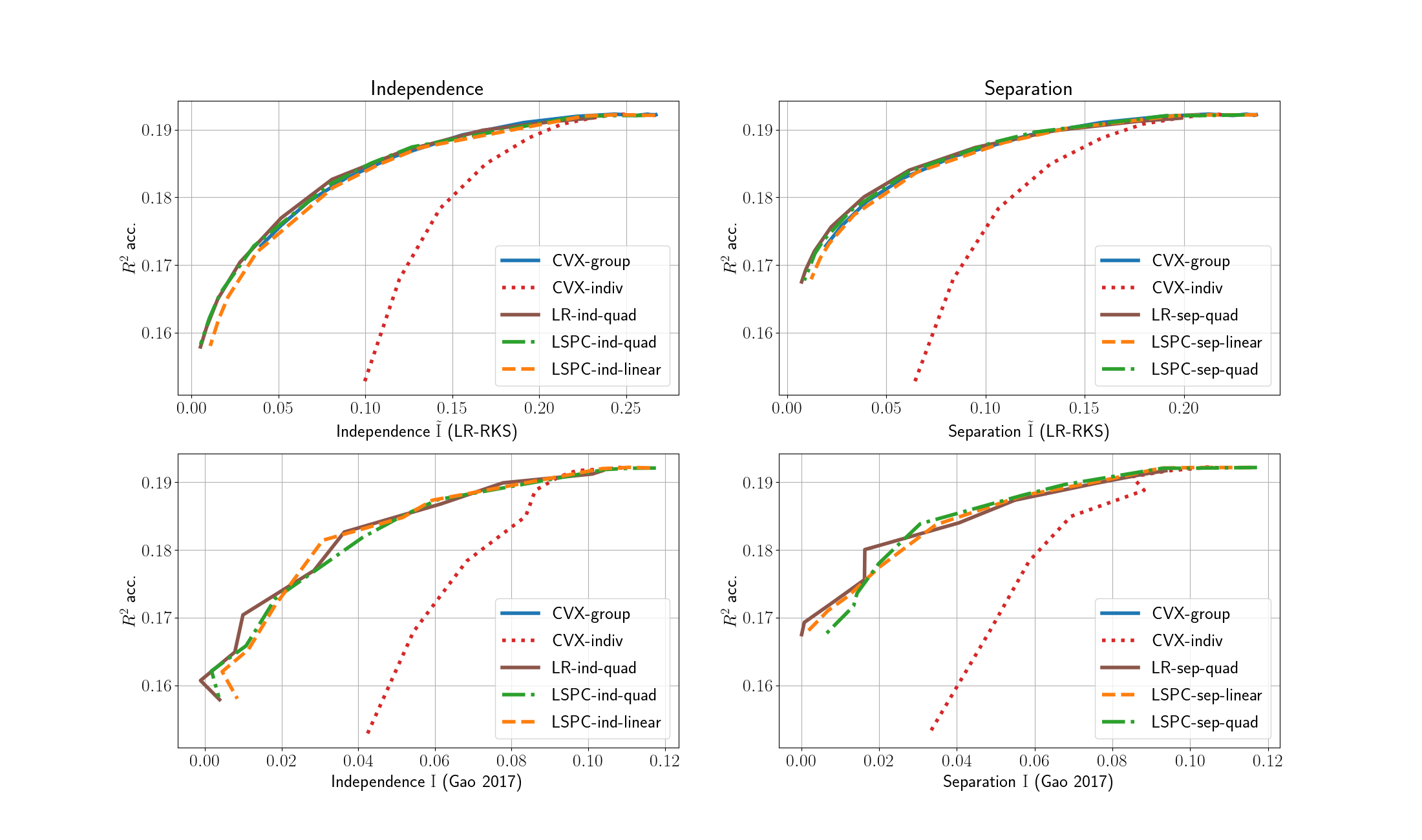
The efficiency results are summarised in Figures 1(a) and 1(b). We have not included the sufficiency results as predictions from the base linear models already satisfied this criterion, making the comparison uninformative.

In the CC results (Figure 1(a)) we can see that the LSPC regularisers with the quadratic (feature-cross) basis were the most efficient at satisfying the fairness criteria. The ‘group’ convex regulariser was also similarly efficient for some settings of the regulariser coefficients, though we could not get it to perfectly satisfy either independence or separation. This is to be expected because this regulariser does not encode these criteria exactly in its formulation. This is further demonstrated in its inflection away from satisfying separation for larger values of $\gamma$. The convex ‘individual’ regulariser also cannot satisfy these criteria for the same reason, though it seems to be encoding a fairness criterion quite dissimilar from either separation or independence. The linear version of LSPC does not perform well on this dataset at all, even though it is trying to satisfy these criteria. The reason for this behaviour is a systemic bias in its estimation of conditional entropy arising from its lower modelling capacity. In this case it pays off to take the (small) computational cost of the quadratic basis version of the LSPC approximation for and improved conditional entropy approximation.

In the LSAC dataset for the most part we can see similar performance to the CC dataset. The notable exception to this is now the linear LSPC regulariser has sufficient modelling capacity to (mostly) satisfy the separation and independence fairness criteria.

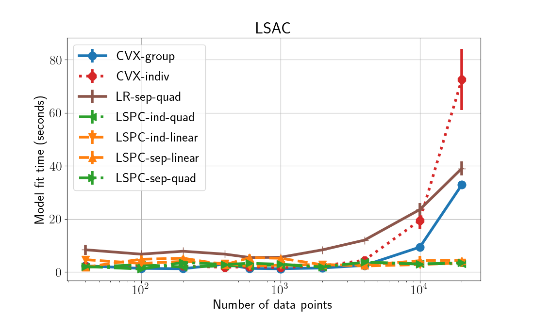
We also ran timing comparisons between the different regularisation methods, results shown in Figure 2. These results have been generated using increasing subset sizes of the LSAC dataset. The bars indicate the variation of time with respect to changing $\gamma$ — typically larger values were used so we emphasis the optimisation time of “fair” models. All other parameters were held constant. We believe these are good representations of performance since we implemented all methods, and used exactly the same base linear model code. These results are in-line with our expectations, as the (Berk et al., 2017) regularisers scale as $\mathcal{O}\!\left({n^{2}}\right)$, whereas our LSPC is simply a linear classifier, and so scales as $\mathcal{O}\!\left({n}\right)$.

We believe these results support our claims of LSPC being an efficient and effective means of approximating a conditional entropy based fairness regulariser. In the next experiment section we will further explore the efficacy of LSPC in approximating our normalised MI measures, $\tilde{\mathrm{I}}$.

5.2 Quality of Mutual Information Approximations

The fact that the accuracy$/$fairness trade-off curves of the proposed method are comparable to those of a state-of-the-art method suggests that our approximations to mutual information despite fast may be indeed reasonable. In this section we empirically investigate this hypothesis.

(a)

(b)

(c)

Figure 3: Comparison of MI estimators against the Monte Carlo approximation for a parameterised joint distribution.

Figure 4: Run time comparison of mutual information approximation methods.

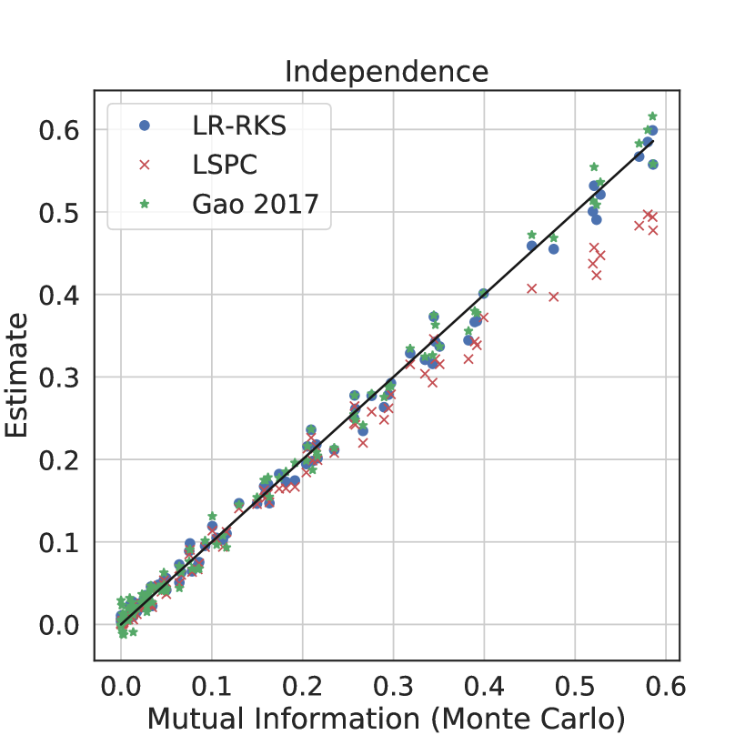
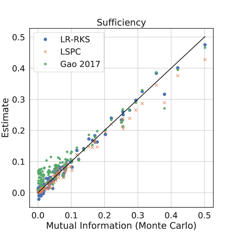
To estimate the accuracy of the proposed MI estimators, we created a parameterised joint probability distribution over $Y$, $S$ and $A$ in which the true mutual information could be independently quantified to a high precision using Monte Carlo integration. We used a Bernoulli distribution to model a binary sensitive attribute, $A$, which then conditioned a multivariate Gaussian distribution that represented the target values and regressor scores $Y$ and $S$, respectively.

Varying the mean and covariance of the conditional Gaussian distribution enabled us to generate joint distributions that exhibited potentially problematic characteristics from a fairness perspective. These include differences in base-rates, regressor accuracy and score across the protected classes.

Figure 3 illustrates the performance of each MI estimator when compared against the Monte Carlo approximation of mutual information over 100 different scenarios (the Monte Carlo approximation is our gold standard in this evaluation). LR-RKS and Gao 2017 are a logistic regressor with Fourier features (kitchen sinks) sinks (Rahimi & Recht, 2008) and the KSG estimator proposed in (Gao et al., 2017), respectively. These are used in §5.1 as independent estimates of MI because an analytical joint distribution was not available. LSPC refers to the our fast approximation of MI described in §4.3. We can see from the figure that the quality of our LSPC approximation is indeed reasonable — although not as good as for the most expensive methods. Further refining the quality of this approximation without significantly affecting its efficiency is left as a direction for future work.

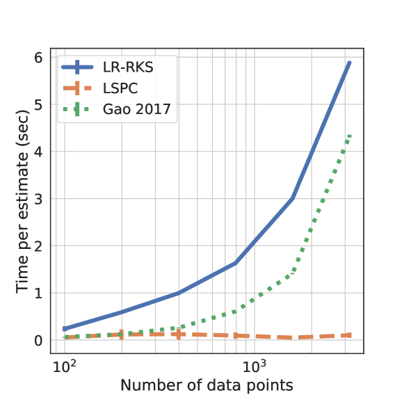
Fig. 4 shows that despite the fact that the quality of our mutual information approximation is similar to that of the other methods, its computational efficiency is significantly higher. This is the key justification behind the proposed approach.

6 Conclusion

In this paper we have studied the problem of learning a regression model under group fairness constraints as defined by the fairness criteria of independence, separation and sufficiency. Deviations from perfect alignment with each of these criteria can be quantified in terms of (conditional) mutual information, which motivates the use of these quantities as regularisers in order to trade-off accuracy and fairness in an regularised empirical risk minimisation framework. General approximations for mutual information can be computationally expensive, so we devised a fast approximation procedure particularly suited for the mixed categorical$/$continuous distributions arising due to protected classes being discrete and predicted outputs continuous. We have shown experimentally that the proposed approximation to mutual information, although much faster than alternatives, is not significantly less accurate. As a result, when we then incorporated these approximations as regularisers in a regression setting, we obtained comparable accuracy$/$fairness trade-offs to a state-of-the-art method — while being significantly more computationally efficient.

Appendix A Entropy Regularisers — Extended Results

The main paper proposes fairness regularisers promoting statistical separation, independence or sufficiency in a regression setting. The approach employs probabilistic classification to estimate conditional probabilities of the protected attributes.

This means that a classification model is nested inside the regression model’s training objective. The classifier’s trained predictive outputs, and their gradients, need to be efficiently computed at each step of the training optimisation for this approach to be computationally tractable.

For this purpose we employed the LSPC classifier, a least-squares approximation of a logistic regressor (Sugiyama et al., 2010; Sugiyama, 2010). In our application, this model closely approximates the performance of the same objective using a standard logistic regressor, while offering a faster closed form expression for the trained classifier’s predictive probabilities. Evidence of this statement was deferred to this supplementary material.

Here we include experimental results obtained using a standard logistic regression classifier inside our fairness regulariser. The logistic regression model is using the same quadratic feature expansion as our LSPC-quad implementations, and retrained at every evaluation of the regressor loss using nested numerical optimisation. Relevant regression objective gradients were inferred using knowledge that the classifier’s objective gradient was zero.

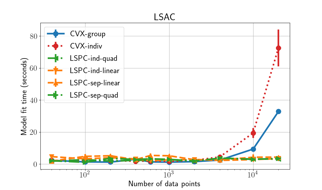
As shown in Figures 5(a) and 5(b), over our experimental datasets the LSPC-quad indeed offers equivalent predictive performance to the full logistic regressor that it approximates. On the other hand, the timing plots in Figure 6 show that the least squares approximation is significantly faster and scales better with respect to dataset size.

(a) Communities and Crime dataset.

(b) LSAC dataset.

Figure 5: Efficiency frontier, comparing our regulariser as proposed with a fast approximate classifier (LSPC) to our regulariser using a standard logistic regression model on the same features (LR). As detailed in the main paper, the CVX-group and CVX-indiv are the group and individual fairness regularisers proposed in Berk et al. (2017), and LSPC are our proposed implementation, with ‘ind’ and ‘sep’ denoting the independence and separation objectives, and ‘linear’ and ‘quad’ denoting a linear or feature-cross basis. The frontier is plotted in terms of $R^{2}$ accuracy, and Independence and Separation using normalised conditional mutual information (using both using probabilistic classification (LR-RKS), and mixed discrete-continuous MI estimation procedure of Gao et al. (2017) as detailed in the main paper).

Figure 6: Regressor training times as a function of the size of the training dataset using each fairness regressor. The proposed LSPC-sep-quad (employing a least squares probabilistic classifier) is a fast approximation of LR-sep-quad (employing a logistic regression classifier), and scales better with dataset size. The x-axis denotes the subset size of the LSAC dataset used to time the model fitting, and the bars depict the range of times for a sweep of regulariser strengths, $\gamma$.

References

- Agarwal et al. (2019) Agarwal, A., Dudik, M., and Wu, Z. S. Fair regression: Quantitative definitions and reduction-based algorithms. In Chaudhuri, K. and Salakhutdinov, R. (eds.), International Conference on Machine Learning, volume 97, pp. 120–129. PMLR, 2019.
- Angwin et al. (2016) Angwin, J., Larson, J., Mattu, S., and Kirchner, L. Machine bias. ProPublica, May 2016. URL https://www.propublica.org/article/machine-bias-risk-assessments-in-criminal-sentencing.
- Barocas et al. (2019) Barocas, S., Hardt, M., and Narayanan, A. Fairness and Machine Learning. fairmlbook.org, 2019. URL https://fairmlbook.org/.
- Belghazi et al. (2018) Belghazi, M. I., Baratin, A., Rajeshwar, S., Ozair, S., Bengio, Y., Courville, A., and Hjelm, D. Mutual information neural estimation. In International Conference on Machine Learning, pp. 531–540, 2018.
- Berk et al. (2017) Berk, R., Heidari, H., Jabbari, S., Joseph, M., Kearns, M., Morgenstern, J., Neel, S., and Roth, A. A convex framework for fair regression. Proceedings of the Conference on Fairness, Accountability, and Transparency - FAT* ’17, 2017.
- Byrd et al. (1995) Byrd, R. H., Lu, P., Nocedal, J., and Zhu, C. A limited memory algorithm for bound constrained optimization. SIAM Journal on scientific computing, 16(5):1190–1208, 1995.
- Calders et al. (2013) Calders, T., Karim, A., Kamiran, F., Ali, W., and Zhang, X. Controlling Attribute Effect in Linear Regression. In 2013 IEEE 13th International Conference on Data Mining, pp. 71–80, Dallas, TX, USA, December 2013. IEEE.
- Cleary (1968) Cleary, T. A. Test bias: Prediction of grades of negro and white students in integrated colleges. Journal of Educational Measurement, 5(2):115–124, 1968.
- Cover & Thomas (2006) Cover, T. M. and Thomas, J. A. Elements of information theory. John Wiley & Sons, 2nd edition, 2006.
- Darlington (1971) Darlington, R. B. Another look at “cultural fairness”. Journal of Educational Measurement, 8(2):71–82, 1971.
- Dua & Graff (2017) Dua, D. and Graff, C. UCI machine learning repository, 2017. URL http://archive.ics.uci.edu/ml.
- Fitzsimons et al. (2019) Fitzsimons, J., Ali, A. A., Osborne, M., and Roberts, S. A General Framework for Fair Regression. Entropy, 21(8):741, Jul 2019. ISSN 1099-4300.
- Fukuchi et al. (2015) Fukuchi, K., Kamishima, T., and Sakuma, J. Prediction with model-based neutrality. IEICE TRANSACTIONS on Information and Systems, 98(8):1503–1516, 2015.
- Gao et al. (2017) Gao, W., Kannan, S., Oh, S., and Viswanath, P. Estimating mutual information for discrete-continuous mixtures. In Advances in neural information processing systems, pp. 5986–5997, 2017.
- Gao et al. (2018) Gao, W., Oh, S., and Viswanath, P. Demystifying Fixed -Nearest Neighbor Information Estimators. IEEE Transactions on Information Theory, 64(8):5629–5661, 2018.
- Gel’fand & Yaglom (1957) Gel’fand, I. M. and Yaglom, A. M. Calculation of amount of information about a random function contained in another such function. American Mathematical Society Translations, 12:199–246, 1957. English translation of original in Uspekhi Matematicheskikh Nauk 12 (1): 3-52.
- Ghassami et al. (2018) Ghassami, A., Khodadadian, S., and Kiyavash, N. Fairness in supervised learning: An information theoretic approach. In 2018 IEEE International Symposium on Information Theory (ISIT), pp. 176–180. IEEE, 2018.
- Hastie et al. (2001) Hastie, T., Tibshirani, R., and Friedman, J. The elements of statistical learning, volume 1. Springer series in statistics New York, 2001.
- Hutchinson & Mitchell (2019) Hutchinson, B. and Mitchell, M. 50 Years of Test (Un)fairness: Lessons for Machine Learning. Proceedings of the Conference on Fairness, Accountability, and Transparency - FAT* ’19, pp. 49–58, 2019.
- Kamishima et al. (2012) Kamishima, T., Akaho, S., Asoh, H., and Sakuma, J. Fairness-Aware Classifier with Prejudice Remover Regularizer. In Machine Learning and Knowledge Discovery in Databases, volume 7524, pp. 35–50. Springer Berlin Heidelberg, Berlin, Heidelberg, 2012.
- Kanamori et al. (2010) Kanamori, T., Suzuki, T., and Sugiyama, M. Theoretical Analysis of Density Ratio Estimation. IEICE Transactions on Fundamentals of Electronics, Communications and Computer Sciences, E93-A(4):787–798, 2010.
- Komiyama et al. (2018) Komiyama, J., Takeda, A., Honda, J., and Shimao, H. Nonconvex Optimization for Regression with Fairness Constraints. In International conference on machine learning (ICML), pp. 2737–2746, 2018.
- Kraskov et al. (2004) Kraskov, A., Stögbauer, H., and Grassberger, P. Estimating mutual information. Physical review E, 69(6):066138, 2004.
- Rahimi & Recht (2008) Rahimi, A. and Recht, B. Random features for large-scale kernel machines. In Advances in neural information processing systems, pp. 1177–1184, 2008.
- Redmond & Baveja (2002) Redmond, M. and Baveja, A. A data-driven software tool for enabling cooperative information sharing among police departments. European Journal of Operational Research, 141(3):660–678, 2002.
- Sugiyama (2010) Sugiyama, M. Superfast-Trainable Multi-Class Probabilistic Classifier by Least-Squares Posterior Fitting. IEICE Transactions on Information and Systems, E93-D(10):2690–2701, 2010. ISSN 0916-8532, 1745-1361. doi: 10.1587/transinf.E93.D.2690.
- Sugiyama et al. (2010) Sugiyama, M., Hachiya, H., Simm, J., Yamada, M., and Nam, H. A computationally-efficient alternative to kernel logistic regression. In 2010 IEEE International Workshop on Machine Learning for Signal Processing, pp. 124–129, Kittila, Finland, August 2010. IEEE. ISBN 978-1-4244-7875-0. doi: 10.1109/MLSP.2010.5589255.
- Wightman (1998) Wightman, L. F. LSAC National Longitudinal Bar Passage Study. LSAC research report series. 1998.
- Williamson & Menon (2019) Williamson, R. and Menon, A. Fairness risk measures. In International Conference on Machine Learning, pp. 6786–6797, 2019.
- Zafar et al. (2015) Zafar, M. B., Valera, I., Rodriguez, M. G., and Gummadi, K. P. Fairness Constraints: Mechanisms for Fair Classification. arXiv:1507.05259 [cs, stat], July 2015.