Simple Interactive Image Segmentation using Label Propagation through kNN graphs

Abstract

Many interactive image segmentation techniques are based on semi-supervised learning. The user may label some pixels from each object and the SSL algorithm will propagate the labels from the labeled to the unlabeled pixels, finding object boundaries. This paper proposes a new SSL graph-based interactive image segmentation approach, using undirected and unweighted kNN graphs, from which the unlabeled nodes receive contributions from other nodes (either labeled or unlabeled). It is simpler than many other techniques, but it still achieves significant classification accuracy in the image segmentation task. Computer simulations are performed using some real-world images, extracted from the Microsoft GrabCut dataset. The segmentation results show the effectiveness of the proposed approach.

1 Introduction

Image segmentation is considered one of the most difficult tasks in image processing [Gonzalez and Woods 2008]. It is the process of dividing an image into parts, identifying objects or other relevant information [Shapiro and Stockman 2001]. Fully automatic segmentation is still very difficult to accomplish and the existing techniques are usually domain-dependent. Therefore, interactive image segmentation, in which the segmentation process is partially supervised, has experienced increasing interest in the last decades [Boykov and Jolly 2001, Grady 2006, Protiere and Sapiro 2007, Blake et al. 2004, Ducournau and Bretto 2014, Ding and Yilmaz 2010, Rother et al. 2004, Paiva and Tasdizen 2010, Li et al. 2010, Artan and Yetik 2010, Artan 2011, Xu et al. 2008, Breve et al. 2015b, Breve et al. 2015a].

Semi-supervised learning (SSL) is an important field in machine learning, usually applied when unlabeled data is abundant but the process of labeling is expensive, time consuming and/or requiring intensive work of human specialists [Zhu 2005, Chapelle et al. 2006]. This characteristics makes SSL an interesting approach to perform interactive image segmentation, which may be seen as a pixel classification process. In this scenario, there are often many unlabeled pixels to be classified. An human specialist can easily classify some of them, which are away from the borders, but the process of defining the borders manually is difficult and time consuming.

Many interactive image segmentation techniques are, in fact, based on semi-supervised learning. The user may label some pixels from each object, away from the boundaries where the task is easier. Then, the SSL algorithm will iteratively propagate the labels from the labeled pixels to the unlabeled pixels, finding the boundaries. This paper proposes a different SSL-based interactive image segmentation approach. It is simpler than many other techniques, but it still achieves significant classification accuracy in the image segmentation task. In particular, it was applied to some real-world images, including some images extracted from the Microsoft GrabCut dataset [Rother et al. 2004]. The segmentation results show the effectiveness of the proposed approach.

1.1 Related work

The approach proposed in this paper may be classified in the category of graph-based semi-supervised learning. Algorithms on this category rely on the idea of building a graph which nodes are data items (both labeled and unlabeled) and the edges represent similarities between them. Label information from the labeled nodes is propagate through the graph to classify all the nodes [Chapelle et al. 2006]. Many graph-based methods [Blum and Chawla 2001, Zhu et al. 2003, Zhou et al. 2004, Belkin et al. 2004, Belkin et al. 2005, Joachims 2003] are similar and share the same regularization framework [Zhu 2005]. They usually employ weighted graphs and labels are spread globally, differently from the proposed approach, where the label spreading is limited to neighboring nodes and the graph is undirected and unweighted.

Another graph-based method, known as Label Propagation through Linear Neighborhoods [Wang and Zhang 2008], also uses a $k$-nearest neighbors graph to propagate labels. However, the edges have weights, which require the resolution of quadratic programming problems to be calculated, prior to the iterative label propagation process. On the other hand, the proposed approach uses only unweighted edges.

1.2 Technique overview

In the proposed method, an unweighted and undirected graph is generated by connecting each node (data item) to its $k$-nearest neighbors. Then, in a iterative process, unlabeled nodes will receive contributions from all its neighbors (either labeled or unlabeled) to define their own label. The algorithm usually converges quickly, and each unlabeled node is labeled after the class from which it received most contributions. Differently from many other graph-based methods, no calculation of edge weights or Laplacian matrix are required.

2 The Proposed Model

In this section, the proposed technique will be detailed. Given a bidimensional digital image, the set of pixels are reorganized as $\mathfrak{X}=\{x_{1},x_{2},\dots,x_{L},x_{L+1},\dots,x_{N}\}$, such that $\mathfrak{X}_{L}=\{x_{i}\}_{i=1}^{L}$ is the labeled pixel subset and $\mathfrak{X}_{U}=\{x_{i}\}_{i=L+1}^{N}$ is the unlabeled pixels subset. $\mathfrak{L}=\{1,\dots,C\}$ is the set containing the labels. $y:\mathfrak{X}\rightarrow\mathfrak{L}$ is the function associating each $x_{i}\in\mathbf{\chi}$ to its label $y(x_{i})$ as the algorithm output. The algorithm will estimate $y(x_{i})$ for each unlabeled pixel $x_{i}\in\mathfrak{X}_{U}$.

2.1 $k$-NN Graph Generation

A large amount of features may be extracted from each pixel $x_{i}$ to build the graph. In this paper, $23$ features are used. They are shown on Table 1. These are the same features used in [Breve 2015].

Table 1: List of features extracted from each image to be segmented

#	Feature Description
1	Pixel row location
2	Pixel column location
3	Red (R) component of the pixel
4	Green (G) component of the pixel
5	Blue (B) component of the pixel
6	Hue (H) component of the pixel
7	Saturation (S) component of the pixel
8	Value (V) component of the pixel
9	ExR component of the pixel
10	ExG component of the pixel
11	ExB component of the pixel
12	Average of R on the pixel and its neighbors (MR)
13	Average of G on the pixel and its neighbors (MG)
14	Average of B on the pixel and its neighbors (MB)
15	Standard deviation of R on the pixel and its neighbors (SDR)
16	Standard deviation of G on the pixel and its neighbors (SDG)
17	Standard deviation of B on the pixel and its neighbors (SDB)
18	Average of H on the pixel and its neighbors (MH)
19	Average of S on the pixel and its neighbors (MS)
20	Average of V on the pixel and its neighbors (MV)
21	Standard deviation of H on the pixel and its neighbors (SDH)
22	Standard deviation of S on the pixel and its neighbors (SDS)
23	Standard deviation of V on the pixel and its neighbors (SDV)

For measures $12$ to $23$, the pixel neighbors are the $8$-connected neighborhood, except on the borders where no wraparound is applied. All components are normalized to have mean $0$ and standard deviation $1$. They are also scaled by a vector of weights $\lambda$ in order to emphasize/deemphasize each feature during the graph generation. ExR, ExG, and ExB components are obtained from the RGB components using the method described in [Lichman 2013]. The HSV components are obtained from the RGB components using the method described in [Smith 1978].

The undirected and unweighted graph is defined as $\mathbf{G}=(\mathbf{V},\mathbf{E})$, where $\mathbf{V}=\{v_{1},v_{2},\dots,v_{N}\}$ is the set of nodes, and $\mathbf{E}$ is the set of edges $(v_{i},v_{j})$. Each node $v_{i}$ corresponds to a pixel $x_{i}$. Two nodes $v_{i}$ and $v_{j}$ are connected if $v_{j}$ is among the $k$-nearest neighbors of $v_{i}$, or vice-versa, considering the Euclidean distance between $x_{i}$ and $x_{j}$ features. Otherwise, $v_{i}$ and $v_{j}$ are disconnected.

2.2 Label Propagation

For each node $v_{i}$, a domination vector $\mathbf{v_{i}^{\omega}(t)}=\{v_{i}^{\omega_{1}}(t),v_{i}^{\omega_{2}}(t),\dots,v_{i}^{\omega_{C}}(t)\}$ is created. Each element $v_{i}^{\omega_{c}}(t)\in[0,1]$ corresponds to the domination level from the class $c$ over the node $v_{i}$. The sum of the domination vector in each node is always constant, $\sum_{c=1}^{C}v_{i}^{\omega_{c}}=1$.

The domination levels are constant in nodes corresponding to labeled pixels, with full domination by the corresponding class. On the other hand, domination levels are variable in nodes corresponding to unlabeled pixels and they are initially set equally among classes. Therefore, for each node $v_{i}$, the domination vector $\mathbf{v_{i}^{\omega}}$ is set as follows:

$$v_{i}^{\omega_{c}}(0)=\left\{\begin{array}[]{ccl}1&&\mbox{if $x_{i}$ is labeled and $y(x_{i})=c$}\\ 0&&\mbox{if $x_{i}$ is labeled and $y(x_{i})\neq c$}\\ \frac{1}{C}&&\mbox{if $x_{i}$ is unlabeled}\end{array}\right..$$ (1)

In the iterative phase, at each iteration each unlabeled node will get contributions from all its neighbors to calculate its new domination levels. Thus, for each unlabeled node $v_{i}$, the domination levels are updated as follows:

$$\mathbf{v_{i}^{\omega}(t+1)}=\frac{1}{K}\sum_{j\in N(v_{i})}\mathbf{v_{j}^{\omega}(t)},$$ (2)

where $K=|N(v_{i})|$ is the size of $N(v_{i})$, and $N(v_{i})$ is the set of the $v_{i}$ neighbors. In this way, the new dominance vector $\mathbf{v_{i}^{\omega}}$ is the arithmetic mean of all its neighbors dominance vectors, no matter if they are labeled or unlabeled.

The average maximum domination levels is defined as follows:

$$\langle v_{i}^{\omega_{m}}\rangle,m=\arg\max_{c}v_{i}^{\omega_{c}},$$ (3)

considering all $v_{i}$ representing unlabeled nodes. $\langle v_{i}^{\omega_{m}}\rangle$ is checked every $10$ iterations and the algorithm stops when its increase is below $0.001$ between checkpoints.

At the end of the iterative process, each unlabeled pixel is assigned to the class that has the highest domination level on it:

$$y(x_{i})=\arg\max_{c}v_{i}^{\omega_{c}}$$ (4)

2.3 The Algorithm

Overall, the proposed algorithm can be outlined as follows:

1 Build the $k$-NN graph, as described in Subsection 2.1;

2 Set nodes’ domination levels by using Eq. (1);

3 repeat

4       for each unlabeled node do

5             Update node domination levels by using Eq. (2);

6            

7      

8until the stopping criterion is satisfied;

Label each unlabeled pixel using Eq. (4);

Algorithm 1 The proposed method algorithm

3 Implementation

In order to reduce the computational resources required by the proposed method, the following implementation strategy is applied.

The iterative step of the algorithm is very fast in comparison with the graph generation step, i.e., the graph generation dominates the execution time. Therefore, the graph is generated using the k-d trees method [Friedman et al. 1977], so the algorithm runs in linearithmic time ($O(N\log N)$).

In the iterative step, each iteration runs in $O(uk)$, where $u$ is the amount of unlabeled nodes and $k$ is usually proportional to the amount of neighbors each node has (not equal because the graph is undirected). $u$ is usually a fraction of $N$ in practical problems, and often $k\ll n$. By increasing $k$, one also increases each iteration execution time. On the other hand, the amount of iterations required to converge decreases as the graph becomes more connected and the labels propagate faster, as it was empirically observed in computer simulations.

The iterative steps are synchronous, i.e., the contributions any node receives to produce its domination vector in time $t+1$ refer to the domination levels its neighbors had in time $t$. Therefore, parallelization of this step, corresponding to the inner loop in steps $4$ and $5$ of the Algorithm 1, is possible. Nodes can calculate their new domination vectors in parallel without running into race conditions. Synchronization is only required between iterations of the outer loop (steps $3$ to $6$).

4 Experiments

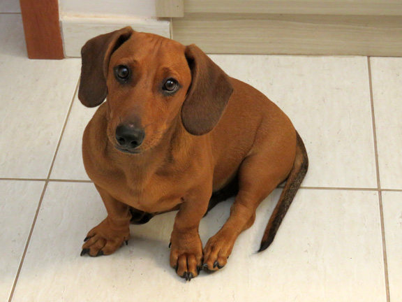
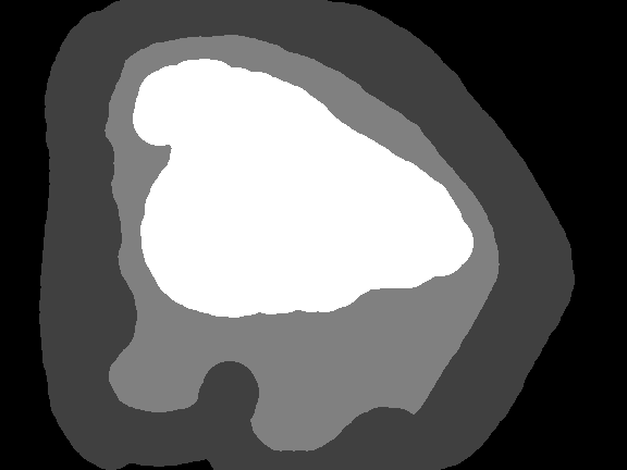
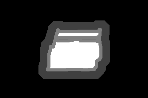
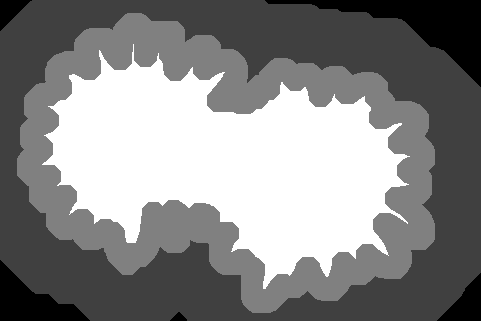
The proposed technique efficacy is first tested using the real-world image shown on Fig. 1a, extracted from [Breve et al. 2015b], which has $576\times 432$ pixels. A trimap providing seed regions is presented in Figure 1b. Black (0) represents the background, ignored by the algorithm; dark gray (64) is the labeled background; light gray (128) is the unlabeled region, which labels will be estimated by the proposed method; and white (255) is the labeled foreground.

(a)

(b)

(c)

Figure 1: (a) Original image, (b) Trimap providing seed regions for Fig. 1a segmentation, (c) Close-up foreground segmentation results by the proposed method.

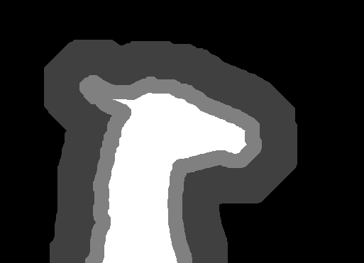
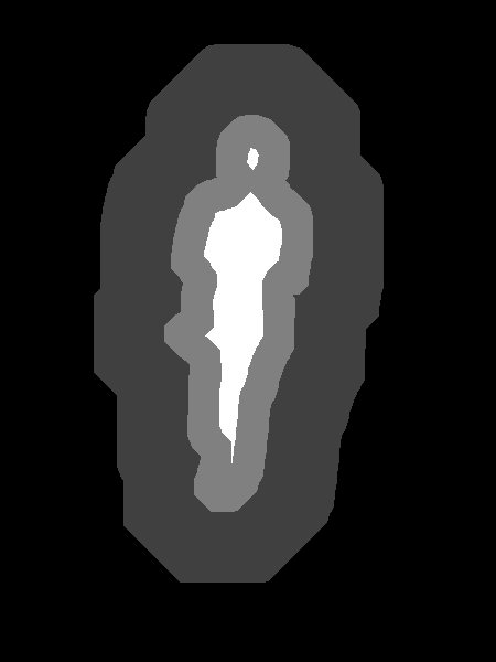
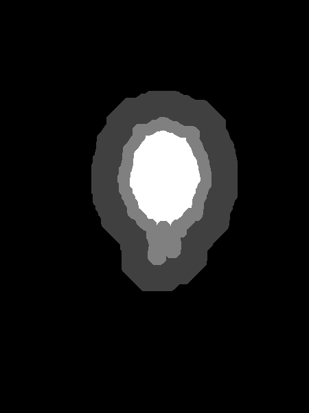
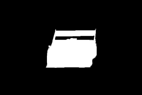
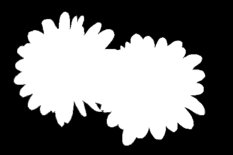
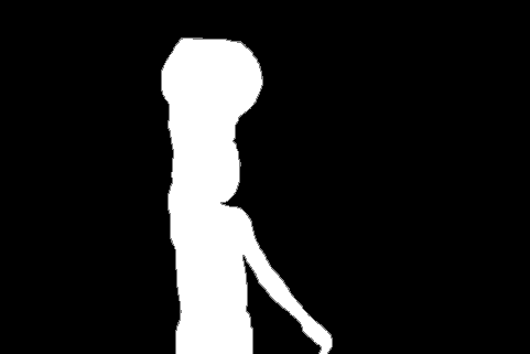
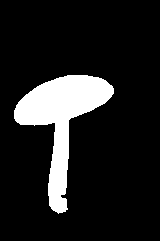
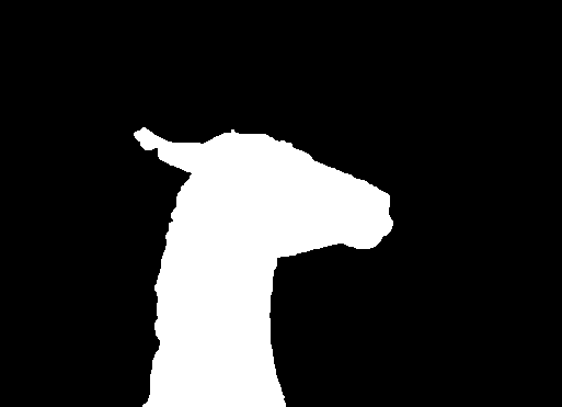
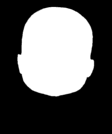
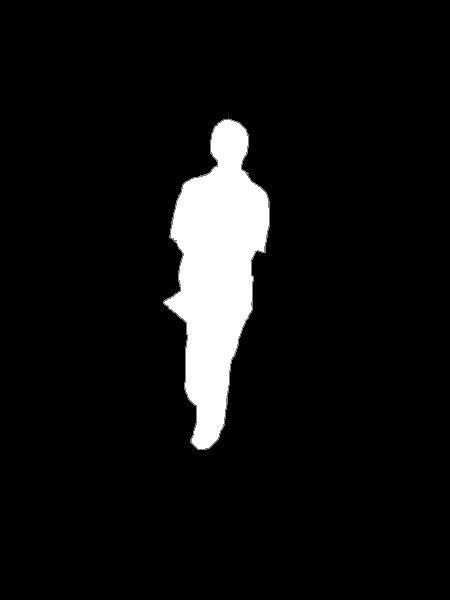
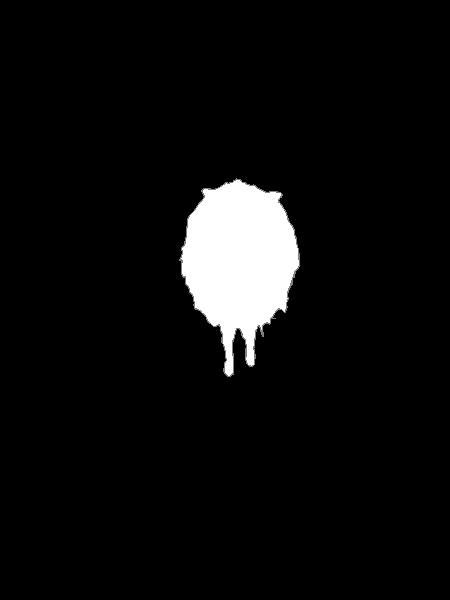
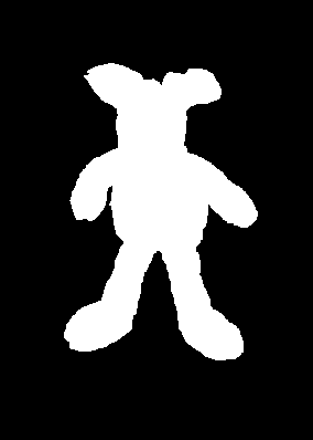
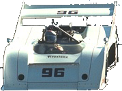
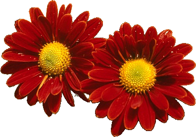
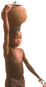
The proposed technique efficacy is then verified using a series of computational experiments using nine image selected from the Microsoft GrabCut database [Rother et al. 2004] . The selected images are shown on Fig. 2. The corresponding trimaps providing seed regions are shown on Fig. 3. Finally, the ground truth images are shown on Fig. 4.

(a)

(b)

(c)

(d)

(e)

(f)

(g)

(h)

(i)

Figure 2: Original images from the GrabCut dataset: (a) 21077; (b) 124084; (c) 271008; (d) 208001; (e) llama; (f) doll; (g) person7; (h) sheep; (i) teddy.

(a)

(b)

(c)

(d)

(e)

(f)

(g)

(h)

(i)

Figure 3: The trimaps providing seed regions from the GrabCut dataset: (a) 21077; (b) 124084; (c) 271008; (d) 208001; (e) llama; (f) doll; (g) person7; (h) sheep; (i) teddy.

(a)

(b)

(c)

(d)

(e)

(f)

(g)

(h)

(i)

Figure 4: Close-up foreground segmentation results by the proposed method: (a) 21077; (b) 124084; (c) 271008; (d) 208001; (e) llama; (f) doll; (g) person7; (h) sheep; (i) teddy.

For each image, $k$ and the vector of weights $\lambda$ were optimized using the genetic algorithm available in Global Optimization Toolbox of MATLAB, with its default parameters.

5 Results and Discussion

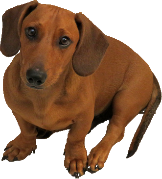
First, the proposed method was applied to the image shown on Fig. 1a. The best segmentation result is shown on Fig. 1c. By comparing this output with the segmentation result achieved in [Breve et al. 2015b] for the same image, one can notice that the proposed method achieved slightly better results, by eliminating some misclassified pixels and better defining the borders.

Then, the proposed method was applied to the nine images shown on Fig. 2, as described on Section 4. The best segmentation results achieved with the proposed method are shown on Fig. 5. Error rates are computed as the fraction between the amount of incorrectly classified pixels and the total amount of unlabeled pixels (light gray on the trimaps images shown on Fig. 3). Notice that ground truth images (Fig. 4) have a thin contour of gray pixels, which corresponds to uncertainty, i.e., pixels that received different labels by the different persons who did the manual classification. These pixels are not used in the classification error calculation.

(a) 5.13%

(b) 0.57%

(c) 3.09%

(d) 3.88%

(e) 6.83%

(f) 0.64%

(g) 1.09%

(h) 1.41%

(i) 1.63%

Figure 5: The ground-truth images from the GrabCut dataset: (a) 21077; (b) 124084; (c) 271008; (d) 208001; (e) llama; (f) doll; (g) person7; (h) sheep; (i) teddy. Error rates are indicated below each image.

Segmentation error rates are also summarized on Table 2. Some results from other methods [Ducournau and Bretto 2014, Ding and Yilmaz 2008, Breve et al. 2015b] are also included for reference. By analyzing them, one can notice that the proposed method has comparable results. The results from the other methods were extracted from the respective references.

Table 2: Segmentation error rates achieved by Learning on Hypergraphs model (ISLH) [Ding and Yilmaz 2008], Directed Image Neighborhood Hypergraph model (DINH) [Ducournau and Bretto 2014], Particle Competition and Cooperation (PCC) [Breve et al. 2015b] and the proposed model (LPKNN).

It is also important to notice that the proposed method is deterministic. Given the same parameters, it will always output the same segmentation result on different executions. Other methods, like Particle Competition and Cooperation [Breve et al. 2015b], are stochastic. Therefore, they may output different segmentation results on each execution.

The optimized parameters $k$ and features weights ($\lambda$) are shown on Table 3. Considering the $10$ images evaluated in this paper, pixel location features (Row and Col) are the most important features, followed by the ExB component, intensity (V), and the mean of green (MG). The least important features were hue (H), saturation (S) and all those related to standard deviation. However, no single feature received a high weight in all images. The optimal weights and $k$ seem to be highly dependent on image characteristics.

Table 3: Parameter $k$ and feature weights $\lambda$ optimized by the proposed method for each segmented image.

6 Conclusion

In this paper, a new SSL graph-based approach is proposed to perform interactive image segmentation. It employs undirected and unweighted $k$NN graphs to propagate labels from nodes representing labeled pixels to nodes representing unlabeled pixels. Computer simulations with some real-world images show that the proposed approach is effective, achieving segmentation accuracy similar to those achieved by some state-of-the-art methods.

As future work, the method will be applied on more images and more features may be extracted. Methods to automatically define the parameters $k$ and $\lambda$ may also be explored. Graph generation may also be improved to provide further increase in segmentation accuracy.

Moreover, the proposed method works for multiple labels simultaneously at no extra cost, which is an interesting property not often exhibited by other interactive image segmentation methods. This feature will also be explored in future works.

References

- [Artan 2011] Artan, Y. (2011). Interactive image segmentation using machine learning techniques. In Computer and Robot Vision (CRV), 2011 Canadian Conference on, pages 264–269.
- [Artan and Yetik 2010] Artan, Y. and Yetik, I. (2010). Improved random walker algorithm for image segmentation. In Image Analysis Interpretation (SSIAI), 2010 IEEE Southwest Symposium on, pages 89–92.
- [Belkin et al. 2004] Belkin, M., Matveeva, I., and Niyogi, P. (2004). Regularization and semisupervised learning on large graphs. In Conference on Learning Theory, pages 624–638. Springer.
- [Belkin et al. 2005] Belkin, M., P., N., and Sindhwani, V. (2005). On manifold regularization. In Proceedings of the Tenth International Workshop on Artificial Intelligence and Statistics (AISTAT 2005), pages 17–24, New Jersey. Society for Artificial Intelligence and Statistics.
- [Blake et al. 2004] Blake, A., Rother, C., Brown, M., Perez, P., and Torr, P. (2004). Interactive image segmentation using an adaptive gmmrf model. In Pajdla, T. and Matas, J., editors, Computer Vision - ECCV 2004, volume 3021 of Lecture Notes in Computer Science, pages 428–441. Springer Berlin Heidelberg.
- [Blum and Chawla 2001] Blum, A. and Chawla, S. (2001). Learning from labeled and unlabeled data using graph mincuts. In Proceedings of the Eighteenth International Conference on Machine Learning, pages 19–26, San Francisco. Morgan Kaufmann.
- [Boykov and Jolly 2001] Boykov, Y. and Jolly, M.-P. (2001). Interactive graph cuts for optimal boundary amp; region segmentation of objects in n-d images. In Computer Vision, 2001. ICCV 2001. Proceedings. Eighth IEEE International Conference on, volume 1, pages 105–112 vol.1.
- [Breve et al. 2015a] Breve, F., Quiles, M., and Zhao, L. (2015a). Interactive image segmentation of non-contiguous classes using particle competition and cooperation. In Gervasi, O., Murgante, B., Misra, S., Gavrilova, M. L., Rocha, A. M. A. C., Torre, C., Taniar, D., and Apduhan, B. O., editors, Computational Science and Its Applications – ICCSA 2015, volume 9155 of Lecture Notes in Computer Science, pages 203–216. Springer International Publishing.
- [Breve et al. 2015b] Breve, F., Quiles, M. G., and Zhao, L. (2015b). Interactive image segmentation using particle competition and cooperation. In 2015 International Joint Conference on Neural Networks (IJCNN), pages 1–8.
- [Breve 2015] Breve, F. A. (2015). Auto feature weight for interactive image segmentation using particle competition and cooperation. In Proceedings - XI Workshop de Visão Computacional WVC’2015, pages 164–169.
- [Chapelle et al. 2006] Chapelle, O., Schölkopf, B., and Zien, A., editors (2006). Semi-Supervised Learning. Adaptive Computation and Machine Learning. The MIT Press, Cambridge, MA.
- [Ding and Yilmaz 2008] Ding, L. and Yilmaz, A. (2008). Image segmentation as learning on hypergraphs. In Machine Learning and Applications, 2008. ICMLA ’08. Seventh International Conference on, pages 247–252.
- [Ding and Yilmaz 2010] Ding, L. and Yilmaz, A. (2010). Interactive image segmentation using probabilistic hypergraphs. Pattern Recognition, 43(5):1863 – 1873.
- [Ducournau and Bretto 2014] Ducournau, A. and Bretto, A. (2014). Random walks in directed hypergraphs and application to semi-supervised image segmentation. Computer Vision and Image Understanding, 120(0):91 – 102.
- [Friedman et al. 1977] Friedman, J. H., Bentley, J. L., and Finkel, R. A. (1977). An algorithm for finding best matches in logarithmic expected time. ACM Trans. Math. Softw., 3(3):209–226.
- [Gonzalez and Woods 2008] Gonzalez, R. C. and Woods, R. E. (2008). Digital Image Processing (3rd Edition). Prentice-Hall, Inc., Upper Saddle River, NJ, USA.
- [Grady 2006] Grady, L. (2006). Random walks for image segmentation. Pattern Analysis and Machine Intelligence, IEEE Transactions on, 28(11):1768–1783.
- [Joachims 2003] Joachims, T. (2003). Transductive learning via spectral graph partitioning. In Proceedings of International Conference on Machine Learning, pages 290–297. AAAI Press.
- [Li et al. 2010] Li, J., Bioucas-Dias, J., and Plaza, A. (2010). Semisupervised hyperspectral image segmentation using multinomial logistic regression with active learning. Geoscience and Remote Sensing, IEEE Transactions on, 48(11):4085–4098.
- [Lichman 2013] Lichman, M. (2013). UCI machine learning repository.
- [Paiva and Tasdizen 2010] Paiva, A. and Tasdizen, T. (2010). Fast semi-supervised image segmentation by novelty selection. In Acoustics Speech and Signal Processing (ICASSP), 2010 IEEE International Conference on, pages 1054–1057.
- [Protiere and Sapiro 2007] Protiere, A. and Sapiro, G. (2007). Interactive image segmentation via adaptive weighted distances. Image Processing, IEEE Transactions on, 16(4):1046–1057.
- [Rother et al. 2004] Rother, C., Kolmogorov, V., and Blake, A. (2004). “grabcut”: Interactive foreground extraction using iterated graph cuts. ACM Trans. Graph., 23(3):309–314.
- [Shapiro and Stockman 2001] Shapiro, L. and Stockman, G. (2001). Computer Vision. Prentice Hall.
- [Smith 1978] Smith, A. R. (1978). Color gamut transform pairs. In ACM Siggraph Computer Graphics, volume 12, pages 12–19. ACM.
- [Wang and Zhang 2008] Wang, F. and Zhang, C. (2008). Label propagation through linear neighborhoods. IEEE Transactions on Knowledge and Data Engineering, 20(1):55–67.
- [Xu et al. 2008] Xu, J., Chen, X., and Huang, X. (2008). Interactive image segmentation by semi-supervised learning ensemble. In Knowledge Acquisition and Modeling, 2008. KAM ’08. International Symposium on, pages 645–648.
- [Zhou et al. 2004] Zhou, D., Bousquet, O., Lal, T. N., Weston, J., and Schölkopf, B. (2004). Learning with local and global consistency. In Advances in Neural Information Processing Systems, volume 16, pages 321–328. MIT Press.
- [Zhu 2005] Zhu, X. (2005). Semi-supervised learning literature survey. Technical Report 1530, Computer Sciences, University of Wisconsin-Madison.
- [Zhu et al. 2003] Zhu, X., Ghahramani, Z., and Lafferty, J. (2003). Semi-supervised learning using gaussian fields and harmonic functions. In Proceedings of the Twentieth International Conference on Machine Learning, pages 912–919.