Sequential Cooperative Bayesian Inference

Junqi Wang    Pei Wang    Patrick Shafto
Abstract

Cooperation is often implicitly assumed when learning from other agents. Cooperation implies that the agent selecting the data, and the agent learning from the data, have the same goal, that the learner infer the intended hypothesis. Recent models in human and machine learning have demonstrated the possibility of cooperation. We seek foundational theoretical results for cooperative inference by Bayesian agents through sequential data. We develop novel approaches analyzing consistency, rate of convergence and stability of Sequential Cooperative Bayesian Inference (SCBI). Our analysis of the effectiveness, sample efficiency and robustness show that cooperation is not only possible in specific instances but theoretically well-founded in general. We discuss implications for human-human and human-machine cooperation.

Bayesian inference, cooperative inference, multi-agent learning, Machine Learning, ICML

1 Introduction

Learning often occurs sequentially, as opposed to in batch, and from data provided by other agents, as opposed to from a fixed random sampling process. The canonical example of sequential learning from an agent occurs in educational contexts where the other agent is a teacher whose goal is to help the learner. However, instances appear across a wide range of contexts including informal learning, language, and robotics. In contrast with typical contexts considered in machine learning, it is reasonable to expect the cooperative agent to adapt their sampling process after each trial, consistent with the goal of helping the learner learn more quickly. It is also reasonable to expect that learners, in dealing with such cooperative agents, would know the other agent intends to cooperate and incorporate that knowledge when updating their beliefs. In this paper, we analyze basic statistical properties of such sequential cooperative inferences.

Large behavioral and computational literatures highlight the importance cooperation for learning. Across behavioral sciences, cooperative information sharing is believed to be a core feature of human cognition. Education, where a teacher selects examples for a learner, is perhaps the most obvious case. Other examples appear in linguistic pragmatics (Frank & Goodman, 2012), in speech directed to infants (Eaves Jr et al., 2016), and children’s learning from demonstrations (Bonawitz et al., 2011). Indeed, theorists have posited that the ability to select data for and learn cooperatively from others explains humans’ ability to learning quickly in childhood and accumulate knowledge over generations (Tomasello, 1999; Csibra & Gergely, 2009).

Across computational literatures, cooperative information sharing is also believed to be central to human-machine interaction. Examples include pedagogic-pragmatic value alignment in robotics (Fisac et al., 2017), cooperative inverse reinforcement learning (Hadfield-Menell et al., 2016), machine teaching (Zhu, 2013), and Bayesian teaching (Eaves Jr et al., 2016) in machine learning, and Teaching dimension in learning theory (Zilles et al., 2008; Doliwa et al., 2014). Indeed, rather than building in knowledge or training on massive amounts of data, cooperative learning from humans is a strong candidate for advancing machine learning theory and improving human-machine teaming more generally.

While behavioral and computational research makes clear the importance of cooperation for learning, we lack mathematical results that would establish statistical soundness. In the development of probability theory, proofs of consistency and rate of convergence were celebrated results that put Bayesian inference on strong mathematical footing (Doob, 1949). Moreover, establishment of stability with respect to mis-specification ensured that theoretical results could apply despite the small differences between the model and reality (Kadane et al., 1978; Berger et al., 1994). Proofs of consistency, convergence, and stability ensure that intuitions regarding probabilistic inference were formalized in ways that satisfied basic desiderata.

Our goal is to provide a comparable foundation for sequential Cooperative Bayesian Inference as statistical inference for understanding the strengths, limitations, and behavior of cooperating agents. Grounded strongly in machine learning (Murphy, 2012; Ghahramani, 2015) and human learning (Tenenbaum et al., 2011), we adopt a probabilistic approach. We approach consistency, convergence, and stability using a combination of new analytical and empirical methods. The result will be a model agnostic understanding of whether and under what conditions sequential cooperative interactions result in effective and efficient learning.

Notations are introduced at the end of this section. Section 2 introduces the model of sequential cooperative Bayesian inference (SCBI), and Bayesian inference (BI) as the comparison. Section 3 presents a new analysis approach which we apply to understanding consistency of SCBI. Section 4 presents empirical results analyzing the sample efficiency of SCBI versus BI, showing convergence of SCBI is considerably faster. Section 5 presents the empirical results testing robustness of SCBI to perturbations. Section 6 introduces an application of SCBI in Grid world model. Section 7 describes our contributions in the context of related work, and Section 8 discusses implications for machine learning and human learning.

Preliminaries. Throughout this paper, for a vector θ𝜃\theta, we denote its i𝑖i-th entry by θisubscript𝜃𝑖\theta_{i} or θ(i)𝜃𝑖\theta(i). Similarly, for a matrix 𝐌𝐌\mathbf{M}, we denote the vector of i𝑖i-th row by 𝐌(i,_)subscript𝐌𝑖_\mathbf{{M}}_{(i,\_)}, the vector of j𝑗j-th column by 𝐌(_,j)subscript𝐌_𝑗\mathbf{{M}}_{(\_,j)}, and the entry of i𝑖i-th row and j𝑗j-th column by 𝐌(i,j)subscript𝐌𝑖𝑗\mathbf{M}_{(i,j)} or simply 𝐌ijsubscript𝐌𝑖𝑗\mathbf{M}_{ij}. Further, let 𝐫,𝐜𝐫𝐜\mathbf{r},\mathbf{c} be the column vectors representing the row and column marginals (sums along row/column) of 𝐌𝐌\mathbf{M}. Let 𝐞nsubscript𝐞𝑛\mathbf{e}_{n} or simply 𝐞𝐞\mathbf{e} be the vector of ones. The symbol 𝒩vec(θ,s)subscript𝒩vec𝜃𝑠\mathscr{N}_{\text{vec}}\left(\theta,s\right) is used to denote the normalization of a non-negative vector θ𝜃\theta, i.e., 𝒩vec(θ,s)=sθiθsubscript𝒩vec𝜃𝑠𝑠subscript𝜃𝑖𝜃\mathscr{N}_{\text{vec}}\left(\theta,s\right)=\frac{s}{\sum\theta_{i}}\theta with s=1𝑠1s=1 if absent. Similarly, the normalization of matrices are denoted by 𝒩col(𝐌,θ)subscript𝒩col𝐌𝜃\mathscr{N}_{\text{col}}\left(\mathbf{M},\theta\right), with “col” indicating column normalization (for row normalization, write “row” instead), and θ𝜃\theta denotes to which vector of sums the matrix is normalized. The set of probability distributions on a finite set 𝒳𝒳\mathcal{X} is denoted by 𝒫(𝒳)𝒫𝒳\mathcal{P}(\mathcal{X}), we do not distinguish it with the simplex Δ|𝒳|1superscriptΔ𝒳1\Delta^{|\mathcal{X}|-1}. The language of statistical models and estimators follows the notations of the book (Miescke & Liese, 2008).

2 The Construction

hh𝐓𝐓\mathbf{T}\mathcal{H}𝒟𝒟\mathcal{D}θ0subscript𝜃0\theta_{0}𝐋𝐋\mathbf{L}TeacherLearner
Figure 1: Two agents and their knowledge before starting.

In this paper, we consider cooperative communication models with two agents, which we call a teacher and a learner. Let ={1,,m}1𝑚\mathcal{H}=\{1,\dots,m\} be the set of m𝑚m hypotheses, i.e., concepts to teach. The shared goal is for the learner to infer the correct hypothesis hh\in\mathcal{H} which is only known by the teacher at the beginning. To facilitate learning, the teacher passes one element from a finite data set 𝒟={1,,n}𝒟1𝑛\mathcal{D}=\{1,\dots,n\} sequentially. Each agent has knowledge about the relation between \mathcal{H} and 𝒟𝒟\mathcal{D}, in terms of a positive matrix whose normalization can be treated as the likelihood matrix in a Bayesian sense. Let 𝐓,𝐋Matn×m(+)𝐓𝐋subscriptMat𝑛𝑚superscript\mathbf{T},\mathbf{L}\in\mathrm{Mat}_{n\times m}(\mathbb{R}^{+}) be the matrices for teacher and learner, respectively.

In order to construct a Bayesian theory, the learner has an initial prior θ0subscript𝜃0\theta_{0} on \mathcal{H}, which, along with posteriors θk(k1)subscript𝜃𝑘𝑘1\theta_{k}(k\geq 1), are elements in 𝒫()=Δm1:={θm:i=1mθ(i)=1}𝒫superscriptΔ𝑚1assignconditional-set𝜃superscript𝑚superscriptsubscript𝑖1𝑚𝜃𝑖1\mathcal{P}(\mathcal{H})=\Delta^{m-1}:=\{\theta\in\mathbb{R}^{m}:\sum_{i=1}^{m}\theta(i)=1\}. Privately, the teacher knows the true hypothesis hh\in\mathcal{H} to teach. To measure how well a posterior θksubscript𝜃𝑘\theta_{k} performs, we may view hh as a distribution on \mathcal{H}, namely θ^=δh𝒫()^𝜃subscript𝛿𝒫\widehat{\theta}=\delta_{h}\in\mathcal{P}(\mathcal{H}), and calculate the L1superscript𝐿1L^{1}-distance θkθ^1subscriptnormsubscript𝜃𝑘^𝜃1||\theta_{k}-\widehat{\theta}||_{1} on 𝒫()=Δm1m𝒫superscriptΔ𝑚1superscript𝑚\mathcal{P}(\mathcal{H})=\Delta^{m-1}\subseteq\mathbb{R}^{m}.

We assume that \mathcal{H}, 𝒟𝒟\mathcal{D}, 𝐓𝐓\mathbf{T}, 𝐋𝐋\mathbf{L} and θ0subscript𝜃0\theta_{0} satisfy:

(i) There are no fewer data than hypotheses (nm𝑛𝑚n\geq m).

(ii) The hypotheses are distinguishable, i.e., there is no λ𝜆\lambda\in\mathbb{R} such that 𝐓(_,i)=λ𝐓(_,j)subscript𝐓_𝑖𝜆subscript𝐓_𝑗\mathbf{T}_{(\_,i)}=\lambda\mathbf{T}_{(\_,j)} for any ij𝑖𝑗i\neq j, and so is 𝐋𝐋\mathbf{L}.

(iii) 𝐓𝐓\mathbf{T} is a scaled matrix of 𝐋𝐋\mathbf{L}, i.e., there exist invertible diagonal matrices 𝐄𝟏subscript𝐄1\mathbf{E_{1}} and 𝐄𝟐subscript𝐄2\mathbf{E_{2}} such that 𝐓=𝐄𝟏𝐋𝐄𝟐𝐓subscript𝐄1subscript𝐋𝐄2\mathbf{T}=\mathbf{E_{1}LE_{2}}. (Both agents aware this assumption, though possibly neither know the other’s matrix.)

(iv) θ0subscript𝜃0\theta_{0} is known by the teacher.

Our model is constructed and studied under these assumptions (Sec. 3 and Sec. 4). We also studied stability under violations of (iii) and (iv), where we assume that 𝐓𝐓\mathbf{T} and teacher’s knowledge θ0Tsuperscriptsubscript𝜃0𝑇\theta_{0}^{T} about θ0subscript𝜃0\theta_{0} is slightly different from (some scaled matrix of) 𝐋𝐋\mathbf{L} and θ0subscript𝜃0\theta_{0} (Sec. 5). Assumption (iii) is a relaxation of the assumption of Bayesian inference that 𝐓=𝐋=𝐌𝐓𝐋𝐌\mathbf{T}=\mathbf{L}=\mathbf{M} is the likelihood matrix. Practically, we may achieve (iii) by adding to the common ground a shared matrix 𝐌𝐌\mathbf{M} (e.g. joint distribution on 𝒟𝒟\mathcal{D} and \mathcal{H}) and scaling it to 𝐓𝐓\mathbf{T} and 𝐋𝐋\mathbf{L}. We may obtain 𝐌𝐌\mathbf{M} by taking the same ground model or using the same statistical data (e.g. historical statistical records). In fact, with (iii), it does not affect the process of inference whether 𝐌𝐌\mathbf{M} is accessible to agents.

In SCBI (see details in later this section), thanks to the property that a matrix and its scaled matrices behave the same in Sinkhorn scaling (Hershkowitz et al., 1988), the pre-processings of 𝐓𝐓\mathbf{T} and of 𝐋𝐋\mathbf{L} lead to the same results under (iii) and (iv). Thus assumption (iii) is equivalent to:

(iii’) 𝐓=𝐋=𝐌𝐓𝐋𝐌\mathbf{T}=\mathbf{L}=\mathbf{M} where 𝐌𝐌\mathbf{M} is a column-stochastic matrix.

We assume (iii’) is valid until we discuss stability.

In our setup, the teacher teaches in sequence. At each round the teacher chooses a data point from 𝒟𝒟\mathcal{D} by sampling according to a distribution. And the learner learns by maintaining a posterior distribution on \mathcal{H} through Bayesian inference with likelihood matrices not necessarily fixed.

Formally, the teacher’s job is to select a sequence of data (dk)ksubscriptsubscript𝑑𝑘𝑘(d_{k})_{k\in\mathbb{N}} by first constructing a sequence of random variables (Dk)ksubscriptsubscriptD𝑘𝑘(\mathrm{D}_{k})_{k\in\mathbb{N}}, then sampling each dksubscript𝑑𝑘d_{k} as a realization of DksubscriptD𝑘\mathrm{D}_{k}. Each dksubscript𝑑𝑘d_{k} is given to the learner at round k𝑘k. And the learner’s job is to produce a sequence of posteriors (θk)ksubscriptsubscript𝜃𝑘𝑘(\theta_{k})_{k\in\mathbb{N}} on 𝒫()𝒫\mathcal{P}(\mathcal{H}). To calculate θksubscript𝜃𝑘\theta_{k}, learner can use the matrix 𝐋𝐋\mathbf{L}, the initial prior θ0subscript𝜃0\theta_{0} which is common knowledge, and the sequence of data (di)iksubscriptsubscript𝑑𝑖𝑖𝑘(d_{i})_{i\leq k} which is visible at round k𝑘k. The learner find each posterior by giving a function Sk((di)ik;𝐋,θ0)subscript𝑆𝑘subscriptsubscript𝑑𝑖𝑖𝑘𝐋subscript𝜃0S_{k}((d_{i})_{i\leq k};\mathbf{L},\theta_{0}) 111we may omit 𝐋𝐋\mathbf{L} and (or) θ0subscript𝜃0\theta_{0} when there is no ambiguity. for k>0𝑘0k>0. We may further define S0(;𝐋,θ0)=θ0subscript𝑆0𝐋subscript𝜃0subscript𝜃0S_{0}(\varnothing;\mathbf{L},\theta_{0})=\theta_{0}.

Since (dk)ksubscriptsubscript𝑑𝑘𝑘(d_{k})_{k\in\mathbb{N}} is generated by a sequence of random variables (Dk)ksubscriptsubscriptD𝑘𝑘(\mathrm{D}_{k})_{k\in\mathbb{N}}, the function Sksubscript𝑆𝑘S_{k} can be treated as a function taking (Di)iksubscriptsubscriptD𝑖𝑖𝑘(\mathrm{D}_{i})_{i\leq k} as inputs and producing a random variable ΘksubscriptΘ𝑘\Theta_{k} as output. We call the distribution of ΘksubscriptΘ𝑘\Theta_{k} by μk𝒫(𝒫())=𝒫(Δm1)subscript𝜇𝑘𝒫𝒫𝒫superscriptΔ𝑚1\mu_{k}\in\mathcal{P}(\mathcal{P}(\mathcal{H}))=\mathcal{P}(\Delta^{m-1}). The Sksubscript𝑆𝑘S_{k}’s as functions of random variables are called estimators.

Being a special case of the above framework, Bayesian inference dealing with sequential data is a well-studied model. However, there is no cooperation in Bayesian inference since the teaching distribution and learning likelihood are constant on time (the teacher side is typically left implicit). To introduce cooperation following cooperative inference (Yang et al., 2018), we propose Sequential Cooperative Bayesian Inference (SCBI), which is a sequential version of the cooperative inference.

2.1 Sequential Cooperative Bayesian Inference

Sequential Cooperative Bayesian Inference (SCBI) assumes that the two agents—a teacher and a learner—cooperate to facilitate learning. Prior research has formalized this cooperation (in a single-round game) as a system of two interrelated equations in which the teacher’s choice of data depends on the learner’s inference, and the learner’s inference depends on reasoning about the teacher’s choice. This prior research into such Cooperative Inference has focused on batch selection of data (Yang et al., 2018; Wang et al., 2019a), and has been shown to be formally equivalent to Sinkhorn scaling (Wang et al., 2019b). Following this principle, we propose a new sequential setting in which the teacher chooses data sequentially, and both agents update the likelihood at each round to optimize learning.

Cooperative Inference. Let PL0(h)subscript𝑃subscript𝐿0P_{L_{0}}(h) be the learner’s prior of hypothesis hh\in\mathcal{H}, PT0(d)subscript𝑃subscript𝑇0𝑑P_{T_{0}}(d) be the teacher’s prior of selecting data d𝒟𝑑𝒟d\in\mathcal{D}. Let PT(d|h)subscript𝑃𝑇conditional𝑑P_{T}(d|h) be the teacher’s likelihood of selecting d𝑑d to convey hh and PL(h|d)subscript𝑃𝐿conditional𝑑P_{L}(h|d) be the learner’s posterior for hh given d𝑑d. Cooperative inference is then a system of two equations shown below, with PL(d)subscript𝑃𝐿𝑑P_{L\!}\!\left(d\right) and PT(h)subscript𝑃𝑇P_{T\!}\!\left(h\right) the normalizing constants:

PL(h|d)=PT(d|h)PL0(h)PL(d),PT(d|h)=PL(h|d)PT0(d)PT(h).formulae-sequencesubscript𝑃𝐿conditional𝑑subscript𝑃𝑇conditional𝑑subscript𝑃subscript𝐿0subscript𝑃𝐿𝑑subscript𝑃𝑇conditional𝑑subscript𝑃𝐿conditional𝑑subscript𝑃subscript𝑇0𝑑subscript𝑃𝑇\small P_{L\!}\!\left(h|d\right)=\frac{P_{T\!}\!\left(d|h\right)P_{L_{0}\!}\!\left(h\right)}{P_{L\!}\!\left(d\right)},\ P_{T\!}\!\left(d|h\right)=\frac{P_{L\!}\!\left(h|d\right)P_{T_{0}\!}\!\left(d\right)}{P_{T\!}\!\left(h\right)}. (1)

It is shown (Wang et al., 2019a, b) that Eq. (1) can be solved using Sinkhorn scaling, where (𝐫,𝐜)𝐫𝐜(\mathbf{r},\mathbf{c})-Sinkhorn scaling of a matrix 𝐌𝐌\mathbf{M} is simply the iterated alternation of row normalization of 𝐌𝐌\mathbf{M} with respect to 𝐫𝐫\mathbf{r} and column normalization of 𝐌𝐌\mathbf{M} with respect to 𝐜𝐜\mathbf{c}. The limit of such iterations exist if the sums of elements in 𝐫𝐫\mathbf{r} and 𝐜𝐜\mathbf{c} are the same (Schneider, 1989).

Sequential Cooperation. SCBI allows multiple rounds of teaching and requires each choice of data to be generated based on cooperative inference, with the learner updating their beliefs between each round. In each round, based on the data being taught and the learner’s initial prior on \mathcal{H} as common knowledge, the teacher and learner update their common likelihood matrix according to cooperative inference (using Sinkhorn scaling), then the data selection and inference proceed based on the updated likelihood matrix.

Algorithm 1 SCBI, without assumption (iii’)
  == Teacher’s Part: ==
  Input: 𝐓Matn×m(+)𝐓subscriptMat𝑛𝑚superscript\mathbf{T}\in\mathrm{Mat}_{n\times m}(\mathbb{R}^{+}), θ0subscript𝜃0\theta_{0}, hh\in\mathcal{H}, (θ^=δh^𝜃subscript𝛿\widehat{\theta}=\delta_{h})
  Output: Share (d1,d2,)subscript𝑑1subscript𝑑2(d_{1},d_{2},\dots) to learner
  for all i1𝑖1i\geq 1 do
     sample di𝒩vec(𝐓(_,h)nθi1,1)similar-tosubscript𝑑𝑖subscript𝒩vecsubscriptsuperscript𝐓delimited-⟨⟩𝑛subscript𝜃𝑖1_1d_{i}\sim\mathscr{N}_{\text{vec}}\left(\mathbf{T}^{\langle n\theta_{i-1}\rangle}_{\phantom{==}(\_,h)},1\right).
     θi𝐓(di,_)nθi1subscript𝜃𝑖subscriptsuperscript𝐓delimited-⟨⟩𝑛subscript𝜃𝑖1subscript𝑑𝑖_\theta_{i}\leftarrow\mathbf{T}^{\langle n\theta_{i-1}\rangle}_{\phantom{==}(d_{i},\_)}   estimation of learner’s posterior
  end for
  == Learner’s Part: ==
  Input: 𝐋Matn×m(+)𝐋subscriptMat𝑛𝑚superscript\mathbf{L}\in\mathrm{Mat}_{n\times m}(\mathbb{R}^{+}), θ0subscript𝜃0\theta_{0}, (d1,d2,)subscript𝑑1subscript𝑑2(d_{1},d_{2},\dots)
  Output: (θ0,θ1,θ2,)subscript𝜃0subscript𝜃1subscript𝜃2(\theta_{0},\theta_{1},\theta_{2},\dots) posteriors
  for all i1𝑖1i\geq 1 do
     θi𝐋(di,_)nθi1subscript𝜃𝑖subscriptsuperscript𝐋delimited-⟨⟩𝑛subscript𝜃𝑖1subscript𝑑𝑖_\theta_{i}\leftarrow\mathbf{L}^{\langle n\theta_{i-1}\rangle}_{\phantom{==}(d_{i},\_)}
  end for

Note: 𝐓nθi1superscript𝐓delimited-⟨⟩𝑛subscript𝜃𝑖1\mathbf{T}^{\langle n\theta_{i-1}\rangle}, 𝐋nθi1superscript𝐋delimited-⟨⟩𝑛subscript𝜃𝑖1\mathbf{L}^{\langle n\theta_{i-1}\rangle} are the 𝐌𝐜k1superscript𝐌delimited-⟨⟩subscript𝐜𝑘1\mathbf{M}^{\langle\mathbf{c}_{k-1}\rangle} in the text.

Precisely, starting from learner’s prior S0=θ0Δm1subscript𝑆0subscript𝜃0superscriptΔ𝑚1S_{0}=\theta_{0}\in\Delta^{m-1}, let the data been taught up to round k𝑘k be (d1,,dk1)subscript𝑑1subscript𝑑𝑘1(d_{1},\dots,d_{k-1}) and the posterior of the learner after round k1𝑘1k\!-\!1 be θk1=Sk1(d1,,dk1;θ0)𝒫()subscript𝜃𝑘1subscript𝑆𝑘1subscript𝑑1subscript𝑑𝑘1subscript𝜃0𝒫\theta_{k-1}=S_{k-1}(d_{1},\dots,d_{k-1};\theta_{0})\in\mathcal{P}(\mathcal{H}), which is actually predictable for both agents (obvious for k=1𝑘1k=1 and inductively correct for k>1𝑘1k>1 by later argument). To teach, the teacher calculates the Sinkhorn scaling of 𝐌𝐌\mathbf{M} given the uniform row sums 𝐫k1=𝐞n=(1,1,,1)subscript𝐫𝑘1subscript𝐞𝑛superscript111top\mathbf{r}_{k-1}=\mathbf{e}_{n}=(1,1,\dots,1)^{\top} and column sums 𝐜k1=nθk1subscript𝐜𝑘1𝑛subscript𝜃𝑘1\mathbf{c}_{k-1}=n\theta_{k-1} (to make the sum of 𝐫k1subscript𝐫𝑘1\mathbf{r}_{k-1} equal that of 𝐜k1subscript𝐜𝑘1\mathbf{c}_{k-1}, which guarantees the existence of the limit in Sinkhorn scaling), denoted by 𝐌𝐜k1superscript𝐌delimited-⟨⟩subscript𝐜𝑘1\mathbf{M}^{\left\langle\mathbf{c}_{k-1}\right\rangle}. The teacher’s data selection is proportional to columns of 𝐌𝐜k1superscript𝐌delimited-⟨⟩subscript𝐜𝑘1\mathbf{M}^{\left\langle\mathbf{c}_{k-1}\right\rangle}. Thus let 𝐌ksubscript𝐌𝑘\mathbf{M}_{k} be the column normalization of 𝐌𝐜k1superscript𝐌delimited-⟨⟩subscript𝐜𝑘1\mathbf{M}^{\left\langle\mathbf{c}_{k-1}\right\rangle} by 𝐞msubscript𝐞𝑚\mathbf{e}_{m}, i.e., 𝐌k=𝒩col(𝐌𝐜k1,𝐞m)subscript𝐌𝑘subscript𝒩colsuperscript𝐌delimited-⟨⟩subscript𝐜𝑘1subscript𝐞𝑚\mathbf{M}_{k}=\mathscr{N}_{\text{col}}\left(\mathbf{M}^{\left\langle\mathbf{c}_{k-1}\right\rangle},\mathbf{e}_{m}\right). Then the teacher defines DksubscriptD𝑘\mathrm{D}_{k} using distribution (𝐌k)(_,h)subscriptsubscript𝐌𝑘_(\mathbf{M}_{k})_{(\_,h)} on set 𝒟𝒟\mathcal{D} and samples dkDksimilar-tosubscript𝑑𝑘subscriptD𝑘d_{k}\sim\mathrm{D}_{k}, then passes dksubscript𝑑𝑘d_{k} to the learner.

On learner’s side, the learner obtains the likelihood matrix 𝐌ksubscript𝐌𝑘\mathbf{M}_{k} in the same way as above and applies normal Bayesian inference with datum dksubscript𝑑𝑘d_{k} past from the teacher. First, learner takes the prior to be the posterior of the last round, θk1=1n𝐜k1subscript𝜃𝑘11𝑛subscript𝐜𝑘1\theta_{k-1}=\frac{1}{n}\mathbf{c}_{k-1}, then multiply it by the likelihood of selecting dksubscript𝑑𝑘d_{k} — the row of 𝐌ksubscript𝐌𝑘\mathbf{M}_{k} corresponding to dksubscript𝑑𝑘d_{k}, which results θ̊k=(𝐌k)(dk,_)diag(θk1)subscript̊𝜃𝑘subscriptsubscript𝐌𝑘subscript𝑑𝑘_diagsubscript𝜃𝑘1\mathring{\theta}_{k}=(\mathbf{M}_{k})_{(d_{k},\_)}\mathrm{diag}(\theta_{k-1}). Then the posterior θksubscript𝜃𝑘\theta_{k} is obtained by row normalizing θ̊ksubscript̊𝜃𝑘\mathring{\theta}_{k}. Inductively, in the next round, the learner will start with θksubscript𝜃𝑘\theta_{k} and 𝐜k=nθksubscript𝐜𝑘𝑛subscript𝜃𝑘\mathbf{c}_{k}=n\theta_{k}. The learner’s calculation in round k𝑘k can be simulated by the teacher, so the teacher can predict θksubscript𝜃𝑘\theta_{k}, which inductively shows the assumption (teacher knows θk1subscript𝜃𝑘1\theta_{k-1}) in previous paragraph.

The calculation can be simplified. Consider that the vector 𝐜k1subscript𝐜𝑘1\mathbf{c}_{k-1}, being proportional to the prior, is used in 𝐌ksubscript𝐌𝑘\mathbf{M}_{k} =𝒩col(𝐌𝐜k1,𝐞m)=absentsubscript𝒩colsuperscript𝐌delimited-⟨⟩subscript𝐜𝑘1subscript𝐞𝑚absent=\mathscr{N}_{\text{col}}(\mathbf{M}^{\left\langle\mathbf{c}_{k-1}\right\rangle},\mathbf{e}_{m})= 𝐌𝐜k1(diag(nθk1))1superscript𝐌delimited-⟨⟩subscript𝐜𝑘1superscriptdiag𝑛subscript𝜃𝑘11\mathbf{M}^{\left\langle\mathbf{c}_{k-1}\right\rangle}\left(\mathrm{diag}(n\theta_{k-1})\right)^{-1}, then θ̊ksubscript̊𝜃𝑘\mathring{\theta}_{k} == (𝐌𝐜k1(diag(nθk1))1diag(θk1))(dk,_)subscriptsuperscript𝐌delimited-⟨⟩subscript𝐜𝑘1superscriptdiag𝑛subscript𝜃𝑘11diagsubscript𝜃𝑘1subscript𝑑𝑘_\left(\mathbf{M}^{\left\langle\mathbf{c}_{k-1}\right\rangle}\left(\mathrm{diag}(n\theta_{k-1})\right)^{-1}\mathrm{diag}(\theta_{k-1})\right)_{(d_{k},\_)} == 1n𝐌(dk,_)𝐜k11𝑛subscriptsuperscript𝐌delimited-⟨⟩subscript𝐜𝑘1subscript𝑑𝑘_\frac{1}{n}\mathbf{M}^{\left\langle\mathbf{c}_{k-1}\right\rangle}_{\phantom{===}(d_{k},\_)}. Furthermore, since 𝐌𝐜k1superscript𝐌delimited-⟨⟩subscript𝐜𝑘1\mathbf{M}^{\left\langle\mathbf{c}_{k-1}\right\rangle} is row normalized to 𝐞msubscript𝐞𝑚\mathbf{e}_{m}, each row of it is a probability distribution on \mathcal{H}. Thus Sk(d1,,dk)=θk=nθ̊k1=𝐌(dk,_)𝐜ksubscript𝑆𝑘subscript𝑑1subscript𝑑𝑘subscript𝜃𝑘𝑛subscript̊𝜃𝑘1subscriptsuperscript𝐌delimited-⟨⟩subscript𝐜𝑘subscript𝑑𝑘_S_{k}(d_{1},\dots,d_{k})=\theta_{k}=n\mathring{\theta}_{k-1}=\mathbf{M}^{\left\langle\mathbf{c}_{k}\right\rangle}_{\phantom{=}{(d_{k},\_)}}. 222See Supplementary Material for detailed examples.

The simplified version of SCBI algorithm is given in Algorithm 1.

2.2 Bayesian Inference: the Control

In order to test the performance of SCBI, we recall the classical Bayesian inference (BI). In BI, a fixed likelihood matrix 𝐌𝐌\mathbf{M} is used throughout the communication process. Bayes’ rule requires 𝐌𝐌\mathbf{M} to be the conditional distribution on the set of data given each hypothesis, thus 𝐌=𝐓=𝐋𝐌𝐓𝐋\mathbf{M}=\mathbf{T}=\mathbf{L} is column-stochastic as in assumption (iii’).

For the teacher, given hh\in\mathcal{H}, the teaching distribution is the column vector Ph=𝐌(_,h)𝒫(𝒟)subscript𝑃subscript𝐌_𝒫𝒟P_{h}=\mathbf{M}_{(\_,h)}\in\mathcal{P}(\mathcal{D}). This defines random variable DksubscriptD𝑘\mathrm{D}_{k}. Then the teacher selects data via i.i.d. sampling according to Phsubscript𝑃P_{h}. The random variables (Dk)k1subscriptsubscriptD𝑘𝑘1(\mathrm{D}_{k})_{k\geq 1} are identical.

The learner first chooses a prior θ0𝒫()subscript𝜃0𝒫\theta_{0}\in\mathcal{P}(\mathcal{H}) (θ0=S0subscript𝜃0subscript𝑆0\theta_{0}=S_{0} is part of the model, usually the uniform distribution), then uses Bayes’ rule with likelihood 𝐌𝐌\mathbf{M} to update the posterior distribution repeatedly. Given taught datum d𝑑d, the map from the prior θ𝜃\theta to the posterior distribution is denoted by Bd(θ)=𝒩vec(𝐌(d,_)diag(θ),1)subscript𝐵𝑑𝜃subscript𝒩vecsubscript𝐌𝑑_diag𝜃1B_{d}(\theta)=\mathscr{N}_{\text{vec}}\left(\mathbf{M}_{(d,\_)}\mathrm{diag}(\theta),1\right). Thus the learner’s estimation over \mathcal{H} given a sequential data (d1,,dk)subscript𝑑1subscript𝑑𝑘(d_{1},\dots,d_{k}) can be written recursively by S0=θ0subscript𝑆0subscript𝜃0S_{0}=\theta_{0}, and Sk(d1,,dk)=Bdk(Sk1(d1,,dk1))subscript𝑆𝑘subscript𝑑1subscript𝑑𝑘subscript𝐵subscript𝑑𝑘subscript𝑆𝑘1subscript𝑑1subscript𝑑𝑘1S_{k}(d_{1},\dots,d_{k})=B_{d_{k}}(S_{k-1}(d_{1},\dots,d_{k-1})). Thus, by induction, Sk(d1,,dk)=(BdkBdk1Bd1)(S0)subscript𝑆𝑘subscript𝑑1subscript𝑑𝑘subscript𝐵subscript𝑑𝑘subscript𝐵subscript𝑑𝑘1subscript𝐵subscript𝑑1subscript𝑆0S_{k}(d_{1},\dots,d_{k})=(B_{d_{k}}\circ B_{d_{k-1}}\circ\dots\circ B_{d_{1}})(S_{0}).

3 Consistency

We investigate the effectiveness of the estimators in both BI and SCBI by testing their consistency: setting the true hypothesis hh\in\mathcal{H}, given (Dk)subscriptD𝑘(\mathrm{D}_{k}), (Sk)subscript𝑆𝑘(S_{k}) and θ0subscript𝜃0\theta_{0}, we examine the convergence (using the L1superscript𝐿1L^{1}-distance on 𝒫()𝒫\mathcal{P}(\mathcal{H})) of the posterior sequence (Θk)=(Sk(D1,,Dk))subscriptΘ𝑘subscript𝑆𝑘subscriptD1subscriptD𝑘(\Theta_{k})=(S_{k}(\mathrm{D}_{1},\dots,\mathrm{D}_{k})) as sequence of random variables and check whether the limit is θ^^𝜃\widehat{\theta} as a constant random variable.

3.1 BI and KL Divergence

The consistency of BI has been well studied since Bernstein and von Mises and Doob (Doob, 1949). In this section, we state it in our situation and derive a formula for the rate of convergence, as a baseline for the cooperative theory. Derivations and proofs can be found in the Supplementary Material.

Theorem 3.1.

[(Miescke & Liese, 2008, Theorem 7.115)] In BI, the sequence of posteriors (Sk)subscript𝑆𝑘(S_{k}) is strongly consistent at θ^=δh^𝜃subscript𝛿\widehat{\theta}=\delta_{h} for each hh\in\mathcal{H}, with arbitrary choice of an interior point θ0(𝒫())subscript𝜃0superscript𝒫\theta_{0}\in(\mathcal{P}(\mathcal{H}))^{\circ} (i.e. θ0(h)>0subscript𝜃00\theta_{0}(h)>0 for all hh\in\mathcal{H}) as prior.

Remark 1.

For a fixed true distribution θ^^𝜃\widehat{\theta}, strong consistency of (Sk)ksubscriptsubscript𝑆𝑘𝑘(S_{k})_{k\in\mathbb{N}} is defined to be: the sequence of posteriors ΘksubscriptΘ𝑘\Theta_{k} given by the estimator Sksubscript𝑆𝑘S_{k}, as a sequence of random variables, converges to θ^^𝜃\widehat{\theta} (as a constant random variable) almost surely according to random variables (Dk)ksubscriptsubscriptD𝑘𝑘(\mathrm{D}_{k})_{k\in\mathbb{N}} that the teacher samples from. If the convergence is in probability, the sequence of estimators is said to be consistent.

Remark 2.

Theorem 3.1 also assumes that hypotheses are distinguishable (Section 2). In a general theory of statistical models, θ^^𝜃\widehat{\theta} is not necessarily δhsubscript𝛿\delta_{h} for some hh\in\mathcal{H}. However, in BI, it is critical to have θ^=δh^𝜃subscript𝛿\widehat{\theta}=\delta_{h}, since BI with a general θ^𝒫()^𝜃𝒫\widehat{\theta}\in\mathcal{P}(\mathcal{H}) is almost never consistent or strongly consistent.

Consistency—independent of the choice of prior θ0subscript𝜃0\theta_{0} interior of 𝒫()𝒫\mathcal{P}(\mathcal{H})—guarantees that BI is always effective.

Rate of Convergence. After effectiveness, we provide the efficiency of BI in terms of asymptotic rate of convergence.

Theorem 3.2.

In BI, with θ^=δh^𝜃subscript𝛿\widehat{\theta}=\delta_{h} for some hh\in\mathcal{H}, let Θk(h)(D1,,Dk):=Sk(h|D1,,Dk)assignsubscriptΘ𝑘subscriptD1subscriptD𝑘subscript𝑆𝑘conditionalsubscriptD1subscriptD𝑘\Theta_{k}(h)(\mathrm{D}_{1},\dots,\mathrm{D}_{k}):=S_{k}(h|\mathrm{D}_{1},\dots,\mathrm{D}_{k}) be the hh-component of posterior given D1,,DksubscriptD1subscriptD𝑘\mathrm{D}_{1},\dots,\mathrm{D}_{k} as random variables valued in 𝒟𝒟\mathcal{D}. Then 1klog(Θk(h)1Θk(h))1𝑘subscriptΘ𝑘1subscriptΘ𝑘\dfrac{1}{k}\log\left(\dfrac{\Theta_{k}(h)}{1-\Theta_{k}(h)}\right) converges to a constant minhh{KL(𝐌(_,h),𝐌(_,h))}subscriptminsuperscriptKLsubscript𝐌_subscript𝐌_superscript\mathrm{min}_{h^{\prime}\neq h}\left\{\mathrm{KL}(\mathbf{{M}}_{(\_,h)},\mathbf{{M}}_{(\_,h^{\prime})})\right\} almost surely.

Remark 3.

We call minhh{KL(𝐌(_,h),𝐌(_,h))}subscriptminsuperscriptKLsubscript𝐌_subscript𝐌_superscript\mathrm{min}_{h^{\prime}\neq h}\left\{\mathrm{KL}(\mathbf{{M}}_{(\_,h)},\mathbf{{M}}_{(\_,h^{\prime})})\right\} the asymptotic rate of convergence (RoC) of BI, denoted by b(𝐌;h)superscriptb𝐌\mathfrak{R}^{\text{b}}(\mathbf{M};h).

3.2 SCBI as a Markov Chain

From the proof of Theorem 3.1, the pivotal property is that the variables D1,D2,subscriptD1subscriptD2\mathrm{D}_{1},\mathrm{D}_{2},\dots are commutative in posteriors (the variables can occur in any order without affecting the posterior) thanks to commutativity of multiplication. However, in SCBI, the commutativity does not hold, since the likelihood matrix depends on previous outcome. Thus the method used in BI analysis no longer works here.

Because the likelihood matrix 𝐌k=𝐌𝐜k1subscript𝐌𝑘superscript𝐌delimited-⟨⟩subscript𝐜𝑘1\mathbf{M}_{k}=\mathbf{M}^{\left\langle\mathbf{c}_{k-1}\right\rangle} depends on the predecessive state only, the process is in fact Markov, we may analyze the model as a Markov chain on the continuous state space 𝒫()𝒫\mathcal{P}(\mathcal{H}).

To describe this process, let 𝒫()=Δm1𝒫superscriptΔ𝑚1\mathcal{P}(\mathcal{H})=\Delta^{m-1} be the space of states, and let hh\in\mathcal{H} be the true hypothesis to teach (θ^=δh^𝜃subscript𝛿\widehat{\theta}=\delta_{h}), let learner’s prior be S0=θ0𝒫()subscript𝑆0subscript𝜃0𝒫S_{0}=\theta_{0}\in\mathcal{P}(\mathcal{H}), or say, the distribution of learner’s initial state is μ0=δθ0𝒫(𝒫())subscript𝜇0subscript𝛿subscript𝜃0𝒫𝒫\mu_{0}=\delta_{\theta_{0}}\in\mathcal{P}(\mathcal{P}(\mathcal{H})).

The operator ΨΨ\Psi. In the Markov chain, in each round, the transition operator maps the prior as a probability distribution on state space 𝒫()=Δm1𝒫superscriptΔ𝑚1\mathcal{P}(\mathcal{H})=\Delta^{m-1} to the posterior as another, i.e., Ψ(h):𝒫(𝒫())𝒫(𝒫()):Ψ𝒫𝒫𝒫𝒫\Psi(h):\mathcal{P(\mathcal{P}(\mathcal{H}))}\rightarrow\mathcal{P(\mathcal{P}(\mathcal{H}))}.

To make the formal definition of Ψ(h)Ψ\Psi(h) simpler, we need to define some maps. For any d𝒟𝑑𝒟d\in\mathcal{D}, let Td:Δm1Δm1:subscript𝑇𝑑superscriptΔ𝑚1superscriptΔ𝑚1T_{d}:\Delta^{m-1}\rightarrow\Delta^{m-1} be the map bringing the learner’s prior to posterior when data d𝑑d is chosen by the teacher, that is, Tdsubscript𝑇𝑑T_{d} sends each normalized vector θ𝜃\theta to Td(θ)=𝐌(d,_)nθsubscript𝑇𝑑𝜃subscriptsuperscript𝐌delimited-⟨⟩𝑛𝜃𝑑_T_{d}(\theta)=\mathbf{M}^{\left\langle n\theta\right\rangle}_{\phantom{~{}~{}}(d,\_)} according to SCBI. Each Tdsubscript𝑇𝑑T_{d} is a bijection based on the uniqueness of Sinkhorn scaling limits of 𝐌𝐌\mathbf{M}, shown in (Hershkowitz et al., 1988). Further, the map Tdsubscript𝑇𝑑T_{d} is continuous on Δm1superscriptΔ𝑚1\Delta^{m-1} and smooth in its interior according to (Wang et al., 2019b). Continuity and smoothness of Tdsubscript𝑇𝑑T_{d} make it natural to induce a push-forward Td:𝒫(Δm1)𝒫(Δm1):subscript𝑇𝑑𝒫superscriptΔ𝑚1𝒫superscriptΔ𝑚1T_{d\ast}:\mathcal{P}(\Delta^{m-1})\rightarrow\mathcal{P}(\Delta^{m-1}) on Borel measures. Explicitly, (Td(μ))(E)=μ(Td1(E))subscript𝑇𝑑𝜇𝐸𝜇subscriptsuperscript𝑇1𝑑𝐸(T_{d\ast}(\mu))(E)=\mu(T^{-1}_{d}(E)) for each Borel measure μ𝒫(Δm1)𝜇𝒫superscriptΔ𝑚1\mu\in\mathcal{P}(\Delta^{m-1}) and each Borel measurable set EΔm1𝐸superscriptΔ𝑚1E\subseteq\Delta^{m-1}. Let τ:𝒫()𝒫(𝒟):𝜏𝒫𝒫𝒟\tau:\mathcal{P}(\mathcal{H})\rightarrow\mathcal{P}(\mathcal{D}) be the map of teacher’s adjusting sample distribution based on the learner’s prior, that is, given a learner’s prior θΔm1𝜃superscriptΔ𝑚1\theta\in\Delta^{m-1}, by definition of SCBI, the distribution of the teacher is adjusted to τ(θ)=𝐌(_,h)nθnθ(h)=(nθ(h))1(T1(θ)(h),,Tn(θ)(h))𝜏𝜃subscriptsuperscript𝐌delimited-⟨⟩𝑛𝜃_𝑛𝜃superscript𝑛𝜃1subscript𝑇1𝜃subscript𝑇𝑛𝜃\tau(\theta)=\frac{\mathbf{M}^{\left\langle n\theta\right\rangle}_{\phantom{~{}~{}}(\_,h)}}{n\theta(h)}=(n\theta(h))^{-1}(T_{1}(\theta)(h),\dots,T_{n}(\theta)(h)). Each component d𝑑d of τ𝜏\tau is denoted by τdsubscript𝜏𝑑\tau_{d}. We can use τ𝜏\tau only for θ0=δhsubscript𝜃0subscript𝛿\theta_{0}=\delta_{h} in which case teacher can trace learner’s state. Now we can define Ψ(h)Ψ\Psi(h) formally.

Definition 3.3.

Given a fixed hypothesis hh\in\mathcal{H}, or say δh𝒫()subscript𝛿𝒫\delta_{h}\in\mathcal{P}(\mathcal{H}), the operator Ψ(h):𝒫(Δm1)𝒫(Δm1):Ψ𝒫superscriptΔ𝑚1𝒫superscriptΔ𝑚1\Psi(h):\mathcal{P}(\Delta^{m-1})\rightarrow\mathcal{P}(\Delta^{m-1}) translating a prior as a Borel measure μ𝜇\mu to the posterior distribution Ψ(h)(μ)Ψ𝜇\Psi(h)(\mu) according to one round of SCBI is given below, for any Borel measurable set EΔm1𝐸superscriptΔ𝑚1E\subset\Delta^{m-1}.

(Ψ(h)(μ))(E):=Ed𝒟τd(Td1(θ))d(Td(μ))(θ).assignΨ𝜇𝐸subscript𝐸subscript𝑑𝒟subscript𝜏𝑑superscriptsubscript𝑇𝑑1𝜃dsubscript𝑇𝑑𝜇𝜃\small\left(\Psi(h)(\mu)\right)(E):=\displaystyle\int\limits_{E}\sum_{d\in\mathcal{D}}\tau_{d}(T_{d}^{-1}(\theta))\mathrm{d}\left(T_{d\ast}(\mu)\right)(\theta).\vspace{-0.2cm} (2)

In our case, we start with a distribution δθsubscript𝛿𝜃\delta_{\theta} where θ𝒫()𝜃𝒫\theta\in\mathcal{P}(\mathcal{H}) is the prior of the learner on the set of hypotheses. In each round of inference, there are n𝑛n different possibilities according to the data taught. Thus in any finite round k𝑘k, the distribution of the posterior is the sum of at most nksuperscript𝑛𝑘n^{k} atoms (actually, we can prove nksuperscript𝑛𝑘n^{k} is exact). Thus in the following discussions, we assume that μ𝜇\mu is atomic. The ΨΨ\Psi action on an atomic distribution is determined by that of an atom:

Ψ(h)(δθ)=i=1n𝐌(i,h)nθnθ(h)δ(𝐌(i,_)nθ).Ψsubscript𝛿𝜃superscriptsubscript𝑖1𝑛subscriptsuperscript𝐌delimited-⟨⟩𝑛𝜃𝑖𝑛𝜃subscript𝛿subscriptsuperscript𝐌delimited-⟨⟩𝑛𝜃𝑖_\small\Psi(h)(\delta_{\theta})=\sum_{i=1}^{n}\dfrac{\mathbf{M}^{\left\langle n\theta\right\rangle}_{\phantom{~{}~{}}(i,h)}}{n\theta(h)}\delta_{\left(\mathbf{M}^{\left\langle n\theta\right\rangle}_{\phantom{~{}~{}}(i,\_)}\right)}. (3)

Moreover, since the SCBI behavior depends only on the prior (with fixed 𝐌𝐌\mathbf{M} and hh) as a random variable, the same operator Ψ(h)Ψ\Psi(h) applies to every round in SCBI. Thus we can conclude that the following proposition is valid:

Proposition 3.4.

Given hh\in\mathcal{H}, let θ^=δh^𝜃subscript𝛿\widehat{\theta}=\delta_{h}, the sequence of estimators (Sk)ksubscriptsubscript𝑆𝑘𝑘(S_{k})_{k\in\mathbb{N}} in SCBI forms a time-homogeneous Markov chain on state space 𝒫()𝒫\mathcal{P}(\mathcal{H}) with transition operator Ψ(h)Ψ\Psi(h) characterized by Eq. (2) and Eq. (3).

Thanks to the fact that the SCBI is a time homogeneous Markov process, we can further show the consistency.

Theorem 3.5 (Consistency).

In SCBI, let 𝐌𝐌\mathbf{M} be a positive matrix. If the teacher is teaching one hypothesis hh (i.e., θ^=δh𝒫()^𝜃subscript𝛿𝒫\widehat{\theta}=\delta_{h}\in\mathcal{P}(\mathcal{H})), and the prior distribution μ0𝒫(Δm1)subscript𝜇0𝒫superscriptΔ𝑚1\mu_{0}\in\mathcal{P}(\Delta^{m-1}) satisfies μ0=δθ0subscript𝜇0subscript𝛿subscript𝜃0\mu_{0}=\delta_{\theta_{0}} with θ0(h)>0subscript𝜃00\theta_{0}(h)>0, then the estimator sequence (Sk)subscript𝑆𝑘(S_{k}) is consistent, for each hh\in\mathcal{H}, i.e., the posterior random variables (Θk)ksubscriptsubscriptΘ𝑘𝑘(\Theta_{k})_{k\in\mathbb{N}} converge to the constant random variable θ^^𝜃\widehat{\theta} in probability.

Remark 4.

The assumption in Theorem 3.5 that θ0(h)>0subscript𝜃00\theta_{0}(h)>0 is necessary in any type of Bayesian inference since it is impossible to get the correct answer in posterior by Bayes’ rule, if it is excluded in the prior at the beginning. In practice, the prior distribution is usually chosen to be μ0=δ𝐮subscript𝜇0subscript𝛿𝐮\mu_{0}=\delta_{\mathbf{u}} with the uniform distribution vector in 𝒫()𝒫\mathcal{P}(\mathcal{H}), i.e., 𝐮=1m(1,,1)Δm1𝐮1𝑚superscript11topsuperscriptΔ𝑚1\mathbf{u}=\frac{1}{m}(1,\dots,1)^{\top}\in\Delta^{m-1}.

Rate of Convergence. Thanks to consistency, we can calculate the asymptotic rate of convergence for SCBI.

Theorem 3.6.

With matrix 𝐌𝐌\mathbf{M}, hypothesis hh\in\mathcal{H}, and a prior μ0=δθ0𝒫(Δm1)subscript𝜇0subscript𝛿subscript𝜃0𝒫superscriptΔ𝑚1\mu_{0}=\delta_{\theta_{0}}\in\mathcal{P}(\Delta^{m-1}) same as in Theorem. 3.5, let θksubscript𝜃𝑘\theta_{k} denote a sample value of the posterior ΘksubscriptΘ𝑘\Theta_{k} after k𝑘k rounds of SCBI, then

limk𝔼μk[1klog(θk(h)1θk(h))]=s(𝐌;h)subscript𝑘subscript𝔼subscript𝜇𝑘delimited-[]1𝑘subscript𝜃𝑘1subscript𝜃𝑘superscripts𝐌\small\lim_{k\rightarrow\infty}\mathbb{E}_{\mu_{k}}\left[\dfrac{1}{k}\log\left(\dfrac{\theta_{k}(h)}{1-\theta_{k}(h)}\right)\right]=\mathfrak{R}^{\mathrm{s}}(\mathbf{M};h) (4)

where s(𝐌;h):=minhhKL(𝐌(_,h),𝐌(_,h))assignsuperscripts𝐌subscriptsuperscriptKLsubscriptsuperscript𝐌_subscriptsuperscript𝐌_superscript\mathfrak{R}^{\mathrm{s}}(\mathbf{M};h):=\min_{h\neq h^{\prime}}\mathrm{KL}\left(\mathbf{M}^{\sharp}_{(\_,h)},\mathbf{M}^{\sharp}_{(\_,h^{\prime})}\right) with 𝐌=𝒩col(diag(𝐌(_,h))1𝐌)subscriptsuperscript𝐌absentsubscript𝒩coldiagsuperscriptsubscript𝐌_1𝐌\mathbf{M}^{\sharp}_{\phantom{|}}=\mathscr{N}_{\text{col}}(\mathrm{diag}(\mathbf{M}_{(\_,h)})^{-1}\mathbf{M}). Thus we call s(𝐌;h)superscripts𝐌\mathfrak{R}^{\mathrm{s}}(\mathbf{M};h) the asymptotic rate of convergence (RoC) of SCBI.

4 Sample Efficiency

In this section, we present some empirical results comparing the sample efficiency of SCBI and BI.

4.1 Asymptotic RoC Comparison

We first compare the asymptotic rate of convergence (bsuperscriptb\mathfrak{R}^{\text{b}} for BI and ssuperscripts\mathfrak{R}^{\text{s}} for SCBI, see Theorems 3.2 and 3.6). The matrix 𝐌𝐌\mathbf{M} is sampled through m𝑚m i.i.d. uniform distributions on Δn1superscriptΔ𝑛1\Delta^{n-1}, one for each column.

For each column-normalized matrix 𝐌𝐌\mathbf{M}, we compute two variables to compare BI with SCBI: the probability 𝔓:=Pr(1mhs(𝐌;h)1mhb(𝐌;h))assign𝔓Pr1𝑚subscriptsuperscripts𝐌1𝑚subscriptsuperscriptb𝐌\mathfrak{P}:=\mathrm{Pr}\left(\frac{1}{m}\sum_{h\in\mathcal{H}}\mathfrak{R}^{\text{s}}(\mathbf{M};h)\geq\frac{1}{m}\sum_{h\in\mathcal{H}}\mathfrak{R}^{\text{b}}(\mathbf{M};h)\right) and the expected value of averaged difference 𝔈:=𝔼[1mhs(𝐌;h)1mhb(𝐌;h)]assign𝔈𝔼delimited-[]1𝑚subscriptsuperscripts𝐌1𝑚subscriptsuperscriptb𝐌\mathfrak{E}:=\mathbb{E}\left[\frac{1}{m}\sum_{h\in\mathcal{H}}\mathfrak{R}^{\text{s}}(\mathbf{M};h)-\frac{1}{m}\sum_{h\in\mathcal{H}}\mathfrak{R}^{\text{b}}(\mathbf{M};h)\right].

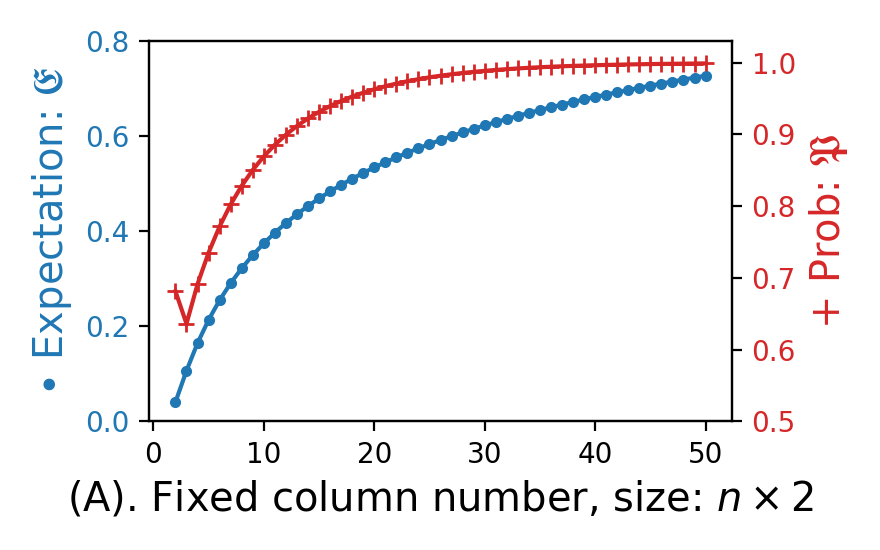
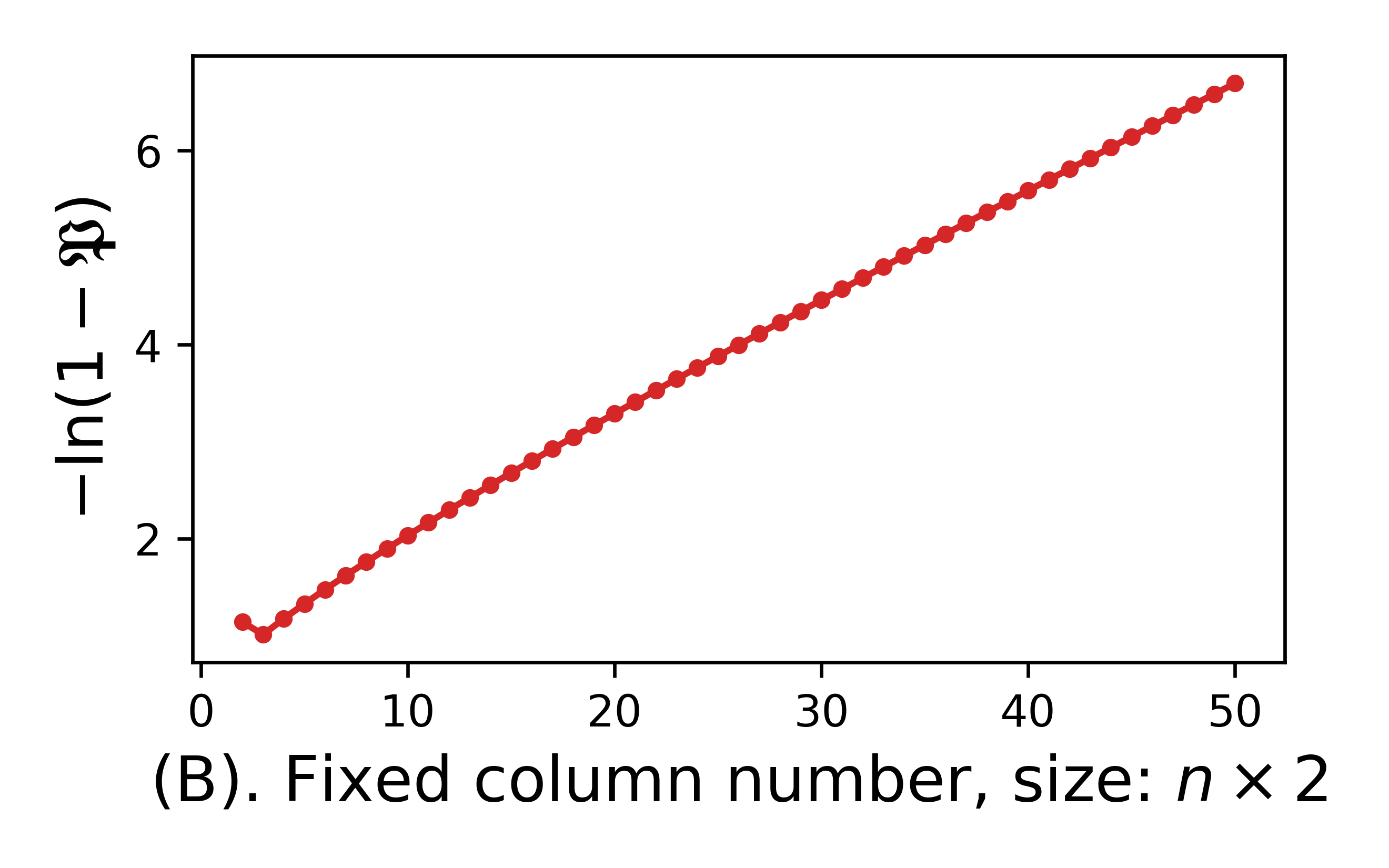
Two-column Cases. Consider the case where 𝐌𝐌\mathbf{M} is of shape n×2𝑛2n\times 2 with the two columns sampled from Δn1superscriptΔ𝑛1\Delta^{n-1} uniformly and independently, we simulated for n=2,3,,50𝑛2350n=2,3,\dots,50 with a size-1010superscript101010^{10} Monte Carlo method for each n𝑛n to calculate 𝔓𝔓\mathfrak{P} and 𝔈𝔈\mathfrak{E}. The result is shown in Fig. 2(A)(B).

We can reduce the calculation of 𝔈𝔈\mathfrak{E} to a numerical integral 𝔈=(Δn1)2ln(i=1n𝐱i𝐲i)d𝐱d𝐲lnnn1n𝔈subscriptsuperscriptsuperscriptΔ𝑛12superscriptsubscript𝑖1𝑛subscript𝐱𝑖subscript𝐲𝑖differential-d𝐱differential-d𝐲𝑛𝑛1𝑛\mathfrak{E}=\int_{(\Delta^{n\!-\!1})^{2}}\ln\left(\sum_{i=1}^{n}\frac{\mathbf{x}_{i}}{\mathbf{y}_{i}}\right)\mathrm{d}\mathbf{x}\mathrm{d}\mathbf{y}-\ln n-\frac{n-1}{n}. 333Details can be found in Supplementary Material.

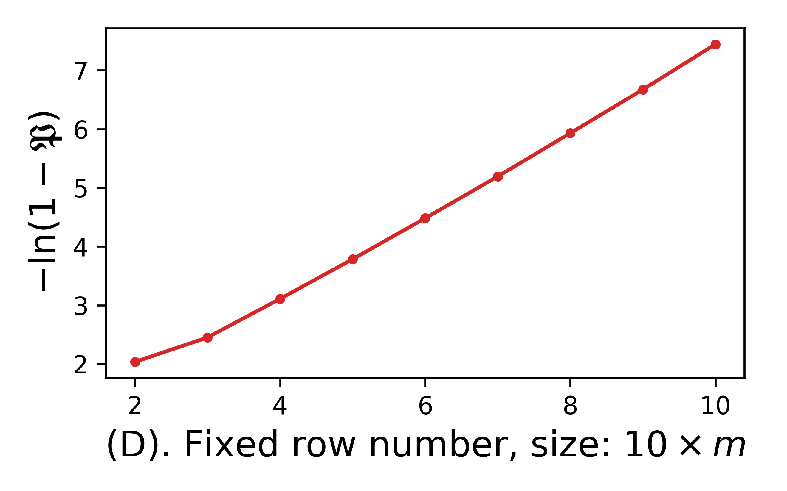
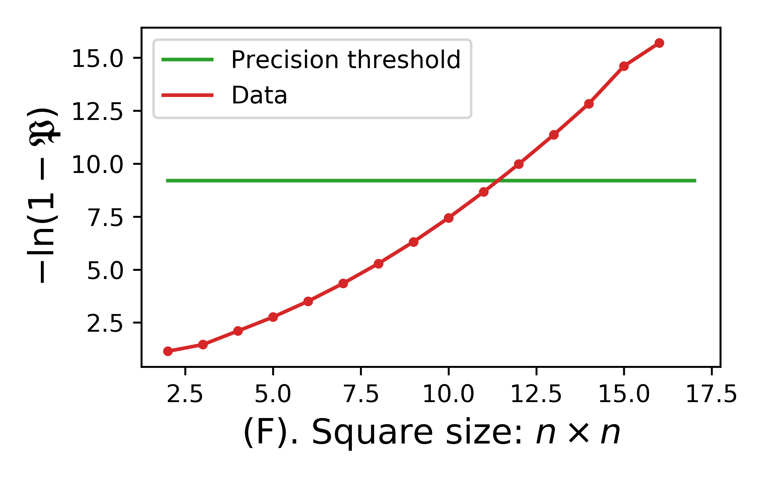
Since 𝔓𝔓\mathfrak{P} goes too close to 111 as the rank grows, we use ln(1𝔓)1𝔓-\ln(1-\mathfrak{P}) to show the increasing in detail. 444We guess an empirical formula ln(1𝔓)12ln(x(x+1)/(x1.5))+0.1x0.31𝔓12𝑥𝑥1𝑥1.50.1𝑥0.3-\ln(1-\mathfrak{P})\approx\frac{1}{2}\ln(x(x+1)/(x-1.5))+0.1x-0.3, see Supplementary Material.

Refer to caption
Refer to caption
Refer to caption

Refer to caption Refer to caption Refer to caption

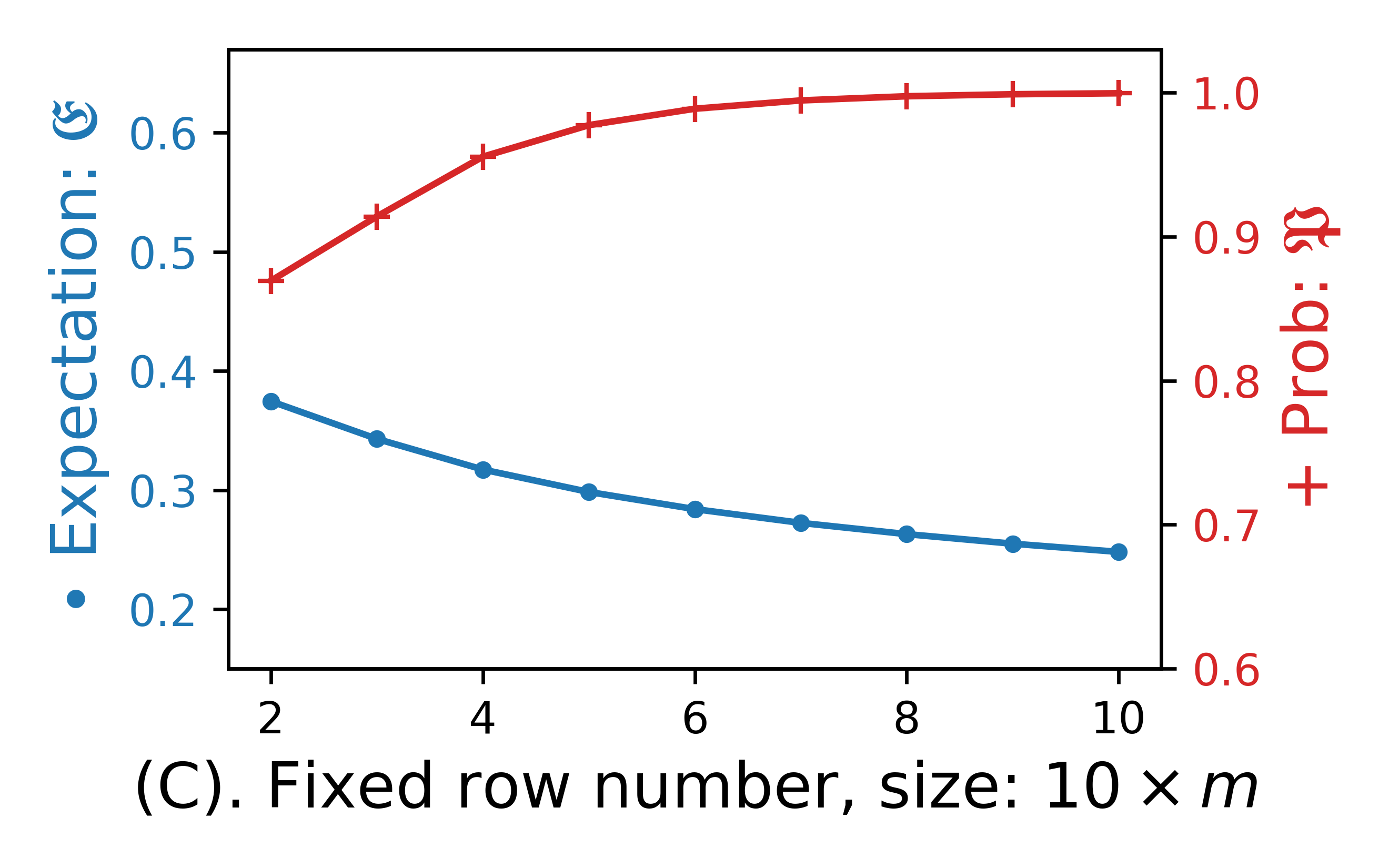
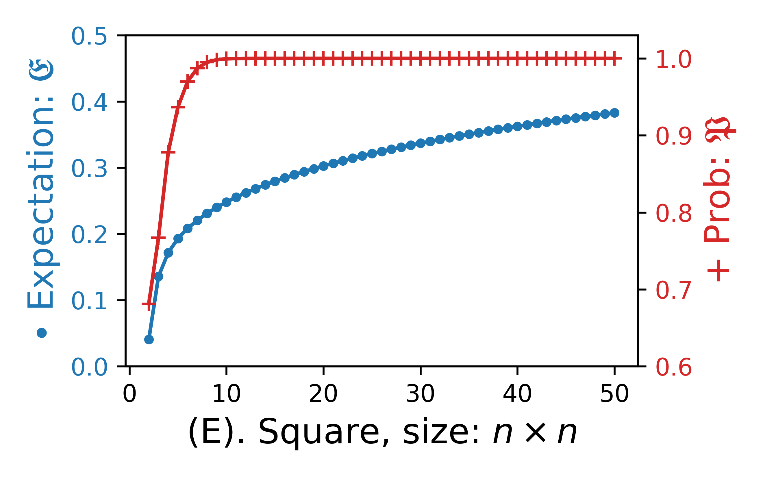
Figure 2: Comparison of RoC between BI and SCBI. (A), (C), (E): the comparison on 𝔓𝔓\mathfrak{P} in blue and on 𝔈𝔈\mathfrak{E} in red. (B), (D), (F): plotting ln(1𝔓)1𝔓-\ln(1-\mathfrak{P}). (A), (B): two-column case, number of rows from 222 to 505050. Monte Carlo of 1010superscript101010^{10} samples for each point on figure. (C), (D): 10-row case, number of columns from 222 to 101010. Monte Carlo of size 108superscript10810^{8}. (E), (F): square case, number of rows from 222 to 505050. Monte Carlo of size 108superscript10810^{8}. The horizontal line in (F) is the theoretical threshold of precision by central limit theorem. For n>17𝑛17n>17, MC provides 𝔓=1𝔓1\mathfrak{P}=1 (s>bsuperscriptssuperscriptb\mathfrak{R}^{\text{s}}>\mathfrak{R}^{\text{b}} for all samples). From the figures, except in (C) where 𝔈𝔈\mathfrak{E} decays slowly when column number grows, the two values 𝔈𝔈\mathfrak{E} and 𝔓𝔓\mathfrak{P} increases as size grows in all the other cases. Moreover, 𝔓𝔓\mathfrak{P} grows to 111 logistically in all situations.

More Columns of a Fixed Row Size. To verify the general cases, we simulated 𝔓𝔓\mathfrak{P} and 𝔈𝔈\mathfrak{E} by Monte Carlo on matrices of 101010-row and various-column shapes, see Fig. 2(C)(D). We sampled 108superscript10810^{8} different 𝐌𝐌\mathbf{M} of shape 10×m10𝑚10\times m for each 2m102𝑚102\leq m\leq 10. Empirical results show that 𝔈𝔈\mathfrak{E} decreases slowly but 𝔓𝔓\mathfrak{P} still increase logistically as m𝑚m grows.

Square Matrices. Fig. 2(E)(F) shows the square cases with size from 222 to 505050, simulated by size 108superscript10810^{8} Monte Carlo.

The empirical 𝔓𝔓\mathfrak{P} is the mean of N𝑁N (sample-size) i.i.d. variables valued 00 or 111, thus the standard deviation of a single variable is smaller than 111. By Central Limit Theorem, the standard deviation σ(𝔓)<N1/2𝜎𝔓superscript𝑁12\sigma(\mathfrak{P})<N^{-1/2} (precision threshold). So we draw lines y=N1/2𝑦superscript𝑁12y=N^{-1/2} in each log-figure, but only in one figure the line lies in the view area.

In all simulated cases, we observe that 𝔈>0𝔈0\mathfrak{E}>0 and 𝔓>0.5𝔓0.5\mathfrak{P}>0.5, indicating that SCBI converges faster than BI in most cases and in average. It is also observed that SCBI behaves even better as matrix size grows, especially when the teacher has more choices on the data to be chosen (i.e., more rows).

4.2 Distribution of Inference Results

The promises of cooperation is that one may infer hypotheses from small amounts of data. Hence, we compare SCBI with BI after small, fixed numbers of rounds.

We sample matrices of shape 20×20202020\times 20 whose columns are distributed evenly in Δ19superscriptΔ19\Delta^{19} to demonstrate. Equivalently, they are column-normalizations of the uniformly sampled matrices whose sum of all entries is one.

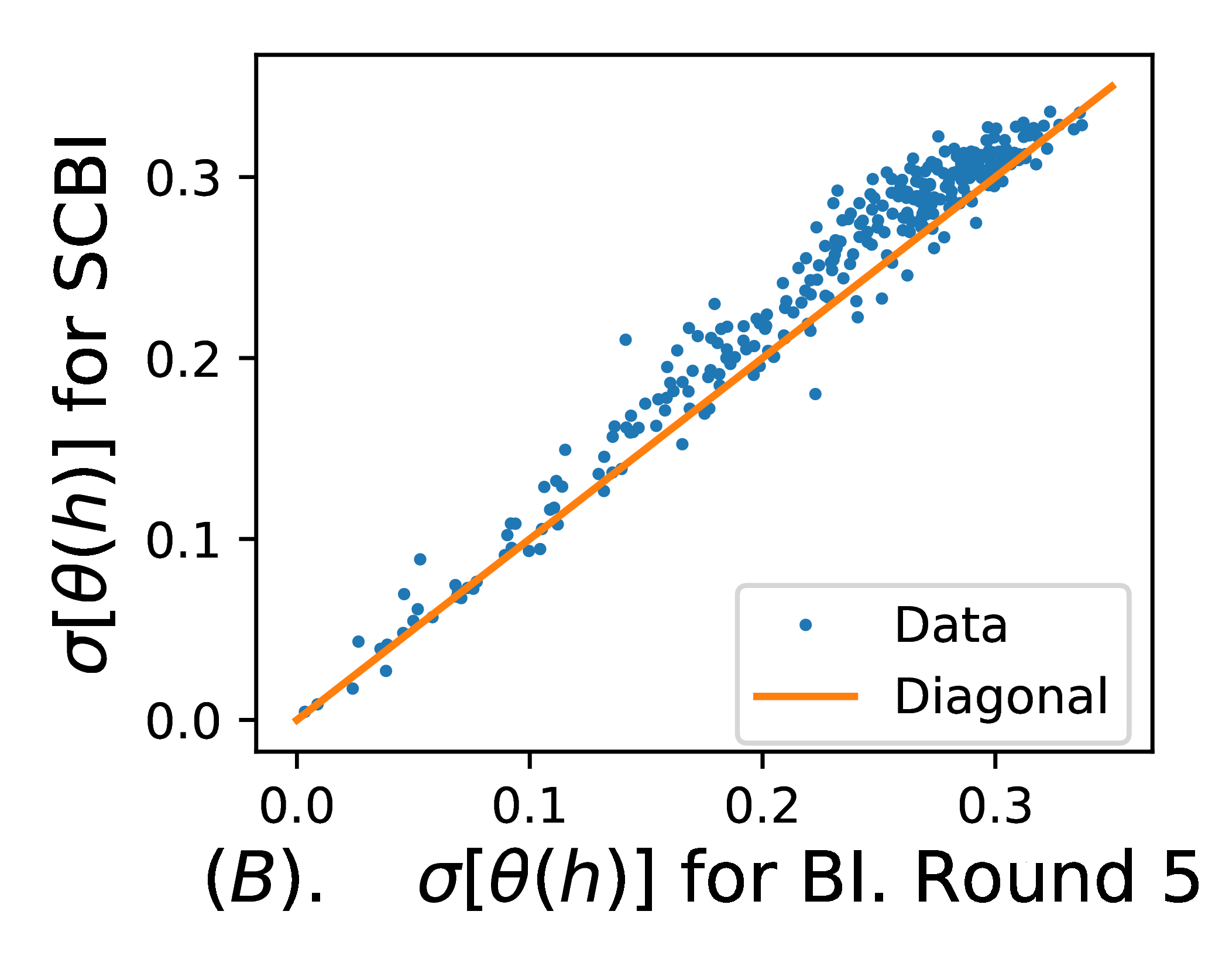
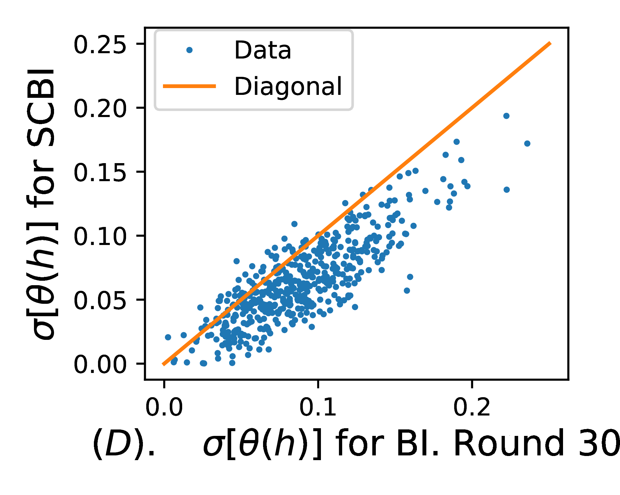
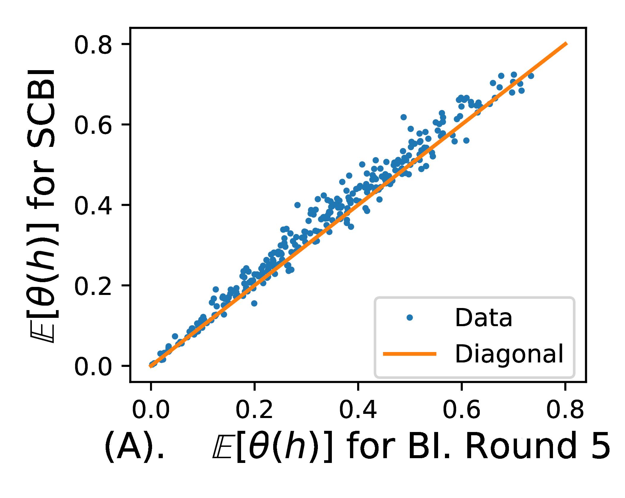
Assume that the correct hypothesis to teach is h𝒫()𝒫h\in\mathcal{P}(\mathcal{H}) We first simulate a 555-round inference behavior, exploring all possible ways that the teacher may teach, then calculate the expectation and standard deviation of θ(h)𝜃\theta(h). With 300300300 matrices sampled in the above way, Fig. 3 shows this comparison between BI and SCBI.
Refer to caption
Refer to caption
Refer to caption
Refer to caption
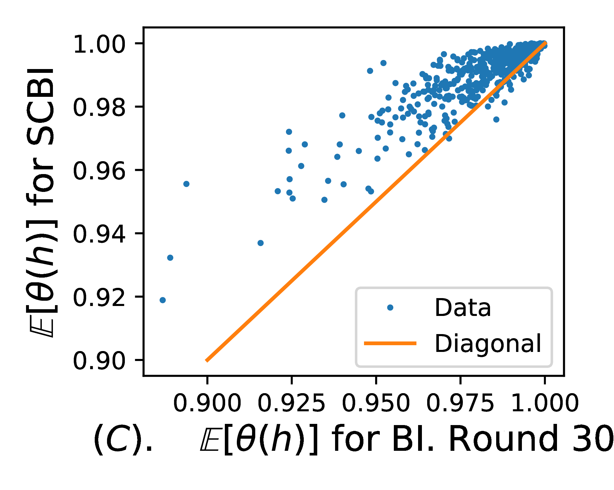
Figure 3: Comparison between BI and SCBI on 20×20202020\times 20 matrices: Top: 300300300 points (matrices) of round 555 accurate value. Bottom: 500500500 points of round 303030 using Monte Carlo of size 200020002000. Left: comparison on expectations of learner’s posterior on hh. Right: comparison on the standard deviations. Orange line is the diagonal.

Similarly, we extend the number of rounds to 303030 by Monte Carlo since an exact calculation on exhausting all possible teaching paths becomes impossible. With sampling 500500500 matrices independently, we simulate a teacher teaches 200020002000 times to round 303030 for each matrix, and the statistics are also shown in Fig. 3. From Fig. 3, we observe that SCBI have better expectation and less variance in the short run.

In conclusion, experiments indicate that SCBI is both more efficient asymptotically, and in the short run.

5 Stability

In this section, we study the robustness of SCBI by setting the initial conditions of teacher and learner different. This could happen when agents do not have full access to their partner’s exact state.

Theory. In this section, we no longer have assumption (iii). Let 𝐓𝐓\mathbf{T} and 𝐋𝐋\mathbf{L} be matrices of teacher and learner (not necessarily have (iii)). Let θ0Tsuperscriptsubscript𝜃0𝑇\theta_{0}^{T} and θ0Lsuperscriptsubscript𝜃0𝐿\theta_{0}^{L} be elements in 𝒫()𝒫\mathcal{P}(\mathcal{H}) representing the prior on hypotheses that the teacher and learner use in the estimation of inference (teacher) and in the actual inference (learner), i.e., μ0T=δθ0Tsuperscriptsubscript𝜇0𝑇subscript𝛿superscriptsubscript𝜃0𝑇\mu_{0}^{T}=\delta_{\theta_{0}^{T}} and μ0L=δθ0Lsuperscriptsubscript𝜇0𝐿subscript𝛿superscriptsubscript𝜃0𝐿\mu_{0}^{L}=\delta_{\theta_{0}^{L}}. During the inference, let μkTsuperscriptsubscript𝜇𝑘𝑇\mu_{k}^{T} and μkLsuperscriptsubscript𝜇𝑘𝐿\mu_{k}^{L} be the distribution of posteriors of the teacher and the learner after round k𝑘k, and denote the corresponding random variables by θkTsuperscriptsubscript𝜃𝑘𝑇\theta_{k}^{T} and θkLsuperscriptsubscript𝜃𝑘𝐿\theta_{k}^{L}, for all positive k𝑘k and \infty, where \infty represents the limit in probability.

Let DD\mathrm{D} be a random variable on 𝒟𝒟\mathcal{D}, we define an operator ΨD𝐋:𝒫(𝒫())𝒫(𝒫()):superscriptsubscriptΨD𝐋𝒫𝒫𝒫𝒫\Psi_{\mathrm{D}}^{\mathbf{L}}:\mathcal{P}(\mathcal{P}(\mathcal{H}))\longrightarrow\mathcal{P}(\mathcal{P}(\mathcal{H})) similar to the ΨΨ\Psi in Section 3. Let Td(θ)=𝐋(d,_)nθsubscript𝑇𝑑𝜃subscriptsuperscript𝐋delimited-⟨⟩𝑛𝜃𝑑_T_{d}(\theta)=\mathbf{L}^{\left\langle n\theta\right\rangle}_{(d,\_)}, then d(ΨD𝐋(μ))(θ):=d𝒟P(D=d)d(Tdμ)(θ)assigndsuperscriptsubscriptΨD𝐋𝜇𝜃subscript𝑑𝒟PD𝑑dsubscript𝑇𝑑𝜇𝜃\mathrm{d}(\Psi_{\mathrm{D}}^{\mathbf{L}}(\mu))(\theta):=\sum\limits_{d\in\mathcal{D}}{\mathrm{P}(\mathrm{D}=d)}\mathrm{d}(T_{d\ast}\mu)(\theta).

Proposition 5.1.

Given a sequence of identical independent 𝒟𝒟\mathcal{D}-valued random variables (Di)i1subscriptsubscriptD𝑖𝑖1(\mathrm{D}_{i})_{i\geq 1} following the uniform distribution. Let μ0𝒫(𝒫())subscript𝜇0𝒫𝒫\mu_{0}\in\mathcal{P}(\mathcal{P}(\mathcal{H})) be a prior distribution on 𝒫()𝒫\mathcal{P}(\mathcal{H}), and μk+1=ΨDk+1𝐋(μk)subscript𝜇𝑘1superscriptsubscriptΨsubscriptD𝑘1𝐋subscript𝜇𝑘\mu_{k+1}=\Psi_{\mathrm{D}_{k+1}}^{\mathbf{L}}(\mu_{k}), then μksubscript𝜇𝑘\mu_{k} converges, in probability, to iaiδisubscript𝑖subscript𝑎𝑖subscript𝛿𝑖\sum_{i\in\mathcal{H}}a_{i}\delta_{i} where ai=𝔼μ0[θ(i)]subscript𝑎𝑖subscript𝔼subscript𝜇0delimited-[]𝜃𝑖a_{i}=\mathbb{E}_{\mu_{0}}\left[\theta(i)\right].

Remark 5.

This proposition helps accelerate the simulation, that one may terminate the teaching process when θkTsuperscriptsubscript𝜃𝑘𝑇\theta_{k}^{T} is sufficiently close to δhsubscript𝛿\delta_{h}, since Prop. 5.1 guarantees that the expectation of the learner’s posterior on the true hypothesis hh at that time is close enough to the eventual probability of getting δhsubscript𝛿\delta_{h}, i.e. 𝔼θL(h)𝔼θkL(h)𝔼superscriptsubscript𝜃𝐿𝔼superscriptsubscript𝜃𝑘𝐿\mathbb{E}\theta_{\infty}^{L}(h)\approx\mathbb{E}\theta_{k}^{L}(h).

Definition 5.2.

We call 𝔼θL(h):=limk𝔼μk(θ(h))assign𝔼superscriptsubscript𝜃𝐿subscript𝑘subscript𝔼subscript𝜇𝑘𝜃\mathbb{E}\theta_{\infty}^{L}(h):=\lim\limits_{k\rightarrow\infty}\mathbb{E}_{\mu_{k}}(\theta(h)) the successful rate of the inference given 𝐓𝐓\mathbf{T}, 𝐋𝐋\mathbf{L}, θ0Tsuperscriptsubscript𝜃0𝑇\theta_{0}^{T} and θ0Lsuperscriptsubscript𝜃0𝐿\theta_{0}^{L}. By the setup in Section 2, the failure probability, 1𝔼θL(h)1𝔼superscriptsubscript𝜃𝐿1-\mathbb{E}\theta_{\infty}^{L}(h), is 12𝔼θLδh112subscriptsuperscriptnorm𝔼superscriptsubscript𝜃𝐿subscript𝛿absent1\frac{1}{2}||\mathbb{E}\theta_{\infty}^{L}-{\delta_{h}}||^{\phantom{|}}_{1}, half of the 111-distance on 𝒫()𝒫\mathcal{P}(\mathcal{H}).

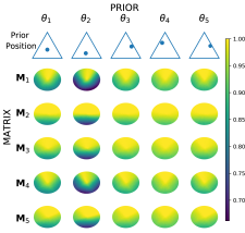
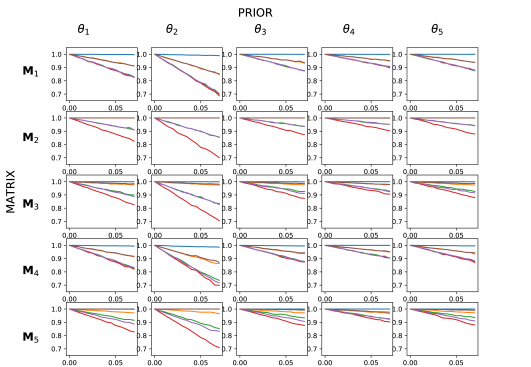
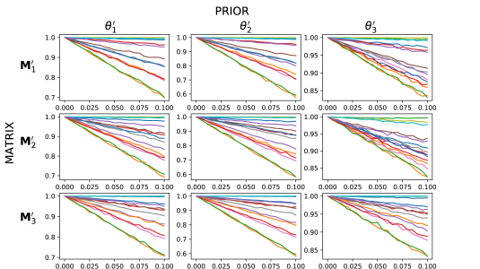
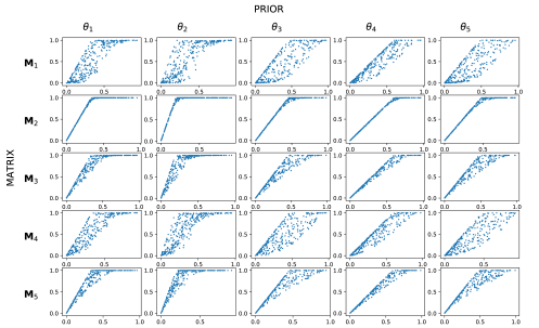
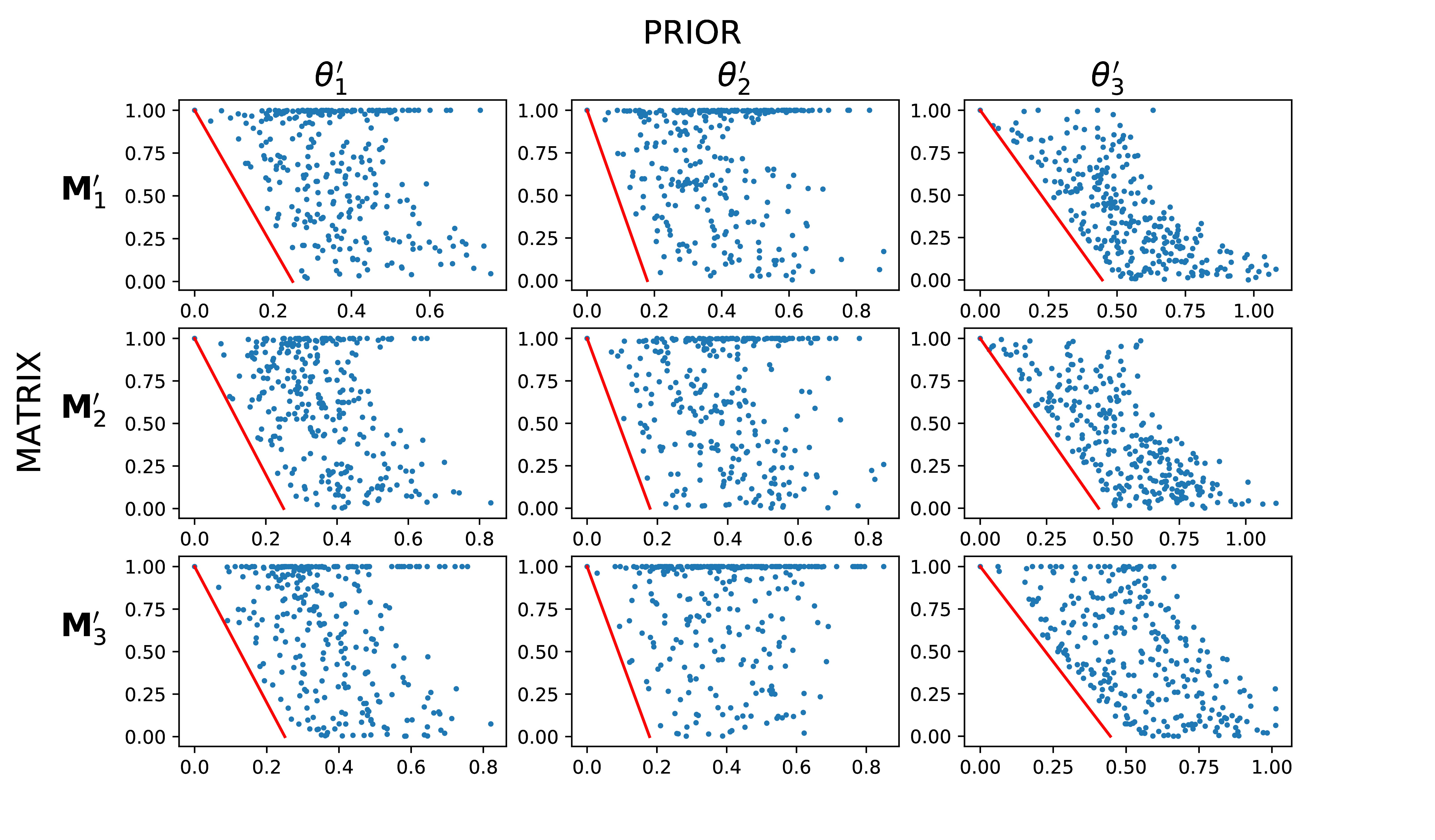
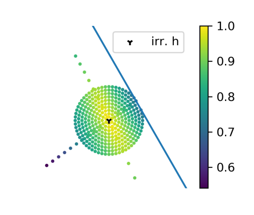
Simulations with Perturbation on Priors. We simulated the square cases of rank 333 and 444. We sample 555 matrices (𝐌1subscript𝐌1\mathbf{M}_{1} to 𝐌5subscript𝐌5\mathbf{M}_{5}) of size 3×3333\times 3, whose columns distribute uniformly on 𝒫({d1,d2,d3})=Δ2𝒫subscript𝑑1subscript𝑑2subscript𝑑3superscriptΔ2\mathcal{P}(\{d_{1},d_{2},d_{3}\})=\Delta^{2}, and 555 priors (θ1subscript𝜃1\theta_{1} to θ5subscript𝜃5\theta_{5}) in 𝒫()𝒫\mathcal{P}(\mathcal{H}), used as θ0Tsuperscriptsubscript𝜃0𝑇\theta_{0}^{T}. Similarly, we sample 333 matrices (𝐌1superscriptsubscript𝐌1\mathbf{M}_{1}^{\prime}, 𝐌2superscriptsubscript𝐌2\mathbf{M}_{2}^{\prime} and 𝐌3superscriptsubscript𝐌3\mathbf{M}_{3}^{\prime}) of size 4×4444\times 4, and 333 priors (θ1superscriptsubscript𝜃1\theta_{1}^{\prime}, θ2superscriptsubscript𝜃2\theta_{2}^{\prime}, θ3superscriptsubscript𝜃3\theta_{3}^{\prime}) from Δ3superscriptΔ3\Delta^{3} in the same way as above. In both cases, we assume h=11h=1\in\mathcal{H} to be the true hypothesis to teach.

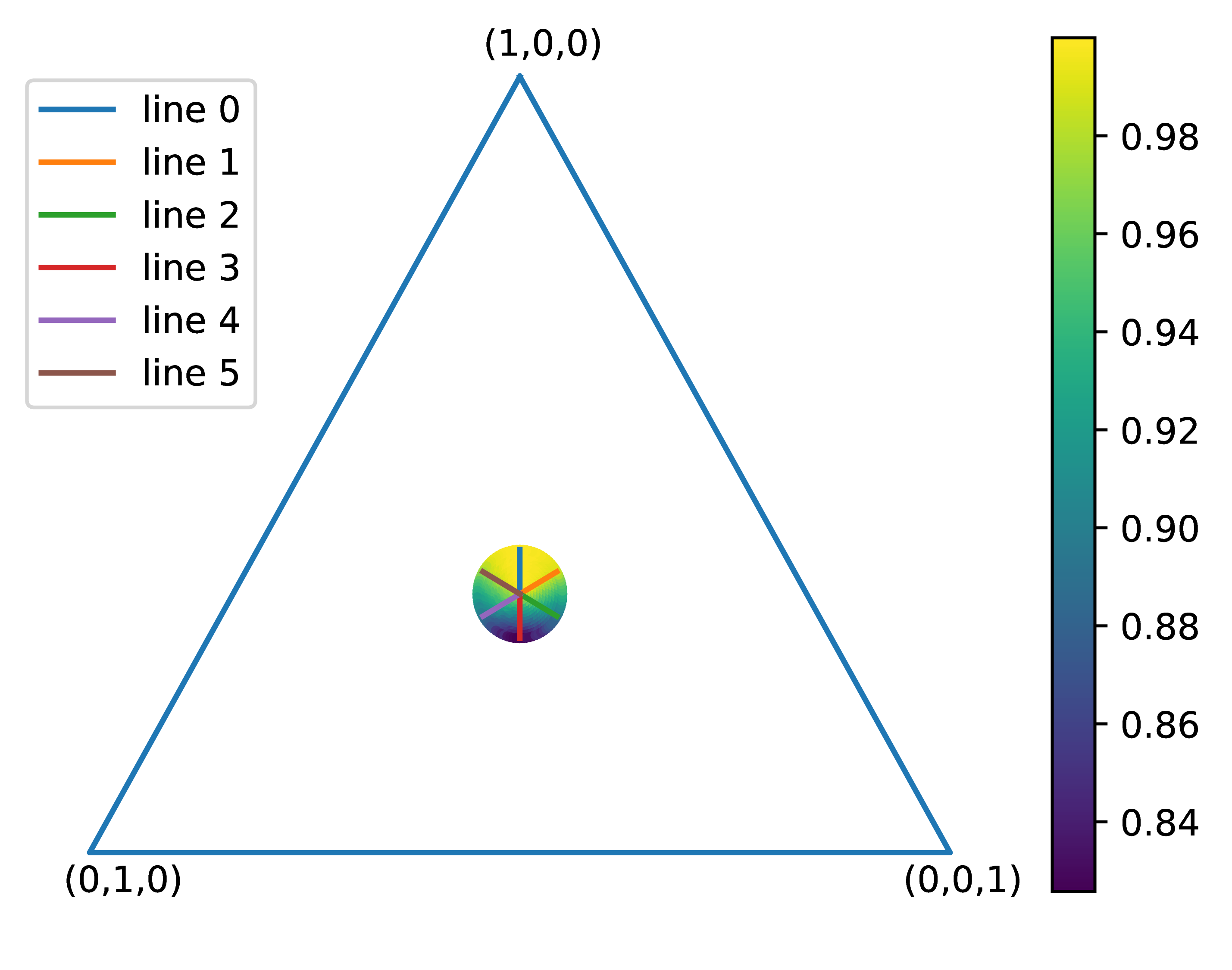
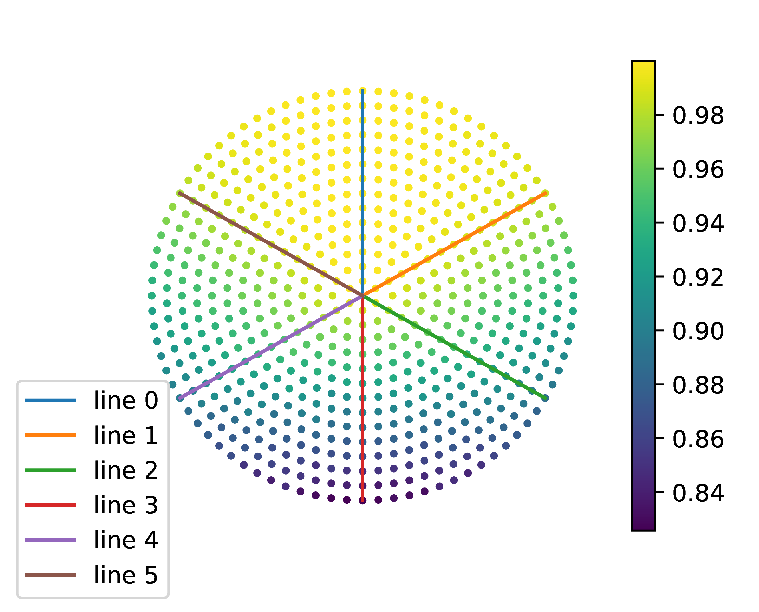
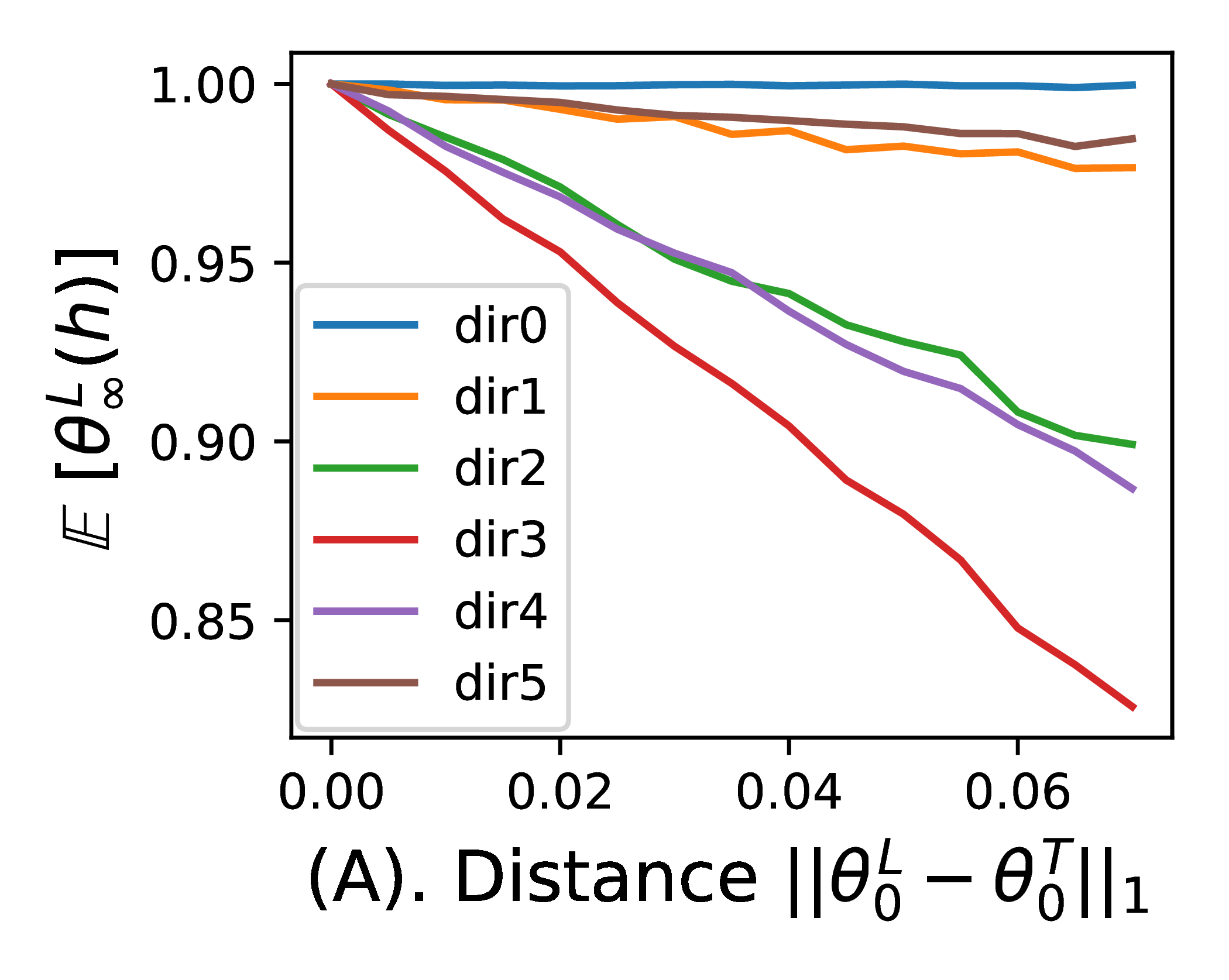
Our simulation is based on Monte Carlo method of 104superscript10410^{4} teaching sequences (for each single point plotted) then use Proposition 5.1 to calculate the successful rate of inference. For 3×3333\times 3 matrices, we perturb θ0Lsuperscriptsubscript𝜃0𝐿\theta_{0}^{L} in two ways: (1) take θ0Lsuperscriptsubscript𝜃0𝐿\theta_{0}^{L} around θ0Tsuperscriptsubscript𝜃0𝑇\theta_{0}^{T} distributed evenly on concentric circles, thus 630630630 points for each θ0Tsuperscriptsubscript𝜃0𝑇\theta_{0}^{T} are taken. In this area, there are 848484 points lying on 666 given directions (60superscript6060^{\circ} apart, see Supplementary Material for figures). (2) sample θ0Lsuperscriptsubscript𝜃0𝐿\theta_{0}^{L} evenly in the whole simplex 𝒫()=Δ2𝒫superscriptΔ2\mathcal{P}(\mathcal{H})=\Delta^{2} (300300300 points for each θ0Tsuperscriptsubscript𝜃0𝑇\theta_{0}^{T}). For 4×4444\times 4 matrices, we perturb θ0Lsuperscriptsubscript𝜃0𝐿\theta_{0}^{L} in two ways: (1) along 151515 randomly chosen directions in Δ3superscriptΔ3\Delta^{3} evenly take 212121 points on each direction, and (2) sample 300300300 points evenly in Δ3superscriptΔ3\Delta^{3}. Then we have the following figure samples (for figures demonstrating the entire simulation, please see Supplementary Material).
Refer to caption
Refer to caption
Refer to caption
Refer to caption
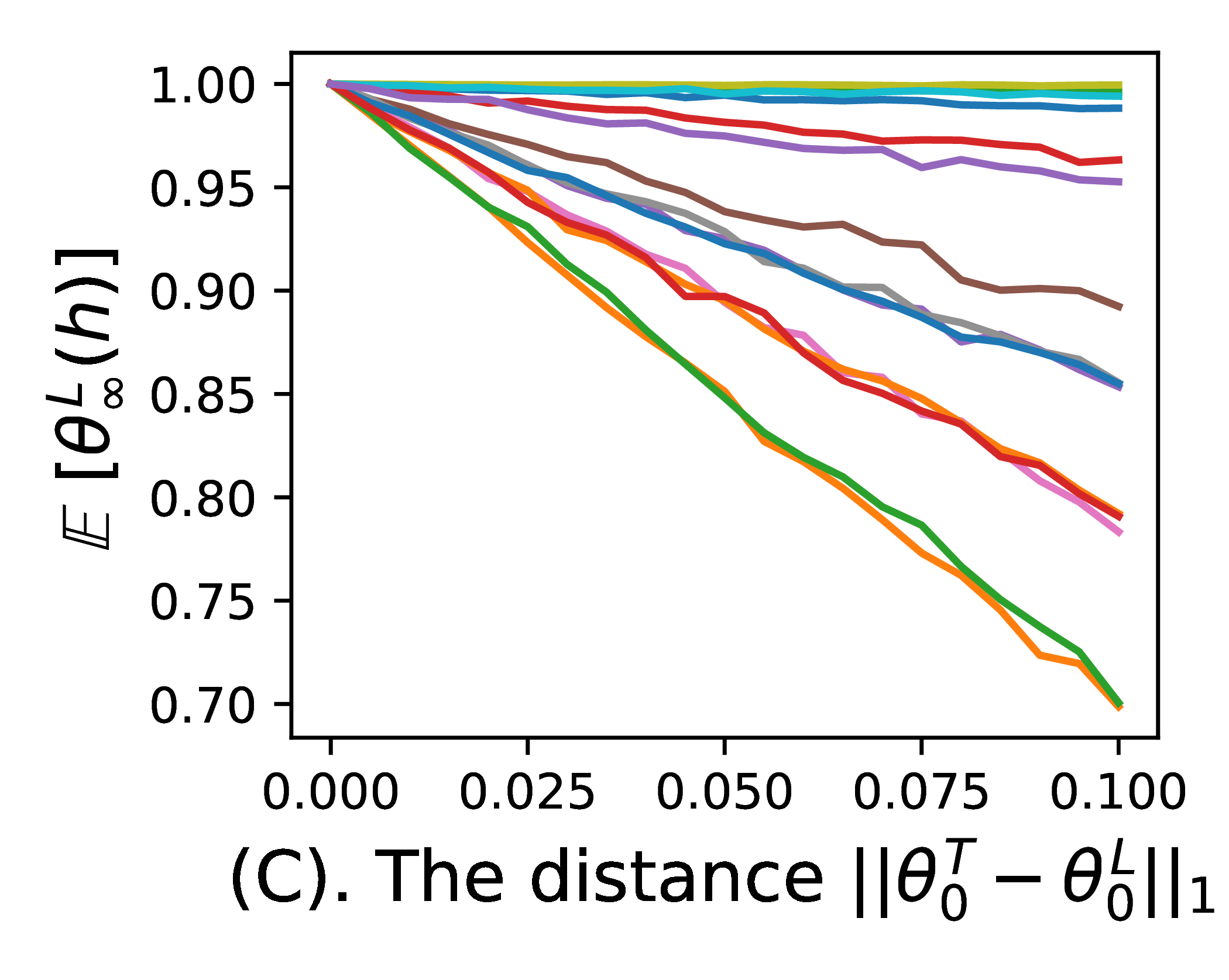
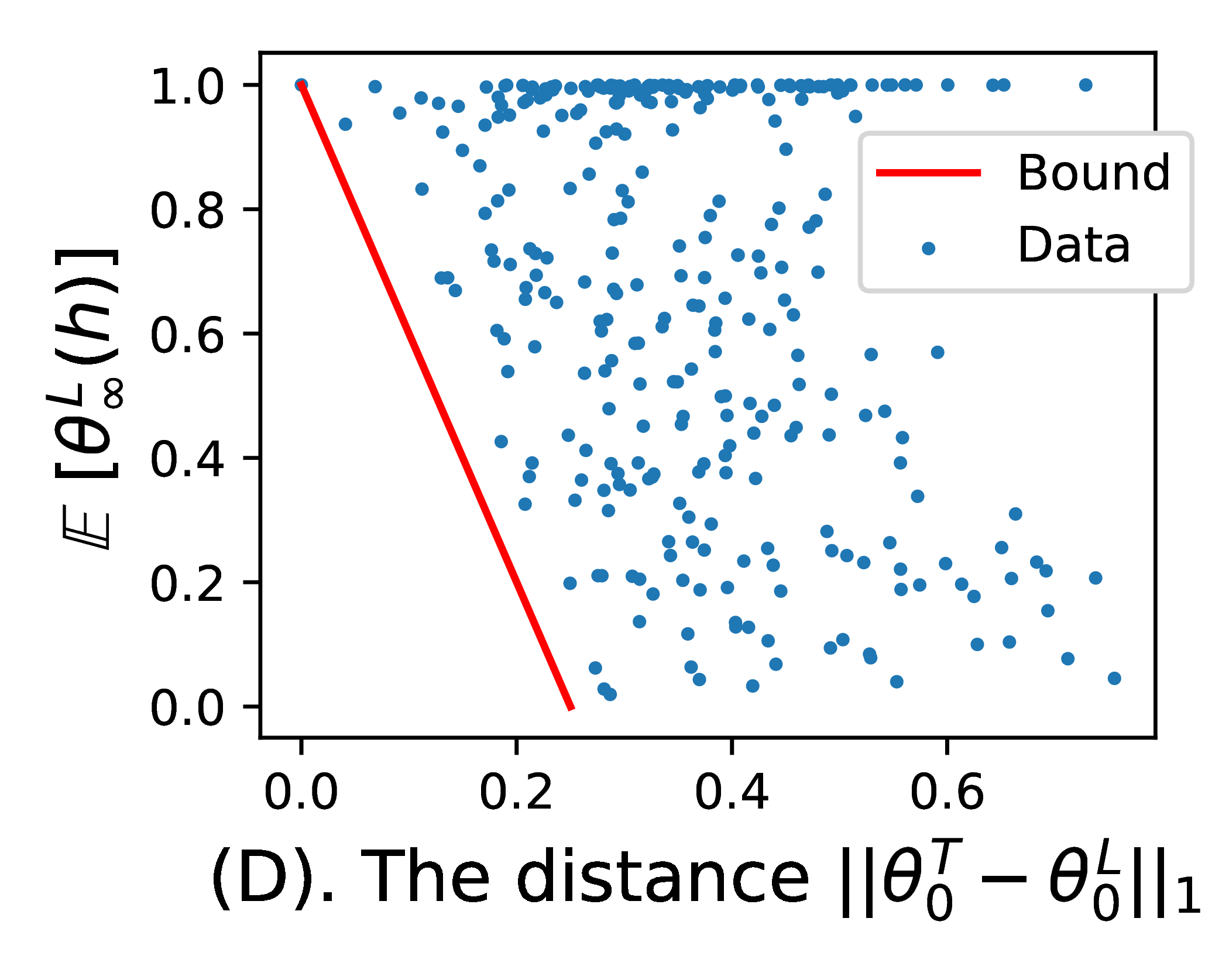
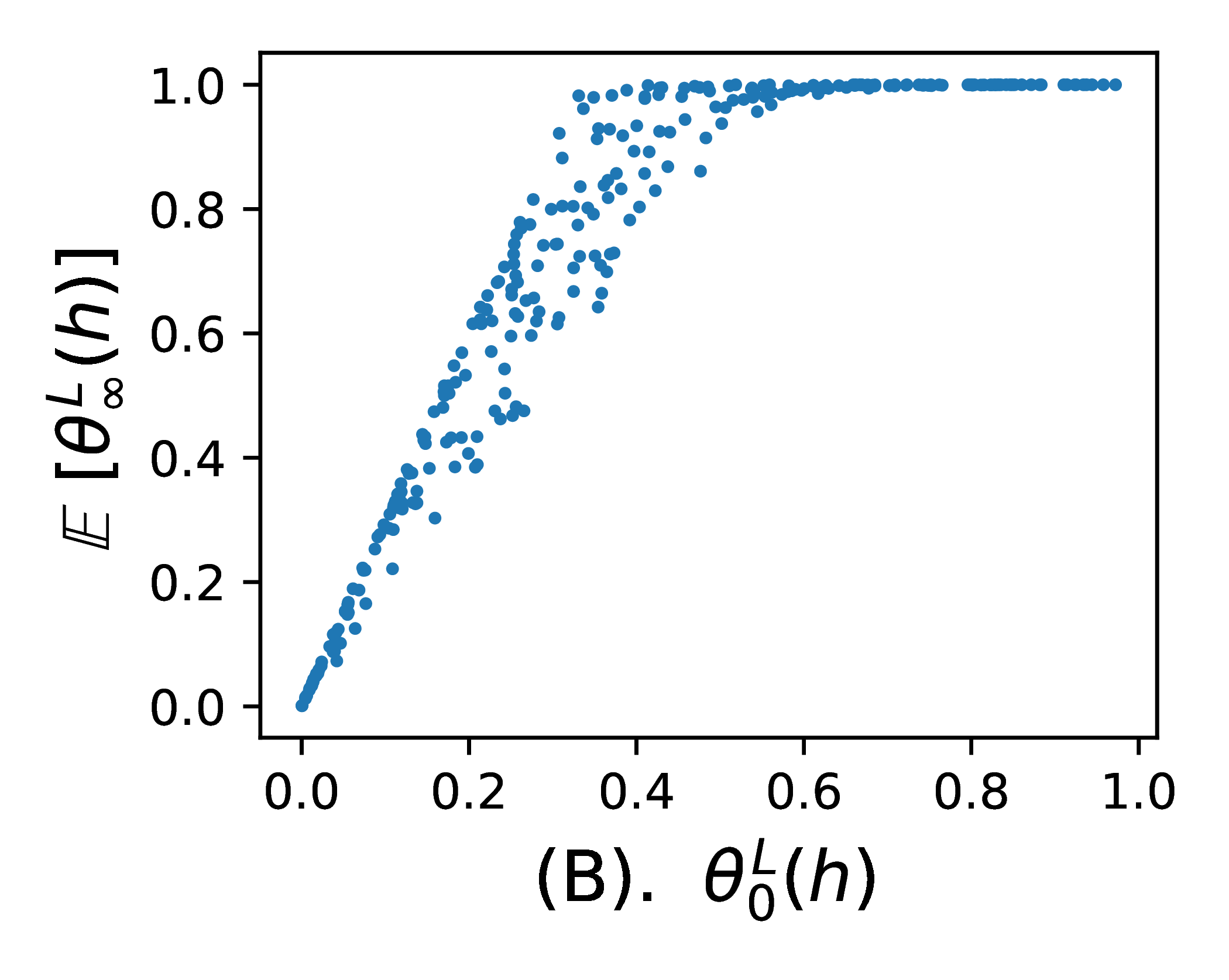
Figure 4: From left to right: (A). Rank 3, 𝐌3subscript𝐌3\mathbf{M}_{3} and θ1subscript𝜃1\theta_{1}, θ0Lsubscriptsuperscript𝜃𝐿0\theta^{L}_{0} is perturbed along six directions. (B). Rank 3, 𝐌3subscript𝐌3\mathbf{M}_{3} and θ1subscript𝜃1\theta_{1}, sample θ0Lsuperscriptsubscript𝜃0𝐿\theta_{0}^{L} uniformly in Δ2superscriptΔ2\Delta^{2}. (C). Rank 4, 𝐌1superscriptsubscript𝐌1\mathbf{M}_{1}^{\prime} and θ1superscriptsubscript𝜃1\theta_{1}^{\prime}, along 151515 different directions. (D). Rank 4, 𝐌1superscriptsubscript𝐌1\mathbf{M}_{1}^{\prime} and θ1superscriptsubscript𝜃1\theta_{1}^{\prime}, sample θ0Lsuperscriptsubscript𝜃0𝐿\theta_{0}^{L} uniformly in Δ3superscriptΔ3\Delta^{3}.

From the figures we see: 1. left pictures indicate that the learner’s expected posterior on hh is roughly linear to perturbations along a line. 2. right pictures indicate that the learner’s expected posterior on hh is closely bounded by a multiple of the learner’s prior on true hh. Thus we have the following conjecture:

Conjecture 5.3.

Given 𝐋=𝐓=𝐌𝐋𝐓𝐌\mathbf{L}=\mathbf{T}=\mathbf{M} and θ0Tsuperscriptsubscript𝜃0𝑇\theta_{0}^{T}, let hh be the true hypothesis to teach. For any ϵ>0italic-ϵ0\epsilon>0, let θ0Lsuperscriptsubscript𝜃0𝐿\theta_{0}^{L} be learner’s prior with a distance to θ0Tsuperscriptsubscript𝜃0𝑇\theta_{0}^{T} less than ϵitalic-ϵ\epsilon. Then the successful rate for sufficiently many rounds is greater than 1Cϵ1𝐶italic-ϵ1-C\epsilon, where C=1θ0T(h)𝐶1superscriptsubscript𝜃0𝑇C=\frac{1}{\theta_{0}^{T}(h)}.

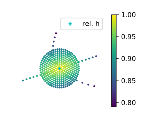
Simulations with Perturbation on Matrices. We now investigate robustness of SCBI to differences between agents’ matrices. Let 𝐓𝐓\mathbf{T} and 𝐋𝐋\mathbf{L} be stochastic, and let 𝐋𝐋\mathbf{L} be perturbed from 𝐓𝐓\mathbf{T}. The simulations are performed on the matrices 𝐌1subscript𝐌1\mathbf{M}_{1} to 𝐌5subscript𝐌5\mathbf{M}_{5} mentioned above with a fixed common prior θ1subscript𝜃1\theta_{1}.

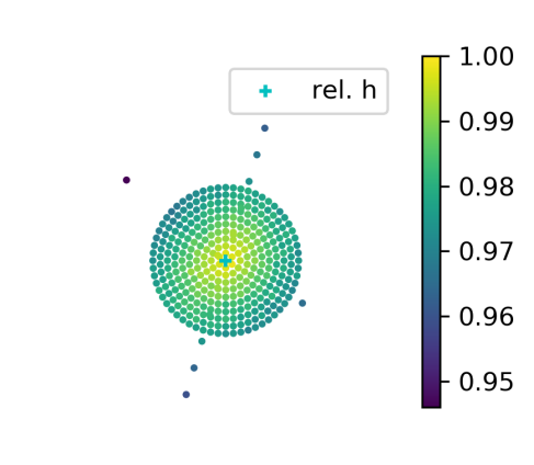
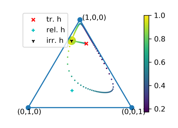
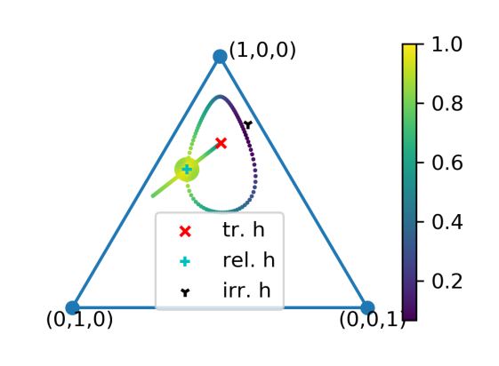
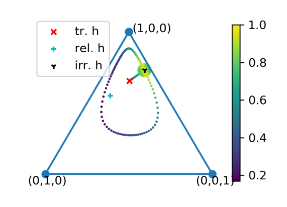
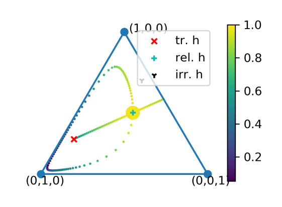
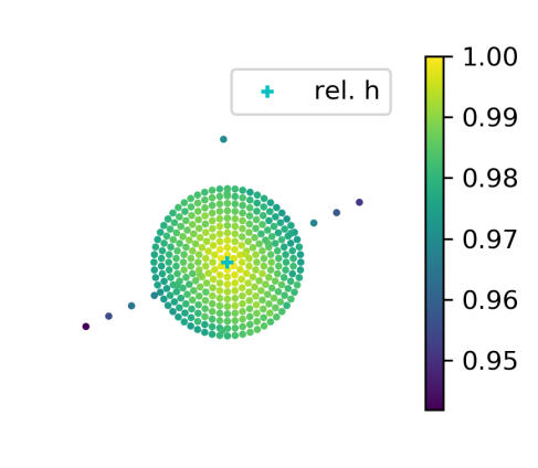
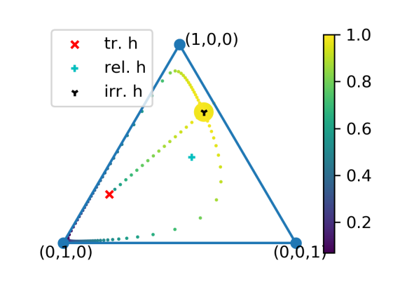
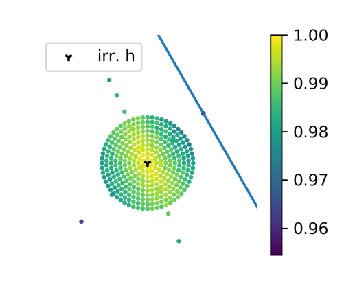
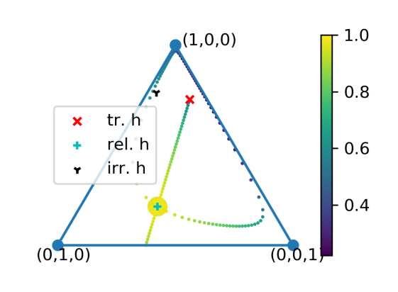
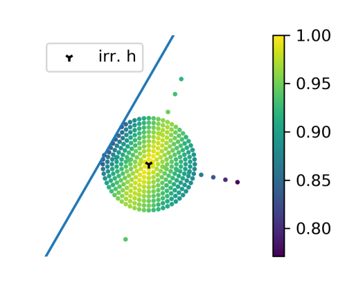
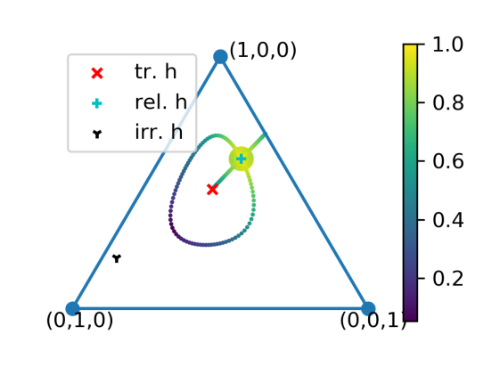
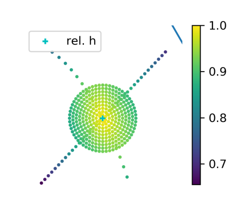
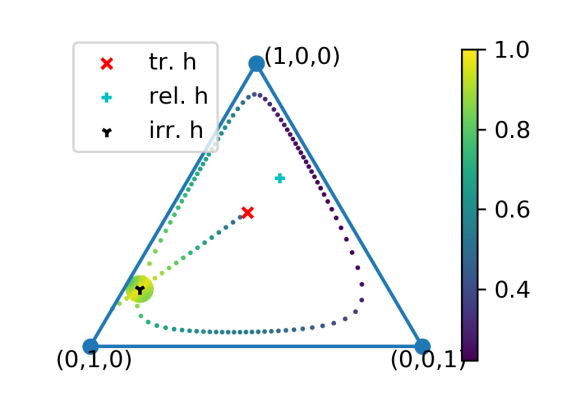
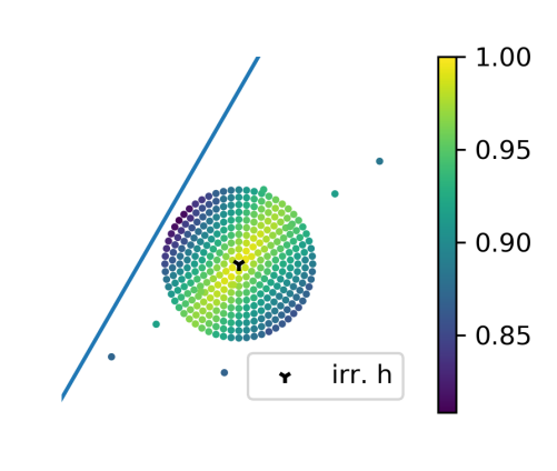
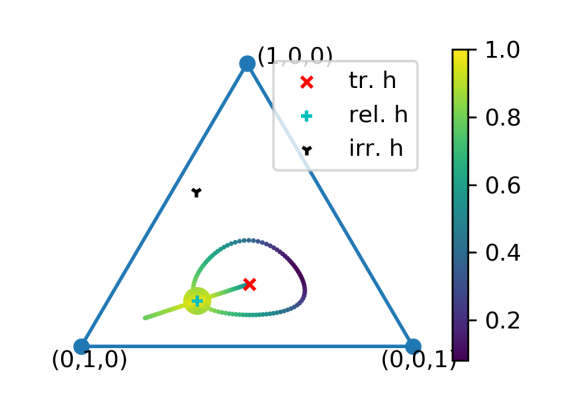
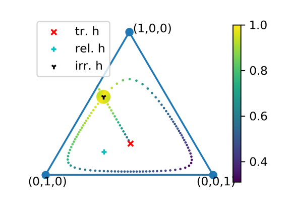
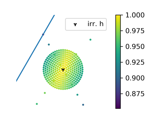
Let all matrices mentioned be column-normalized (this does not affect SCBI since cross-ratios and marginal conditions determines the Sinkhorn scaling results), we call the column determined by the true hypothesis hh (the first column in our simulation) the target column (“tr. h” on Fig. 5), the column which ssuperscripts\mathfrak{R}^{\text{s}} uses (argmin column) the relevant column (“rel. h”) and the other column the irrelevant column (“irr. h”). Let 𝐓𝐓\mathbf{T} be given, and let 𝐋𝐋\mathbf{L} be obtained from 𝐓𝐓\mathbf{T} by perturbing along the relevant / irrelevant column.

Without loss of generality, we assume that only one column of the learner’s matrix 𝐋𝐋\mathbf{L} is perturbed at a time as other perturbations may be treated as compositions of such.

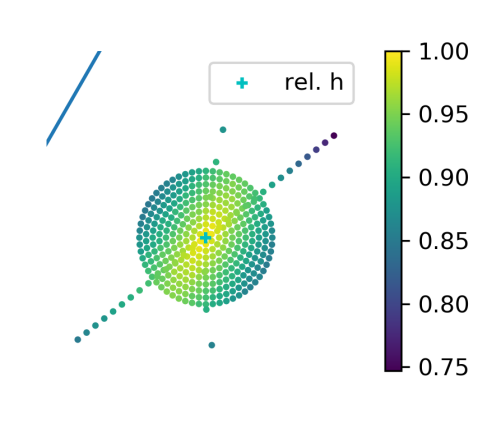
For each 𝐓𝐓\mathbf{T} and each column hsuperscripth^{\prime}, we apply 330330330 perturbations on concentric circles around 𝐓𝐓\mathbf{T} (the disc), 909090 perturbations preserving the normalized-KL divergence (KL(𝐞/n,𝒩vec(𝐋(_,h)/𝐋(_,1),1))KL𝐞𝑛subscript𝒩vecsubscript𝐋_superscriptsubscript𝐋_11\mathrm{KL}(\mathbf{e}/n,\mathscr{N}_{\text{vec}}(\mathbf{L}_{(\_,h^{\prime})}/\mathbf{L}_{(\_,1)},1)) used in ssuperscripts\mathfrak{R}^{\text{s}}) from the target column and 505050 linear interpolations with target column. Each point in Fig. 5 is estimated using a size-104superscript10410^{4} Monte Carlo method using Proposition 5.1.

Refer to caption
Refer to caption
Refer to caption
Refer to caption
Figure 5: The perturbations on 𝐌3subscript𝐌3\mathbf{M}_{3} along a column, and their zoomed-in version (with different color scale). The crosses shows the position of three normalized columns of 𝐓=𝐌3𝐓subscript𝐌3\mathbf{T}=\mathbf{M}_{3}, the location of the dots represent the perturbed column of 𝐓𝐓\mathbf{T} (unperturbed columns are represented by crosses on figures which are not the center of disc) and whereas their colors depict the successful rate of inference. Left two figures are perturbations on the irrelevant column. Right two figures are perturbations on the relevant column.

From the graphs, we can see that the successful rate varies continuously on perturbations, slow on one direction (the yellow strip crossing the center) and rapid on the perpendicular direction (color changed to blue rapidly).

6 Grid World: an Application

Consider a 3×5353\times 5 grid world with two possible terminal goals, A and B, and a starting position S𝑆S as shown below. Let the reward at the terminal position htsubscript𝑡h_{t} be R𝑅R. Assuming no step costs, the value of a grid that distanced k𝑘k from htsubscript𝑡h_{t} is then R×γk𝑅superscript𝛾𝑘R\times\gamma^{k} (in the RL-sense), where γ<1𝛾1\gamma\!<\!1 is the discount factor.

A B
\Uparrow
\Leftarrow S \Rightarrow

Suppose the structure of the world is accessible to both agents whereas the true location of the goal htsubscript𝑡h_{t} is only known to a teacher. The teacher performs a sequence of actions to teach htsubscript𝑡h_{t} to a learner. At each round, there are three available actions, left, up and right. After observing the teacher’s actions, the learner updates their belief on htsubscript𝑡h_{t} accordingly.

We now compare BI and SCBI agents’ behaviours under this grid world. In terms of previous notations, the hypothesis set ={A,B}𝐴𝐵\mathcal{H}=\{A,B\}, the data set 𝒟={left,up,right}𝒟leftupright\mathcal{D}=\{\textit{left},\textit{up},\textit{right}\}. Let the learner’s prior over \mathcal{H} be θ0=(0.5,0.5)subscript𝜃00.50.5\theta_{0}=(0.5,0.5) and the true hypothesis htsubscript𝑡h_{t} be A𝐴A, then at each blue grid, agents’ (unnormalized) initial matrix 𝐌={blockarray}ccc&AB{block}c(cc)leftγ(k1)γ(k+1)upγ(k1)γ(k1)rightγ(k+1)γ(k1)𝐌{blockarray}𝑐𝑐𝑐&𝐴𝐵{block}𝑐𝑐𝑐leftsuperscript𝛾𝑘1superscript𝛾𝑘1upsuperscript𝛾𝑘1superscript𝛾𝑘1rightsuperscript𝛾𝑘1superscript𝛾𝑘1\tiny{\mathbf{M}=\blockarray{ccc}&AB\\ \block{c(cc)}\text{left}\gamma^{(k-1)}\gamma^{(k+1)}\\ \text{up}\gamma^{(k-1)}\gamma^{(k-1)}\\ \text{right}\gamma^{(k+1)}\gamma^{(k-1)}\\ }. Assume both BI teacher and SCBI teacher start with grid S𝑆S. Based on 𝐌𝐌\mathbf{M}, the BI teacher would choose equally between left and up, whereas the SCBI teacher is more likely to choose left as the teacher’s likelihood matrix 𝐓=(2/(3+3γ2)2γ2/(3+3γ2)1/31/32γ2/(3+3γ2)2/(3+3γ2))𝐓matrix233superscript𝛾22superscript𝛾233superscript𝛾213132superscript𝛾233superscript𝛾2233superscript𝛾2\tiny{\mathbf{T}=\begin{pmatrix}2/(3+3\gamma^{2})&2\gamma^{2}/(3+3\gamma^{2})\\ 1/3&1/3\\ 2\gamma^{2}/(3+3\gamma^{2})&2/(3+3\gamma^{2})\end{pmatrix}}, obtained from Sinkhorn scaling on 𝐌𝐌\mathbf{M}, assigns higher probability for left. Hence, comparing to the BI teacher who only aims for the final goal, the SCBI teacher tends to cooperate with the learner by selecting less ambiguous moves towards the goal. This point is aligned with the core idea of many existing models of cooperation in cognitive development (Jara-Ettinger et al., 2016; Bridgers et al., in press), pragmatic reasoning (Frank & Goodman, 2012; Goodman & Stuhlmüller, 2013) and robotics (Ho et al., 2016; Fisac et al., 2017).

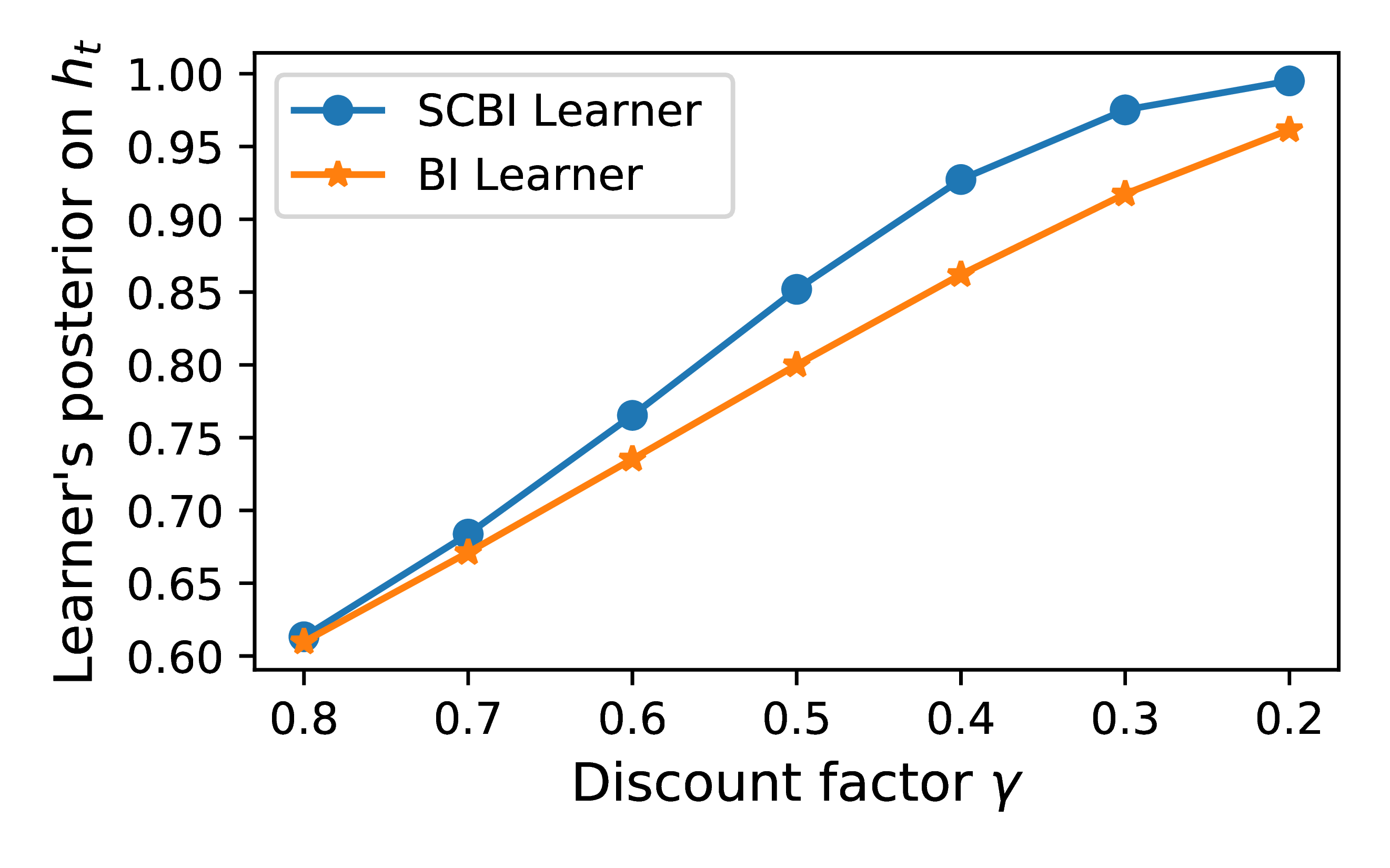
Moreover, even under the same teaching data, the SCBI learner is more likely to infer htsubscript𝑡h_{t} than the BI learner. For instance, given the teacher’s trajectory {left,up}leftup\{\textit{left},\textit{up}\}, the left plot in Fig. 6 shows the SCBI and BI learners’ posteriors on the true hypothesis htsubscript𝑡h_{t}. Hence, comparing to the BI learner who reads the teacher’s action literally, the SCBI learner interprets teacher’s data corporately by updating belief sequentially after each round.
Refer to caption
Refer to caption
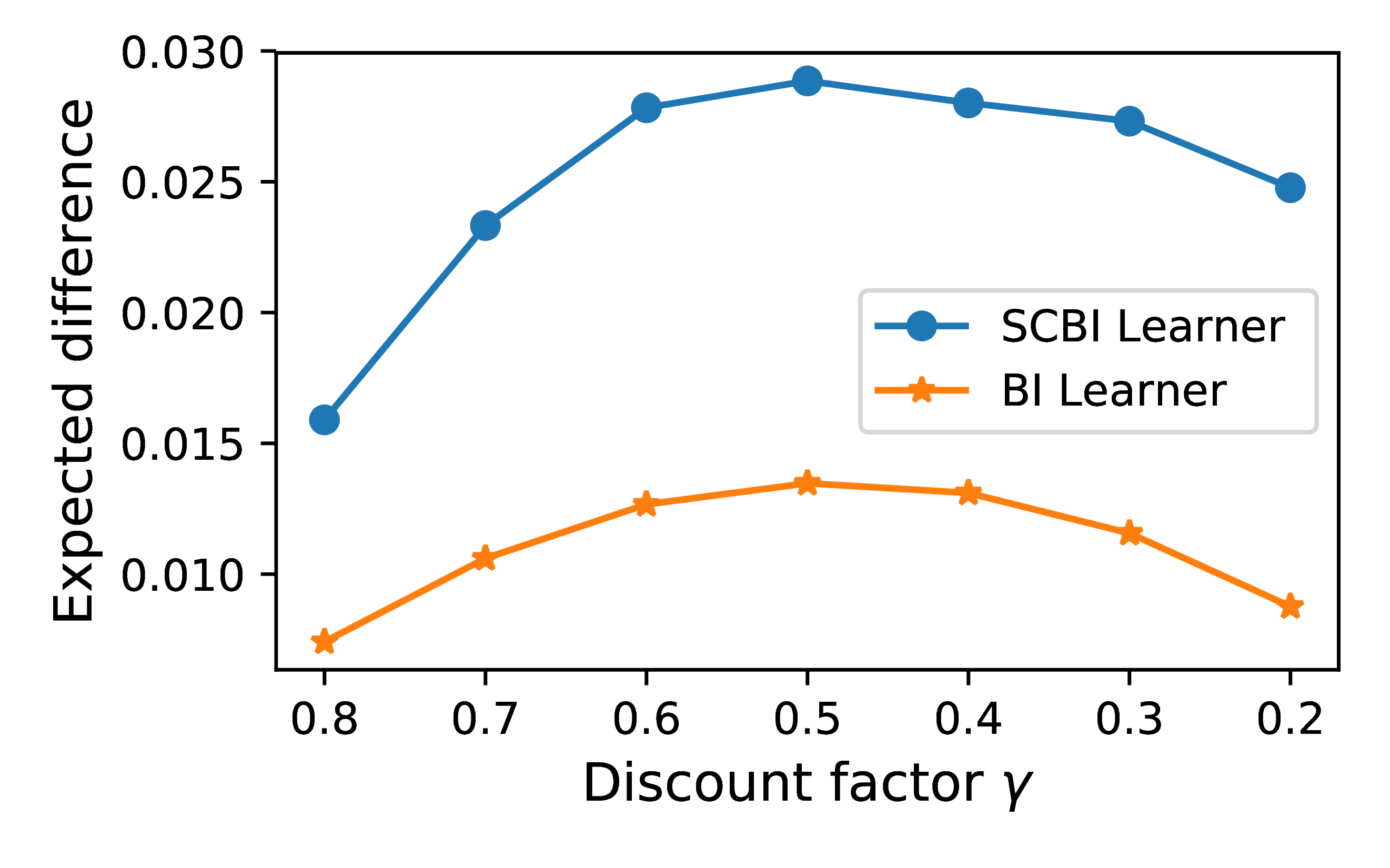
Figure 6: The top plot demonstrates that both BI and SCBI converge to the true hypothesis with SCBI having higher sample efficiency. The bottom plot shows that both BI and SCBI agents are robust to perturbations with SCBI relatively less stable.

Regarding the stability, consider the case where the learner’s discount factor is either greater or less (with equal probability) than the teacher’s by 0.1. The right plot in Fig. 6 illustrates the expected difference between the learner’s posterior on htsubscript𝑡h_{t} after observing a teacher’s trajectory of length 222 and the teacher’s estimation of it.

As discussed in Sec 4.1, showing in Fig. 2, as the board gets wider and the number of possible goals gets more (i.e. the number of hypotheses increases), the gap between posteriors of SCBI and BI learners will increase whereas the expected difference between agents for the same magnitude of perturbation will decrease. Thus, this example illustrates the consistency, sample efficiency, and stability of SCBI versus BI.

7 Related Work

Literatures on Bayesian teaching (Eaves & Shafto, 2016; Eaves Jr et al., 2016), Rational Speech act theory (Frank & Goodman, 2012; Goodman & Stuhlmüller, 2013), and machine teaching (Zhu, 2015, 2013) consider the problem of selecting examples that improve a learner’s chances of inferring a concept. These literatures differ in that they consider the single step, rather than sequential problem, that they do not formalize learners who reason about the teacher’s selection process, and that they models without a mathematical analysis.

The literature on pedagogical reasoning in human learning (Shafto & Goodman, 2008; Shafto et al., 2012, 2014) and cooperative inference (Yang et al., 2018; Wang et al., 2019a, b) in machine learning formalize full recursive reasoning from the perspectives of both the teacher and the learner. These only consider the problem of a single interaction between the teacher and learner.

The literature on curriculum learning considers sequential interactions with a learner by a teacher in which the teacher presents data in an ordered sequence (Bengio et al., 2009), and traces back to various literatures on human and animal learning (Skinner, 1958; Elman, 1993). Curriculum learning involves one of a number of methods for optimizing the sequence of data presented to the learner, most commonly starting with easier / simpler examples first and gradually moving toward more complex or less typical examples. Curriculum learning considers only problems where the teacher optimizes the sequence of examples, where the learner does not reason about the teaching.

8 Conclusions

Cooperation is central to learning in humans and machines. We set out to provide a mathematical foundation for sequential cooperative Bayesian inference (SCBI). We presented new analytic results demonstrating the consistency and asymptotic rate of convergence of SCBI. Empirically, we demonstrated the sample efficiency and stability to perturbations as compared to Bayesian inference, and illustrated with a simple reinforcement learning problem. We therefore provide strong evidence that SCBI satisfies basic desiderata. Future work will aim to provide mathematical proofs of the empirically observed efficiency and stability.

Appendix A Proof of Consistency Theorems

A.1 Proof of Theorem A.1

Theorem A.1.

[Theorem 3.1,(Miescke & Liese, 2008, Theorem 7.115)] In BI, the sequence of posteriors (Sk)subscript𝑆𝑘(S_{k}) is strongly consistent at θ^=δh^𝜃subscript𝛿\widehat{\theta}=\delta_{h} for each hh\in\mathcal{H}, with arbitrary choice of an interior point θ0(𝒫())subscript𝜃0superscript𝒫\theta_{0}\in(\mathcal{P}(\mathcal{H}))^{\circ} (i.e. θ0(h)>0subscript𝜃00\theta_{0}(h)>0 for all hh\in\mathcal{H}) as prior.

Proof.

We follow the same line as discussed right after this theorem in the paper. Let θ0=(θ0(1),θ0(2),,θ0(n))subscript𝜃0subscript𝜃01subscript𝜃02subscript𝜃0𝑛\theta_{0}=(\theta_{0}(1),\theta_{0}(2),\dots,\theta_{0}(n)) be the original prior, and let θk=(θk(1),θk(2),,θk(m))subscript𝜃𝑘subscript𝜃𝑘1subscript𝜃𝑘2subscript𝜃𝑘𝑚\theta_{k}=(\theta_{k}(1),\theta_{k}(2),\dots,\theta_{k}(m)) be the posterior after having k𝑘k data points d1,d2,,dksubscript𝑑1subscript𝑑2subscript𝑑𝑘d_{1},d_{2},\dots,d_{k}. Then for lk𝑙𝑘l\leq k and hh\in\mathcal{H}, the posterior θl(i)=(𝒩vec(diag(𝐌(dl,_))θl1))(i)subscript𝜃𝑙𝑖subscript𝒩vecdiagsubscript𝐌subscript𝑑𝑙_subscript𝜃𝑙1𝑖\theta_{l}(i)=\left(\mathscr{N}_{\text{vec}}(\mathrm{diag}(\mathbf{M}_{(d_{l},\_)})\theta_{l-1})\right)(i) by Bayes’ rule. In other words,

θl(i)=𝐌(dl,i)[θ(l1)(i)]j=1m𝐌(dl,j)[θ(l1)(j)].subscript𝜃𝑙𝑖subscript𝐌subscript𝑑𝑙𝑖delimited-[]subscript𝜃𝑙1𝑖superscriptsubscript𝑗1𝑚subscript𝐌subscript𝑑𝑙𝑗delimited-[]subscript𝜃𝑙1𝑗\theta_{l}(i)=\dfrac{\mathbf{M}_{(d_{l},i)}[\theta_{(l-1)}(i)]}{\sum_{j=1}^{m}\mathbf{M}_{(d_{l},j)}[\theta_{(l-1)}(j)]}. (5)

This is a recursive formula, so we may move forward to calculate θl(i)subscript𝜃𝑙𝑖\theta_{l}(i) from a smaller round index θt(i)subscript𝜃𝑡𝑖\theta_{t}(i) with t<l𝑡𝑙t<l:

θl(i)=[s=tl𝐌(ds,i)]θ(t1)(i)j=1m[s=tl𝐌(ds,j)]θ(t1)(j).subscript𝜃𝑙𝑖delimited-[]superscriptsubscriptproduct𝑠𝑡𝑙subscript𝐌subscript𝑑𝑠𝑖subscript𝜃𝑡1𝑖superscriptsubscript𝑗1𝑚delimited-[]superscriptsubscriptproduct𝑠𝑡𝑙subscript𝐌subscript𝑑𝑠𝑗subscript𝜃𝑡1𝑗\theta_{l}(i)=\dfrac{\left[\prod_{s=t}^{l}\mathbf{M}_{(d_{s},i)}\right]\theta_{(t-1)}(i)}{\sum_{j=1}^{m}\left[\prod_{s=t}^{l}\mathbf{M}_{(d_{s},j)}\right]\theta_{(t-1)}(j)}.

This recursion stops at prior θ0subscript𝜃0\theta_{0}, so we have an explicit expression of θksubscript𝜃𝑘\theta_{k}:

θk(i)=[s=1k𝐌(ds,i)]θ0(i)j=1m[s=1k𝐌(ds,j)]θ0(j).subscript𝜃𝑘𝑖delimited-[]superscriptsubscriptproduct𝑠1𝑘subscript𝐌subscript𝑑𝑠𝑖subscript𝜃0𝑖superscriptsubscript𝑗1𝑚delimited-[]superscriptsubscriptproduct𝑠1𝑘subscript𝐌subscript𝑑𝑠𝑗subscript𝜃0𝑗\theta_{k}(i)=\dfrac{\left[\prod_{s=1}^{k}\mathbf{M}_{(d_{s},i)}\right]\theta_{0}(i)}{\sum_{j=1}^{m}\left[\prod_{s=1}^{k}\mathbf{M}_{(d_{s},j)}\right]\theta_{0}(j)}. (6)

It can be seen that for each hypothesis i𝑖i, the denominator of the k𝑘k-th posterior on i𝑖i are the same, so we have

θk(i)θk(h)=[s=1k𝐌(ds,i)]θ0(i)[s=1k𝐌(ds,h)]θ0(h).subscript𝜃𝑘𝑖subscript𝜃𝑘delimited-[]superscriptsubscriptproduct𝑠1𝑘subscript𝐌subscript𝑑𝑠𝑖subscript𝜃0𝑖delimited-[]superscriptsubscriptproduct𝑠1𝑘subscript𝐌subscript𝑑𝑠subscript𝜃0\dfrac{\theta_{k}(i)}{\theta_{k}(h)}=\dfrac{\left[\prod_{s=1}^{k}\mathbf{M}_{(d_{s},i)}\right]\theta_{0}(i)}{\left[\prod_{s=1}^{k}\mathbf{M}_{(d_{s},h)}\right]\theta_{0}(h)}. (7)

So we define αk(d)subscript𝛼𝑘𝑑\alpha_{k}(d) to be the frequency of the occurrence of data d𝑑d in the first k𝑘k rounds of a episode. And then

log(θk(i)θk(h))=log(θ0(i)θ0(h))+d=1nαk(d)log(𝐌(d,i)𝐌(d,h)).subscript𝜃𝑘𝑖subscript𝜃𝑘subscript𝜃0𝑖subscript𝜃0superscriptsubscript𝑑1𝑛subscript𝛼𝑘𝑑subscript𝐌𝑑𝑖subscript𝐌𝑑\small\log\left(\dfrac{\theta_{k}(i)}{\theta_{k}(h)}\right)=\log\left(\dfrac{\theta_{0}(i)}{\theta_{0}(h)}\right)+\sum_{d=1}^{n}\alpha_{k}(d)\log\left(\dfrac{\mathbf{M}_{(d,i)}}{\mathbf{M}_{(d,h)}}\right). (8)

Since we know that the data (di)subscript𝑑𝑖(d_{i}) in the model is sampled following the i.i.d. with distribution 𝐌(_,h)subscript𝐌_\mathbf{M}_{(\_,h)}, then for a fixed k𝑘k, αk(i)subscript𝛼𝑘𝑖\alpha_{k}(i) follows the multinomial distribution with parameter 𝐌(_,h)subscript𝐌_\mathbf{M}_{(\_,h)}.

By the strong law of large numbers, αk(i)k𝐌(i,h)subscript𝛼𝑘𝑖𝑘subscript𝐌𝑖\frac{\alpha_{k}(i)}{k}\rightarrow\mathbf{M}_{(i,h)} almost surely as k𝑘k\rightarrow\infty. Thus, when we rewrite the sample values to random variable version,

1klog(Θk(i)Θk(h))d=1n𝐌(d,h)log(𝐌(d,i)𝐌(d,h))a.s.1𝑘subscriptΘ𝑘𝑖subscriptΘ𝑘superscriptsubscript𝑑1𝑛subscript𝐌𝑑subscript𝐌𝑑𝑖subscript𝐌𝑑a.s.\dfrac{1}{k}\log\left(\dfrac{\Theta_{k}(i)}{\Theta_{k}(h)}\right)\rightarrow\sum_{d=1}^{n}\mathbf{M}_{(d,h)}\log\left(\dfrac{\mathbf{M}_{(d,i)}}{\mathbf{M}_{(d,h)}}\right)\quad\text{a.s.} (9)

That is,

1klog(Θk(i)Θk(h))KL(𝐌(_,h),𝐌(_,i))a.s.1𝑘subscriptΘ𝑘𝑖subscriptΘ𝑘KLsubscript𝐌_subscript𝐌_𝑖a.s.\dfrac{1}{k}\log\left(\dfrac{\Theta_{k}(i)}{\Theta_{k}(h)}\right)\longrightarrow-\mathrm{KL}\left(\mathbf{M}_{(\_,h)},\mathbf{M}_{(\_,i)}\right)\quad\text{a.s.} (10)

By the assumption in Section 2 of the paper that 𝐌𝐌\mathbf{M} has distinct columns, the KL divergence between the i𝑖i-th column and the hh-th column is strictly positive, thus almost surely, log(Θk(i)Θk(h))subscriptΘ𝑘𝑖subscriptΘ𝑘\log\left(\dfrac{\Theta_{k}(i)}{\Theta_{k}(h)}\right)\rightarrow-\infty, or equivalently, Θk(i)Θk(h)0subscriptΘ𝑘𝑖subscriptΘ𝑘0\dfrac{\Theta_{k}(i)}{\Theta_{k}(h)}\rightarrow 0, for any ih𝑖i\neq h.

Therefore, θk=(θk(1),θk(2),,θk(m))δhsubscript𝜃𝑘subscript𝜃𝑘1subscript𝜃𝑘2subscript𝜃𝑘𝑚subscript𝛿\theta_{k}=(\theta_{k}(1),\theta_{k}(2),\dots,\theta_{k}(m))\rightarrow\delta_{h} almost surely, equivalently, BI at θ^^𝜃\widehat{\theta} is strongly consistent. ∎

A.2 Proof of Theorem 3.2

Theorem A.2 (Theorem 3.2).

In BI, with θ^=δh^𝜃subscript𝛿\widehat{\theta}=\delta_{h} for some hh\in\mathcal{H}, let Θk(h)(D1,,Dk):=Sk(h|D1,,Dk)assignsubscriptΘ𝑘subscriptD1subscriptD𝑘subscript𝑆𝑘conditionalsubscriptD1subscriptD𝑘\Theta_{k}(h)(\mathrm{D}_{1},\dots,\mathrm{D}_{k}):=S_{k}(h|\mathrm{D}_{1},\dots,\mathrm{D}_{k}) be the hh-component of posterior given D1,,DksubscriptD1subscriptD𝑘\mathrm{D}_{1},\dots,\mathrm{D}_{k} as random variables valued in 𝒟𝒟\mathcal{D}. Then 1klog(Θk(h)1Θk(h))1𝑘subscriptΘ𝑘1subscriptΘ𝑘\dfrac{1}{k}\log\left(\dfrac{\Theta_{k}(h)}{1-\Theta_{k}(h)}\right) converges to a constant minhh{KL(𝐌(_,h),𝐌(_,h))}subscriptminsuperscriptKLsubscript𝐌_subscript𝐌_superscript\mathrm{min}_{h^{\prime}\neq h}\left\{\mathrm{KL}(\mathbf{{M}}_{(\_,h)},\mathbf{{M}}_{(\_,h^{\prime})})\right\} almost surely.

Proof.

Follow the previous proof. First recall that 1klog(Θk(i)Θk(h))KL(𝐌(_,h),𝐌(_,i))1𝑘subscriptΘ𝑘𝑖subscriptΘ𝑘KLsubscript𝐌_subscript𝐌_𝑖\dfrac{1}{k}\log\left(\dfrac{\Theta_{k}(i)}{\Theta_{k}(h)}\right)\rightarrow-\mathrm{KL}(\mathbf{{M}}_{(\_,h)},\mathbf{{M}}_{(\_,i)}) almost surely. Let η:=argminih{KL(𝐌(_,h),𝐌(_,i))}assign𝜂subscriptargmin𝑖KLsubscript𝐌_subscript𝐌_𝑖\eta:=\mathrm{argmin}_{i\neq h}\left\{\mathrm{KL}(\mathbf{{M}}_{(\_,h)},\mathbf{{M}}_{(\_,i)})\right\}, then Θk(η)subscriptΘ𝑘𝜂\Theta_{k}(\eta) decays slowest among {Θk(i):ih}conditional-setsubscriptΘ𝑘𝑖𝑖\left\{\Theta_{k}(i):i\neq h\right\} almost surely.

Therefore, for the sample values θksubscript𝜃𝑘\theta_{k}’s, asymptotically,

1klog[θk(η)θk(h)]1klog[1θk(h)θk(h)]1klog[(m1)θk(η)θk(h)].1𝑘subscript𝜃𝑘𝜂subscript𝜃𝑘1𝑘1subscript𝜃𝑘subscript𝜃𝑘1𝑘𝑚1subscript𝜃𝑘𝜂subscript𝜃𝑘\small\dfrac{1}{k}\log\left[\dfrac{\theta_{k}(\eta)}{\theta_{k}(h)}\right]\!\leq\!\dfrac{1}{k}\log\left[\dfrac{1-\theta_{k}(h)}{\theta_{k}(h)}\right]\!\leq\!\dfrac{1}{k}\log\left[\dfrac{(m-1)\theta_{k}(\eta)}{\theta_{k}(h)}\right].

So when we are taking limits k𝑘k\rightarrow\infty, with probability one, we have

KL(𝐌(_,h),𝐌(_,η))limk1klog[1θk(h)θk(h)]KLsubscript𝐌_subscript𝐌_𝜂subscript𝑘1𝑘1subscript𝜃𝑘subscript𝜃𝑘\displaystyle-\mathrm{KL}(\mathbf{{M}}_{(\_,h)},\mathbf{{M}}_{(\_,\eta)})\leq\lim_{k\rightarrow\infty}\dfrac{1}{k}\log\left[\dfrac{1-\theta_{k}(h)}{\theta_{k}(h)}\right]
limkKL(𝐌(_,h),𝐌(_,η))+1klog(m1)absentsubscript𝑘KLsubscript𝐌_subscript𝐌_𝜂1𝑘𝑚1\displaystyle\leq\lim_{k\rightarrow\infty}-\mathrm{KL}(\mathbf{{M}}_{(\_,h)},\mathbf{{M}}_{(\_,\eta)})+\dfrac{1}{k}\log(m-1)
=KL(𝐌(_,h),𝐌(_,η)).absentKLsubscript𝐌_subscript𝐌_𝜂\displaystyle=-\mathrm{KL}(\mathbf{{M}}_{(\_,h)},\mathbf{{M}}_{(\_,\eta)}). (11)

A.3 Proof of Theorem 3.5

To prove Theorem A.3, we need the following lemmas.

Lemma A.3.1.

Given a fixed hypothesis hh\in\mathcal{H}, for any μ𝒫(Δm1)𝜇𝒫superscriptΔ𝑚1\mu\in\mathcal{P}(\Delta^{m-1}),

𝔼μ(θ(h))𝔼Ψ(h)(μ)(θ(h)).subscript𝔼𝜇𝜃subscript𝔼Ψ𝜇𝜃\mathbb{E}_{\mu}(\theta(h))\leq\mathbb{E}_{\Psi(h)(\mu)}(\theta(h)). (12)

equality happens when 𝐌(i,h)n𝐱=𝐌(j,h)n𝐱subscriptsuperscript𝐌delimited-⟨⟩𝑛𝐱𝑖subscriptsuperscript𝐌delimited-⟨⟩𝑛𝐱𝑗\mathbf{M}^{\left\langle n\mathbf{x}\right\rangle}_{\phantom{~{}~{}}(i,h)}=\mathbf{M}^{\left\langle n\mathbf{x}\right\rangle}_{\phantom{~{}~{}}(j,h)} for any i𝑖i, j𝑗j and μ𝜇\mu-almost everywhere for 𝐱Δm1𝐱superscriptΔ𝑚1\mathbf{x}\in\Delta^{m-1}.

Remark 6.

This lemma shows that the expectation of θ(h)𝜃\theta(h), in each round is increasing, thus the sequence obtained from all the rounds has an limit since the sequence is monotonic and upper bounded by 111. To prove the theorem we, then just need to show the limit is 111.

Proof.

We start from the right hand side of Eq. 12. Let ΔΔ\Delta denote Δm1superscriptΔ𝑚1\Delta^{m-1} for short.

𝔼Ψ(h)(μ)(θ(h))subscript𝔼Ψ𝜇𝜃\displaystyle\mathbb{E}_{\Psi(h)(\mu)}(\theta(h))
=\displaystyle= Δθ(h)d(Ψ(h)(μ))(θ)subscriptΔ𝜃dΨ𝜇𝜃\displaystyle\!\!\!\!\int_{\Delta}\theta(h)\mathrm{d}(\Psi(h)(\mu))(\theta)
=\displaystyle= Δd=1nτd(Td1(θ))θ(h)d(Td(μ))(θ)subscriptΔsuperscriptsubscript𝑑1𝑛subscript𝜏𝑑superscriptsubscript𝑇𝑑1𝜃𝜃dsubscript𝑇𝑑𝜇𝜃\displaystyle\!\!\!\!\int\limits_{\Delta}\sum_{d=1}^{n}\tau_{d}(T_{d}^{-1}(\theta))\theta(h)\mathrm{d}(T_{d\ast}(\mu))(\theta)
=\displaystyle= d=1nΔτd(θ)(Td(θ))(h)d(Td(μ))(Td(θ))superscriptsubscript𝑑1𝑛subscriptΔsubscript𝜏𝑑𝜃subscript𝑇𝑑𝜃dsubscript𝑇𝑑𝜇subscript𝑇𝑑𝜃\displaystyle\!\!\!\!\sum_{d=1}^{n}\int\limits_{\Delta}\tau_{d}(\theta)(T_{d}(\theta))(h)\mathrm{d}\left(T_{d\ast}(\mu)\right)(T_{d}(\theta))
=\displaystyle= d=1nΔτd(θ)(Td(θ))(h)dμ(θ)superscriptsubscript𝑑1𝑛subscriptΔsubscript𝜏𝑑𝜃subscript𝑇𝑑𝜃differential-d𝜇𝜃\displaystyle\!\!\!\!\sum_{d=1}^{n}\int\limits_{\Delta}\tau_{d}(\theta)(T_{d}(\theta))(h)\mathrm{d}\mu(\theta)
=\displaystyle= d=1nΔTd(θ)(h)nθ(h)Td(θ)(h)dμ(θ)superscriptsubscript𝑑1𝑛subscriptΔsubscript𝑇𝑑𝜃𝑛𝜃subscript𝑇𝑑𝜃differential-d𝜇𝜃\displaystyle\!\!\!\!\sum_{d=1}^{n}\int\limits_{\Delta}\dfrac{T_{d}(\theta)(h)}{n\theta(h)}T_{d}(\theta)(h)\mathrm{d}\mu(\theta)
=\displaystyle= Δd=1nTd(θ)(h)2nθ(h)dμ(θ)subscriptΔsuperscriptsubscript𝑑1𝑛subscript𝑇𝑑𝜃superscript2𝑛𝜃d𝜇𝜃\displaystyle\!\!\!\!\int\limits_{\Delta}\sum_{d=1}^{n}\dfrac{T_{d}(\theta)(h)^{2}}{n\theta(h)}\mathrm{d}\mu(\theta)

In the calculation, the bijectivity of Tdsubscript𝑇𝑑T_{d} and the formula (Td(μ))(E)=μ(Td1(E))subscript𝑇𝑑𝜇𝐸𝜇superscriptsubscript𝑇𝑑1𝐸(T_{d\ast}(\mu))(E)=\mu(T_{d}^{-1}(E)) is used (and will be used repetitively later).

Consider that by definition of the bijection Tdsubscript𝑇𝑑T_{d}, the sum d=1nTd(θ)(h)=nθ(h)superscriptsubscript𝑑1𝑛subscript𝑇𝑑𝜃𝑛𝜃\sum_{d=1}^{n}T_{d}(\theta)(h)=n\theta(h) (Tdsubscript𝑇𝑑T_{d} is the d𝑑d-th row of Sinkhorn scaling by column sums nθ𝑛𝜃n\theta). Thus

𝔼Ψ(h)(μ)(θ(h))subscript𝔼Ψ𝜇𝜃\displaystyle\mathbb{E}_{\Psi(h)(\mu)}(\theta(h)) =\displaystyle= Δd=1nTd(θ)(h)2d=1nTd(θ)(h)dμ(θ)subscriptΔsuperscriptsubscript𝑑1𝑛subscript𝑇𝑑𝜃superscript2superscriptsubscript𝑑1𝑛subscript𝑇𝑑𝜃differential-d𝜇𝜃\displaystyle\!\!\!\!\int\limits_{\Delta}\dfrac{\sum_{d=1}^{n}T_{d}(\theta)(h)^{2}}{\sum_{d=1}^{n}T_{d}(\theta)(h)}\mathrm{d}\mu(\theta) (13)
\displaystyle\geq Δ(d=1nTd(θ)(h))2nd=1nTd(θ)(h)dμ(θ)subscriptΔsuperscriptsuperscriptsubscript𝑑1𝑛subscript𝑇𝑑𝜃2𝑛superscriptsubscript𝑑1𝑛subscript𝑇𝑑𝜃differential-d𝜇𝜃\displaystyle\!\!\!\!\int\limits_{\Delta}\dfrac{\left(\sum_{d=1}^{n}T_{d}(\theta)(h)\right)^{2}}{n\sum_{d=1}^{n}T_{d}(\theta)(h)}\mathrm{d}\mu(\theta)
=\displaystyle= Δ1nd=1nTd(θ)(h)dμ(θ)subscriptΔ1𝑛superscriptsubscript𝑑1𝑛subscript𝑇𝑑𝜃d𝜇𝜃\displaystyle\!\!\!\!\int\limits_{\Delta}\dfrac{1}{n}\sum_{d=1}^{n}T_{d}(\theta)(h)\mathrm{d}\mu(\theta)
=\displaystyle= Δθ(h)dμ(θ)subscriptΔ𝜃differential-d𝜇𝜃\displaystyle\!\!\!\!\int\limits_{\Delta}\theta(h)\mathrm{d}\mu(\theta)
=\displaystyle= 𝔼μ(θ(h)),subscript𝔼𝜇𝜃\displaystyle\mathbb{E}_{\mu}(\theta(h)),

where d=1nTd(θ)(h)21n(d=1nTd(θ)(h))2superscriptsubscript𝑑1𝑛subscript𝑇𝑑𝜃superscript21𝑛superscriptsuperscriptsubscript𝑑1𝑛subscript𝑇𝑑𝜃2\sum_{d=1}^{n}T_{d}(\theta)(h)^{2}\geq\dfrac{1}{n}\left(\sum_{d=1}^{n}T_{d}(\theta)(h)\right)^{2} by Cauchy-Schwarz inequality, with equality achieved if and only if Td(θ)(h)subscript𝑇𝑑𝜃T_{d}(\theta)(h) is constant on d𝑑d. Therefore, the equality of Eq. (13) is achieved when 𝐌(d,h)n𝐱subscriptsuperscript𝐌delimited-⟨⟩𝑛𝐱𝑑\mathbf{M}^{\left\langle n\mathbf{x}\right\rangle}_{\phantom{~{}~{}}(d,h)} is constant on d𝑑d, μ𝜇\mu-almost everywhere for 𝐱Δm1𝐱superscriptΔ𝑚1\mathbf{x}\in\Delta^{m-1}.

θ(h)=0𝜃0\theta(h)=0θ(h)=1𝜃1\theta(h)=1θ(h)=a𝜃𝑎\theta(h)=aθ(h)=b𝜃𝑏\theta(h)=bLemma A.3.4Lemma A.3.2ϵitalic-ϵ\epsilon
Figure 7: Sketch of Δm1superscriptΔ𝑚1\Delta^{m-1}, for a general θ𝜃\theta, its y𝑦y-coordinate is θ(h)𝜃\theta(h). The levels are compatible with proof of Theorem A.3. Lemma A.3.2 and Lemma A.3.4 are located where they contribute to prove the vanishing of measure in the limit.

The following lemmas helps showing that the measure μksubscript𝜇𝑘\mu_{k} of the complement of a neighborhood of δh𝒫()subscript𝛿𝒫\delta_{h}\in\mathcal{P}(\mathcal{H}) has limit 00.

Lemma A.3.2.

Given 𝐌𝐌\mathbf{M}, hh\in\mathcal{H} and prior μ0𝒫(Δm1)subscript𝜇0𝒫superscriptΔ𝑚1\mu_{0}\in\mathcal{P}(\Delta^{m-1}) satisfying assumptions, we have

𝔼μk(θ(h)θ(h))=𝔼μ0(θ(h)θ(h))subscript𝔼subscript𝜇𝑘𝜃superscript𝜃subscript𝔼subscript𝜇0𝜃superscript𝜃\mathbb{E}_{\mu_{k}}\left(\dfrac{\theta(h^{\prime})}{\theta(h)}\right)=\mathbb{E}_{\mu_{0}}\left(\dfrac{\theta(h^{\prime})}{\theta(h)}\right) (14)

for any k0𝑘0k\geq 0 and any hhsuperscripth^{\prime}\neq h.

Proof.

It suffices to prove the k=1𝑘1k=1 case for a general μ0subscript𝜇0\mu_{0} (then we have the rest by induction).

𝔼μ1(θ(h)θ(h))=Δ(θ(h)θ(h))dμ1(θ)subscript𝔼subscript𝜇1𝜃superscript𝜃subscriptΔ𝜃superscript𝜃differential-dsubscript𝜇1𝜃\displaystyle\mathbb{E}_{\mu_{1}}\left(\dfrac{\theta(h^{\prime})}{\theta(h)}\right)=\int\limits_{\Delta}\left(\dfrac{\theta(h^{\prime})}{\theta(h)}\right)\mathrm{d}\mu_{1}(\theta) (15)
=\displaystyle= Δ(θ(h)θ(h))d(Ψ(h)(μ0))(θ)subscriptΔ𝜃superscript𝜃dΨsubscript𝜇0𝜃\displaystyle\int\limits_{\Delta}\left(\dfrac{\theta(h^{\prime})}{\theta(h)}\right)\mathrm{d}(\Psi(h)(\mu_{0}))(\theta)
=\displaystyle= Δd𝒟τd(Td1(θ))θ(h)θ(h)d(Td(μ0))(θ)subscriptΔsubscript𝑑𝒟subscript𝜏𝑑superscriptsubscript𝑇𝑑1𝜃𝜃superscript𝜃dsubscript𝑇𝑑subscript𝜇0𝜃\displaystyle\int\limits_{\Delta}\sum_{d\in\mathcal{D}}\tau_{d}(T_{d}^{-1}(\theta))\dfrac{\theta(h^{\prime})}{\theta(h)}\mathrm{d}(T_{d\ast}(\mu_{0}))(\theta)
=\displaystyle= d𝒟Δτd(θ)Td(θ)(h)Td(θ)(h)d(Td(μ0))(Td(θ))subscript𝑑𝒟subscriptΔsubscript𝜏𝑑𝜃subscript𝑇𝑑𝜃superscriptsubscript𝑇𝑑𝜃dsubscript𝑇𝑑subscript𝜇0subscript𝑇𝑑𝜃\displaystyle\sum_{d\in\mathcal{D}}\int\limits_{\Delta}\tau_{d}(\theta)\dfrac{T_{d}(\theta)(h^{\prime})}{T_{d}(\theta)(h)}\mathrm{d}(T_{d\ast}(\mu_{0}))(T_{d}(\theta))
=\displaystyle= d𝒟ΔTd(θ)(h)nθ(h)Td(θ)(h)Td(θ)(h)d(μ0)(θ)subscript𝑑𝒟subscriptΔsubscript𝑇𝑑𝜃𝑛𝜃subscript𝑇𝑑𝜃superscriptsubscript𝑇𝑑𝜃dsubscript𝜇0𝜃\displaystyle\sum_{d\in\mathcal{D}}\int\limits_{\Delta}\dfrac{T_{d}(\theta)(h)}{n\theta(h)}\dfrac{T_{d}(\theta)(h^{\prime})}{T_{d}(\theta)(h)}\mathrm{d}(\mu_{0})(\theta)
=\displaystyle= Δd𝒟Td(θ)(h)nθ(h)d(μ0)(θ)subscriptΔsubscript𝑑𝒟subscript𝑇𝑑𝜃superscript𝑛𝜃dsubscript𝜇0𝜃\displaystyle\int\limits_{\Delta}\sum_{d\in\mathcal{D}}\dfrac{T_{d}(\theta)(h^{\prime})}{n\theta(h)}\mathrm{d}(\mu_{0})(\theta)
=\displaystyle= Δd𝒟Td(θ)(h)nθ(h)d(μ0)(θ)subscriptΔsubscript𝑑𝒟subscript𝑇𝑑𝜃superscript𝑛𝜃dsubscript𝜇0𝜃\displaystyle\int\limits_{\Delta}\dfrac{\sum_{d\in\mathcal{D}}T_{d}(\theta)(h^{\prime})}{n\theta(h)}\mathrm{d}(\mu_{0})(\theta)
=\displaystyle= Δnθ(h)nθ(h)d(μ0)(θ)subscriptΔ𝑛𝜃superscript𝑛𝜃dsubscript𝜇0𝜃\displaystyle\int\limits_{\Delta}\dfrac{n\theta(h^{\prime})}{n\theta(h)}\mathrm{d}(\mu_{0})(\theta)
=\displaystyle= 𝔼μ0(θ(h)θ(h)).subscript𝔼subscript𝜇0𝜃superscript𝜃\displaystyle\mathbb{E}_{\mu_{0}}\left(\dfrac{\theta(h^{\prime})}{\theta(h)}\right).

Lemma A.3.3.

The operator Ψ(h)Ψ\Psi(h) preserves convex combinations of probability measures, i.e., for positive a1,a2,,alsubscript𝑎1subscript𝑎2subscript𝑎𝑙a_{1},a_{2},\dots,a_{l} with i=1lai=1superscriptsubscript𝑖1𝑙subscript𝑎𝑖1\sum_{i=1}^{l}a_{i}=1 and probability measures μ1,μ2,,μlsubscript𝜇1subscript𝜇2subscript𝜇𝑙\mu_{1},\mu_{2},\dots,\mu_{l},

Ψ(h)(i=1laiμi)=i=1laiΨ(h)(μi).Ψsuperscriptsubscript𝑖1𝑙subscript𝑎𝑖subscript𝜇𝑖superscriptsubscript𝑖1𝑙subscript𝑎𝑖Ψsubscript𝜇𝑖\Psi(h)\left(\sum_{i=1}^{l}a_{i}\mu_{i}\right)=\sum_{i=1}^{l}a_{i}\Psi(h)(\mu_{i}).
Proof.

By definition, for any measurable set E𝐸E in Borel σ𝜎\sigma algebra 𝔄𝔄\mathfrak{A},

Ψ(h)(μ)(E):=Ed=1nτd(Td1(θ))d(Td(μ))(θ).assignΨ𝜇𝐸subscript𝐸superscriptsubscript𝑑1𝑛subscript𝜏𝑑subscriptsuperscript𝑇1𝑑𝜃dsubscript𝑇𝑑𝜇𝜃\Psi(h)(\mu)(E):=\int_{E}\sum_{d=1}^{n}\tau_{d}(T^{-1}_{d}(\theta))\mathrm{d}(T_{d\ast}(\mu))(\theta).

where every summand commutes with convex combination. ∎

Lemma A.3.4.

Given 𝐌𝐌\mathbf{M}, hh, and μ0subscript𝜇0\mu_{0} satisfying the assumptions, then for any 0<a<b<10𝑎𝑏10<a<b<1,

limkμk({θΔm1:aθ(h)b})=0subscript𝑘subscript𝜇𝑘conditional-set𝜃superscriptΔ𝑚1𝑎𝜃𝑏0\displaystyle\lim_{k\rightarrow\infty}\mu_{k}(\{\theta\in\Delta^{m-1}:a\leq\theta(h)\leq b\})=0 (16)
Proof.

We first show a property of μ𝜇\mu on the set Δ[a,b]:={θΔm1:aθ(h)b}assignsubscriptΔ𝑎𝑏conditional-set𝜃superscriptΔ𝑚1𝑎𝜃𝑏\Delta_{[a,b]}:=\{\theta\in\Delta^{m-1}:a\leq\theta(h)\leq b\}.

For any μ𝜇\mu supported on Δ[a,b]subscriptΔ𝑎𝑏\Delta_{[a,b]} (that is, μ(Δ[a,b])=1𝜇subscriptΔ𝑎𝑏1\mu(\Delta_{[a,b]})=1), there is a positive number ϵ0subscriptitalic-ϵ0\epsilon_{0}, such that

𝔼Ψ2(h)(μ)(θ(h))𝔼μ(θ(h))ϵ0.subscript𝔼superscriptΨ2𝜇𝜃subscript𝔼𝜇𝜃subscriptitalic-ϵ0\mathbb{E}_{\Psi^{2}(h)(\mu)}(\theta(h))-\mathbb{E}_{\mu}(\theta(h))\geq\epsilon_{0}. (17)

According to the calculation in Lemma A.3.1, especially the first step of Eq. (13),

𝔼Ψ2(h)(μ)(θ(h))subscript𝔼superscriptΨ2𝜇𝜃\displaystyle\mathbb{E}_{\Psi^{2}(h)(\mu)}(\theta(h)) (18)
=\displaystyle= Δd=1nTd(θ)(h)2d=1nTd(θ)(h)d(Ψ(h)(μ))(θ)subscriptΔsuperscriptsubscript𝑑1𝑛subscript𝑇𝑑𝜃superscript2superscriptsubscript𝑑1𝑛subscript𝑇𝑑𝜃dΨ𝜇𝜃\displaystyle\!\!\!\!\int\limits_{\Delta}\dfrac{\sum_{d=1}^{n}T_{d}(\theta)(h)^{2}}{\sum_{d=1}^{n}T_{d}(\theta)(h)}\mathrm{d}(\Psi(h)(\mu))(\theta)
=\displaystyle= Δe=1nτe(Te1(θ))d=1nTd(θ)(h)2d=1nTd(θ)(h)d(Te(μ))(θ)subscriptΔsuperscriptsubscript𝑒1𝑛subscript𝜏𝑒superscriptsubscript𝑇𝑒1𝜃superscriptsubscript𝑑1𝑛subscript𝑇𝑑𝜃superscript2superscriptsubscript𝑑1𝑛subscript𝑇𝑑𝜃dsubscript𝑇𝑒𝜇𝜃\displaystyle\!\!\!\!\int\limits_{\Delta}\sum_{e=1}^{n}\tau_{e}(T_{e}^{-1}(\theta))\dfrac{\sum_{d=1}^{n}T_{d}(\theta)(h)^{2}}{\sum_{d=1}^{n}T_{d}(\theta)(h)}\mathrm{d}(T_{e\ast}(\mu))(\theta)
=\displaystyle= Δe=1nτe(θ)d=1nTd(Te(θ))(h)2d=1nTd(Te(θ))(h)dμ(θ)subscriptΔsuperscriptsubscript𝑒1𝑛subscript𝜏𝑒𝜃superscriptsubscript𝑑1𝑛subscript𝑇𝑑subscript𝑇𝑒𝜃superscript2superscriptsubscript𝑑1𝑛subscript𝑇𝑑subscript𝑇𝑒𝜃d𝜇𝜃\displaystyle\!\!\!\!\int\limits_{\Delta}\sum_{e=1}^{n}\tau_{e}(\theta)\dfrac{\sum_{d=1}^{n}T_{d}(T_{e}(\theta))(h)^{2}}{\sum_{d=1}^{n}T_{d}(T_{e}(\theta))(h)}\mathrm{d}\mu(\theta)

Thus

𝔼Ψ2(h)(μ)(θ(h))𝔼μ(θ(h))subscript𝔼superscriptΨ2𝜇𝜃subscript𝔼𝜇𝜃\displaystyle\mathbb{E}_{\Psi^{2}(h)(\mu)}(\theta(h))-\mathbb{E}_{\mu}(\theta(h)) (19)
=\displaystyle= Δe=1nτe(θ)d=1nTd(Te(θ))(h)2d=1nTd(Te(θ))(h)θ(h)dμ(θ)subscriptΔsuperscriptsubscript𝑒1𝑛subscript𝜏𝑒𝜃superscriptsubscript𝑑1𝑛subscript𝑇𝑑subscript𝑇𝑒𝜃superscript2superscriptsubscript𝑑1𝑛subscript𝑇𝑑subscript𝑇𝑒𝜃𝜃d𝜇𝜃\displaystyle\!\!\!\!\int\limits_{\Delta}\sum_{e=1}^{n}\tau_{e}(\theta)\dfrac{\sum\limits_{d=1}^{n}T_{d}(T_{e}(\theta))(h)^{2}}{\sum\limits_{d=1}^{n}T_{d}(T_{e}(\theta))(h)}-\theta(h)\mathrm{d}\mu(\theta)

To show the claim, it suffices to find a positive lower bound of the integrand of Eq. (19), (θ):=e=1nτe(θ)d=1nTd(Te(θ))(h)2d=1nTd(Te(θ))(h)θ(h)assign𝜃superscriptsubscript𝑒1𝑛subscript𝜏𝑒𝜃superscriptsubscript𝑑1𝑛subscript𝑇𝑑subscript𝑇𝑒𝜃superscript2superscriptsubscript𝑑1𝑛subscript𝑇𝑑subscript𝑇𝑒𝜃𝜃\mathfrak{I}(\theta):=\sum_{e=1}^{n}\tau_{e}(\theta)\dfrac{\sum_{d=1}^{n}T_{d}(T_{e}(\theta))(h)^{2}}{\sum_{d=1}^{n}T_{d}(T_{e}(\theta))(h)}-\theta(h), for all θΔ[a,b]𝜃subscriptΔ𝑎𝑏\theta\in\Delta_{[a,b]}. Moreover, since Δ[a,b]subscriptΔ𝑎𝑏\Delta_{[a,b]} is compact, we just need to show (θ)>0𝜃0\mathfrak{I}(\theta)>0 on Δ[a,b]subscriptΔ𝑎𝑏\Delta_{[a,b]}.

With Cauchy-Schwarz inequality used in Lemma A.3.1, we know

(θ)𝜃\displaystyle\mathfrak{I}(\theta)\!\!\!\! =\displaystyle= e=1nτe(θ)d=1nTd(Te(θ))(h)2d=1nTd(Te(θ))(h)θ(h)superscriptsubscript𝑒1𝑛subscript𝜏𝑒𝜃superscriptsubscript𝑑1𝑛subscript𝑇𝑑subscript𝑇𝑒𝜃superscript2superscriptsubscript𝑑1𝑛subscript𝑇𝑑subscript𝑇𝑒𝜃𝜃\displaystyle\!\!\!\!\sum_{e=1}^{n}\tau_{e}(\theta)\dfrac{\sum_{d=1}^{n}T_{d}(T_{e}(\theta))(h)^{2}}{\sum_{d=1}^{n}T_{d}(T_{e}(\theta))(h)}-\theta(h) (20)
\displaystyle\geq e=1nτe(θ)1n(d=1nTd(Te(θ))(h))θ(h)superscriptsubscript𝑒1𝑛subscript𝜏𝑒𝜃1𝑛superscriptsubscript𝑑1𝑛subscript𝑇𝑑subscript𝑇𝑒𝜃𝜃\displaystyle\!\!\!\!\sum_{e=1}^{n}\tau_{e}(\theta)\dfrac{1}{n}\left(\sum_{d=1}^{n}T_{d}(T_{e}(\theta))(h)\right)-\theta(h)
=\displaystyle= e=1nτe(θ)Te(θ)(h)θ(h)superscriptsubscript𝑒1𝑛subscript𝜏𝑒𝜃subscript𝑇𝑒𝜃𝜃\displaystyle\!\!\!\!\sum_{e=1}^{n}\tau_{e}(\theta)T_{e}(\theta)(h)-\theta(h)
=\displaystyle= e=1nTe(θ)(h)nθ(h)Te(θ)(h)θ(h)superscriptsubscript𝑒1𝑛subscript𝑇𝑒𝜃𝑛𝜃subscript𝑇𝑒𝜃𝜃\displaystyle\!\!\!\!\sum_{e=1}^{n}\dfrac{T_{e}(\theta)(h)}{n\theta(h)}T_{e}(\theta)(h)-\theta(h)
\displaystyle\geq 1nTe(θ)(h)θ(h)1𝑛subscript𝑇𝑒𝜃𝜃\displaystyle\!\!\!\!\dfrac{1}{n}T_{e}(\theta)(h)-\theta(h)
=\displaystyle= θ(h)θ(h)=0𝜃𝜃0\displaystyle\!\!\!\!\theta(h)-\theta(h)=0

(θ)𝜃\mathfrak{I}(\theta) vanishes if and only if both line 222 and line 555 has equality, and we will discuss why these can not happen simultaneously.

The equality in line 555 requires that Te(θ)(h)subscript𝑇𝑒𝜃T_{e}(\theta)(h) are identical for all e𝒟𝑒𝒟e\in\mathcal{D}, or more precisely, the vector 𝐌(_,h)nθ=t𝐞nsubscriptsuperscript𝐌delimited-⟨⟩𝑛𝜃_𝑡subscript𝐞𝑛\mathbf{M}^{\left\langle n\theta\right\rangle}_{\phantom{~{}~{}}(\_,h)}=t\mathbf{e}_{n} has identical components. Further if equality in line 222 holds, the terms Td(Te(θ))(h)subscript𝑇𝑑subscript𝑇𝑒𝜃T_{d}(T_{e}(\theta))(h) are the same for all d𝒟𝑑𝒟d\in\mathcal{D}. That is, by condition e=1nTe(θ)(h)=nθ(h)superscriptsubscript𝑒1𝑛subscript𝑇𝑒𝜃𝑛𝜃\sum_{e=1}^{n}T_{e}(\theta)(h)=n\theta(h) and d=1nTd(Te(θ))(h)=nTe(θ)(h)superscriptsubscript𝑑1𝑛subscript𝑇𝑑subscript𝑇𝑒𝜃𝑛subscript𝑇𝑒𝜃\sum_{d=1}^{n}T_{d}(T_{e}(\theta))(h)=nT_{e}(\theta)(h), (θ)𝜃\mathfrak{I}(\theta) vanishes if and only if Td(Te(θ))(h)=Te(θ)(h)=θ(h)subscript𝑇𝑑subscript𝑇𝑒𝜃subscript𝑇𝑒𝜃𝜃T_{d}(T_{e}(\theta))(h)=T_{e}(\theta)(h)=\theta(h) for all d,e𝒟𝑑𝑒𝒟d,e\in\mathcal{D}.

We analyze the Sinkhorn scaled matrices in detail: Let 𝐌=𝐌nθsuperscript𝐌superscript𝐌delimited-⟨⟩𝑛𝜃\mathbf{M}^{\star}=\mathbf{M}^{\left\langle n\theta\right\rangle} be the scaled matrix whose e𝑒e-th row is Te(θ)subscript𝑇𝑒𝜃T_{e}(\theta), and let 𝐌(e)=𝐌nTe(θ)superscript𝐌𝑒superscript𝐌delimited-⟨⟩𝑛subscript𝑇𝑒𝜃\mathbf{M}^{(e)}=\mathbf{M}^{\left\langle nT_{e}(\theta)\right\rangle} be the scaled matrix whose d𝑑d-th row is Td(Te(θ))subscript𝑇𝑑subscript𝑇𝑒𝜃T_{d}(T_{e}(\theta)). Since 𝐌superscript𝐌\mathbf{M}^{\star} and each 𝐌(e)superscript𝐌𝑒\mathbf{M}^{(e)} has the same hh-th column, there are diagonal matrices 𝐃(e)=diag(n𝐌(e,1)i=1n𝐌(i,1),n𝐌(e,2)i=1n𝐌(i,2),,n𝐌(e,n)i=1n𝐌(i,n))superscript𝐃𝑒diag𝑛subscriptsuperscript𝐌𝑒1superscriptsubscript𝑖1𝑛subscriptsuperscript𝐌𝑖1𝑛subscriptsuperscript𝐌𝑒2superscriptsubscript𝑖1𝑛subscriptsuperscript𝐌𝑖2𝑛subscriptsuperscript𝐌𝑒𝑛superscriptsubscript𝑖1𝑛subscriptsuperscript𝐌𝑖𝑛\mathbf{D}^{(e)}=\mathrm{diag}(\frac{n\mathbf{M}^{\star}_{(e,1)}}{\sum_{i=1}^{n}\mathbf{M}^{\star}_{(i,1)}},\frac{n\mathbf{M}^{\star}_{(e,2)}}{\sum_{i=1}^{n}\mathbf{M}^{\star}_{(i,2)}},\dots,\frac{n\mathbf{M}^{\star}_{(e,n)}}{\sum_{i=1}^{n}\mathbf{M}^{\star}_{(i,n)}}) such that 𝐌(e)=𝐌𝐃(e)superscript𝐌𝑒superscript𝐌superscript𝐃𝑒\mathbf{M}^{(e)}=\mathbf{M}^{\star}\mathbf{D}^{(e)}. Since 𝐌superscript𝐌\mathbf{M}^{\star} and all 𝐌(e)superscript𝐌𝑒\mathbf{M}^{(e)} are row-normalized to 𝐞𝐞\mathbf{e} (i.e., their row sums are 111), we have the following equations from the row sums:

𝔖(d,e):=j=1m𝐌(d,j)n𝐌(e,j)i=1n𝐌(i,j)=1assign𝔖𝑑𝑒superscriptsubscript𝑗1𝑚subscriptsuperscript𝐌𝑑𝑗𝑛subscriptsuperscript𝐌𝑒𝑗superscriptsubscript𝑖1𝑛subscriptsuperscript𝐌𝑖𝑗1\displaystyle\mathfrak{S}(d,e):=\sum_{j=1}^{m}\mathbf{M}^{\star}_{(d,j)}\dfrac{n\mathbf{M}^{\star}_{(e,j)}}{\sum_{i=1}^{n}\mathbf{M}^{\star}_{(i,j)}}=1 (21)

for all d,e𝒟𝑑𝑒𝒟d,e\in\mathcal{D} representing the d𝑑d-th row-sum of 𝐌(e)superscript𝐌𝑒\mathbf{M}^{(e)}.

Then we calculate (n1)e=1n𝔖(e,e)de𝔖(d,e)𝑛1superscriptsubscript𝑒1𝑛𝔖𝑒𝑒subscript𝑑𝑒𝔖𝑑𝑒(n-1)\sum_{e=1}^{n}\mathfrak{S}(e,e)-\sum_{d\neq e}\mathfrak{S}(d,e). On the right hand side, since 𝔖(d,e)=1𝔖𝑑𝑒1\mathfrak{S}(d,e)=1 for every d,e𝑑𝑒d,e, we have

(n1)e=1n𝔖(e,e)de𝔖(d,e)=(n1)n(n2n)=0.𝑛1superscriptsubscript𝑒1𝑛𝔖𝑒𝑒subscript𝑑𝑒𝔖𝑑𝑒𝑛1𝑛superscript𝑛2𝑛0(n-1)\sum_{e=1}^{n}\mathfrak{S}(e,e)-\sum_{d\neq e}\mathfrak{S}(d,e)=(n-1)n-(n^{2}-n)=0.

Meanwhile,

(n1)e=1n𝔖(e,e)de𝔖(d,e)𝑛1superscriptsubscript𝑒1𝑛𝔖𝑒𝑒subscript𝑑𝑒𝔖𝑑𝑒\displaystyle(n-1)\sum_{e=1}^{n}\mathfrak{S}(e,e)-\sum_{d\neq e}\mathfrak{S}(d,e) (22)
=\displaystyle= j=1mni=1n𝐌(i,j)(e=1n(n1)(𝐌(e,j))2\displaystyle\!\!\!\!\sum_{j=1}^{m}\!\dfrac{n}{\sum\limits_{i=1}^{n}\mathbf{M}^{\star}_{(i,j)}}\left(\sum\limits_{e=1}^{n}(n-1)(\mathbf{M}^{\star}_{(e,j)})^{2}\right.
de𝐌(d,j)𝐌(e,j))\displaystyle\left.-\sum_{d\neq e}\mathbf{M}^{\star}_{(d,j)}\mathbf{M}^{\star}_{(e,j)}\right)
=\displaystyle= j=1mni=1n𝐌(i,j)(d<e(𝐌(d,j)𝐌(e,j))2)superscriptsubscript𝑗1𝑚𝑛superscriptsubscript𝑖1𝑛subscriptsuperscript𝐌𝑖𝑗subscript𝑑𝑒superscriptsubscriptsuperscript𝐌𝑑𝑗subscriptsuperscript𝐌𝑒𝑗2\displaystyle\!\!\!\!\sum_{j=1}^{m}\!\dfrac{n}{\sum\limits_{i=1}^{n}\mathbf{M}^{\star}_{(i,j)}}\left(\sum_{d<e}(\mathbf{M}^{\star}_{(d,j)}-\mathbf{M}^{\star}_{(e,j)})^{2}\right)
=\displaystyle= 00\displaystyle 0

Therefore, 𝐌(d,j)=𝐌(e,j)subscriptsuperscript𝐌𝑑𝑗subscriptsuperscript𝐌𝑒𝑗\mathbf{M}^{\star}_{(d,j)}=\mathbf{M}^{\star}_{(e,j)} for any d,e𝑑𝑒d,e, and j𝑗j. Therefore, the rows of 𝐌superscript𝐌\mathbf{M}^{\star} are identical, so the columns of 𝐌superscript𝐌\mathbf{M}^{\star} are all parallel (or say, collinear as vectors, i.e. one is a scalar-multiple of the other) to each other.

By Sinkhorn scaling theory (Fienberg et al., 1970), the cross-ratios are invariant. Since 𝐌𝐌\mathbf{M} is a positive matrix and has distinct (non-parallel) columns, the 2×2222\times 2 cross-ratios are not identically 111, however, 𝐌superscript𝐌\mathbf{M}^{\star} — a scaled matrix of 𝐌𝐌\mathbf{M} — has cross ratios identically 111. Therefore our assumption that (θ)=0𝜃0\mathfrak{I}(\theta)=0 cannot happen, and by compactness of Δ[a,b]subscriptΔ𝑎𝑏\Delta_{[a,b]} and continuity of (θ)𝜃\mathfrak{I}(\theta), we can conclude that (θ)𝜃\mathfrak{I}(\theta) has a lower bound ϵ0>0subscriptitalic-ϵ00\epsilon_{0}>0 on Δ[a,b]subscriptΔ𝑎𝑏\Delta_{[a,b]}.

Therefore,

𝔼Ψ2(h)(μ)(θ(h))𝔼μ(θ(h))subscript𝔼superscriptΨ2𝜇𝜃subscript𝔼𝜇𝜃\displaystyle\mathbb{E}_{\Psi^{2}(h)(\mu)}(\theta(h))-\mathbb{E}_{\mu}(\theta(h)) (23)
=\displaystyle= Δ(θ)dμ(θ)subscriptΔ𝜃differential-d𝜇𝜃\displaystyle\!\!\!\!\int\limits_{\Delta}\mathfrak{I}(\theta)\mathrm{d}\mu(\theta)
\displaystyle\geq Δϵ0dμ(θ)subscriptΔsubscriptitalic-ϵ0differential-d𝜇𝜃\displaystyle\!\!\!\!\int\limits_{\Delta}\epsilon_{0}\mathrm{d}\mu(\theta)
=\displaystyle= ϵ0μ(Δ)=ϵ0.subscriptitalic-ϵ0𝜇Δsubscriptitalic-ϵ0\displaystyle\epsilon_{0}\mu(\Delta)=\epsilon_{0}.

Thus we prove the property Eq. (17).

We prove the lemma by contradiction:

Suppose the limit does not exist or the limit is nonzero. In either case, there exists a positive real number ϵ>0italic-ϵ0\epsilon>0, such that there are infinitely many integers, or say a sequence (ki)subscript𝑘𝑖(k_{i}) such that

μki({aθ(h)b})>ϵ.subscript𝜇subscript𝑘𝑖𝑎𝜃𝑏italic-ϵ\mu_{k_{i}}(\{a\leq\theta(h)\leq b\})>\epsilon.

We may assume kisubscript𝑘𝑖k_{i} contains no consecutive elements, i.e., ki+1ki>1subscript𝑘𝑖1subscript𝑘𝑖1k_{i+1}-k_{i}>1 for all i𝑖i, otherwise, we can always find a subsequence satisfying this (for example, choose the sequence of all odd or even kisubscript𝑘𝑖k_{i}’s, at least one of them is infinite, so we have a sequence).

For a μ𝜇\mu-measurable set E𝐸E, let μ|Eevaluated-at𝜇𝐸\mu|_{E} be the restriction of μ𝜇\mu on E𝐸E, which can be treated as a measure on ΔΔ\Delta by setting the measure of the complement Ecsuperscript𝐸𝑐E^{c} zero (but the measure of ΔΔ\Delta is no longer 111). We scale it to μ^|E:=(μ(E))1μ|Eassignevaluated-at^𝜇𝐸evaluated-atsuperscript𝜇𝐸1𝜇𝐸\widehat{\mu}|_{E}:=(\mu(E))^{-1}\mu|_{E} to make it a probability measure, then μki=[μki(Δ[a,b])]μ^ki|Δ[a,b]+[1μki(Δ[a,b])]μ^ki|(ΔΔ[a,b])subscript𝜇subscript𝑘𝑖evaluated-atdelimited-[]subscript𝜇subscript𝑘𝑖subscriptΔ𝑎𝑏subscript^𝜇subscript𝑘𝑖subscriptΔ𝑎𝑏evaluated-atdelimited-[]1subscript𝜇subscript𝑘𝑖subscriptΔ𝑎𝑏subscript^𝜇subscript𝑘𝑖ΔsubscriptΔ𝑎𝑏\mu_{k_{i}}=[\mu_{k_{i}}(\Delta_{[a,b]})]\widehat{\mu}_{k_{i}}|_{\Delta_{[a,b]}}+[1-\mu_{k_{i}}(\Delta_{[a,b]})]\widehat{\mu}_{k_{i}}|_{(\Delta-\Delta_{[a,b]})}. Thus according to Lemma A.3.3,

𝔼Ψ2(h)(μki)(θ(h))subscript𝔼superscriptΨ2subscript𝜇subscript𝑘𝑖𝜃\displaystyle\mathbb{E}_{\Psi^{2}(h)(\mu_{k_{i}})}(\theta(h)) (24)
=\displaystyle= μki(Δ[a,b])𝔼Ψ2(h)(μ^ki|Δ[a,b])(θ(h))subscript𝜇subscript𝑘𝑖subscriptΔ𝑎𝑏subscript𝔼superscriptΨ2evaluated-atsubscript^𝜇subscript𝑘𝑖subscriptΔ𝑎𝑏𝜃\displaystyle\mu_{k_{i}}(\Delta_{[a,b]})\mathbb{E}_{\Psi^{2}(h)(\widehat{\mu}_{k_{i}}|_{\Delta_{[a,b]}})}(\theta(h))
+(1μki(Δ[a,b]))𝔼Ψ2(h)(μ^ki|(ΔΔ[a,b]))(θ(h))1subscript𝜇subscript𝑘𝑖subscriptΔ𝑎𝑏subscript𝔼superscriptΨ2evaluated-atsubscript^𝜇subscript𝑘𝑖ΔsubscriptΔ𝑎𝑏𝜃\displaystyle+(1-\mu_{k_{i}}(\Delta_{[a,b]}))\mathbb{E}_{\Psi^{2}(h)(\widehat{\mu}_{k_{i}}|_{(\Delta-\Delta_{[a,b]})})}(\theta(h))
\displaystyle\geq μki(Δ[a,b])(𝔼μ^ki|Δ[a,b](θ(h))+ϵ0)subscript𝜇subscript𝑘𝑖subscriptΔ𝑎𝑏subscript𝔼evaluated-atsubscript^𝜇subscript𝑘𝑖subscriptΔ𝑎𝑏𝜃subscriptitalic-ϵ0\displaystyle\mu_{k_{i}}(\Delta_{[a,b]})(\mathbb{E}_{\widehat{\mu}_{k_{i}}|_{\Delta_{[a,b]}}}(\theta(h))+\epsilon_{0})
+(1μki(Δ[a,b]))𝔼μ^ki|(ΔΔ[a,b])(θ(h))1subscript𝜇subscript𝑘𝑖subscriptΔ𝑎𝑏subscript𝔼evaluated-atsubscript^𝜇subscript𝑘𝑖ΔsubscriptΔ𝑎𝑏𝜃\displaystyle+(1-\mu_{k_{i}}(\Delta_{[a,b]}))\mathbb{E}_{\widehat{\mu}_{k_{i}}|_{(\Delta-\Delta_{[a,b]})}}(\theta(h))
\displaystyle\geq ϵϵ0+𝔼μki(θ(h))italic-ϵsubscriptitalic-ϵ0subscript𝔼subscript𝜇subscript𝑘𝑖𝜃\displaystyle\epsilon\epsilon_{0}+\mathbb{E}_{\mu_{k_{i}}}(\theta(h))

By Lemma A.3.1, we can see that 𝔼μk+1[θ(h)]𝔼μk[θ(h)]subscript𝔼subscriptsuperscript𝜇absent𝑘1delimited-[]𝜃subscript𝔼subscriptsuperscript𝜇absent𝑘delimited-[]𝜃\mathbb{E}_{\mu^{\phantom{A}}_{k+1}}[\theta(h)]\geq\mathbb{E}_{\mu^{\phantom{A}}_{k}}[\theta(h)], and there is a sequence (ki)subscript𝑘𝑖(k_{i}) such that 𝔼μki+2[θ(h)]𝔼μki[θ(h)]+ϵ0ϵsubscript𝔼subscriptsuperscript𝜇absentsubscript𝑘𝑖2delimited-[]𝜃subscript𝔼subscriptsuperscript𝜇absentsubscript𝑘𝑖delimited-[]𝜃subscriptitalic-ϵ0italic-ϵ\mathbb{E}_{\mu^{\phantom{A}}_{k_{i}+2}}[\theta(h)]\geq\mathbb{E}_{\mu^{\phantom{A}}_{k_{i}}}[\theta(h)]+\epsilon_{0}\epsilon. Thus 𝔼μki+2[θ(h)]𝔼μ0[θ(h)]+iϵ0ϵsubscript𝔼subscriptsuperscript𝜇absentsubscript𝑘𝑖2delimited-[]𝜃subscript𝔼subscriptsuperscript𝜇absent0delimited-[]𝜃𝑖subscriptitalic-ϵ0italic-ϵ\mathbb{E}_{\mu^{\phantom{A}}_{k_{i}+2}}[\theta(h)]\geq\mathbb{E}_{\mu^{\phantom{A}}_{0}}[\theta(h)]+i\epsilon_{0}\epsilon, so limk𝔼μk[θ(h)]=subscript𝑘subscript𝔼subscriptsuperscript𝜇absent𝑘delimited-[]𝜃\lim\limits_{k\rightarrow\infty}\mathbb{E}_{\mu^{\phantom{A}}_{k}}[\theta(h)]=\infty.

However, θ(h)1𝜃1\theta(h)\leq 1, we have 𝔼μk(θ(h))1subscript𝔼superscriptsubscript𝜇𝑘absent𝜃1\mathbb{E}_{\mu_{k}^{\phantom{A}}}(\theta(h))\leq 1 for all k𝑘k, which is a contradiction. Therefore, we know that Eq. (16) holds. ∎

Theorem A.3 (Theorem 3.5).

In SCBI, let 𝐌𝐌\mathbf{M} be a positive matrix. If the teacher is teaching one hypothesis hh (i.e., θ^=δh𝒫()^𝜃subscript𝛿𝒫\widehat{\theta}=\delta_{h}\in\mathcal{P}(\mathcal{H})), and the prior distribution μ0𝒫(Δm1)subscript𝜇0𝒫superscriptΔ𝑚1\mu_{0}\in\mathcal{P}(\Delta^{m-1}) satisfies μ0=δθ0subscript𝜇0subscript𝛿subscript𝜃0\mu_{0}=\delta_{\theta_{0}} with θ0(h)>0subscript𝜃00\theta_{0}(h)>0, then the estimator sequence (Sk)subscript𝑆𝑘(S_{k}) is consistent, for each hh\in\mathcal{H}, i.e., the posterior random variables (Θk)ksubscriptsubscriptΘ𝑘𝑘(\Theta_{k})_{k\in\mathbb{N}} converge to the constant random variable θ^^𝜃\widehat{\theta} in probability.

Some notions used in the proof are visualized in Fig. 7.

Proof.

Let Z0subscript𝑍0Z_{0} be a random variable with sample space Δm1superscriptΔ𝑚1\Delta^{m-1} such that the Law(Z0)=μ0Lawsubscript𝑍0subscript𝜇0\mathrm{Law}(Z_{0})=\mu_{0}. This is the initial state in SCBI. The posteriors in the following rounds are determined by the sequence of data taught by teacher, which makes the posteriors random variables as well. Let Zksubscript𝑍𝑘Z_{k} be the random variable representing the posterior after k𝑘k-rounds of SCBI, the law of Zksubscript𝑍𝑘Z_{k} is given by Law(Zk)=μk=[Ψ(h)]k(μ0)Lawsubscript𝑍𝑘subscript𝜇𝑘superscriptdelimited-[]Ψ𝑘subscript𝜇0\mathrm{Law}(Z_{k})=\mu_{k}=\left[\Psi(h)\right]^{k}(\mu_{0}) according to the definition of Ψ(h)Ψ\Psi(h).

The consistency mentioned in the theorem is equivalent to that the sequence (Zk)subscript𝑍𝑘(Z_{k}) converges to Z^^𝑍\widehat{Z} with Law(Z^)=μ^Law^𝑍^𝜇\mathrm{Law}(\widehat{Z})=\widehat{\mu} in probability where μ^=δθ^^𝜇subscript𝛿^𝜃\widehat{\mu}={\delta_{\widehat{\theta}}}.

We prove the theorem by contradiction. Suppose ZkZ^subscript𝑍𝑘^𝑍Z_{k}\rightarrow\widehat{Z} in probability is not valid, i.e., there exists ϵ>0italic-ϵ0\epsilon>0 such that

limkPr(d(Zk,Z^)>ϵ)subscript𝑘Pr𝑑subscript𝑍𝑘^𝑍italic-ϵ\lim_{k\rightarrow\infty}\mathrm{Pr}(d(Z_{k},\widehat{Z})>\epsilon) (25)

does not exist or the limit is positive, where the metric d𝑑d on Δm1superscriptΔ𝑚1\Delta^{m-1} is the Euclidean distance inherited from msuperscript𝑚\mathbb{R}^{m}. In either case, there is a real number C>0𝐶0C>0 such that

Pr(d(Zk,Z^)>ϵ)>CPr𝑑subscript𝑍superscript𝑘^𝑍italic-ϵ𝐶\mathrm{Pr}(d(Z_{k^{\prime}},\widehat{Z})>\epsilon)>C (26)

for a subsequence (Zk)subscript𝑍superscript𝑘(Z_{k^{\prime}}) of (Zk)subscript𝑍𝑘(Z_{k}).

Let R:=𝔼μ0[1θ(h)θ(h)]=1θ0(h)θ0(h)assign𝑅subscript𝔼subscript𝜇0delimited-[]1𝜃𝜃1subscript𝜃0subscript𝜃0R:=\mathbb{E}_{\mu_{0}}\left[\frac{1-\theta(h)}{\theta(h)}\right]=\frac{1-\theta_{0}(h)}{\theta_{0}(h)}, let a=14R/C+1𝑎14𝑅𝐶1a=\frac{1}{4R/C+1} and b=1ϵ𝑏1italic-ϵb=1-\epsilon. By Lemma A.3.4, there exists N>0𝑁0N>0 such that for all k>N𝑘𝑁k>N,

μk(Δ[a,b])<C/2.subscript𝜇𝑘subscriptΔ𝑎𝑏𝐶2\mu_{k}(\Delta_{[a,b]})<C/2.

Therefore, for all the terms in (k)superscript𝑘(k^{\prime}) satisfying k>Nsuperscript𝑘𝑁k^{\prime}>N, μk({θ:θ(h)<a})>C/2subscript𝜇superscript𝑘conditional-set𝜃𝜃𝑎𝐶2\mu_{k^{\prime}}(\{\theta:\theta(h)<a\})>C/2. Furthermore,

𝔼μk[1θ(h)θ(h)]subscript𝔼subscript𝜇superscript𝑘delimited-[]1𝜃𝜃\displaystyle\mathbb{E}_{\mu_{k^{\prime}}}\left[\dfrac{1-\theta(h)}{\theta(h)}\right] (27)
\displaystyle\geq {θ:θ(h)<a}[1θ(h)θ(h)]dμk(θ)subscriptconditional-set𝜃𝜃𝑎delimited-[]1𝜃𝜃differential-dsubscript𝜇superscript𝑘𝜃\displaystyle\int_{\{\theta:\theta(h)<a\}}\left[\dfrac{1-\theta(h)}{\theta(h)}\right]\mathrm{d}\mu_{k^{\prime}}(\theta)
\displaystyle\geq [1aa]C2delimited-[]1𝑎𝑎𝐶2\displaystyle\left[\dfrac{1-a}{a}\right]\dfrac{C}{2}
=\displaystyle= [4RC]C2delimited-[]4𝑅𝐶𝐶2\displaystyle\left[\dfrac{4R}{C}\right]\dfrac{C}{2}
=\displaystyle= 2R>R.2𝑅𝑅\displaystyle 2R>R.

However, by Lemma A.3.2,

𝔼μk[1θ(h)θ(h)]subscript𝔼subscript𝜇superscript𝑘delimited-[]1𝜃𝜃\displaystyle\mathbb{E}_{\mu_{k^{\prime}}}\left[\dfrac{1-\theta(h)}{\theta(h)}\right] (28)
=\displaystyle= 𝔼μk[hhθ(h)θ(h)]subscript𝔼subscript𝜇superscript𝑘delimited-[]subscriptsuperscript𝜃superscript𝜃\displaystyle\mathbb{E}_{\mu_{k^{\prime}}}\left[\dfrac{\sum_{h^{\prime}\neq h}\theta(h^{\prime})}{\theta(h)}\right]
=\displaystyle= hh𝔼μk[θ(h)θ(h)]subscriptsuperscriptsubscript𝔼subscript𝜇superscript𝑘delimited-[]𝜃superscript𝜃\displaystyle\sum_{h^{\prime}\neq h}\mathbb{E}_{\mu_{k^{\prime}}}\left[\dfrac{\theta(h^{\prime})}{\theta(h)}\right]
=\displaystyle= hh𝔼μ0[θ(h)θ(h)]subscriptsuperscriptsubscript𝔼subscript𝜇0delimited-[]𝜃superscript𝜃\displaystyle\sum_{h^{\prime}\neq h}\mathbb{E}_{\mu_{0}}\left[\dfrac{\theta(h^{\prime})}{\theta(h)}\right]
=\displaystyle= 𝔼μ0[hhθ(h)θ(h)]subscript𝔼subscript𝜇0delimited-[]subscriptsuperscript𝜃superscript𝜃\displaystyle\mathbb{E}_{\mu_{0}}\left[\dfrac{\sum_{h^{\prime}\neq h}\theta(h^{\prime})}{\theta(h)}\right]
=\displaystyle= 𝔼μ0[1θ(h)θ(h)]subscript𝔼subscript𝜇0delimited-[]1𝜃𝜃\displaystyle\mathbb{E}_{\mu_{0}}\left[\dfrac{1-\theta(h)}{\theta(h)}\right]
=\displaystyle= R,𝑅\displaystyle R,

which is a contradiction. Therefore,

limkPr(d(Zk,Z^)>ϵ)=0.subscript𝑘Pr𝑑subscript𝑍𝑘^𝑍italic-ϵ0\lim_{k\rightarrow\infty}\mathrm{Pr}(d(Z_{k},\widehat{Z})>\epsilon)=0. (29)

And the sequence of SCBI estimators is consistent at θ^^𝜃\widehat{\theta}.

A.4 Proof of Theorem 3.6

Theorem A.4 (Theorem 3.6).

With matrix 𝐌𝐌\mathbf{M}, hypothesis hh\in\mathcal{H}, and a prior μ0=δθ0𝒫(Δm1)subscript𝜇0subscript𝛿subscript𝜃0𝒫superscriptΔ𝑚1\mu_{0}=\delta_{\theta_{0}}\in\mathcal{P}(\Delta^{m-1}) same as in Theorem. A.3, let θksubscript𝜃𝑘\theta_{k} denote a sample value of the posterior ΘksubscriptΘ𝑘\Theta_{k} after k𝑘k rounds of SCBI, then

limk𝔼μk[1klog(θk(h)1θk(h))]=s(𝐌;h)subscript𝑘subscript𝔼subscript𝜇𝑘delimited-[]1𝑘subscript𝜃𝑘1subscript𝜃𝑘superscripts𝐌\small\lim_{k\rightarrow\infty}\mathbb{E}_{\mu_{k}}\left[\dfrac{1}{k}\log\left(\dfrac{\theta_{k}(h)}{1-\theta_{k}(h)}\right)\right]=\mathfrak{R}^{\text{s}}(\mathbf{M};h) (30)

where s(𝐌;h):=minhhKL(𝐌(_,h),𝐌(_,h))assignsuperscripts𝐌subscriptsuperscriptKLsubscriptsuperscript𝐌_subscriptsuperscript𝐌_superscript\mathfrak{R}^{\text{s}}(\mathbf{M};h):=\min_{h\neq h^{\prime}}\mathrm{KL}\left(\mathbf{M}^{\sharp}_{(\_,h)},\mathbf{M}^{\sharp}_{(\_,h^{\prime})}\right) with 𝐌=𝒩col(diag(𝐌(_,h))1𝐌)subscriptsuperscript𝐌absentsubscript𝒩coldiagsuperscriptsubscript𝐌_1𝐌\mathbf{M}^{\sharp}_{\phantom{|}}=\mathscr{N}_{\text{col}}(\mathrm{diag}(\mathbf{M}_{(\_,h)})^{-1}\mathbf{M}). Thus we call s(𝐌;h)superscripts𝐌\mathfrak{R}^{\text{s}}(\mathbf{M};h) the asymptotic rate of convergence (RoC) of SCBI.

Proof.

We treat θksubscript𝜃𝑘\theta_{k} as random variables, then

𝔼μk+1(log[θk+1(h)θk+1(h)])=𝔼μk(log[θk(h)θk(h)])+Wkh,subscript𝔼superscriptsubscript𝜇𝑘1absentsubscript𝜃𝑘1superscriptsubscript𝜃𝑘1subscript𝔼superscriptsubscript𝜇𝑘absentsubscript𝜃𝑘superscriptsubscript𝜃𝑘superscriptsubscript𝑊𝑘superscript\mathbb{E}_{\mu_{k+1}^{\phantom{A}}}\!\!\left(\log\left[\dfrac{\theta_{k+1}(h^{\prime})}{\theta_{k+1}(h)}\right]\right)=\mathbb{E}_{\mu_{k}^{\phantom{A}}}\!\!\left(\log\left[\dfrac{\theta_{k}(h^{\prime})}{\theta_{k}(h)}\right]\right)+W_{k}^{h^{\prime}},

where

Wkh=𝔼μk[KL(𝒩vec(𝐌(_,h)nθk),𝒩vec(𝐌(_,h)nθk))].superscriptsubscript𝑊𝑘superscriptsubscript𝔼superscriptsubscript𝜇𝑘absentdelimited-[]KLsubscript𝒩vecsubscriptsuperscript𝐌delimited-⟨⟩𝑛subscript𝜃𝑘_subscript𝒩vecsubscriptsuperscript𝐌delimited-⟨⟩𝑛subscript𝜃𝑘_superscriptW_{k}^{h^{\prime}}=-\mathbb{E}_{\mu_{k}^{\phantom{A}}}\left[\mathrm{KL}\left(\mathscr{N}_{\text{vec}}(\mathbf{M}^{\left\langle{n}\theta_{k}\right\rangle}_{\phantom{~{}~{}}(\_,h)}),\mathscr{N}_{\text{vec}}(\mathbf{M}^{\left\langle{n}\theta_{k}\right\rangle}_{\phantom{~{}~{}}(\_,h^{\prime})})\right)\right].

We can get it from the following calculation (ΔΔ\Delta represents the simplex Δm1superscriptΔ𝑚1\Delta^{m-1}):

𝔼μk+1(log[θk+1(h)θk+1(h)])subscript𝔼superscriptsubscript𝜇𝑘1absentsubscript𝜃𝑘1superscriptsubscript𝜃𝑘1\displaystyle\mathbb{E}_{\mu_{k+1}^{\phantom{A}}}\!\!\left(\log\left[\dfrac{\theta_{k+1}(h^{\prime})}{\theta_{k+1}(h)}\right]\right) (31)
=\displaystyle= Δlog[θ(h)θ(h)]dμk+1(θ)subscriptΔ𝜃superscript𝜃differential-dsubscript𝜇𝑘1𝜃\displaystyle\int\limits_{\Delta}\log\left[\dfrac{\theta(h^{\prime})}{\theta(h)}\right]\mathrm{d}\mu_{k+1}(\theta)
=\displaystyle= Δd=1nτd(Td1(θ))log[θ(h)θ(h)]d(Td(μk+1))(θ)subscriptΔsuperscriptsubscript𝑑1𝑛subscript𝜏𝑑superscriptsubscript𝑇𝑑1𝜃𝜃superscript𝜃dsubscript𝑇𝑑subscript𝜇𝑘1𝜃\displaystyle\!\!\!\int\limits_{\Delta}\sum_{d=1}^{n}\tau_{d}(T_{d}^{-1}(\theta))\log\left[\dfrac{\theta(h^{\prime})}{\theta(h)}\right]\mathrm{d}(T_{d\ast}(\mu_{k+1}))(\theta)
=\displaystyle= d=1nΔτd(θ)log[Td(θ)(h)Td(θ)(h)]d(μk)(θ)superscriptsubscript𝑑1𝑛subscriptΔsubscript𝜏𝑑𝜃subscript𝑇𝑑𝜃superscriptsubscript𝑇𝑑𝜃dsubscript𝜇𝑘𝜃\displaystyle\!\!\!\sum_{d=1}^{n}\int\limits_{\Delta}\tau_{d}(\theta)\log\left[\dfrac{T_{d}(\theta)(h^{\prime})}{T_{d}(\theta)(h)}\right]\mathrm{d}(\mu_{k})(\theta)
=\displaystyle= Δd=1nTd(θ)(h)nθ(h)log[Td(θ)(h)Td(θ)(h)]d(μk)(θ)subscriptΔsuperscriptsubscript𝑑1𝑛subscript𝑇𝑑𝜃𝑛𝜃subscript𝑇𝑑𝜃superscriptsubscript𝑇𝑑𝜃dsubscript𝜇𝑘𝜃\displaystyle\!\!\!\int\limits_{\Delta}\sum_{d=1}^{n}\dfrac{T_{d}(\theta)(h)}{n\theta(h)}\log\!\left[\dfrac{T_{d}(\theta)(h^{\prime})}{T_{d}(\theta)(h)}\right]\mathrm{d}(\mu_{k})(\theta)
=\displaystyle= Δd=1nTd(θ)(h)nθ(h){log[Td(θ)(h)nθ(h)nθ(h)Td(θ)(h)]\displaystyle\!\!\!\int\limits_{\Delta}\sum_{d=1}^{n}\dfrac{T_{d}(\theta)(h)}{n\theta(h)}\left\{\log\!\left[\dfrac{T_{d}(\theta)(h^{\prime})}{n\theta(h^{\prime})}\dfrac{n\theta(h)}{T_{d}(\theta)(h)}\right]\right.
+log[nθ(h)nθ(h)]}d(μk)(θ)\displaystyle\left.+\log\left[\dfrac{n\theta(h^{\prime})}{n\theta(h)}\right]\right\}\mathrm{d}(\mu_{k})(\theta)
=\displaystyle= ΔKL(𝒩(𝐌(_,h)nθ),𝒩(𝐌(_,h)nθ))dμksubscriptΔKL𝒩subscriptsuperscript𝐌delimited-⟨⟩𝑛𝜃_𝒩subscriptsuperscript𝐌delimited-⟨⟩𝑛𝜃_superscriptdsubscript𝜇𝑘\displaystyle\int\limits_{\Delta}-\mathrm{KL}\left(\mathscr{N}(\mathbf{M}^{\left\langle{n}\theta\right\rangle}_{\phantom{~{}~{}}(\_,h)}),\mathscr{N}(\mathbf{M}^{\left\langle{n}\theta\right\rangle}_{\phantom{~{}~{}}(\_,h^{\prime})})\right)\mathrm{d}\mu_{k}
+Δlog[θ(h)θ(h)]dμksubscriptΔ𝜃superscript𝜃differential-dsubscript𝜇𝑘\displaystyle+\int\limits_{\Delta}\log\left[\dfrac{\theta(h^{\prime})}{\theta(h)}\right]\mathrm{d}\mu_{k}
=\displaystyle= Wkh+𝔼μk(log[θk(h)θk(h)]).superscriptsubscript𝑊𝑘superscriptsubscript𝔼superscriptsubscript𝜇𝑘absentsubscript𝜃𝑘superscriptsubscript𝜃𝑘\displaystyle W_{k}^{h^{\prime}}+\mathbb{E}_{\mu_{k}^{\phantom{A}}}\left(\log\left[\dfrac{\theta_{k}(h^{\prime})}{\theta_{k}(h)}\right]\right).

Next, we show

limk𝔼μk1klog(θk(h)θk(h))=KL(𝐌(_,h),𝐌(_,h)),subscript𝑘subscript𝔼subscript𝜇𝑘1𝑘subscript𝜃𝑘superscriptsubscript𝜃𝑘KLsubscriptsuperscript𝐌_subscriptsuperscript𝐌_superscript\small\lim_{k\rightarrow\infty}\mathbb{E}_{\mu_{k}}\dfrac{1}{k}\log\left(\dfrac{\theta_{k}(h^{\prime})}{\theta_{k}(h)}\right)=-\mathrm{KL}\left(\mathbf{M}^{\sharp}_{(\_,h)},\mathbf{M}^{\sharp}_{(\_,h^{\prime})}\right), (32)

and then by a similar argument in the proof of Theorem A.2, we can show the result in this theorem.

To show Eq. (32), we can make use of Eq. (31). By showing that Wkhsuperscriptsubscript𝑊𝑘superscriptW_{k}^{h^{\prime}} converges to KL(𝐌(_,h),𝐌(_,h))KLsubscriptsuperscript𝐌_subscriptsuperscript𝐌_superscript-\mathrm{KL}\left(\mathbf{M}^{\sharp}_{(\_,h)},\mathbf{M}^{\sharp}_{(\_,h^{\prime})}\right), we can conclude that 𝔼μk1klog(θk(h)θk(h))subscript𝔼subscript𝜇𝑘1𝑘subscript𝜃𝑘superscriptsubscript𝜃𝑘\mathbb{E}_{\mu_{k}}\dfrac{1}{k}\log\left(\dfrac{\theta_{k}(h^{\prime})}{\theta_{k}(h)}\right), as the average of (Wih)superscriptsubscript𝑊𝑖superscript(W_{i}^{h^{\prime}}) on the first k𝑘k-terms, converges to KL(𝐌(_,h),𝐌(_,h))KLsubscriptsuperscript𝐌_subscriptsuperscript𝐌_superscript-\mathrm{KL}\left(\mathbf{M}^{\sharp}_{(\_,h)},\mathbf{M}^{\sharp}_{(\_,h^{\prime})}\right) as well.

To prove this, we need the following result from direct calculation:

Lemma A.4.1.

Given a n×2𝑛2n\times 2 positive matrix [𝐚,𝐛]𝐚𝐛[\mathbf{a},\mathbf{b}] with columns as n𝑛n-vectors 𝐚=(a1,a2,,an)𝐚superscriptsubscript𝑎1subscript𝑎2subscript𝑎𝑛top\mathbf{a}=(a_{1},a_{2},\dots,a_{n})^{\top} and 𝐛=(b1,b2,,bn)𝐛superscriptsubscript𝑏1subscript𝑏2subscript𝑏𝑛top\mathbf{b}=(b_{1},b_{2},\dots,b_{n})^{\top} with i=1nai=i=1nbi=1superscriptsubscript𝑖1𝑛subscript𝑎𝑖superscriptsubscript𝑖1𝑛subscript𝑏𝑖1\sum_{i=1}^{n}a_{i}=\sum_{i=1}^{n}b_{i}=1, consider the 2×2222\times 2 cross-ratios: Ci:=CR(1,2;1,i)=a1biaib1assignsubscript𝐶𝑖𝐶𝑅121𝑖subscript𝑎1subscript𝑏𝑖subscript𝑎𝑖subscript𝑏1C_{i}:=CR(1,2;1,i)=\dfrac{a_{1}b_{i}}{a_{i}b_{1}}, then KL(𝐚,𝐛)=log(i=1naiCi)i=1nailogCiKL𝐚𝐛superscriptsubscript𝑖1𝑛subscript𝑎𝑖subscript𝐶𝑖superscriptsubscript𝑖1𝑛subscript𝑎𝑖subscript𝐶𝑖\mathrm{KL}(\mathbf{a},\mathbf{b})=\log\left(\sum_{i=1}^{n}a_{i}C_{i}\right)-\sum_{i=1}^{n}a_{i}\log C_{i}. With fixed Ci(0,)subscript𝐶𝑖0C_{i}\in(0,\infty) for i=1,2,,n𝑖12𝑛i=1,2,\dots,n, KL(𝐚,𝐛)KL𝐚𝐛\mathrm{KL}(\mathbf{a},\mathbf{b}) is continuous and bounded about 𝐚Δn1𝐚superscriptΔ𝑛1\mathbf{a}\in\Delta^{n-1}.

Proof of Lemma A.4.1.

The formula of KL(𝐚,𝐛)KL𝐚𝐛\mathrm{KL}(\mathbf{a},\mathbf{b}) is from direct calculation.

The KL-divergence is continuous and bounded since by the formula, every part is continuous and bounded given the restrictions on 𝐚𝐚\mathbf{a} and Cisubscript𝐶𝑖C_{i}. ∎

Now we continue to prove Theorem A.4:

By continuity of the KL-divergence given fixed cross-ratios, for any ϵ>0italic-ϵ0\epsilon>0, we find a number δ>0𝛿0\delta>0 such that for any θΔm1𝜃superscriptΔ𝑚1\theta\in\Delta^{m-1} with θ(h)>1δ𝜃1𝛿\theta(h)>1-\delta,

|KL(𝒩vec(𝐌(_,h)nθ),𝒩vec(𝐌(_,h)nθ))KL(𝐌(_,h),𝐌(_,h))|<ϵ3.KLsubscript𝒩vecsubscriptsuperscript𝐌delimited-⟨⟩𝑛𝜃_subscript𝒩vecsubscriptsuperscript𝐌delimited-⟨⟩𝑛𝜃_superscriptKLsubscriptsuperscript𝐌_subscriptsuperscript𝐌_superscriptitalic-ϵ3\scriptsize\left|\mathrm{KL}\!\left(\!\mathscr{N}_{\text{vec}}\!(\mathbf{M}^{\left\langle{n}\theta\right\rangle}_{\phantom{~{}}(\_,h)}\!),\mathscr{N}_{\text{vec}}\!(\mathbf{M}^{\left\langle{n}\theta\right\rangle}_{\phantom{~{}}(\_,h^{\prime})})\!\right)\!-\!\mathrm{KL}\!\left(\mathbf{M}^{\sharp}_{(\_,h)},\mathbf{M}^{\sharp}_{(\_,h^{\prime})}\!\right)\right|<\dfrac{\epsilon}{3}. (33)

Further, according to Theorem A.3, and the boundedness from Lemma A.4.1, we can find a number N>0𝑁0N>0, such that for any k>N𝑘𝑁k>N, we have μk({θ:θ(h)<1δ})<Csubscript𝜇𝑘conditional-set𝜃𝜃1𝛿𝐶\mu_{k}(\{\theta:\theta(h)<1-\delta\})<C where C𝐶C satisfies

CsupθΔm1{KL(𝒩vec(𝐌(_,h)nθ),𝒩vec(𝐌(_,h)nθ))}<ϵ3.𝐶subscriptsupremum𝜃superscriptΔ𝑚1KLsubscript𝒩vecsubscriptsuperscript𝐌delimited-⟨⟩𝑛𝜃_subscript𝒩vecsubscriptsuperscript𝐌delimited-⟨⟩𝑛𝜃_superscriptitalic-ϵ3\small C\cdot\sup\limits_{\theta\in\Delta^{m\!-\!1}}\left\{\mathrm{KL}\!\left(\!\mathscr{N}_{\text{vec}}\!(\mathbf{M}^{\left\langle{n}\theta\right\rangle}_{\phantom{~{}}(\_,h)}\!),\mathscr{N}_{\text{vec}}\!(\mathbf{M}^{\left\langle{n}\theta\right\rangle}_{\phantom{~{}}(\_,h^{\prime})})\!\right)\right\}<\dfrac{\epsilon}{3}. (34)

The expectation Wkhsuperscriptsubscript𝑊𝑘superscriptW_{k}^{h^{\prime}} can be split into two parts, Wkh=W>W<superscriptsubscript𝑊𝑘superscriptsubscript𝑊subscript𝑊W_{k}^{h^{\prime}}=-W_{>}-W_{<} where

W>=θ(h)>1δKL(𝒩vec(𝐌(_,h)nθ),𝒩vec(𝐌(_,h)nθ))dμk(θ),subscript𝑊subscript𝜃1𝛿KLsubscript𝒩vecsubscriptsuperscript𝐌delimited-⟨⟩𝑛𝜃_subscript𝒩vecsubscriptsuperscript𝐌delimited-⟨⟩𝑛𝜃_superscriptdifferential-dsubscript𝜇𝑘𝜃\scriptsize W_{>}=\!\!\!\int\limits_{\theta(h)>1-\delta}\!\!\mathrm{KL}\!\left(\!\mathscr{N}_{\text{vec}}\!(\mathbf{M}^{\left\langle{n}\theta\right\rangle}_{\phantom{~{}}(\_,h)}\!),\mathscr{N}_{\text{vec}}\!(\mathbf{M}^{\left\langle{n}\theta\right\rangle}_{\phantom{~{}}(\_,h^{\prime})})\!\right)\mathrm{d}\mu_{k}(\theta), (35)

and

W<=θ(h)1δKL(𝒩vec(𝐌(_,h)nθ),𝒩vec(𝐌(_,h)nθ))dμk(θ).subscript𝑊subscript𝜃1𝛿KLsubscript𝒩vecsubscriptsuperscript𝐌delimited-⟨⟩𝑛𝜃_subscript𝒩vecsubscriptsuperscript𝐌delimited-⟨⟩𝑛𝜃_superscriptdifferential-dsubscript𝜇𝑘𝜃\scriptsize W_{<}=\!\!\!\int\limits_{\theta(h)\leq 1-\delta}\!\!\mathrm{KL}\!\left(\!\mathscr{N}_{\text{vec}}\!(\mathbf{M}^{\left\langle{n}\theta\right\rangle}_{\phantom{~{}}(\_,h)}\!),\mathscr{N}_{\text{vec}}\!(\mathbf{M}^{\left\langle{n}\theta\right\rangle}_{\phantom{~{}}(\_,h^{\prime})})\!\right)\mathrm{d}\mu_{k}(\theta). (36)

Similarly, since μksubscript𝜇𝑘\mu_{k} is a probability measure, KL(𝐌(_,h),𝐌(_,h))=K>+K<KLsubscriptsuperscript𝐌_subscriptsuperscript𝐌_superscriptsubscript𝐾subscript𝐾\mathrm{KL}\!\left(\mathbf{M}^{\sharp}_{(\_,h)},\mathbf{M}^{\sharp}_{(\_,h^{\prime})}\!\right)=K_{>}+K_{<} where

K>=θ(h)>1δKL(𝐌(_,h),𝐌(_,h))dμk(θ),subscript𝐾subscript𝜃1𝛿KLsubscriptsuperscript𝐌_subscriptsuperscript𝐌_superscriptdifferential-dsubscript𝜇𝑘𝜃\small K_{>}\!=\!\!\!\int\limits_{\theta(h)>1-\delta}\!\!\!\mathrm{KL}\!\left(\mathbf{M}^{\sharp}_{(\_,h)},\mathbf{M}^{\sharp}_{(\_,h^{\prime})}\!\right)\mathrm{d}\mu_{k}(\theta), (37)

and

K<=θ(h)1δKL(𝐌(_,h),𝐌(_,h))dμk(θ).subscript𝐾subscript𝜃1𝛿KLsubscriptsuperscript𝐌_subscriptsuperscript𝐌_superscriptdifferential-dsubscript𝜇𝑘𝜃\small K_{<}\!=\!\!\!\int\limits_{\theta(h)\leq 1-\delta}\!\!\!\!\!\!\mathrm{KL}\!\left(\mathbf{M}^{\sharp}_{(\_,h)},\mathbf{M}^{\sharp}_{(\_,h^{\prime})}\!\right)\mathrm{d}\mu_{k}(\theta). (38)

Then we have

|Wkh+KL(𝐌(_,h),𝐌(_,h))||K>W>|+|W<|+|K<|.superscriptsubscript𝑊𝑘superscriptKLsubscriptsuperscript𝐌_subscriptsuperscript𝐌_superscriptsubscript𝐾subscript𝑊subscript𝑊subscript𝐾\scriptsize\left|W_{k}^{h^{\prime}}+\mathrm{KL}\!\left(\mathbf{M}^{\sharp}_{(\_,h)},\mathbf{M}^{\sharp}_{(\_,h^{\prime})}\!\right)\right|\leq|K_{>}-W_{>}|+|W_{<}|+|K_{<}|. (39)

The choice of δ𝛿\delta can make a good estimate of the integral on θ(h)>1δ𝜃1𝛿\theta(h)>1-\delta.

|K>W>|subscript𝐾subscript𝑊\displaystyle|K_{>}-W_{>}| (40)
\displaystyle\leq ϵ3(1C)italic-ϵ31𝐶\displaystyle\dfrac{\epsilon}{3}(1-C)
<\displaystyle< ϵ3.italic-ϵ3\displaystyle\dfrac{\epsilon}{3}.

For the other two terms, directly from condition Eq. (34), we have |K<|<ϵ3subscript𝐾italic-ϵ3|K_{<}|<\frac{\epsilon}{3} and |W<|<ϵ3subscript𝑊italic-ϵ3|W_{<}|<\frac{\epsilon}{3}, and hence |K>W>|+|K<|+|W<|<ϵsubscript𝐾subscript𝑊subscript𝐾subscript𝑊italic-ϵ|K_{>}-W_{>}|+|K_{<}|+|W_{<}|<\epsilon.

Therefore, Wkhsuperscriptsubscript𝑊𝑘superscriptW_{k}^{h^{\prime}} converges to KL(𝐌(_,h),𝐌(_,h))KLsubscriptsuperscript𝐌_subscriptsuperscript𝐌_superscript-\mathrm{KL}\left(\mathbf{M}^{\sharp}_{(\_,h)},\mathbf{M}^{\sharp}_{(\_,h^{\prime})}\right).

A.5 An Example on a 222 by 222 Matrix

Let ={h1,h2}subscript1subscript2\mathcal{H}=\{h_{1},h_{2}\}, 𝒟={d1,d2}𝒟subscript𝑑1subscript𝑑2\mathcal{D}=\{d_{1},d_{2}\}, and the shared joint distribution be 𝐌JD={blockarray}ccc&h1h2{block}c(cc)d10.30.3d20.10.3superscript𝐌𝐽𝐷{blockarray}𝑐𝑐𝑐&subscript1subscript2{block}𝑐𝑐𝑐subscript𝑑10.30.3subscript𝑑20.10.3\tiny{\mathbf{M}^{JD}=\blockarray{ccc}&h_{1}h_{2}\\ \block{c(cc)}d_{1}0.30.3\\ d_{2}0.10.3\\ }. Further assume that the learner has uniform prior on \mathcal{H}, i.e. S0=θ0=(0.5,0.5)subscript𝑆0subscript𝜃00.50.5S_{0}=\theta_{0}=(0.5,0.5) and the true hypothesis given to the teachers is h1subscript1h_{1}. In round 111, the BI teacher will sample a data from 𝒟𝒟\mathcal{D} according to the first column of 𝐌=(0.750.50.250.5)𝐌matrix0.750.50.250.5\tiny{\mathbf{M}=\begin{pmatrix}0.75&0.5\\ 0.25&0.5\end{pmatrix}}, which is obtained by column normalizing 𝐌JDsuperscript𝐌𝐽𝐷\mathbf{M}^{JD}. On the contrast, the SCBI teacher will form his likelihood matrix by first doing (𝐫1,𝐜1)subscript𝐫1subscript𝐜1(\mathbf{r}_{1},\mathbf{c}_{1})-Sinkhorn scaling on 𝐌𝐌\mathbf{M}, then column normalization if needed, where 𝐫1=(1,1)subscript𝐫111\mathbf{r}_{1}=(1,1) and 𝐜1=(1,1)subscript𝐜111\mathbf{c}_{1}=(1,1) based on the uniform priors. The resulting limit matrix (with precision of three decimals) is 𝐌1=(0.6340.3660.3660.634)subscriptsuperscript𝐌1matrix0.6340.3660.3660.634\tiny\mathbf{M}^{*}_{1}=\begin{pmatrix}0.634&0.366\\ 0.366&0.634\end{pmatrix}, which is already column normalized. Hence the SCBI teacher will teach according to the first column of the 𝐌1=𝐌1subscript𝐌1subscriptsuperscript𝐌1\mathbf{M}_{1}=\mathbf{M}^{*}_{1}. Suppose that d1subscript𝑑1d_{1} is sampled by both teachers. The posterior for the BI learner is S1b(d1)=(0.6,0.4)subscriptsuperscript𝑆b1subscript𝑑10.60.4S^{\text{b}}_{1}(d_{1})=(0.6,0.4) (normalizing the first row of 𝐌𝐌\mathbf{M}). The posterior for the SCBI learner is S1s(d1)=(0.643,0.366)subscriptsuperscript𝑆s1subscript𝑑10.6430.366S^{\text{s}}_{1}(d_{1})=(0.643,0.366) (the first row of 𝐌1subscript𝐌1\mathbf{M}_{1}).

Similarly, in round 222, the SCBI teacher would update his likelihood matrix by first doing (𝐫2,𝐜2)subscript𝐫2subscript𝐜2(\mathbf{r}_{2},\mathbf{c}_{2})-Sinkhorn scaling on 𝐌1subscript𝐌1\mathbf{M}_{1}, where 𝐫2=(1,1)subscript𝐫211\mathbf{r}_{2}=(1,1) and 𝐜2=(0.643,0.366)×2=(1.268,0.732)subscript𝐜20.6430.36621.2680.732\mathbf{c}_{2}=(0.643,0.366)\times 2=(1.268,0.732). The resulting limit matrix is 𝐌2=(0.7580.2420.510.49)subscriptsuperscript𝐌2matrix0.7580.2420.510.49\tiny\mathbf{M}^{*}_{2}=\begin{pmatrix}0.758&0.242\\ 0.51&0.49\end{pmatrix}. Then through column normalizing 𝐌2subscriptsuperscript𝐌2\mathbf{M}^{*}_{2}, a updated likelihood matrix 𝐌2=(0.600.330.40.67)subscript𝐌2matrix0.600.330.40.67\tiny\mathbf{M}_{2}=\begin{pmatrix}0.60&0.33\\ 0.4&0.67\end{pmatrix} is obtained. The SCBI teacher will teach according to the first column of the 𝐌2subscript𝐌2\mathbf{M}_{2}. Whereas the BI teacher will again sample another data according to the the first column of 𝐌𝐌\mathbf{M}. Suppose that d1subscript𝑑1d_{1} is sampled for both teachers. The posteriors for BI and SCBI learners are S2b(d1,d1)=(0.692,0.308)subscriptsuperscript𝑆b2subscript𝑑1subscript𝑑10.6920.308S^{\text{b}}_{2}(d_{1},d_{1})=(0.692,0.308) and S1s(d1,d1)=(0.758,0.242)subscriptsuperscript𝑆s1subscript𝑑1subscript𝑑10.7580.242S^{\text{s}}_{1}(d_{1},d_{1})=(0.758,0.242) respectively.

Although same teaching points are assumed, the SCBI learner’s posterior on the true hypothesis h1subscript1h_{1} is higher than the BI learner in both rounds. Moreover, notice that the KL divergence between h1subscript1h_{1} and h2subscript2h_{2} is increasing as the likelihood matrix is updating through the SCBI. This will eventually lead much faster convergence for the SCBI learner.

Appendix B Calculations about Sample Efficiency

Here we compute the expectation 𝔈𝔈\mathfrak{E} mentioned in Sec. 4.1 of the paper, for matrices of size n×2𝑛2n\times 2.

We first calculate the average of RoC for a particular matrix 𝐌𝐌\mathbf{M}. For simplicity, let 𝐱=𝐌(_,1)𝐱subscript𝐌_1\mathbf{x}=\mathbf{M}_{(\_,1)} and 𝐲=𝐌(_,2)𝐲subscript𝐌_2\mathbf{y}=\mathbf{M}_{(\_,2)}.

12h=12b(𝐌;h)12superscriptsubscript12superscriptb𝐌\displaystyle\dfrac{1}{2}\sum_{h=1}^{2}\mathfrak{R}^{\text{b}}(\mathbf{M};h) (41)
=\displaystyle= 12(KL(𝐌(_,1),𝐌(_,2))+KL(𝐌(_,2),𝐌(_,1)))12KLsubscript𝐌_1subscript𝐌_2KLsubscript𝐌_2subscript𝐌_1\displaystyle\dfrac{1}{2}\left(\mathrm{KL}(\mathbf{M}_{(\_,1)},\mathbf{M}_{(\_,2)})+\mathrm{KL}(\mathbf{M}_{(\_,2)},\mathbf{M}_{(\_,1)})\right)
=\displaystyle= 12(KL(𝐱,𝐲)+KL(𝐲,𝐱))12KL𝐱𝐲KL𝐲𝐱\displaystyle\dfrac{1}{2}\left(\mathrm{KL}(\mathbf{x},\mathbf{y})+\mathrm{KL}(\mathbf{y},\mathbf{x})\right)
=\displaystyle= 12(i=1n(𝐱i𝐲i)(ln𝐱iln𝐲i)).12superscriptsubscript𝑖1𝑛subscript𝐱𝑖subscript𝐲𝑖subscript𝐱𝑖subscript𝐲𝑖\displaystyle\dfrac{1}{2}\left(\sum_{i=1}^{n}(\mathbf{x}_{i}-\mathbf{y}_{i})(\ln\mathbf{x}_{i}-\ln\mathbf{y}_{i})\right).

To calculate that for SCBI, denote 𝐱/𝐲=𝒩vec(𝐯)𝐱𝐲subscript𝒩𝑣𝑒𝑐𝐯\mathbf{x/y}=\mathscr{N}_{vec}(\mathbf{v}) the normalization of vector 𝐯𝐯\mathbf{v} with𝐯i=𝐱i/𝐲isubscript𝐯𝑖subscript𝐱𝑖subscript𝐲𝑖\mathbf{v}_{i}=\mathbf{x}_{i}/\mathbf{y}_{i}.

12h=12s(𝐌;h)12superscriptsubscript12superscripts𝐌\displaystyle\dfrac{1}{2}\sum_{h=1}^{2}\mathfrak{R}^{\text{s}}(\mathbf{M};h) (42)
=\displaystyle= 12[KL(𝐞n,𝐱/𝐲)+KL(𝐞n,𝐲/𝐱)]12delimited-[]KL𝐞𝑛𝐱𝐲KL𝐞𝑛𝐲𝐱\displaystyle\!\!\dfrac{1}{2}\left[\mathrm{KL}\left(\dfrac{\mathbf{e}}{n},\mathbf{x/y}\right)+\mathrm{KL}\left(\dfrac{\mathbf{e}}{n},\mathbf{y/x}\right)\right]
=\displaystyle= 12[1ni=1n(2lnnln𝐱i𝐲i+ln(j=1n𝐱j𝐲j)\displaystyle\!\!\dfrac{1}{2}\left[\dfrac{1}{n}\sum_{i=1}^{n}\left(-2\ln n-\ln\dfrac{\mathbf{x}_{i}}{\mathbf{y}_{i}}+\ln\left(\sum_{j=1}^{n}\dfrac{\mathbf{x}_{j}}{\mathbf{y}_{j}}\right)\right.\right.
ln𝐲i𝐱i+ln(j=1n𝐲j𝐱j))]\displaystyle\left.\left.-\ln\dfrac{\mathbf{y}_{i}}{\mathbf{x}_{i}}+\ln\left(\sum_{j=1}^{n}\dfrac{\mathbf{y}_{j}}{\mathbf{x}_{j}}\right)\right)\right]
=\displaystyle= 12[ln(j=1n𝐱j𝐲j)+ln(j=1n𝐲j𝐱j)]lnn.12delimited-[]superscriptsubscript𝑗1𝑛subscript𝐱𝑗subscript𝐲𝑗superscriptsubscript𝑗1𝑛subscript𝐲𝑗subscript𝐱𝑗𝑛\displaystyle\!\!\dfrac{1}{2}\!\!\left[\ln\!\left(\sum_{j=1}^{n}\dfrac{\mathbf{x}_{j}}{\mathbf{y}_{j}}\right)+\ln\!\left(\sum_{j=1}^{n}\dfrac{\mathbf{y}_{j}}{\mathbf{x}_{j}}\right)\right]\!-\ln n.

The simulation of 𝔓𝔓\mathfrak{P} is based on the above calculations. For 𝔈𝔈\mathfrak{E}, the above expressions can be further simplified.

Given 𝐌=(𝐱,𝐲)𝐌𝐱𝐲\mathbf{M}=(\mathbf{x},\mathbf{y}) uniformly distributed in (Δn1)2superscriptsuperscriptΔ𝑛12(\Delta^{n-1})^{2}, with measure ννtensor-product𝜈𝜈\nu\otimes\nu where ν𝜈\nu is the measure of uniform probability distribution on Δn1superscriptΔ𝑛1\Delta^{n-1}, we can calculate the expected value,

𝔼[12h=12b(𝐌;h)]𝔼delimited-[]12superscriptsubscript12superscriptb𝐌\displaystyle\mathbb{E}\left[\dfrac{1}{2}\sum_{h=1}^{2}\mathfrak{R}^{\text{b}}(\mathbf{M};h)\right] (43)
=\displaystyle= 12(Δn1)2i=1n(𝐱i𝐲i)(ln𝐱iln𝐲i)dν(𝐱)dν(𝐲)12subscriptsuperscriptsuperscriptΔ𝑛12superscriptsubscript𝑖1𝑛subscript𝐱𝑖subscript𝐲𝑖subscript𝐱𝑖subscript𝐲𝑖d𝜈𝐱d𝜈𝐲\displaystyle\dfrac{1}{2}\!\!\int\limits_{(\Delta^{n-1})^{2}}\!\!\sum_{i=1}^{n}(\mathbf{x}_{i}-\mathbf{y}_{i})(\ln\mathbf{x}_{i}-\ln\mathbf{y}_{i})\mathrm{d}\nu(\mathbf{x})\mathrm{d}\nu(\mathbf{y})
=\displaystyle= nΔn1𝐱1ln𝐱1dν(𝐱)n(Δn1)2𝐱1ln𝐲1dν(𝐱)dν(𝐲)𝑛subscriptsuperscriptΔ𝑛1subscript𝐱1subscript𝐱1d𝜈𝐱𝑛subscriptsuperscriptsuperscriptΔ𝑛12subscript𝐱1subscript𝐲1d𝜈𝐱differential-d𝜈𝐲\displaystyle\!\!n\!\!\int\limits_{\Delta^{n-1}}\!\!\mathbf{x}_{1}\ln\mathbf{x}_{1}\mathrm{d}\nu(\mathbf{x})-n\!\!\!\int\limits_{(\Delta^{n-1})^{2}}\!\!\!\!\mathbf{x}_{1}\ln\mathbf{y}_{1}\mathrm{d}\nu(\mathbf{x})\mathrm{d}\nu(\mathbf{y})
=\displaystyle= n01x(n1)(1x)n2lnxdx+limit-from𝑛superscriptsubscript01𝑥𝑛1superscript1𝑥𝑛2𝑥d𝑥\displaystyle n\int_{0}^{1}x(n-1)(1-x)^{n-2}\ln x\mathrm{d}x+
n0101x(n1)2(1x)n2(1y)n2lnydxdy𝑛superscriptsubscript01superscriptsubscript01𝑥superscript𝑛12superscript1𝑥𝑛2superscript1𝑦𝑛2𝑦d𝑥d𝑦\displaystyle\!\!n\int_{0}^{1}\!\!\!\int_{0}^{1}x(n-1)^{2}(1-x)^{n-2}(1-y)^{n-2}\ln y\mathrm{d}x\mathrm{d}y
=\displaystyle= n1n.𝑛1𝑛\displaystyle\dfrac{n-1}{n}.

Here we use the fact that

{θΔn1:θ(h)=a}d𝐱=(n1)(1a)n2.subscriptconditional-set𝜃superscriptΔ𝑛1𝜃𝑎differential-d𝐱𝑛1superscript1𝑎𝑛2\int\limits_{\{\theta\in\Delta^{n-1}:\theta(h)=a\}}\mathrm{d}\mathbf{x}=(n-1)(1-a)^{n-2}.

Furthermore, since integral on (Δn1)2superscriptsuperscriptΔ𝑛12(\Delta^{n-1})^{2} with measure ννtensor-product𝜈𝜈\nu\otimes\nu is symmetric on 𝐱𝐱\mathbf{x} and 𝐲𝐲\mathbf{y}, we have

𝔈=(Δn1)2ln(i=1n𝐱i𝐲i)dν(𝐱)dν(𝐲)lnnn1n.𝔈subscriptsuperscriptsuperscriptΔ𝑛12superscriptsubscript𝑖1𝑛subscript𝐱𝑖subscript𝐲𝑖differential-d𝜈𝐱differential-d𝜈𝐲𝑛𝑛1𝑛\small\mathfrak{E}=\!\!\!\!\int\limits_{(\Delta^{n-1})^{2}}\!\!\!\!\!\ln\left(\sum_{i=1}^{n}\frac{\mathbf{x}_{i}}{\mathbf{y}_{i}}\right)\mathrm{d}\nu(\mathbf{x})\mathrm{d}\nu(\mathbf{y})-\ln n-\frac{n-1}{n}. (44)

In general, we calculate the integral in Eq. (44) by Monte Carlo method since other numerical integral methods we tried becomes slow dramatically as n𝑛n grows. In particular, when n=2𝑛2n=2, an expression related to the dilogarithm Li2𝐿subscript𝑖2Li_{2} can be obtained (can be easily checked in Wolfram software).
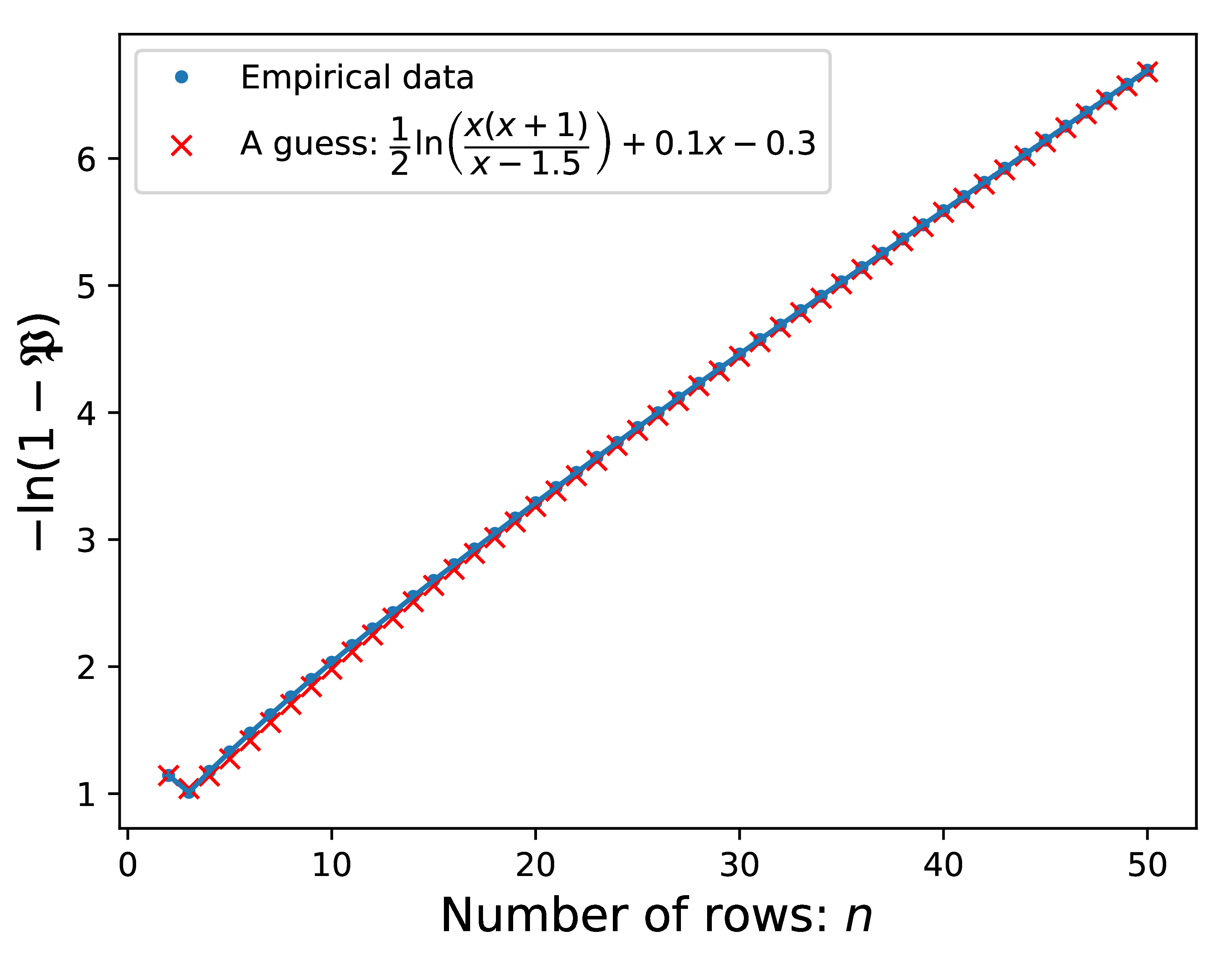
Refer to caption
Figure 8: A guess of the 𝔓𝔓\mathfrak{P} values for each n𝑛n together with empirical data

And we have an empirical formula to describe the relation between 𝔓𝔓\mathfrak{P} and n𝑛n, shown in Fig. 8:

𝔓(n,2)=1x1.5x(x+1)e0.1x+0.3subscript𝔓𝑛21𝑥1.5𝑥𝑥1superscript𝑒0.1𝑥0.3\mathfrak{P}_{(n,2)}=1-\sqrt{\dfrac{x-1.5}{x(x+1)}}e^{-0.1x+0.3} (45)

Appendix C Theory and Empirical Data on Stability

C.1 Proof of Proposition 5.1

Proposition C.1 (Proposition 5.1).

Given a sequence of identical independent 𝒟𝒟\mathcal{D}-valued random variables (Di)i1subscriptsubscriptD𝑖𝑖1(\mathrm{D}_{i})_{i\geq 1} following uniform distribution. Let μ0𝒫(Δm1)subscript𝜇0𝒫superscriptΔ𝑚1\mu_{0}\in\mathcal{P}(\Delta^{m-1}) be a prior distribution on Δm1superscriptΔ𝑚1\Delta^{m-1}, and μk+1=ΨDk𝐋(μk)subscript𝜇𝑘1superscriptsubscriptΨsubscriptD𝑘𝐋subscript𝜇𝑘\mu_{k+1}=\Psi_{\mathrm{D}_{k}}^{\mathbf{L}}(\mu_{k}), then μksubscript𝜇𝑘\mu_{k} converges, in probability, to iaiδisubscript𝑖subscript𝑎𝑖subscript𝛿𝑖\sum_{i\in\mathcal{H}}a_{i}\delta_{i}, where ai=𝔼μ0[θ(i)]subscript𝑎𝑖subscript𝔼subscript𝜇0delimited-[]𝜃𝑖a_{i}=\mathbb{E}_{\mu_{0}}\left[\theta(i)\right].

To show the above proposition, we need the following lemma:

Lemma C.1.1.

Given the conditions in Proposition C.1, then for any k𝑘k\in\mathbb{N} and hh\in\mathcal{H},

𝔼μk(θ(h))=𝔼μ0(θ(h)).subscript𝔼subscript𝜇𝑘𝜃subscript𝔼subscript𝜇0𝜃\mathbb{E}_{\mu_{k}}(\theta(h))=\mathbb{E}_{\mu_{0}}(\theta(h)). (46)
Proof.

It suffices to show 𝔼μk+1(θ(h))=𝔼μk(θ(h))subscript𝔼subscript𝜇𝑘1𝜃subscript𝔼subscript𝜇𝑘𝜃\mathbb{E}_{\mu_{k+1}}(\theta(h))=\mathbb{E}_{\mu_{k}}(\theta(h)) for any k𝑘k.

𝔼μk+1(θ(h))subscript𝔼subscript𝜇𝑘1𝜃\displaystyle\mathbb{E}_{\mu_{k+1}}(\theta(h)) =\displaystyle= Δm1θ(h)d(μk+1)(θ)subscriptsuperscriptΔ𝑚1𝜃dsubscript𝜇𝑘1𝜃\displaystyle\int_{\Delta^{m-1}}\theta(h)\mathrm{d}(\mu_{k+1})(\theta)
=\displaystyle= d𝒟Dk(d)Δm1Td(θ)(h)dμk(θ)subscript𝑑𝒟subscriptDk𝑑subscriptsuperscriptΔ𝑚1subscript𝑇𝑑𝜃differential-dsubscript𝜇𝑘𝜃\displaystyle\sum_{d\in\mathcal{D}}\mathrm{D_{k}}(d)\int_{\Delta^{m-1}}T_{d}(\theta)(h)\mathrm{d}\mu_{k}(\theta)
=\displaystyle= Δm11nd𝒟Td(θ)(h)d(μk)(θ)subscriptsuperscriptΔ𝑚11𝑛subscript𝑑𝒟subscript𝑇𝑑𝜃dsubscript𝜇𝑘𝜃\displaystyle\int_{\Delta^{m-1}}\dfrac{1}{n}\sum_{d\in\mathcal{D}}T_{d}(\theta)(h)\mathrm{d}(\mu_{k})(\theta)
=\displaystyle= Δm1θ(h)d(μk)(θ)=𝔼μk(θ(h)).subscriptsuperscriptΔ𝑚1𝜃dsubscript𝜇𝑘𝜃subscript𝔼subscript𝜇𝑘𝜃\displaystyle\int_{\Delta^{m-1}}\theta(h)\mathrm{d}(\mu_{k})(\theta)=\mathbb{E}_{\mu_{k}}(\theta(h)).

Proof of Proposition C.1.

We first show the following result:

For any ϵ>0italic-ϵ0\epsilon>0, let

Δϵ:={θΔm1:θ(i)1ϵ,i=1,2,,m},assignsubscriptΔitalic-ϵconditional-set𝜃superscriptΔ𝑚1formulae-sequence𝜃𝑖1italic-ϵfor-all𝑖12𝑚\Delta_{\epsilon}:=\left\{\theta\in\Delta^{m-1}:\theta(i)\leq 1-\epsilon,\forall i=1,2,\dots,m\right\},

then limkμk(Δϵ)=0subscript𝑘subscript𝜇𝑘subscriptΔitalic-ϵ0\lim\limits_{k\rightarrow\infty}\mu_{k}(\Delta_{\epsilon})=0.

We prove this by contradiction. Suppose the limit does not exist or is not 00, then there is a positive number C𝐶C and a subsequence (μki)isubscriptsubscript𝜇subscript𝑘𝑖𝑖(\mu_{k_{i}})_{i\in\mathbb{N}} such that μki(Δϵ)>Csubscript𝜇subscript𝑘𝑖subscriptΔitalic-ϵ𝐶\mu_{k_{i}}(\Delta_{\epsilon})>C for all i𝑖i.

We define a linear functional (μ):=𝔼μf(θ)assign𝜇subscript𝔼𝜇𝑓𝜃\mathscr{L}(\mu):=\mathbb{E}_{\mu}f(\theta), where f(θ)=θu22𝑓𝜃superscriptsubscriptnorm𝜃𝑢22f(\theta)=||\theta-u||_{2}^{2} with u=𝐞m𝑢𝐞𝑚u=\dfrac{\mathbf{e}}{m} the center of Δm1superscriptΔ𝑚1\Delta^{m-1}.

By definition, for a random variable following uniform distribution on 𝒟𝒟\mathcal{D}, (ΨD𝐋(μ))=𝔼μ(𝔼dDf(Td(θ)))superscriptsubscriptΨD𝐋𝜇subscript𝔼𝜇subscript𝔼similar-to𝑑D𝑓subscript𝑇𝑑𝜃\mathscr{L}\left(\Psi_{\mathrm{D}}^{\mathbf{L}}(\mu)\right)=\mathbb{E}_{\mu}\left(\mathbb{E}_{d\sim\mathrm{D}}f(T_{d}(\theta))\right).

Consider that f𝑓f is a strictly convex function, by Jensen’s inequality, 𝔼dDf(Td(θ))f(𝔼dDTd(θ))=f(θ)subscript𝔼similar-to𝑑D𝑓subscript𝑇𝑑𝜃𝑓subscript𝔼similar-to𝑑Dsubscript𝑇𝑑𝜃𝑓𝜃\mathbb{E}_{d\sim\mathrm{D}}f(T_{d}(\theta))\geq f(\mathbb{E}_{d\sim\mathrm{D}}T_{d}(\theta))=f(\theta), with equality if and only if Td(θ)=θsubscript𝑇𝑑𝜃𝜃T_{d}(\theta)=\theta for all d𝒟𝑑𝒟d\in\mathcal{D}, equivalently by the assumptions on matrix 𝐋𝐋\mathbf{L}, θ=δh𝜃subscript𝛿\theta=\delta_{h} for some hh\in\mathcal{H}. (This is because we assume 𝐋𝐋\mathbf{L} have distinct columns, thus not all 222-by-222 cross-ratios are 111, for any pair of columns. however, after Tdsubscript𝑇𝑑T_{d} all 222-by-222 cross-ratios are 111, indicating the existence of degeneration on every pair of columns. This can only happen when θ=δh𝜃subscript𝛿\theta=\delta_{h} for some hh\in\mathcal{H}.)

Thus for any θΔϵ𝜃subscriptΔitalic-ϵ\theta\in\Delta_{\epsilon}, 𝔼dDf(Td(θ))>f(θ)subscript𝔼similar-to𝑑D𝑓subscript𝑇𝑑𝜃𝑓𝜃\mathbb{E}_{d\sim\mathrm{D}}f(T_{d}(\theta))>f(\theta). As ΔϵsubscriptΔitalic-ϵ\Delta_{\epsilon} is compact, there is a lower bound B>0𝐵0B>0, such that 𝔼dDf(Td(θ))f(θ)>Bsubscript𝔼similar-to𝑑D𝑓subscript𝑇𝑑𝜃𝑓𝜃𝐵\mathbb{E}_{d\sim\mathrm{D}}f(T_{d}(\theta))-f(\theta)>B for all θΔϵ𝜃subscriptΔitalic-ϵ\theta\in\Delta_{\epsilon}. Thus

(μki+1)subscript𝜇subscript𝑘𝑖1\displaystyle\mathscr{L}(\mu_{k_{i}+1})
=\displaystyle= Δm1\Δϵ𝔼d𝒟f(Td(θ))dμki+Δϵ𝔼d𝒟f(Td(θ))dμkisubscript\superscriptΔ𝑚1subscriptΔitalic-ϵsubscript𝔼similar-to𝑑𝒟𝑓subscript𝑇𝑑𝜃differential-dsubscript𝜇subscript𝑘𝑖subscriptsubscriptΔitalic-ϵsubscript𝔼similar-to𝑑𝒟𝑓subscript𝑇𝑑𝜃differential-dsubscript𝜇subscript𝑘𝑖\displaystyle\!\!\!\!\!\int\limits_{\Delta^{m-1}\backslash\Delta_{\epsilon}}\!\!\!\mathbb{E}_{d\sim\mathcal{D}}f(T_{d}(\theta))\mathrm{d}\mu_{k_{i}}+\int\limits_{\Delta_{\epsilon}}\mathbb{E}_{d\sim\mathcal{D}}f(T_{d}(\theta))\mathrm{d}\mu_{k_{i}}
>\displaystyle> Δm1\Δϵf(θ)dμki+Δϵf(θ)dμki+BCsubscript\superscriptΔ𝑚1subscriptΔitalic-ϵ𝑓𝜃differential-dsubscript𝜇subscript𝑘𝑖subscriptsubscriptΔitalic-ϵ𝑓𝜃differential-dsubscript𝜇subscript𝑘𝑖𝐵𝐶\displaystyle\!\!\!\!\int\limits_{\Delta^{m-1}\backslash\Delta_{\epsilon}}\!\!f(\theta)\mathrm{d}\mu_{k_{i}}+\int\limits_{\Delta_{\epsilon}}f(\theta)\mathrm{d}\mu_{k_{i}}+BC
=\displaystyle= (μki)+BCsubscript𝜇subscript𝑘𝑖𝐵𝐶\displaystyle\mathscr{L}(\mu_{k_{i}})+BC

for all i𝑖i\in\mathbb{N} and simply (μk+1)(μk)subscript𝜇𝑘1subscript𝜇𝑘\mathscr{L}(\mu_{k+1})\geq\mathscr{L}(\mu_{k}) for general k𝑘k.

Therefore, (μk)subscript𝜇𝑘\mathscr{L}(\mu_{k}) is unbounded as k𝑘k\rightarrow\infty since there is at least a BC>0𝐵𝐶0BC>0 increment at each kisubscript𝑘𝑖k_{i}.

However, by definition, f𝑓f is bounded by m𝑚m since m𝑚\sqrt{m} is the diameter of Δm1superscriptΔ𝑚1\Delta^{m-1} under 222-norm, thus (μ)m𝜇𝑚\mathscr{L}(\mu)\leq m.

Such a contradiction shows that the opposite of our assumption, limkμk(Δϵ)=0subscript𝑘subscript𝜇𝑘subscriptΔitalic-ϵ0\lim\limits_{k\rightarrow\infty}\mu_{k}(\Delta_{\epsilon})=0, is valid.

Consider that ϵitalic-ϵ\epsilon is arbitrary, and in Lemma C.1.1 we show that 𝔼μkθ(h)subscript𝔼subscript𝜇𝑘𝜃\mathbb{E}_{\mu_{k}}\theta(h) is invariant, thus μksubscript𝜇𝑘\mu_{k} approaches iaiδisubscript𝑖subscript𝑎𝑖subscript𝛿𝑖\sum_{i\in\mathcal{H}}a_{i}\delta_{i} with ai=𝔼μ0θ(i)subscript𝑎𝑖subscript𝔼subscript𝜇0𝜃𝑖a_{i}=\mathbb{E}_{\mu_{0}}\theta(i) in probability. ∎

C.2 Empirical Data for Stability: Perturbation on Prior

We sample 555 matrices of size 3×3333\times 3, each of them are column-normalized, and their columns are sampled independently and uniformly on Δ2superscriptΔ2\Delta^{2}, listed below:

𝐌1subscript𝐌1\displaystyle\mathbf{M}_{1} =\displaystyle= (0.65590.55050.73100.16800.33590.04030.17600.11360.2287)0.65590.55050.73100.16800.33590.04030.17600.11360.2287\displaystyle\left(\begin{array}[]{ccc}0.6559&0.5505&0.7310\\ 0.1680&0.3359&0.0403\\ 0.1760&0.1136&0.2287\end{array}\right) (50)
𝐌2subscript𝐌2\displaystyle\mathbf{M}_{2} =\displaystyle= (0.24610.66000.43100.67850.06550.23250.07540.27460.3365)0.24610.66000.43100.67850.06550.23250.07540.27460.3365\displaystyle\left(\begin{array}[]{ccc}0.2461&0.6600&0.4310\\ 0.6785&0.0655&0.2325\\ 0.0754&0.2746&0.3365\end{array}\right) (54)
𝐌3subscript𝐌3\displaystyle\mathbf{M}_{3} =\displaystyle= (0.72860.19370.76200.07390.47860.19990.19740.32770.0382)0.72860.19370.76200.07390.47860.19990.19740.32770.0382\displaystyle\left(\begin{array}[]{ccc}0.7286&0.1937&0.7620\\ 0.0739&0.4786&0.1999\\ 0.1974&0.3277&0.0382\end{array}\right) (58)
𝐌4subscript𝐌4\displaystyle\mathbf{M}_{4} =\displaystyle= (0.47450.20240.59460.28980.74990.13130.23570.04770.2741)0.47450.20240.59460.28980.74990.13130.23570.04770.2741\displaystyle\left(\begin{array}[]{ccc}0.4745&0.2024&0.5946\\ 0.2898&0.7499&0.1313\\ 0.2357&0.0477&0.2741\end{array}\right) (62)
𝐌5subscript𝐌5\displaystyle\mathbf{M}_{5} =\displaystyle= (0.22070.54660.16050.38280.38070.56970.39650.07270.2698)0.22070.54660.16050.38280.38070.56970.39650.07270.2698\displaystyle\left(\begin{array}[]{ccc}0.2207&0.5466&0.1605\\ 0.3828&0.3807&0.5697\\ 0.3965&0.0727&0.2698\end{array}\right) (66)

And the 555 sampled priors are:

θ1subscript𝜃1\displaystyle\theta_{1} =\displaystyle= (0.3333,0.3333,0.3333)superscript0.33330.33330.3333top\displaystyle\left(0.3333,0.3333,0.3333\right)^{\top}
θ2subscript𝜃2\displaystyle\theta_{2} =\displaystyle= (0.1937,0.4291,0.3771)superscript0.19370.42910.3771top\displaystyle\left(0.1937,0.4291,0.3771\right)^{\top}
θ3subscript𝜃3\displaystyle\theta_{3} =\displaystyle= (0.4544,0.0814,0.4641)superscript0.45440.08140.4641top\displaystyle\left(0.4544,0.0814,0.4641\right)^{\top}
θ4subscript𝜃4\displaystyle\theta_{4} =\displaystyle= (0.5955,0.2995,0.1051)superscript0.59550.29950.1051top\displaystyle\left(0.5955,0.2995,0.1051\right)^{\top}
θ5subscript𝜃5\displaystyle\theta_{5} =\displaystyle= (0.4771,0.0593,0.4636)superscript0.47710.05930.4636top\displaystyle\left(0.4771,0.0593,0.4636\right)^{\top} (67)

These names (including the rank 444 samples below) are overriding the previously defined identical symbols in this part and in the corresponding subsection in the main paper. In the 4×4444\times 4 cases, we sample 333 matrices in the same way as in 3×3333\times 3 case.

𝐌1superscriptsubscript𝐌1\displaystyle\mathbf{M}_{1}^{\prime}\!\! =\displaystyle= (0.39160.23060.04600.04040.14080.63500.21390.23100.23750.02750.16670.24120.23010.10680.57340.4874)0.39160.23060.04600.04040.14080.63500.21390.23100.23750.02750.16670.24120.23010.10680.57340.4874\displaystyle\!\!\left(\begin{array}[]{cccc}0.3916&0.2306&0.0460&0.0404\\ 0.1408&0.6350&0.2139&0.2310\\ 0.2375&0.0275&0.1667&0.2412\\ 0.2301&0.1068&0.5734&0.4874\end{array}\right) (72)
𝐌2superscriptsubscript𝐌2\displaystyle\mathbf{M}_{2}^{\prime}\!\! =\displaystyle= (0.37440.68920.01120.32000.32040.23200.44980.35300.02910.06880.38650.06530.27610.01000.15260.2618)0.37440.68920.01120.32000.32040.23200.44980.35300.02910.06880.38650.06530.27610.01000.15260.2618\displaystyle\!\!\left(\begin{array}[]{cccc}0.3744&0.6892&0.0112&0.3200\\ 0.3204&0.2320&0.4498&0.3530\\ 0.0291&0.0688&0.3865&0.0653\\ 0.2761&0.0100&0.1526&0.2618\end{array}\right) (77)
𝐌3superscriptsubscript𝐌3\displaystyle\mathbf{M}_{3}^{\prime}\!\! =\displaystyle= (0.28850.08730.23190.10090.06530.22390.05750.25840.59340.32760.22830.39250.05290.36120.48230.2482)0.28850.08730.23190.10090.06530.22390.05750.25840.59340.32760.22830.39250.05290.36120.48230.2482\displaystyle\!\!\left(\begin{array}[]{cccc}0.2885&0.0873&0.2319&0.1009\\ 0.0653&0.2239&0.0575&0.2584\\ 0.5934&0.3276&0.2283&0.3925\\ 0.0529&0.3612&0.4823&0.2482\end{array}\right) (82)

And 333 corresponding priors are sampled:

θ1superscriptsubscript𝜃1\displaystyle\theta_{1}^{\prime} =\displaystyle= (0.2500,0.2500,0.2500,0.2500)superscript0.25000.25000.25000.2500top\displaystyle\left(0.2500,0.2500,0.2500,0.2500\right)^{\top}
θ2superscriptsubscript𝜃2\displaystyle\theta_{2}^{\prime} =\displaystyle= (0.1789,0.3664,0.2915,0.1632)superscript0.17890.36640.29150.1632top\displaystyle\left(0.1789,0.3664,0.2915,0.1632\right)^{\top}
θ3superscriptsubscript𝜃3\displaystyle\theta_{3}^{\prime} =\displaystyle= (0.4460,0.4676,0.0821,0.0043)superscript0.44600.46760.08210.0043top\displaystyle\left(0.4460,0.4676,0.0821,0.0043\right)^{\top} (83)
Refer to caption
Figure 9: Successful rate of SCBI perturbed on prior. Each entry corresponds to a pair 𝐌𝐌\mathbf{M} and θ0Tsuperscriptsubscript𝜃0𝑇\theta_{0}^{T}. The first row shows for each prior θ0Tsuperscriptsubscript𝜃0𝑇\theta_{0}^{T}, the position it locates in Δ2superscriptΔ2\Delta^{2} and the range of θ0Lsuperscriptsubscript𝜃0𝐿\theta_{0}^{L} in the simulation. The 555 rows below are the zoom-in version of the shaded area in each case, whose color at each point represents the successful rate when θ0Lsuperscriptsubscript𝜃0𝐿\theta_{0}^{L} locates at that point.

The value we use to test the effectiveness of perturbed SCBI is called the successful rate, which is 𝔼[θL(h)]=𝔼μL[θ(h)]𝔼delimited-[]superscriptsubscript𝜃𝐿subscript𝔼superscriptsubscript𝜇𝐿delimited-[]𝜃\mathbb{E}\left[\theta_{\infty}^{L}(h)\right]=\mathbb{E}_{\mu_{\infty}^{L}}\left[\theta(h)\right] where hh is the true hypothesis that the teacher teaches (Definition 5.2). Successful rate is well defined, i.e. the limit exists, according to the convergences in probability (Theorem A.3 and Proposition C.1) with an ϵitalic-ϵ\epsilon discussion based on them. To find the successful rate, we use Monte-Carlo method on 104superscript10410^{4} teaching sequences, and use Proposition C.1 to accelerate the simulation.

We can estimate an upper bound of the standard deviation (precision) of the empirical successful rate calculated based on Proposition C.1. The successful rate of a single teaching sequence is between 00 and 111, thus with a standard deviation smaller than 111. So the standard deviation of the empirical successful rate is bounded by (N)1/2superscript𝑁12(N)^{-1/2} where N𝑁N is the number of sample sequences. Actually the precision is much smaller since the successful rate for a single sequence is much more stable.

Our first simulation is shown in Fig. 9, where we take θ0Lsuperscriptsubscript𝜃0𝐿\theta_{0}^{L} evenly on a series of concentric circles centered at θ0Tsuperscriptsubscript𝜃0𝑇\theta_{0}^{T}. There are 141414 such circles with radius 0.0050.0050.005 to 0.070.070.07. On the i𝑖i-th layer (smallest circle is the first layer) we take 6i6𝑖6i many points evenly separated, the upper right figure in Fig. 10 shows how the points are taken in detail.

Thus we have 666 groups of points each distributed along a ray. We plot the successful rate versus the distance from the center along each ray in Fig. 10 for all the 252525 combinations of 𝐌𝐌\mathbf{M} and θ0Tsuperscriptsubscript𝜃0𝑇\theta_{0}^{T}.

Refer to caption
Refer to caption
Refer to caption
Figure 10: Upper-Left: the six rays at the center θ1subscript𝜃1\theta_{1}. Upper-Right: zoom-in figure of the six rays in general. Lower: Successful rate versus distance to center along 666 rays. Fig. 5 in the main paper contains the Row 3 Column 1 picture of the lower one (with a different y𝑦y-scale).

To have a similar directional data for matrices of size 4×4444\times 4, we take a sample of 151515 directions in 3superscript3\mathbb{R}^{3} (showing in Fig. 11 in spherical coordinates centered at (1/4,1/4,1/4,1/4)superscript14141414top(1/4,1/4,1/4,1/4)^{\top}, with (1,0,0,0)superscript1000top(1,0,0,0)^{\top} as ϕ=0italic-ϕ0\phi=0 axis and (0,1,0,0)superscript0100top(0,1,0,0)^{\top} on the half-plane given by θ=0𝜃0\theta=0) and simulate the perturbations of θ0Lsuperscriptsubscript𝜃0𝐿\theta_{0}^{L} in Δ3superscriptΔ3\Delta^{3} along the 151515 directions. On each ray, we take 202020 evenly placed θ0Lsuperscriptsubscript𝜃0𝐿\theta_{0}^{L} with distance to the center θ0Tsuperscriptsubscript𝜃0𝑇\theta_{0}^{T} from 0.0050.0050.005 to 0.1000.1000.100. Then we plot the successful rate versus the distance in Fig. 11 for all 999 cases as before.

Refer to caption
Refer to caption
Figure 11: Upper: the sampled directions in spherical coordinates. Lower: Successful rate versus distance to center, along 15 rays, for all the 999 cases of matrices of size 4×4444\times 4. The plot at Row 1 Column 1 appears in Fig. 5 of the main file.
Remark 7.

This part provides evidences of linear influence of the perturbation distance on the successful rate along a fixed direction.

Next we explore the global behavior of perturbations on prior. Here we sample for each combination of 𝐌𝐌\mathbf{M} and θ0Tsuperscriptsubscript𝜃0𝑇\theta_{0}^{T} a set of 300300300 points for θ0Lsuperscriptsubscript𝜃0𝐿\theta_{0}^{L} evenly distributed in Δ3superscriptΔ3\Delta^{3}.

In Fig. 12, we plot the successful rate versus the value of θ0L(h)superscriptsubscript𝜃0𝐿\theta_{0}^{L}(h), for all 252525 situations.

Refer to caption
Figure 12: The 25 cases of 3×3333\times 3 matrices, with successful rate versus θ0T(h)superscriptsubscript𝜃0𝑇\theta_{0}^{T}(h) plotted. Plot at Row 3 Column 1 appears in Fig. 5 of the main file.

We plot in Fig. 13 the distance to center as x𝑥x-coordinates, for 999 situations with matrices of size 4×4444\times 4.

Refer to caption
Figure 13: The 9 cases of 4×4444\times 4 matrices, with successful rate versus the distance to the center plotted. Plot at Row 1 Column 1 appears in Fig. 5 of the main file. Red line is the lower bound given in Conjecture 5.3.

In this part, we observe that there is a lower bound of the successful rate which depends linearly on the distance to center, with slope bounded by 1θ0T(h)1superscriptsubscript𝜃0𝑇\frac{1}{\theta_{0}^{T}(h)} (Conjecture 5.3).

C.3 Empirical Data for Stability: Perturbation on Matrix

Fig. 14 shows the behavior of perturbations on all sampled 3×3333\times 3 matrices in Section 5. Perturbations are taken only along the relevant column / irrelevant column, since a perturbation on the target column is equivalent of the combination of a perturbation on other two columns (they have the same set of Cross-ratios, which determines the SCBI behavior). The cycle path in each plot is the equi-normalized-KL path, with any point on the path having the same normalized-KL to the target column as that of the original matrix 𝐓𝐓\mathbf{T}.

These graphs should not be confused with the ones occur in the prior perturbed part, as we are plotting each column of the matrix here (the simplex is actually 𝒫(𝒟)𝒫𝒟\mathcal{P}(\mathcal{D})), while we were plotting the priors in previous discussion (the simplex is 𝒫()𝒫\mathcal{P}(\mathcal{H})).

Refer to caption
Refer to caption
Refer to caption
Refer to caption
Refer to caption
Refer to caption
Refer to caption
Refer to caption
Refer to caption
Refer to caption
Refer to caption
Refer to caption
Refer to caption
Refer to caption
Refer to caption
Refer to caption
Refer to caption
Refer to caption
Refer to caption
Refer to caption
Figure 14: Perturbations on matrix 𝐋𝐋\mathbf{L}. First column: Perturbations on the irrelevant column of 𝐋𝐋\mathbf{L}. Second column: zoom-in of the first row. Third column: Perturbations on the relevant column of 𝐋𝐋\mathbf{L}. Last column: zoom-in of the third column. The scales of color in the zoomed figures are different from that of the original ones. Fig. 6 in the main paper is the third row here.

Acknowledgements

This material is based on research sponsored by the Air Force Research Laboratory and DARPA under agreement number FA8750-17-2-0146 and the Army Research Office and DARPA under agreement HR00112020039. The U.S. Government is authorized to reproduce and distribute reprints for Governmental purposes notwithstanding any copyright notation thereon. This work was also supported by DoD grant 72531RTREP and NSF MRI 1828528 to PS.

References

  • Bengio et al. (2009) Bengio, Y., Louradour, J., Collobert, R., and Weston, J. Curriculum learning. In Proceedings of the 26th annual international conference on machine learning, pp.  41–48. ACM, 2009.
  • Berger et al. (1994) Berger, J. O., Moreno, E., Pericchi, L. R., Bayarri, M. J., Bernardo, J. M., Cano, J. A., De la Horra, J., Martín, J., Ríos-Insúa, D., Betrò, B., et al. An overview of robust bayesian analysis. Test, 3(1):5–124, 1994.
  • Bonawitz et al. (2011) Bonawitz, E., Shafto, P., Gweon, H., Goodman, N. D., Spelke, E., and Schulz, L. The double-edged sword of pedagogy: Instruction limits spontaneous exploration and discovery. Cognition, 120(3):322–330, 2011.
  • Bridgers et al. (in press) Bridgers, S., Jara-Ettinger, J., and Gweon, H. Young children consider the expected utility of others’ learning to decide what to teachn. Nature Human Behaviour, in press.
  • Csibra & Gergely (2009) Csibra, G. and Gergely, G. Natural pedagogy. Trends in cognitive sciences, 13(4):148–153, 2009.
  • Doliwa et al. (2014) Doliwa, T., Fan, G., Simon, H. U., and Zilles, S. Recursive teaching dimension, VC-dimension and sample compression. Journal of Machine Learning Research, 15(1):3107–3131, 2014.
  • Doob (1949) Doob, J. L. Application of the theory of martingales. Le calcul des probabilites et ses applications, pp.  23–27, 1949.
  • Eaves & Shafto (2016) Eaves, B. S. and Shafto, P. Parameterizing developmental changes in epistemic trust. Psychonomic Bulletin & Review, pp.  1–30, 2016.
  • Eaves Jr et al. (2016) Eaves Jr, B. S., Feldman, N. H., Griffiths, T. L., and Shafto, P. Infant-directed speech is consistent with teaching. Psychological review, 123(6):758, 2016.
  • Elman (1993) Elman, J. L. Learning and development in neural networks: The importance of starting small. Cognition, 48(1):71–99, 1993.
  • Fienberg et al. (1970) Fienberg, S. E. et al. An iterative procedure for estimation in contingency tables. The Annals of Mathematical Statistics, 41(3):907–917, 1970.
  • Fisac et al. (2017) Fisac, J. F., Gates, M. A., Hamrick, J. B., Liu, C., Hadfield-Menell, D., Palaniappan, M., Malik, D., Sastry, S. S., Griffiths, T. L., and Dragan, A. D. Pragmatic-pedagogic value alignment. arXiv preprint arXiv:1707.06354, 2017.
  • Frank & Goodman (2012) Frank, M. C. and Goodman, N. D. Predicting pragmatic reasoning in language games. Science, 336(6084):998–998, 2012.
  • Ghahramani (2015) Ghahramani, Z. Probabilistic machine learning and artificial intelligence. Nature, 521(7553):452, 2015.
  • Goodman & Stuhlmüller (2013) Goodman, N. D. and Stuhlmüller, A. Knowledge and implicature: Modeling language understanding as social cognition. Topics in cognitive science, 5(1):173–184, 2013.
  • Hadfield-Menell et al. (2016) Hadfield-Menell, D., Russell, S. J., Abbeel, P., and Dragan, A. Cooperative inverse reinforcement learning. In Advances in neural information processing systems, pp. 3909–3917, 2016.
  • Hershkowitz et al. (1988) Hershkowitz, D., Rothblum, U. G., and Schneider, H. Classifications of nonnegative matrices using diagonal equivalence. SIAM journal on Matrix Analysis and Applications, 9(4):455–460, 1988.
  • Ho et al. (2016) Ho, M. K., Littman, M., MacGlashan, J., Cushman, F., and Austerweil, J. L. Showing versus doing: Teaching by demonstration. In Advances in Neural Information Processing Systems, pp. 3027–3035, 2016.
  • Jara-Ettinger et al. (2016) Jara-Ettinger, J., Gweon, H., Schulz, L. E., and Tenenbaum, J. B. The naïve utility calculus: Computational principles underlying commonsense psychology. Trends in cognitive sciences, 20(8):589–604, 2016.
  • Kadane et al. (1978) Kadane, J. B., Chuang, D. T., et al. Stable decision problems. The Annals of Statistics, 6(5):1095–1110, 1978.
  • Miescke & Liese (2008) Miescke, K.-J. and Liese, F. Statistical Decision Theory: Estimation, Testing, and Selection. Springer, 2008. doi: https://doi.org/10.1007/978-0-387-73194-0.
  • Murphy (2012) Murphy, K. P. Machine learning: a probabilistic perspective. MIT press, 2012.
  • Schneider (1989) Schneider, M. H. Matrix scaling, entropy minimization, and conjugate duality. i. existence conditions. Linear Algebra and its Applications, 114:785–813, 1989.
  • Shafto & Goodman (2008) Shafto, P. and Goodman, N. Teaching games: Statistical sampling assumptions for learning in pedagogical situations. In Proceedings of the 30th annual conference of the Cognitive Science Society, pp.  1632–1637. Cognitive Science Society Austin, TX, 2008.
  • Shafto et al. (2012) Shafto, P., Goodman, N. D., and Frank, M. C. Learning from others: The consequences of psychological reasoning for human learning. Perspectives on Psychological Science, 7(4):341–351, 2012.
  • Shafto et al. (2014) Shafto, P., Goodman, N. D., and Griffiths, T. L. A rational account of pedagogical reasoning: Teaching by, and learning from, examples. Cognitive Psychology, 71:55–89, 2014.
  • Skinner (1958) Skinner, B. F. Teaching machines. Science, 128(3330):969–977, 1958.
  • Tenenbaum et al. (2011) Tenenbaum, J. B., Kemp, C., Griffiths, T. L., and Goodman, N. D. How to grow a mind: Statistics, structure, and abstraction. science, 331(6022):1279–1285, 2011.
  • Tomasello (1999) Tomasello, M. The cultural origins of human cognition. Harvard University Press, Cambridge, MA, 1999.
  • Wang et al. (2019a) Wang, P., Paranamana, P., and Shafto, P. Generalizing the theory of cooperative inference. AIStats, 2019a.
  • Wang et al. (2019b) Wang, P., Wang, J., Paranamana, P., and Shafto, P. A mathematical theory of cooperative communication, 2019b.
  • Yang et al. (2018) Yang, S. C., Yu, Y., Givchi, A., Wang, P., Vong, W. K., and Shafto, P. Optimal cooperative inference. In AISTATS, volume 84 of Proceedings of Machine Learning Research, pp.  376–385. PMLR, 2018.
  • Zhu (2013) Zhu, X. Machine teaching for bayesian learners in the exponential family. In Advances in Neural Information Processing Systems, pp. 1905–1913, 2013.
  • Zhu (2015) Zhu, X. Machine teaching: An inverse problem to machine learning and an approach toward optimal education. In AAAI, pp.  4083–4087, 2015.
  • Zilles et al. (2008) Zilles, S., Lange, S., Holte, R., and Zinkevich, M. Teaching dimensions based on cooperative learning. In COLT, pp.  135–146, 2008.