The QCD crossover at finite chemical potential from lattice simulations
Abstract
We provide the most accurate results for the QCD transition line so far. We optimize the definition of the crossover temperature , allowing for its very precise determination, and extrapolate from imaginary chemical potential up to real MeV. The definition of adopted in this work is based on the observation that the chiral susceptibility as a function of the condensate is an almost universal curve at zero and imaganiary . We obtain the parameters and as a continuum extrapolation based on and lattices with physical quark masses. We also extrapolate the peak value of the chiral susceptibility and the width of the chiral transition along the crossover line. In fact, both of these are consistent with a constant function of . We see no sign of criticality in the explored range.
Introduction— One of the most important open problems in the study of Quantum Chromodynamics (QCD) at finite temperature and density is the determination of the phase diagram of the theory in the temperature ()-baryo-chemical potential () plane. It is now established by first principle lattice QCD calculations that the transition at is a smooth crossover Aoki et al. (2006a); Bhattacharya et al. (2014) for physical quark masses. Due to the lack of a real phase transition, the crossover temperature is of course ambiguous, since different definitions can lead to different values for it. Observables related to chiral symmetry (i.e. the chiral condensate and its susceptibility) yield a transition temperature around MeV Aoki et al. (2006b, 2009); Borsanyi et al. (2010); Bazavov et al. (2012).
Extending our knowledge to the part of the phase diagram turns out to be very challenging, due to the notorious sign problem. Since this makes direct simulation at finite impossible, the state-of-the-art for finite density QCD on fine lattices is to use one of two extrapolation methods. The first method is the direct calculation of Taylor coefficients Allton et al. (2002, 2005); Gavai and Gupta (2008); Basak et al. (2008); Borsanyi et al. (2012a, b); Bellwied et al. (2015a); Ding et al. (2015); Bazavov et al. (2017, 2018, 2020) using simulations at , while the second is to use simulations at imaginary chemical potentials () where the sign problem is absent, and later perform an extrapolation of different quantities to a real chemical potential () de Forcrand and Philipsen (2002); D’Elia and Lombardo (2003); D’Elia and Sanfilippo (2009); Cea et al. (2014); Bonati et al. (2014); Cea et al. (2016); Bonati et al. (2015); Bellwied et al. (2015b); D’Elia et al. (2017); Gunther et al. (2017); Alba et al. (2017); Vovchenko et al. (2017); Bonati et al. (2018); Borsanyi et al. (2018). It is often conjectured that in the plane the crossover line, departing from , eventually turns into a first-order transition line. The point separating the crossover and the first-order transitions is known as the critical endpoint (CEP), where the transition is expected to be of second order. Though there have been attempts in extracting information about the location of the supposed CEP from lattice simulations Fodor and Katz (2002, 2004); D’Elia et al. (2017); Bazavov et al. (2017); Fodor et al. (2019); Giordano and Psztor (2019); Mukherjee and Skokov (2019); Giordano et al. (2019), these attempts face great difficulties, as extrapolation-type methods have the property that they give reliable results mostly in the immediate vicinity of .
In this letter, we address the problem of calculating the Taylor coefficients of the crossover temperature around , parametrized as:
| (1) |
along the phenomenologically relevant strangeness neutrality line. In this work we improve the uncertainty on available in the literature Bazavov et al. (2018) by a factor of , giving a state-of-the-art determination of the cross-over line in the plane. In particular, as we will show, at chemical potentials the error on the extrapolation is dominated by the sub-leading coefficients e.g. . The coefficients and can be calculated with either one of the standard extrapolation methods. A direct evaluation of the derivatives from ensembles was used in Refs. Kaczmarek et al. (2011); Endrodi et al. (2011). The current state-of-the art using the simulation method is Ref. Bazavov et al. (2018), which includes the first continuum extrapolated results for . Here we will employ an analytical continuation from imaginary instead, and use lattices as fine as . This is motivated by the fact that the signal/noise ratio of higher derivatives is suppressed with powers of the lattice volume, therefore the calculation of higher order derivatives requires very high statistics. Determinations of using the imaginary method with continuum extrapolation include Refs. Bonati et al. (2015); Bellwied et al. (2015b). Finally, in Ref. Bonati et al. (2018) the two methods were compared with a careful check of the systematics, and a very good agreement was found for the coefficient .
We also study the strength of the crossover by extrapolating the width of the transition and the value of the chiral susceptibility at the transition to real in the continuum limit. While one always has to be careful not to over-interpret results from extrapolations, we currently do not see any sign of criticality up to MeV, as the crossover transition does not get narrower or stronger in this region.
On chiral observables in the transition region.— For the lattice simulations we use 4-stout improved staggered fermions with an aspect ratio of and temporal lattice sizes of . The details of the simulation setup can be found in the supplemental material.
The main observables in this study are the renormalized dimensionless chiral condensate and susceptibility, respectively defined as:
| (2) | ||||
where we assumed isospin symmetry, i.e. . In the above equations, the subscripts indicate values at finite- and zero-temperature, respectively. In the following, and are always shown after applying the correction to satisfy with zero statistical error (see the supplemental material for details). The peak height of the susceptibility is an indicator for the strength of the transition, while the peak position in temperature serves as a definition for the chiral cross-over temperature. It was pointed out in Refs. Aoki et al. (2006b, 2009) that different normalizations of the susceptibility, such as using or to define in Eq. (2) can shift the peak position by 11 MeV. This difference could be considered as a measure for the broadness of the chiral transition.
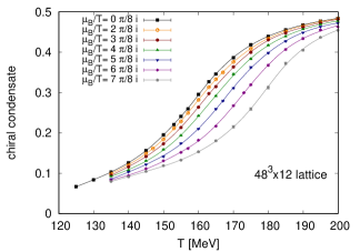
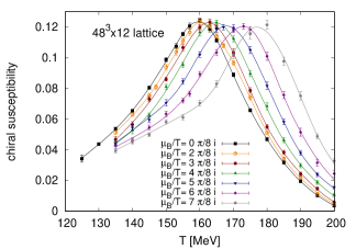
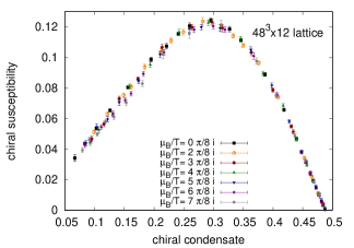
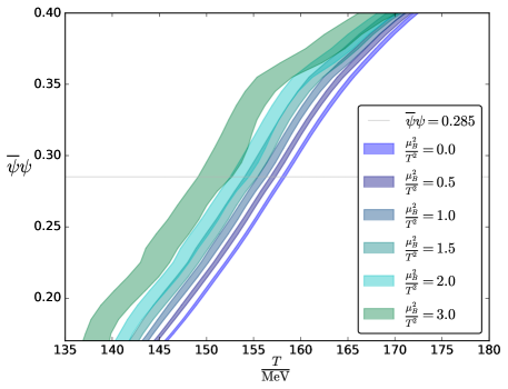
Our normalization choice in Eq. (2) was motivated by two observations, shown in Fig. 1 and explained below. These observations (together with the improved statistics and the more accurate tuning of to ) allow a very precise determination of as a function of imaginary chemical potential, which in turn allows a precise determination of the parameters and . We explored the chiral condensate and susceptibility in a broad range of imaginary baryo-chemical potential. In all panels of Fig. 1, the black curves correspond to . In the left and middle panel we show the chiral condensate and susceptibility as functions of the temperature. By construction, our renormalized condensate is zero at and positive at high temperature, because of the explicit vacuum subtraction and the overall negative sign in Eq. (2). In both panels, one can observe the shifting of the transition towards higher temperatures when an imaginary chemical potential is introduced. In the right panel we show the susceptibility as a function of the condensate. Here we converted the statistical error on the condensate into an additional error on the susceptibility, by solving for and substituting the resulting into (also taking the correlation of the statistical errors into account). Our first observation on the right panel of Fig. 1 is that the form of the curve is simpler than that of : a low (e.g. third or fourth) order polynomial can fit the entire transition range with an excellent fit quality. The second observation is that there is virtually no chemical potential dependence in the function. This way the susceptibility can be modeled as a low order polynomial of two variables, and . Had we used a different normalization for the susceptibility, e.g. as we did in Ref. Borsanyi et al. (2010), the peak height would be strongly -dependent and the collapse of the curves at different (imaginary) chemical potentials would not happen.
The transition line and its analytical continuation.— Keeping the previous observations in mind, one can perform a precise determination of , as defined by the peak of in Eq. (2) for various values of the imaginary chemical potential. can then be fitted for the coefficients and . This requires the following steps:
-
i)
Determine the renormalized condensate and susceptibility in a two-dimensional parameter scan in and using lattice simulations. Use these to obtain the susceptibility as a function of the condensate.
-
ii)
Search for the peak of through a low-order polynomial fit for each and obtaining .
-
iii)
Use an interpolation of to convert the to for each .
-
iv)
Perform a global fit of to determine the coefficients and for . For this step we use various functions – all containing an independent – with coefficients depending linearly on . The choice of the fit functions is motivated by the mock data analysis presented in the supplemental material.
The total systematic error comes from a pool of analyses: in step i) we have two choices for the scale setting, two choices for the renormalization of and two for the renormalization of ; in step ii) we use two choices for the fit function used to obtain the maximum of and two choices for the fit range; in step iii) we use two different interpolations of ; in step iv) we use two global fit functions and two choices for the range in . This leads to a total of ways to analyze our lattice data. These results are combined with a uniform weight. More details on the analyses, the fit qualities and the error estimates can be found in the supplemental material. We finally obtain:
| (3) | ||||||
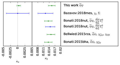
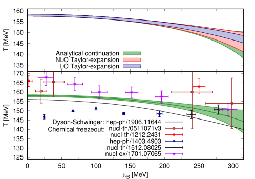
We stress that the uncertainties on these two quantities are correlated. We put these results in the context of previous lattice studies in Fig. 2. The extrapolated value of is shown in Fig. 3 (green band). Note that the errors on and are dominated by the statistical errors, as shown in the detailed discussion of the systematic error estimate in the supplemental material.
Since Ref. Bellwied et al. (2015b) we have more than doubled the statistics and introduced a more precise analysis. The overall error on has reduced slightly. The main result is the extraction of . It appears to be a generic feature of deducing Taylor-coefficients from polynomial fits: the increased precision on the input data leads to a sensitivity to a higher order coefficient first, and only later to a reduction of the error of both coefficients. This feature is also clearly seen in the mock data analysis in the supplemental material.
In Fig. 3 we also show the comparison to the leading order Taylor expansion result (using only ) and the next to leading order result (using and ). The latter is very close to our full result (for ), while the leading order result has a much smaller uncertainty. Clearly, is precise enough. At intermediate the bottleneck for the precision of is the error on . We also fitted , this turned out to be small enough to be irrelevant for .
Extrapolation of the transition width and strength.— A natural definition of the width of the susceptibility peak is given by its second derivative at as . Unfortunately, evaluating this quantity is numerically difficult, so we introduce a simple width parameter as a proxy for via:
| (4) |
with and . The choice of the range in is such that it is consistent with a linear behavior within our errorbars, meaning that the ratio can be used as a proxy for as well. The exact range in is chosen such that coincides with at zero and imaginary . A more detailed discussion of the width parameter can be found in the supplemental material.
We can define, for any value of , the temperature function
| (5) |
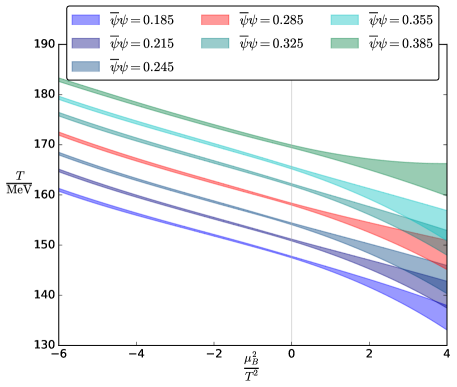
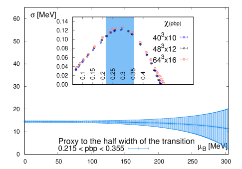
In the left panel of Fig. 4 we show these contours in the plane for a selection of values. We show continuum extrapolations and include the systematic errors. For this analysis the chiral susceptibility plays no role, since we use the same interpolations of as in step iii) of the analysis of the transition line, and two-dimensional fits (continuum and in ) analogous to those in step iv). We conclude that the half width of the transition – shown in the upper panel of Fig. 5 – is consistent with a constant up to within the uncertainty from the extrapolation (we note that uncertainty is reached at MeV). We also show as a function of for several fixed values of real in the right panel of Fig. 4, as extrapolated using the contours in the left panel of the same Figure.
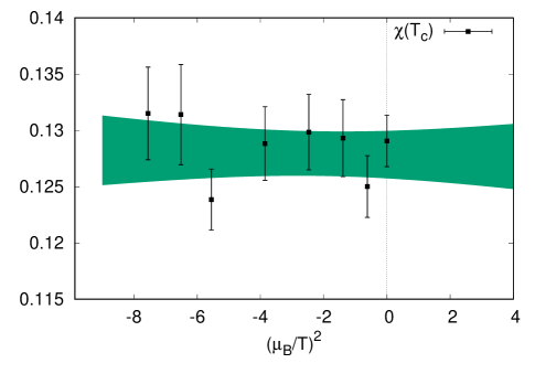
Finally, as a proxy for the strength of the crossover, we study the value of the chiral susceptibility at the crossover temperature. We get this for each and as a byproduct of steps i-ii) of the analysis for and . If one then performs a continuum extrapolation of the resulting values for fixed values of , one gets the lower panel of Fig. 5. Again, we see a very mild dependence, consistent with a constant.
Summary and discussion.— The main result of this work is a precise determination of the parameters and of the crossover line in finite density QCD. For the determination of the crossover line, we used the experimentally relevant tuned to keep . Based on the observation that the chiral susceptibility as a function of the condensate is a rather simple function, only weakly dependent on the imaginary chemical potential, we were able to obtain the transition temperature as a function of the imaginary chemical potential to very high accuracy. These pure lattice results can be used for further model building, and are summarized in the supplemental material. The high precision data at imaginary in turn allowed us to fit the and Taylor coefficients of the crossover temperature, and . In particular, while our determination of is still consistent with zero, the error is 6 times smaller than the one previously available in the literature, and therefore represents the state-of-the-art in the study of the phase diagram in the plane with current lattice techniques. As a byproduct, we also obtain the most precise value for the central temperature of the crossover at so far, as well as the width of the transition:
| (6) | |||||||||
The present definition was actually included in our earlier list of observables with Aoki et al. (2009). Recently the HotQCD collaboration has published for the peak of the chiral susceptibility in Ref. Bazavov et al. (2018).
Note that all results in this letter were obtained at a fixed aspect ratio of . Though this result is consistenct with earlier works, also with , finite volume corrections can potentially be relevant with the achieved precision. We also did not take into account isospin breaking and QED effects.
We also studied the strength of the phase transition as a function of by extrapolating our proxy for the transition width and the peak of the chiral susceptibility from imaginary chemical potentials. Even though one has to be careful with extrapolations, we see no sign of the transition getting stronger up to MeV.
Acknowledgements.— This project was funded by the DFG grant SFB/TR55. The project also received support from the BMBF Grant No. 05P18PXFCA. This work was also supported by the Hungarian National Research, Development and Innovation Office, NKFIH grants KKP126769 and K113034. A.P. is supported by the J. Bolyai Research Scholarship of the Hungarian Academy of Sciences and by the ÚNKP-19-4 New National Excellence Program of the Ministry for Innovation and Technology. This material is based upon work supported by the National Science Foundation under grants no. PHY-1654219 and by the U.S. DoE, Office of Science, Office of Nuclear Physics, within the framework of the Beam Energy Scan Topical (BEST) Collaboration. The authors gratefully acknowledge the Gauss Centre for Supercomputing e.V. (www.gauss-centre.eu) for funding this project by providing computing time on the GCS Supercomputer JURECA/Booster at Jülich Supercomputing Centre (JSC), on HAZELHEN at HLRS, Stuttgart as well as on SUPERMUC-NG at LRZ, Munich. We acknowledge PRACE for awarding us access to Piz Daint hosted at CSCS, Switzerland. C.R. also acknowledges the support from the Center of Advanced Computing and Data Systems at the University of Houston.
Supplemental Material
.1 Details of the lattice setup
Throughout this work we use tree-level Symanzik improvement for the gauge action and four levels of stout smearing in the staggered fermion action. We use three lattice spacings in this work, which are given in terms of the (Euclidean) temporal resolution of the isotropic lattices: , with and .
The parameters of our discretization are tuned in such a way that the measured pion and kaon masses are equal to MeV and MeV, respectively, if we use the pion decay constant for scale setting Tanabashi et al. (2018). As an alternative scale setting we use the Wilson flow scale Borsanyi et al. (2012c). Continuum extrapolated results do not depend on the choice of the scale setting procedure, while results at finite lattice spacings do. For example, near the transition on our lattice, differs by from the continuum value, thus all hadrons appear lighter with the scale setting. On our finer lattices, and this difference reduces to and , respectively, and vanishes in the continuum extrapolated results. Should there be any small deviation between the two and based continuum extrapolations, we consider the difference as part of the systematic error. The actual simulation parameters as well as the bare parameters are given in Ref. Bellwied et al. (2015a). This action has already been used to calculate the equation of state a Borsanyi et al. (2016), fluctuations of conserved charges Bellwied et al. (2015a) as well as the cross-correlators Bellwied et al. (2019) and fugacity expansion coefficients Alba et al. (2017); Vovchenko et al. (2017).
For the purpose of renormalization in Eq. (2) in the main text, we calculate the vacuum condensate and susceptibility, on large lattices with and , for 9 values of the gauge coupling, ranging over , corresponding to . In this range the bare condensate varies by an order of magnitude. We interpolate between the simulated gauge couplings by fitting the natural logarithm of the condensate with a polynomial of order four or five – with and respectively. The bare susceptibility at , as well as its logarithm, were fitted with a second order polynomial – with and respectively. The two interpolations of the condensate and the two interpolations of the susceptibility were varied independently in the systematic error analysis.
In this work we generate lattice ensembles for fixed ratios of zero and imaginary . With the notation we select eight values where we perform a temperature scan with our three lattice spacings.
| (7) |
| lattice | ||||||||
|---|---|---|---|---|---|---|---|---|
| [MeV] | ||||||||
| 0.000 | 0.785 | 1.178 | 1.570 | 1.963 | 2.356 | 2.553 | 2.749 | |
| 135 | 20159 | 2042 | 2518 | 3255 | 2384 | 2690 | 4373 | 3728 |
| 140 | 15898 | 8904 | 2555 | 3260 | 2407 | 2692 | 4381 | 3815 |
| 145 | 9638 | 10061 | 2609 | 3259 | 2425 | 4444 | 4545 | 3883 |
| 150 | 9382 | 9710 | 7192 | 6951 | 4840 | 2729 | 4516 | 3839 |
| 155 | 9663 | 6235 | 4812 | 9966 | 8654 | 2735 | 4382 | 5713 |
| 160 | 9783 | 6223 | 4680 | 10128 | 9001 | 7695 | 4595 | 5577 |
| 165 | 19507 | 11576 | 2799 | 9806 | 9774 | 10379 | 4676 | 5920 |
| 170 | 16196 | 12332 | 5634 | 4226 | 10300 | 11591 | 4815 | 6035 |
| 175 | 10593 | 13316 | 1540 | 7110 | 5287 | 11453 | 4875 | 4271 |
| 180 | 10007 | 12950 | 1653 | 8313 | 2096 | 3279 | 5256 | 4501 |
| 185 | 5492 | 1766 | 5959 | 6841 | 2235 | 3521 | 5666 | 4877 |
| 190 | 9938 | 1855 | 1878 | 6891 | 2357 | 7636 | 6131 | 5240 |
| 195 | 6951 | 1473 | 1155 | 3426 | 6087 | 7074 | 4823 | 3062 |
| 200 | 9765 | 1518 | 2016 | 8160 | 6157 | 6609 | 5081 | 3244 |
| lattice | ||||||||
| [MeV] | ||||||||
| 0.000 | 0.785 | 1.178 | 1.570 | 1.963 | 2.356 | 2.553 | 2.749 | |
| 135 | 27681 | 5925 | 2632 | 4247 | 3459 | 4067 | 5130 | 5312 |
| 140 | 27723 | 5806 | 4051 | 4187 | 3471 | 4015 | 5174 | 5275 |
| 145 | 27147 | 5677 | 9596 | 6914 | 6018 | 5125 | 5326 | 5397 |
| 150 | 18137 | 5704 | 15529 | 7598 | 3587 | 6564 | 5445 | 5429 |
| 155 | 27359 | 5939 | 7350 | 7651 | 8432 | 6540 | 5390 | 5670 |
| 160 | 17460 | 6350 | 6888 | 7912 | 11561 | 9062 | 5386 | 5695 |
| 165 | 27257 | 7043 | 5827 | 9574 | 13957 | 7982 | 5436 | 5826 |
| 170 | 8833 | 7916 | 5527 | 6533 | 9055 | 9418 | 5621 | 6052 |
| 175 | 16805 | 8777 | 4338 | 3912 | 5240 | 7888 | 5771 | 5965 |
| 180 | 17182 | 9743 | 3367 | 4347 | 5924 | 7281 | 6230 | 6311 |
| 185 | 14146 | 10649 | 3618 | 4583 | 6392 | 7750 | 6640 | 6805 |
| 190 | 18668 | 11405 | 3851 | 4934 | 6847 | 3598 | 6982 | 7171 |
| 195 | 14972 | 12223 | 4023 | 4730 | 6025 | 1702 | 6152 | 7541 |
| 200 | 20991 | 12942 | 4258 | 5038 | 6325 | 1736 | 6608 | 7940 |
| lattice | ||||||||
| [MeV] | ||||||||
| 0.000 | 0.785 | 1.178 | 1.570 | 1.963 | 2.356 | 2.553 | 2.749 | |
| 135 | 23194 | 1909 | 5659 | 6288 | 3927 | 4400 | 3100 | 3261 |
| 140 | 13587 | 2813 | 6632 | 4915 | 4856 | 4352 | 3089 | 3238 |
| 145 | 13682 | 2679 | 7157 | 5791 | 4713 | 5965 | 2991 | 3310 |
| 150 | 13697 | 2577 | 9095 | 5777 | 4346 | 4286 | 2902 | 3406 |
| 155 | 14164 | 2865 | 7886 | 6900 | 4706 | 4411 | 3005 | 3114 |
| 160 | 14465 | 2689 | 9136 | 6870 | 4980 | 6124 | 3439 | 3129 |
| 165 | 14983 | 7714 | 9809 | 7786 | 6572 | 7286 | 3673 | 3375 |
| 170 | 15594 | 8360 | 12324 | 6378 | 5313 | 7205 | 3927 | 3256 |
| 175 | 16362 | 9380 | 15056 | 6948 | 4911 | 8441 | 3382 | 3361 |
| 180 | 16960 | 10453 | 8064 | 6966 | 5251 | 9173 | 3290 | 3546 |
| 185 | 7689 | 3504 | 7844 | 7120 | 5723 | 8831 | 3602 | 3320 |
| 190 | 33373 | 3416 | 5777 | 7543 | 6077 | 6306 | 4879 | 3678 |
| 195 | 8918 | 4389 | 5931 | 7895 | 5841 | 6858 | 5204 | 3835 |
| 200 | 14308 | 4770 | 6049 | 8336 | 5785 | 7289 | 2602 | 4035 |
Several of these chemical potentials were already used in our earlier work on the transition line Bellwied et al. (2015b), where a key point was the use of strangeness neutrality. This means that for each (imaginary) baryo-chemical potential and temperature, the strangeness chemical potential was tuned such that the expectation value of the strangeness density vanishes. In this work, too, a non-zero value of always implies a matching parameter with . Thus, our extrapolations in also extrapolate in .
In Table 1 we list the number of analyzed configurations in the finite-temperature ensembles for the different lattices used in this work.
.2 Mock data analysis
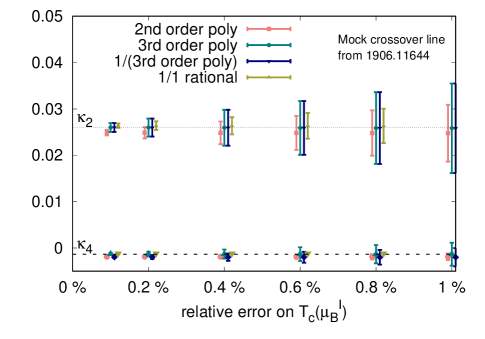
In the main text we calculated the transition temperature with sub-percent precision. This precision is needed when we are attempting to calculate a numerical derivative of with respect to the chemical potential. The relevance of the sub-percent errors in the determination can be highlighted in a mock analysis that we present below.
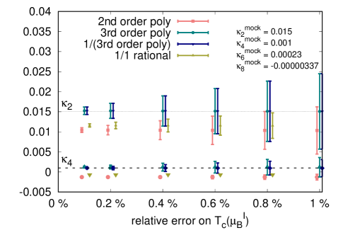
We took two model scenarios for the crossover line and generated mock data at imaginary chemical potential. Each mock data set was generated from a fourth order polynomial in with coefficients . For the first model, we fitted the cross-over line at real from Ref. Isserstedt et al. (2019), and obtained the following values for the coefficients: , , and . We then generated seven sets of mock data for each value of imaginary chemical potential listed in Eq. (7), assigning to each set a fixed relative error, ranging from to (see the left panel of Fig. 6). We fitted each set of mock data with four fit functions: a 2nd order polynomial, a 1/1 rational function , a third order polynomial and its reciprocal. and were extracted as the leading Taylor coefficients of the fit functions. In the case of the two-parameter fits we dropped the largest imaginary chemical potential, so that all fits had four degrees of freedom.
We repeated the whole procedure with a second model, constructed with a parameter of opposite sign and same order of magnitude compared to the first one. For and we used plausible values from the literature: , , while we obtained and by forcing the cross-over line to take the temperature values MeV, MeV and MeV at , 0 and 3, respectively (see the right panel of Fig. 6).
The purpose of the analysis was to determine whether the fits can reproduce the and values from the mock data. We found that the two models behave quite differently, even for large errors. In the first one, all the fit functions reproduce the value of . In the second model, however, the second order fits yield , while its actual value is . The third order fits perform much better. For the second model, we find and from the per-mill precision mock data. However, with more precise data or a substantially higher value, the third order fits would fail as well. In order for to be negligible relative to in a fit where , the coefficients and must be separated by more than an order of magnitude.
Our real lattice data have a relative precision on near 2 per-mills. Thus, in our analysis it is essential to take at least third order polynomials to extract the cross-over line up to order .
Note also that, by reducing the relative error on from to , we significantly improved the 2nd order result on . However, when switching to 3rd order fit functions the error bars become as large as before. What was gained with the increased precision is an access to . This feature of deducing Taylor coefficients from polynomial fits is also pointed out in the main text.
.3 Error estimate
In most results of this work, the statistical errors dominate. They were calculated through the standard jackknife procedure with 48 bins. For each lattice size, temperature and chemical potential we produced several (uncorrelated) Monte Carlo streams. In most cases we calculated the chiral observables after every five double-length trajectories. The sequence of measurements in the Monte Carlo streams with equal bare parameters are concatenated (after skipping 1000 trajectories for thermalization). The 48 bins are formed by splitting up this sequence evenly.
Systematic errors are introduced every time we make an ambiguous choice in the analysis. Such choices include the scale setting variable, which can be either or , the interpolating function we fit on the zero temperature data and the one we use to fit the renormalized quantities. At several points in the analysis we must make various decisions – e.g. how many data points to include into a fit or what the specific interpolating function should be. Each time we pursue two or more choices, this results in splitting the analysis. The final result is then calculated in many slightly different versions. The width of their distribution yields the systematic error.
In this paper we give combined errors. For this purpose, we consider the cumulative distribution function (CDF) for observable
| (8) |
where we built a weighted sum of a Gaussian CDF corresponding to analysis with mean and variance and . We use uniform weights with the aforementioned cut in the fit quality . The upper (lower) edge of the error bar is defined as the value of the observable corresponding to the 84% (16%) level of the cumulative distribution function.
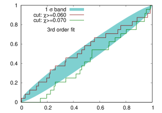
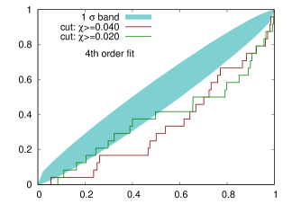
The different sources of systematic error in steps i-iv) of the analysis as described in the main text can be summarized as:
-
i)
2 choices of scale setting, 2 choices of the fit used for the renormalization of and 2 choices of the fit used for the renormalization of as discussed in the first supplement .1
-
ii)
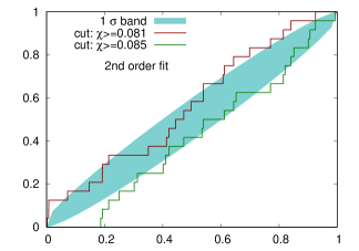
The function is fitted with a quadratic or cubic polynomial on the range given by . We choose two values for each polynomial order: we picked the largest and smallest values that are endorsed by a Kolmogorov-Smirnov test (see Fig. 7).
-
iii)
Two different cubic spline interpolations of . The spline node points are selected to be at every other simulation temperature (the separation of our simulation temperatures is 5 MeV or less, see Fig. 1 (left) in the main text). Here we use either every even or every odd simulation point as node points.
-
iv)
The global fit ansatz is either or with with , for the first fit and , for the second. As a further source of systematic error, we either include the largest imaginary chemical potential in this fit, or we drop it.
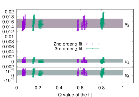
All these choices lead to the analyses mentioned in the main text. The values and the obtained and values for each fit are shown in Fig. 8. The fits are well spread in the interval, and there is no systematic dependence of the coefficients on the order of the used polynomial. There are no too bad or too good fits, either, these were sorted out by the Kolmogorov-Smirnoff tests of Fig. 7. This motivates us to combine the various analyses with a uniform weight. The error is mainly statistical. Among the statistical effects the precision of the peak position in is the bottleneck in this computation.
Notice our result on the coefficient in the bottom of Fig. 8. We cannot control the systematics of , nevertheless, we find it takes a small value, consistent with zero, and is stable for systematic effects. The order of magnitude of means that its effect on is not significant below .
.4 Strangeness neutrality
Throughout this work we use a strangeness chemical potential , which is always tuned such that for each simulated pair we have strangeness density . This is the strangeness neutrality condition. We have already calculated the dependence in Ref. Bellwied et al. (2015b), where we presented our first continuum extrapolated result on the curvature of the transition line.
As an improvement on our analysis from Ref. Bellwied et al. (2015b), we correct the renormalized chiral condensate and susceptibility for the systematic or statistical deviations from the strangeness neutrality condition. To this end, we calculate the derivatives of the condensate and the susceptibility with respect to the strangeness chemical potential.
Let us first write the observables for flavors at fixed chemical potential:
| (9) | |||||
| (10) | |||||
| (11) |
where:
| (12) | |||||
| (13) | |||||
| (14) |
Here stands for the Hermitian matrix where is the light quark matrix containing the light quark mass and the light quark chemical potential . At the same time we introduce the strange quark matrix containing the strange quark mass and the strange quark chemical potential . The lattice observable is the strange quark density, is the number of light flavors. The factor 1/4 in front of the trace in Eq. (14) is due to the use of staggered quarks.
We then calculate:
| (15) | |||||
| (16) | |||||
| (17) |
with
| (18) |
We can correct for the small deviations from that we find after performing the simulations, by calculating the change which would restore strangeness neutrality to leading order in a Taylor expansion on a jackknife-by-jackknife basis. We get the Taylor coefficients by averaging Eqs. (14) and (18) ensemble-by-ensemble:
| (19) |
We calculate the correction to the condensate and susceptibility to leading order in
| (20) | |||
| (21) |
where and are the renormalized observables from Eq. (2) of the main text. Thus, for our corrected ensembles strangeness neutrality is achieved with zero statistical error. The setup may have a systematic error, though, if the leading order expansion in was not satisfactory. However, the ensembles were already tuned to fulfill even without correction. The correction introduced here resulted in a relative shift of or less for both and .
The correction that we calculated in this elaborate analysis is found to be smaller than our statistical error in all cases, often by an order of magnitude. Nevertheless, we applied the correction for all lattice spacings that we use in this paper.
.5 Discussion of the width parameter
A natural definition of the width of the transition is given by the curvature at the peak of the susceptibility, i.e.
| (22) |
The second derivative of is numerically difficult to obtain, because it suffers from the systematic errors in the fit of . However, we can more easily model in a larger range of . Thus, we introduce a proxy for the half width
| (23) | |||||
where stands for the inverse function of . If we define analogously to Eq. (22) as
| (24) |
then using the fact that has a maximum at , i.e.
| (25) |
we find that up to higher order corrections in .
The values for this proxy are shown in Table 2. The proxy used in the main text – given by Eq. (4) – is even simpler. There, we fixed to its value for all chemical potentials. This is justified by the last column of Table 2: the value is consistent with all the values in the range. For this reason, at we have
| (26) |
| [MeV] | [MeV] | ||||
|---|---|---|---|---|---|
| 0.000 | 158.01(61) | 14.9(0.9) | 0.129(2) | 0.284(3) | 0.139(7) |
| 0.785 | 159.53(58) | 14.4(1.0) | 0.125(3) | 0.290(6) | 0.138(7) |
| 1.178 | 161.14(57) | 15.0(0.9) | 0.129(3) | 0.282(5) | 0.148(7) |
| 1.571 | 163.57(34) | 13.5(0.6) | 0.130(3) | 0.283(5) | 0.136(9) |
| 1.963 | 166.67(78) | 14.9(1.0) | 0.129(3) | 0.287(7) | 0.148(8) |
| 2.356 | 171.64(88) | 16.2(1.3) | 0.124(3) | 0.289(8) | 0.155(12) |
| 2.553 | 174.72(83) | 14.7(1.4) | 0.131(4) | 0.296(6) | 0.132(12) |
| 2.749 | 177.84(84) | 12.5(1.4) | 0.132(4) | 0.295(8) | 0.132(10) |
.6 Tabulated continuum extrapolated results
The extrapolation of presented in this letter is the result of a global correlated fit. We could have pursued a different strategy: calculate the continuum extrapolated curves for each imaginary , determine for each lattice at the given and then continuum extrapolate for fixed . This method has the advantage to yield statistically uncorrelated values. Its disadvantage is the lower precision: the simple polynomial continuum extrapolation of the entire function has a better fit quality if we restrict the data to a narrow peak region. Thus the best fits have fewer data points. Nevertheless, we tabulate statistically independent transition temperatures in Table 2, where the systematic errors are already included. In this table we give the other intermediate results as well: the width of the transition , the peak height , the renormalized chiral condensate and the width parameter .
In Table 3 we provide the extrapolated cross-over temperature and the width parameter at real from analytical continuation. They correspond to the green band in Fig. 3 and the blue band in the upper panel of Fig. 5, respectively. Unlike in Table 2, the errors here are correlated, since these results are the output of a global analysis.
| [MeV] | [MeV] | error [MeV] | [MeV] | error [MeV] |
|---|---|---|---|---|
| 000 | 158.08 | 0.47 | 14.47 | 0.31 |
| 020 | 158.03 | 0.48 | 14.46 | 0.32 |
| 040 | 157.92 | 0.48 | 14.45 | 0.33 |
| 060 | 157.72 | 0.48 | 14.43 | 0.36 |
| 080 | 157.45 | 0.49 | 14.41 | 0.42 |
| 100 | 157.08 | 0.51 | 14.36 | 0.50 |
| 120 | 156.63 | 0.54 | 14.31 | 0.62 |
| 140 | 156.08 | 0.60 | 14.23 | 0.79 |
| 160 | 155.43 | 0.69 | 14.14 | 1.03 |
| 180 | 154.67 | 0.83 | 14.01 | 1.36 |
| 200 | 153.77 | 1.04 | 13.84 | 1.80 |
| 220 | 152.72 | 1.35 | 13.61 | 2.41 |
| 240 | 151.50 | 1.78 | 13.30 | 3.23 |
| 260 | 150.04 | 2.39 | 12.89 | 4.35 |
| 280 | 148.29 | 3.28 | 12.32 | 5.92 |
| 300 | 146.16 | 4.62 | 11.49 | 8.22 |
References
- Aoki et al. (2006a) Y. Aoki, G. Endrodi, Z. Fodor, S. Katz, and K. Szabo, Nature 443, 675 (2006a), arXiv:hep-lat/0611014 [hep-lat] .
- Bhattacharya et al. (2014) T. Bhattacharya, M. I. Buchoff, N. H. Christ, H. T. Ding, R. Gupta, et al., (2014), arXiv:1402.5175 [hep-lat] .
- Aoki et al. (2006b) Y. Aoki, Z. Fodor, S. Katz, and K. Szabo, Phys.Lett. B643, 46 (2006b), arXiv:hep-lat/0609068 [hep-lat] .
- Aoki et al. (2009) Y. Aoki, S. Borsanyi, S. Durr, Z. Fodor, S. D. Katz, et al., JHEP 0906, 088 (2009), arXiv:0903.4155 [hep-lat] .
- Borsanyi et al. (2010) S. Borsanyi et al. (Wuppertal-Budapest Collaboration), JHEP 1009, 073 (2010), arXiv:1005.3508 [hep-lat] .
- Bazavov et al. (2012) A. Bazavov, T. Bhattacharya, M. Cheng, C. DeTar, H. Ding, et al., Phys.Rev. D85, 054503 (2012), arXiv:1111.1710 [hep-lat] .
- Allton et al. (2002) C. Allton, S. Ejiri, S. Hands, O. Kaczmarek, F. Karsch, et al., Phys.Rev. D66, 074507 (2002), arXiv:hep-lat/0204010 [hep-lat] .
- Allton et al. (2005) C. Allton, M. Doring, S. Ejiri, S. Hands, O. Kaczmarek, et al., Phys.Rev. D71, 054508 (2005), arXiv:hep-lat/0501030 [hep-lat] .
- Gavai and Gupta (2008) R. V. Gavai and S. Gupta, Phys. Rev. D78, 114503 (2008), arXiv:0806.2233 [hep-lat] .
- Basak et al. (2008) S. Basak et al. (MILC), Proceedings, 26th International Symposium on Lattice field theory (Lattice 2008), PoS LATTICE2008, 171 (2008), arXiv:0910.0276 [hep-lat] .
- Borsanyi et al. (2012a) S. Borsanyi, Z. Fodor, S. D. Katz, S. Krieg, C. Ratti, et al., JHEP 1201, 138 (2012a), arXiv:1112.4416 [hep-lat] .
- Borsanyi et al. (2012b) S. Borsanyi, G. Endrodi, Z. Fodor, S. Katz, S. Krieg, et al., JHEP 1208, 053 (2012b), arXiv:1204.6710 [hep-lat] .
- Bellwied et al. (2015a) R. Bellwied, S. Borsanyi, Z. Fodor, S. D. Katz, A. Pasztor, C. Ratti, and K. K. Szabo, Phys. Rev. D92, 114505 (2015a), arXiv:1507.04627 [hep-lat] .
- Ding et al. (2015) H. T. Ding, S. Mukherjee, H. Ohno, P. Petreczky, and H. P. Schadler, Phys. Rev. D92, 074043 (2015), arXiv:1507.06637 [hep-lat] .
- Bazavov et al. (2017) A. Bazavov et al., Phys. Rev. D95, 054504 (2017), arXiv:1701.04325 [hep-lat] .
- Bazavov et al. (2018) A. Bazavov et al., (2018), arXiv:1812.08235 [hep-lat] .
- Bazavov et al. (2020) A. Bazavov et al., (2020), arXiv:2001.08530 [hep-lat] .
- de Forcrand and Philipsen (2002) P. de Forcrand and O. Philipsen, Nucl. Phys. B642, 290 (2002), arXiv:hep-lat/0205016 [hep-lat] .
- D’Elia and Lombardo (2003) M. D’Elia and M.-P. Lombardo, Phys. Rev. D67, 014505 (2003), arXiv:hep-lat/0209146 [hep-lat] .
- D’Elia and Sanfilippo (2009) M. D’Elia and F. Sanfilippo, Phys. Rev. D80, 014502 (2009), arXiv:0904.1400 [hep-lat] .
- Cea et al. (2014) P. Cea, L. Cosmai, and A. Papa, Phys. Rev. D89, 074512 (2014), arXiv:1403.0821 [hep-lat] .
- Bonati et al. (2014) C. Bonati, P. de Forcrand, M. D’Elia, O. Philipsen, and F. Sanfilippo, (2014), arXiv:1408.5086 [hep-lat] .
- Cea et al. (2016) P. Cea, L. Cosmai, and A. Papa, Phys. Rev. D93, 014507 (2016), arXiv:1508.07599 [hep-lat] .
- Bonati et al. (2015) C. Bonati, M. D’Elia, M. Mariti, M. Mesiti, F. Negro, and F. Sanfilippo, Phys. Rev. D92, 054503 (2015), arXiv:1507.03571 [hep-lat] .
- Bellwied et al. (2015b) R. Bellwied, S. Borsanyi, Z. Fodor, J. Günther, S. D. Katz, C. Ratti, and K. K. Szabo, Phys. Lett. B751, 559 (2015b), arXiv:1507.07510 [hep-lat] .
- D’Elia et al. (2017) M. D’Elia, G. Gagliardi, and F. Sanfilippo, Phys. Rev. D95, 094503 (2017), arXiv:1611.08285 [hep-lat] .
- Gunther et al. (2017) J. Gunther, R. Bellwied, S. Borsanyi, Z. Fodor, S. D. Katz, A. Pasztor, and C. Ratti, Proceedings, 12th Conference on Quark Confinement and the Hadron Spectrum (Confinement XII): Thessaloniki, Greece, EPJ Web Conf. 137, 07008 (2017), arXiv:1607.02493 [hep-lat] .
- Alba et al. (2017) P. Alba et al., Phys. Rev. D96, 034517 (2017), arXiv:1702.01113 [hep-lat] .
- Vovchenko et al. (2017) V. Vovchenko, A. Pasztor, Z. Fodor, S. D. Katz, and H. Stoecker, Phys. Lett. B775, 71 (2017), arXiv:1708.02852 [hep-ph] .
- Bonati et al. (2018) C. Bonati, M. D’Elia, F. Negro, F. Sanfilippo, and K. Zambello, Phys. Rev. D98, 054510 (2018), arXiv:1805.02960 [hep-lat] .
- Borsanyi et al. (2018) S. Borsanyi, Z. Fodor, J. N. Guenther, S. K. Katz, K. K. Szabo, A. Pasztor, I. Portillo, and C. Ratti, JHEP 10, 205 (2018), arXiv:1805.04445 [hep-lat] .
- Fodor and Katz (2002) Z. Fodor and S. Katz, JHEP 0203, 014 (2002), arXiv:hep-lat/0106002 [hep-lat] .
- Fodor and Katz (2004) Z. Fodor and S. Katz, JHEP 0404, 050 (2004), arXiv:hep-lat/0402006 [hep-lat] .
- Fodor et al. (2019) Z. Fodor, M. Giordano, J. N. Günther, K. Kapás, S. D. Katz, A. Pásztor, I. Portillo, C. Ratti, D. Sexty, and K. K. Szabó, Proceedings, 27th International Conference on Ultrarelativistic Nucleus-Nucleus Collisions (Quark Matter 2018): Venice, Italy, May 14-19, 2018, Nucl. Phys. A982, 843 (2019).
- Giordano and Psztor (2019) M. Giordano and A. Psztor, Phys. Rev. D99, 114510 (2019), arXiv:1904.01974 [hep-lat] .
- Mukherjee and Skokov (2019) S. Mukherjee and V. Skokov, (2019), arXiv:1909.04639 [hep-ph] .
- Giordano et al. (2019) M. Giordano, K. Kapas, S. D. Katz, D. Nogradi, and A. Pasztor, (2019), arXiv:1911.00043 [hep-lat] .
- Kaczmarek et al. (2011) O. Kaczmarek, F. Karsch, E. Laermann, C. Miao, S. Mukherjee, et al., Phys.Rev. D83, 014504 (2011), arXiv:1011.3130 [hep-lat] .
- Endrodi et al. (2011) G. Endrodi, Z. Fodor, S. Katz, and K. Szabo, JHEP 1104, 001 (2011), arXiv:1102.1356 [hep-lat] .
- Isserstedt et al. (2019) P. Isserstedt, M. Buballa, C. S. Fischer, and P. J. Gunkel, Phys. Rev. D100, 074011 (2019), arXiv:1906.11644 [hep-ph] .
- Andronic et al. (2006) A. Andronic, P. Braun-Munzinger, and J. Stachel, Nucl.Phys. A772, 167 (2006), arXiv:nucl-th/0511071 [nucl-th] .
- Becattini et al. (2013) F. Becattini, M. Bleicher, T. Kollegger, T. Schuster, J. Steinheimer, et al., Phys.Rev.Lett. 111, 082302 (2013), arXiv:1212.2431 [nucl-th] .
- Alba et al. (2014) P. Alba, W. Alberico, R. Bellwied, M. Bluhm, V. Mantovani Sarti, et al., Phys.Lett. B738, 305 (2014), arXiv:1403.4903 [hep-ph] .
- Vovchenko et al. (2016) V. Vovchenko, V. V. Begun, and M. I. Gorenstein, Phys. Rev. C93, 064906 (2016), arXiv:1512.08025 [nucl-th] .
- Adamczyk et al. (2017) L. Adamczyk et al. (STAR), Phys. Rev. C96, 044904 (2017), arXiv:1701.07065 [nucl-ex] .
- Tanabashi et al. (2018) M. Tanabashi et al. (Particle Data Group), Phys. Rev. D98, 030001 (2018).
- Borsanyi et al. (2012c) S. Borsanyi, S. Durr, Z. Fodor, C. Hoelbling, S. D. Katz, et al., JHEP 1209, 010 (2012c), arXiv:1203.4469 [hep-lat] .
- Borsanyi et al. (2016) S. Borsanyi et al., Nature 539, 69 (2016), arXiv:1606.07494 [hep-lat] .
- Bellwied et al. (2019) R. Bellwied, S. Borsanyi, Z. Fodor, J. N. Guenther, J. Noronha-Hostler, P. Parotto, A. Pasztor, C. Ratti, and J. M. Stafford, (2019), arXiv:1910.14592 [hep-lat] .