Measurability of Coulomb wavepacket scattering effects

Abstract

A previous paper [J. Phys. B: At. Mol. Opt. Phys. 50, 215302 (2017)] showed that partial wave analysis becomes applicable to nonrelativistic Coulomb scattering if wavepackets are used. The scattering geometry considered was special: that of a head-on collision between the wavepacket and the centre of the potential. Our results predicted, in this case, a shadow zone of low probability for small angles around the forward direction for the description of alpha scattering from a gold foil. In this paper we generalize the results to the case of a nonzero impact parameter, a displacement of the wavepacket centre perpendicular to the average momentum direction. We predict a large flux in the forward direction from events with large impact parameters. We find a significant probability of scattering into the deviation region for impact parameters of order the spatial width of the wavepacket. Averaging over impact parameters produces predictions in excellent agreement with the Rutherford formula down to lower angles than for the zero impact parameter prediction. We consider issues that would arise in a real experiment and discuss the possibility of measuring a deviation from the Rutherford formula.

I Introduction

In a previous paper Hoffmann2017a , this author developed the scattering theory for a wavepacket in a Coulomb potential. The method used was partial wave analysis, which had been thought to be inapplicable to the Coulomb potential because the sum over the angular momentum index, $l,$ diverges for a plane wave treatment. The use of wavepackets was found to introduce a convergence factor into that sum. Then we summed the series numerically for a variety of cases, using the phase shifts obtained from the exact solution for the partial wave energy eigenvectors Messiah1961 .

We found generally excellent agreement with the Rutherford scattering cross section,

$$\frac{d\sigma}{d\Omega}_{\mathrm{Rutherford}}=\frac{Z_{1}^{2}Z_{2}^{2}\alpha^{2}}{16E^{2}\sin^{4}(\frac{\theta}{2})},$$ (1)

but found deviations in all cases, at low scattering angles. Here $Z_{1}$ and $Z_{2}$ are the atomic numbers of the target and projectile, respectively, $\alpha$ is the fine structure constant, $E$ is the incident energy and $\theta$ is the scattering angle.

Our method calculates probabilities of wavepacket-to-wavepacket transitions. We derived a formula that relates these probabilities to the differential cross section (see Eq. (25)). Since a probability is constrained to be less than unity while the Rutherford formula diverges in the forward direction, a disagreement was inevitable.

The aim of this paper is to investigate these disagreements with the Rutherford formula to see if any of them might be experimentally measurable.

For incident energies typical of scattering experiments that have been performed, we predict small probabilities of scattering into a small angular region around the forward direction, which we call a shadow zone. This is shown in Figure 1 for alpha particles of incident energy $E=4.8\,\mathrm{MeV}$ on gold foil with a momentum resolution parameter $\epsilon=0.001$ (see Eq. (6)).

Figure 1: Shadow zone for $E=4.8\,\mathrm{MeV},$ alpha on gold, $\epsilon=0.001.$ Probability (solid) compared to the Rutherford probability (dotted). The vertical, dashed, line shows our estimate, $\theta_{D}=4\epsilon|\eta|,$ for the size of the region of deviation from the Rutherford formula. This is for a head-on collision (zero impact parameter).

This prediction is in disagreement with the experimental observation of a high particle flux peaked around the forward direction. In this paper, we argue that the reason for this disagreement is the special scattering geometry that was chosen for the previous calculations. We modelled only a head-on collision, with the centre of the wavepacket approaching the centre of the potential. In this paper we investigate the effects of nonzero impact parameters, displacements perpendicular to the average direction of motion. Our physical expectation is that for an event with a sufficiently large impact parameter, the wavepacket will pass the potential largely undisturbed to contribute to a strong peak around the forward direction. The shadow zone around the forward direction for zero impact parameter is then seen as an interesting feature of the wave nature of the scattering, but may not be experimentally observable.

To proceed with these investigations, in Section II, we construct the wavefunctions and then the scattering probability for nonzero impact parameters. In Section III, we use this probability to confirm the result just postulated, that at sufficiently high impact parameter, the wavepacket emerges largely undisturbed, with nearly unit probability, moving in the forward direction.

In Section IV, we consider a model Coulomb scattering experiment, very similar to the original experiments of Geiger, Marsden and Rutherford Geiger1909 ; Rutherford1911 . It is only necessary to have better collimation of the beam of alpha particles to resolve details at low angles. To model an experiment, it is necessary to integrate probabilities over impact parameters. This is done for three angles in the deviation region and the results compared to the Rutherford prediction.

Conclusions follow in Section V.

II Scattering probability and cross section for nonzero impact parameter

The geometry we consider, modified from Hoffmann2017a to include nonzero impact parameters, is shown in Figure 2.

Figure 2: Scattering geometry with nonzero impact parameters.

Our method involves first transforming the free wavefunction of the incident projectile from a basis of eigenvectors of momentum, $\boldsymbol{k},$ to a basis of eigenvector of momentum magnitude, $k,$ and angular momentum, with indices $l,m.$ The transformation formula found in the earlier paper Hoffmann2017a is

$$\Psi_{\mathrm{free}}(k,l,m)=k\int_{0}^{\pi}\sin\theta_{k}d\theta_{k}\int_{0}^{2\pi}d\varphi_{k}\,Y_{lm}^{*}(\theta_{k},\varphi_{k})\psi_{\mathrm{free}}(\boldsymbol{k}).$$ (2)

The spherical harmonic can be written in terms of a Wigner rotation matrix

$$Y_{lm}^{*}(\theta_{k},\varphi_{k})=\sqrt{\frac{2l+1}{4\pi}}e^{-im\varphi}d_{m0}^{l}(\theta).$$ (3)

Choosing propagation in the $z$ direction with an impact parameter $\boldsymbol{b}=b\,\hat{\boldsymbol{x}}$ perpendicular to $\hat{\boldsymbol{z}}$ gives the simplest results. The $\boldsymbol{k}$ wavefunction for this geometry is chosen as

$$\psi_{\mathrm{free}}(\boldsymbol{k})=e^{-i\boldsymbol{k}\cdot\boldsymbol{b}}e^{-i\boldsymbol{k}\cdot\boldsymbol{R}_{i}}\frac{e^{-|\boldsymbol{k}-\boldsymbol{p}_{i}|^{2}/4\sigma_{p}^{2}}}{(2\pi\sigma_{p}^{2})^{\frac{3}{4}}}$$ (4)

with

$$\boldsymbol{p}_{i}=p\,\hat{\boldsymbol{z}},\quad\boldsymbol{R}_{i}=-R\,\hat{\boldsymbol{z}}.$$ (5)

The standard deviation of momentum is $\sigma_{p}$ in all directions. We choose the momentum resolution parameter

$$\epsilon=\frac{\sigma_{p}}{p}$$ (6)

to be much less than unity. The corresponding position wavefunction at $t=0$ has width $\sigma_{x}$ in all directions, with $\sigma_{x}\sigma_{p}=1/2.$ With the particular choice

$$R=\frac{1}{\sqrt{\epsilon}}\,\sigma_{x},$$ (7)

we ensure that the initial wavepacket is far from the origin (compared to the width), growing farther as $\epsilon$ is made smaller, but wavepacket spreading remains negligible over the course of the scattering experiment. Then $\sqrt{\epsilon}$ becomes the small parameter for our approximations.

In order to apply approximations, we impose a limit on the impact parameter

$$b\leq\frac{1}{\sqrt{\epsilon}}\,\sigma_{x}.$$ (8)

Then we expand

$$\boldsymbol{k}\cdot\boldsymbol{b}=bp\,\theta_{k}\cos\varphi_{k}+\mathcal{O}(\sqrt{\epsilon}).$$ (9)

Then the integral over $\varphi_{k}$ evaluates to (Gradsteyn1980 , their Eq. (8.411.1))

$$\int_{0}^{2\pi}d\varphi_{k}\,e^{-im\varphi_{k}}e^{-ibp\,\theta_{k}\cos\varphi_{k}}=2\pi\,e^{-i|m|\pi/2}J_{|m|}(bp\,\theta_{k}).$$ (10)

Next we use the low-angle approximation of the Wigner rotation matrix, uniform in $l,m,$ derived in Hoffmann2018b ,

$$d_{m0}^{l}(\theta_{k})\sim\Phi(m)\,[\frac{(l+|m|)!}{(l-|m|)!}]^{\frac{1}{2}}\frac{1}{\Lambda^{|m|}}J_{|m|}(\Lambda\theta_{k}),$$ (11)

with

$$\Lambda(l,m)=\sqrt{(l+\frac{1}{2})^{2}-\frac{1}{3}m^{2}+\frac{1}{12}}$$ (12)

and

$$\Phi(m)=\begin{cases}(-)^{m}&m\geq 0,\\ 1&m<0.\end{cases}$$ (13)

For $m=0$ and $l=2000,$ the absolute error in this approximation is less than $5\times 10^{-10}$ on $0\leq\theta\leq 0.2.$

We use the integral (Gradsteyn1980 , their Eq. (6.633.2))

$$\int_{0}^{\pi}\theta_{k}\,d\theta_{k}\,e^{-p^{2}\theta_{k}^{2}/4\sigma_{p}^{2}}\,J_{|m|}(\Lambda\theta_{k})J_{|m|}(bp\,\theta_{k})=2\epsilon^{2}e^{-\epsilon^{2}(\Lambda-bp)^{2}}e^{-2\epsilon^{2}\Lambda bp}I_{|m|}(2\epsilon^{2}\Lambda bp).$$ (14)

Noting

$$\Phi(m)\,e^{-i|m|\pi/2}=e^{im\pi/2},$$ (15)

we find the free wavefunction in the $k,l,m$ basis

$$\Psi_{\mathrm{free}}(k,l,m)=e^{im\pi/2}e^{+ikR}\frac{e^{-(k-p)^{2}/4\sigma_{p}^{2}}}{(2\pi\sigma_{p}^{2})^{\frac{1}{4}}}2\epsilon\sqrt{l+\frac{1}{2}}[\frac{(l+|m|)!}{(l-|m|)!}]^{\frac{1}{2}}\frac{1}{\Lambda^{|m|}}e^{-\epsilon^{2}(\Lambda-bp)^{2}}\mu_{|m|}(2\epsilon^{2}\Lambda bp),$$ (16)

with

$$\mu_{|m|}(z)\equiv e^{-z}\,I_{|m|}(z).$$ (17)

The following steps are very similar to those in Hoffmann2017a , so will not be repeated here. Only phase shifts can be applied to the free $k,l,m$ wavefunction to produce the incoming $k,l,m$ wavefunction, to preserve

$$|\Psi_{\mathrm{in}}(k,l,m)|^{2}\rightarrow|\Psi_{\mathrm{free}}(k,l,m)|^{2}\quad\mathrm{as}\ \epsilon\rightarrow 0^{+}.$$ (18)

Those phase shifts are found in terms of the Coulomb phase shifts Messiah1961

$$e^{i2\sigma_{l}(k)}=\frac{\Gamma(l+1+i\eta(k))}{\Gamma(l+1-i\eta(k))}$$ (19)

(with $\eta(k)=\alpha/(k/m_{0})$ a dimensionless measure of the strength of the interaction) and the expansion of the logarithmic term, $\eta(k)\ln(2kr),$ that appears in the asymptotic approximation of the Coulomb spherical waves. Applying this phase shift ensures that the position probability density of the interacting state vector satisfies

$$|\psi_{\mathrm{in}}(\boldsymbol{r})|^{2}\rightarrow|\psi_{\mathrm{free}}(\boldsymbol{r})|^{2}\quad\mathrm{as}\ \epsilon\rightarrow 0^{+}.$$ (20)

The outgoing state vector is constructed from the incoming by applying the antiunitary time reversal operator (which complex conjugates the phase shifts) and a rotation into the final scattering angle, $\theta.$ Note that by conservation of angular momentum, the final state will have the same average impact parameter as the initial state.

We find the result for the probability of a wavepacket to wavepacket transition

$$P(\theta,\eta,\beta,\delta,\epsilon)=\left|\sum_{l=0}^{\infty}\sum_{m_{f}=-l}^{l}\sum_{m_{i}=-l}^{l}\Phi_{\mathrm{free}}(l,m_{f})e^{+i(m_{i}-m_{f})\pi/2}d_{m_{i}m_{f}}^{(l)}(\theta)\Phi_{\mathrm{free}}(l,m_{i})e^{i2\sigma_{l}(p)}e^{-(\delta-\xi_{l})^{2}/8}\right|^{2},$$ (21)

where

$$\xi_{l}\equiv 4\epsilon\eta(p)\{\ln(2pR)-1-\frac{\partial\sigma_{l}[\eta(p)]}{\partial\eta}\}$$ (22)

and

$$\Phi_{\mathrm{free}}(l,m) =2\epsilon\sqrt{l+\frac{1}{2}}\,[\frac{(l+|m|)!}{(l-|m|)!}]^{\frac{1}{2}}\frac{1}{\Lambda^{|m|}}e^{-\epsilon^{2}(\Lambda-bp)^{2}}\mu_{|m|}(2\epsilon^{2}\Lambda bp)$$ (23)

and $\beta=b/\sigma_{x}$ is a dimensionless measure of the impact parameter. Here

$$\delta(T)=\frac{\frac{p}{m_{0}}T-2R}{\sigma_{x}}$$ (24)

in terms of the interaction time, $T,$ and the mass, $m_{0},$ of the projectile. Plotting the probability versus $\delta$ shows a peak shifted in time, with the position of the maximum, $\delta_{\mathrm{max}},$ showing a time delay if $\delta_{\mathrm{max}}>0$ and an advancement if $\delta_{\mathrm{max}}<0.$ In practice, we find the value, $\delta_{\mathrm{max}},$ that maximizes the probability, then recalculate the probability with $\delta$ set to that value.

According to a formula derived in Hoffmann2017a , the differential cross section is related to the probability by

$$\frac{d\sigma}{d\Omega}=\frac{p^{2}}{16\,\sigma_{p}^{4}}P(\theta,\eta,\beta,\delta,\epsilon),$$ (25)

valid for Gaussian wavepackets. We apply this to the Rutherford differential cross section to form a dimensionless “probability”, not a true probability since it rises greater than unity,

$$P_{\mathrm{Ruth}}(\theta,\eta,\epsilon)=\frac{4\epsilon^{4}\eta^{2}}{\sin^{4}\frac{\theta}{2}}.$$ (26)

III Scattering into the forward direction

We start by considering the question of the influence of nonzero impact parameters on the scattering into the forward direction.

We consider the original experiment performed by Geiger, Marsden and Rutherford Geiger1909 ; Rutherford1911 , with an alpha particle of energy $E=4.8\,\mathrm{MeV}$ from Radium-226 incident on a thin gold foil. This gives the strength parameter $\eta=22.8.$ (Note this was incorrectly stated as $\eta=23.1$ in Hoffmann2017a .) We choose the momentum resolution parameter $\epsilon=0.001$ which gives $\sqrt{\epsilon}=0.032.$ Note that energy linewidths as small as $\Delta E=2\,\mathrm{keV}$ have been observed Pomme2015 using extremely thin radium samples. This would imply that the momentum resolution parameter was $\epsilon\leq 2.1\times 10^{-4}$ for those sources.

The alpha particle wavepackets (of spatial width $\sigma_{x}=0.0052\,\textrm{\r{A}}$) will approach the gold nuclei with every impact parameter between 0 and approximately half the internuclear distance of $2.6\,\textrm{\r{A}}$ (corresponding to $\beta=250$ with the parameters we have chosen). Note that the optimal starting separation from the nucleus is only $R=0.16\,\textrm{\r{A}},$ indicating that it is very difficult, in practice, to create an ideal scattering experiment where wavepacket spreading is negligible.

For those events with small impact parameters, we expect that there will be scattering into all directions. In an event with sufficiently large impact parameter, it is our physical hypothesis that the wavepacket will pass the nucleus largely undisturbed and contribute to a peak of flux in the forward direction.

We confirm this expectation now by calculating the probabilities for a range of impact parameters of scattering into the forward direction. In that case

$$d_{m_{i}m_{f}}^{(l)}(0)=\delta_{m_{i}m_{f}}$$ (27)

and the scattering probability reduces to

$$P(0,\eta,\beta,\delta,\epsilon)=\left|\sum_{l=0}^{\infty}\sum_{m=-l}^{l}4\epsilon^{2}(l+\frac{1}{2})\frac{(l+|m|)!}{(l-|m|)!}\frac{1}{\Lambda^{2|m|}}e^{-2\epsilon^{2}(\Lambda-bp)^{2}}\mu_{|m|}^{2}(2\epsilon^{2}\Lambda bp)\,e^{i2\sigma_{l}(p)}e^{-(\delta-\xi_{l})^{2}/8}\right|^{2}.$$ (28)

We can simplify this expression if we only consider impact parameters $\beta\geq 10.$ Then the probability distribution in $l$ is centred on the magnitude of the classical angular momentum $L=bp,$ with a width of order $1/\epsilon=1000.$ So low values of $l$ are suppressed. The classical angular momentum vector has vanishing component in the $z$ direction, a consequence of our choice of scattering geometry. So the probability distribution in $m$ is centred on $m=0$ with a width that we estimate as $\Delta m\sim\beta/\sqrt{2}$ (see Eq. (39)). These features are shown in Figure 3, where we plot $|\Phi_{\mathrm{free}}(l,m)|^{2}.$

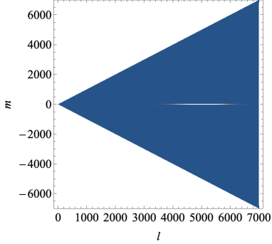
Figure 3: Probability density in $l$ and $m$ for $\beta=10$ (absolute values not determined).

Then we have

$$\frac{|m|}{l}\sim\frac{\epsilon}{2}\ll 1.$$ (29)

Then we can use the Stirling approximation (Gradsteyn1980 , their Eq. (8.327)) for the factorials

$$\frac{(l+|m|)!}{(l-|m|)!}=l^{2|m|}\{1+\mathcal{O}(\frac{|m|}{l})\}.$$ (30)

In this approximation $\Lambda$ can be replaced by $l,$ and

$$\Lambda^{2|m|}=l^{2|m|}\{1+\mathcal{O}(\frac{|m|}{l})\}.$$ (31)

In Appendix A we derive an asymptotic approximation for $\mu_{|m|}(z),$ for $z\gg 1,$ uniform in $m$

$$\mu_{|m|}(z)\sim\frac{e^{-(m^{2}-\frac{1}{4})/2z}}{\sqrt{2\pi z}}.$$ (32)

Here $z$ will be of order $z\sim\beta^{2}/2\geq 50.$

Then the simplified probability is

$$P(0,\eta,\beta,\delta,\epsilon) \sim\left|\sum_{l=0}^{\infty}4\epsilon^{2}(l+\frac{1}{2})e^{-2\epsilon^{2}(l-bp)^{2}}\sum_{m=-l}^{l}\frac{e^{-(m^{2}-\frac{1}{4})/2\epsilon^{2}lbp}}{4\pi\epsilon^{2}lbp}\,e^{i2\sigma_{l}(p)}e^{-(\delta-\xi_{l})^{2}/8}\right|^{2}$$

$$\sim\left|\sum_{l=0}^{\infty}4\epsilon^{2}(l+\frac{1}{2})\frac{e^{-2\epsilon^{2}(l-bp)^{2}}}{\sqrt{8\pi\epsilon^{2}lbp}}\,e^{i2\sigma_{l}(p)}e^{-(\delta-\xi_{l})^{2}/8}\right|^{2}.$$ (33)

We evaluated this expression numerically for $\eta=22.8,$ on $10\leq\beta\leq 250.$ No correction was made for time shifts, which were found to be small ($\delta$ was set to 0). The result is shown in Figure 4, and confirms our hypothesis.

Note that there is another matter to consider. This result is for alpha particles scattering off a single bare nucleus. In an experiment, the alphas at high impact parameter and low momentum transfer would be scattering off effectively neutral atoms, screened by the electrons. This would make the forward flux even larger than this prediction.

That the forward probability remains small for low impact parameters is an interesting prediction, but would not be measurable unless the impact parameter of a collision could be controlled to much less than an Angstrom.

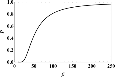
Figure 4: Probability of scattering into the forward direction as a function of impact parameter for $\eta=22.8.$

IV Deviations from the Rutherford formula at low scattering angles

In a Rutherford scattering experiment described in Melissinos2003 , the source was the $E=5.2\,\mathrm{MeV}$ emission from Polonium-210 ($\eta=21.9$). Those researchers were able to collimate their source so that the unscattered beam extended to approximately $4^{\circ}=0.070\,\mathrm{rad}.$ We suppose that this could be done with an $E=4.8\,\mathrm{MeV}$ source. From Figure 1, we see deviations from the Rutherford formula for the zero impact parameter prediction on $0\leq\theta\leq 0.2,$ for $\epsilon=0.001.$ Our estimate for the size of the deviation region is Hoffmann2017a

$$\theta_{D}=4\epsilon|\eta|,$$ (34)

proportional to $\epsilon.$ So deviations could possibly be observed for $\epsilon\geq 10^{-3}$ but not for $\epsilon=10^{-4}.$ Note that the smallest angle (other than the forward direction) at which measurements were taken in the aforementioned experiment was $6^{\circ}=0.10\,\mathrm{rad}.$

Making predictions just with the $\beta=0$ profile does not give an accurate portrayal of an experiment. Yet it gives good agreement with experiment on $\theta\geq 0.2.$ An integration is needed over the distribution of impact parameters, vectors in the $xy$ plane according to Figure 2. We label them with a radial coordinate, $\beta,$ and an azimuthal angle, $\varphi.$

We will implement this integration shortly, but first we need a result from it to justify a step in the procedure. At $\theta=\pi/2,$ far from the possible deviation region, we find, after correcting for a time shift,

$$P(\frac{\pi}{2},22.8,\beta,\varphi,0.6,0.001)\sim P_{\mathrm{Ruth}}(\frac{\pi}{2},22.8,0.001)\,e^{-b^{2}/\sigma_{x}^{2}},$$ (35)

independent of $\varphi.$ Then we have

$$\frac{\int d^{2}b\,P(\frac{\pi}{2},22.8,\beta,\varphi,0.6,0.001)}{\int d^{2}b\,e^{-b^{2}/\sigma_{x}^{2}}}=\frac{\int d^{2}b\,P_{\mathrm{Ruth}}(\frac{\pi}{2},22.8,0.001)\,e^{-b^{2}/\sigma_{x}^{2}}}{\pi\sigma_{x}^{2}}=P_{\mathrm{Ruth}}(\frac{\pi}{2},22.8,0.001).$$ (36)

With the area $A=\pi\sigma_{x}^{2}$ in the denominator, this averaging just returns the Rutherford prediction, as required. Then we take the same area at all angles (and any $\epsilon$) and replace

$$P(\theta,22.8,0,0,\delta,\epsilon)\rightarrow\frac{\int d^{2}b\,P(\theta,22.8,\beta,\varphi,\delta,\epsilon)}{\pi\sigma_{x}^{2}}=\frac{1}{\pi}\int_{0}^{\infty}\beta\,d\beta\int_{0}^{2\pi}d\varphi\,P(\theta,22.8,\beta,\varphi,\delta,\epsilon).$$ (37)

The initial and final state vectors are modified to

$$|\,\boldsymbol{p}_{i},-R\hat{\boldsymbol{z}}+\boldsymbol{b}(\varphi);\mathrm{in}\,\rangle =U(R_{z}(\varphi))\,|\,\boldsymbol{p}_{i},-R\hat{\boldsymbol{z}}+b\hat{\boldsymbol{x}};\mathrm{in}\,\rangle,$$

$$|\,\boldsymbol{p}_{f},R_{y}(\theta)\{+R\hat{\boldsymbol{z}}+\boldsymbol{b}(\varphi)\};\mathrm{out}\,\rangle =U(R_{y}(\theta+\pi))U(R_{z}(-\varphi))A(\mathcal{T})\,|\,\boldsymbol{p}_{i},-R\hat{\boldsymbol{z}}-b\hat{\boldsymbol{x}};\mathrm{in}\,\rangle.$$ (38)

This introduces a factor $\exp(-i(m_{i}-m_{f})\varphi)$ inside the sums in Eq. (21).

We will only consider scattering angles in $0.1\leq\theta\leq 0.2.$ Then we will find that it suffices to integrate up to a scaled impact parameter $\beta=3$ (see Figure 5 (a)). The width in $m$ of the function $\mu_{|m|}(2\epsilon^{2}\Lambda bp)$ is, from Eq. (32),

$$\Delta m=\sqrt{2\epsilon^{2}\Lambda bp}\sim\sqrt{2\epsilon^{2}(bp)^{2}}=\frac{1}{\sqrt{2}}\beta,$$ (39)

using $\Lambda\sim bp$ at the wavefunction peak. So we expect that it will be sufficient to consider $m_{f},m_{i}$ values in Eq. (21) in the range $|m_{f}|,|m_{i}|\leq 2.$

Again we are able to approximate

$$[\frac{(l+|m|)!}{(l-|m|)!}]^{\frac{1}{2}}\frac{1}{\Lambda^{|m|}}\sim 1$$ (40)

and replace $\Lambda$ with $l.$

Since we are only considering small angles, we can use the small angle approximation of the Wigner rotation matrices found in Hoffmann2018b . There are problems with evaluating Wigner rotation matrices of large order in MATHEMATICA Mathematica2019 . These problems are avoided with this approximation in terms of Bessel functions. We use

$$d_{m_{i}m_{f}}^{l}(\theta)\sim(-)^{m_{i}-m_{f}}(\frac{\theta}{\sin\theta})^{\frac{1}{2}}J_{m_{i}-m_{f}}(l\theta)\quad\mathrm{for}\ m_{i}\geq m_{f}$$ (41)

and

$$d_{m_{1}m_{2}}^{j}(\theta)=(-)^{m_{1}-m_{2}}d_{m_{2}m_{1}}^{j}(\theta).$$ (42)

Summing the relevant terms in Eq. (21) gives

$$P(\theta,\eta,\beta,\delta) \sim\frac{\theta}{\sin\theta}|\sum_{l=0}^{\infty}4\epsilon^{2}(l+\frac{1}{2})\,e^{-2\epsilon^{2}(l-bp)^{2}}e^{i2\sigma_{l}(p)}e^{-(\delta-\xi_{l})^{2}/8}\{J_{0}(\mu_{0}^{2}+2\mu_{1}^{2}+2\mu_{2}^{2})-iJ_{1}\mu_{2}\mu_{1}4\cos\varphi-iJ_{1}\mu_{1}\mu_{0}4\cos\varphi$$

$$\quad-J_{2}\mu_{2}\mu_{0}4\cos(2\varphi)-J_{2}\mu_{1}^{2}2\cos(2\varphi)+iJ_{3}\mu_{2}\mu_{1}4\cos(3\varphi)+J_{4}\mu_{2}^{2}2\cos(4\varphi)\}|^{2},$$ (43)

where

$$J_{n}=J_{n}(l\theta),\quad\mu_{n}=\mu_{n}(\epsilon l\beta),\quad n=0,1,2,\dots.$$ (44)

Using this, we found the probability at $\theta=\pi/2$ to be independent of $\varphi,$ as discussed above. At $\theta=0.1,$ for example, we find dependence on both $\beta$ and $\varphi,$ as seen in Figure 5.

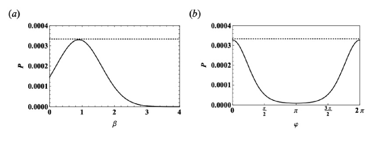
Figure 5: Dependence of probabilities on (a) $\beta$ and (b) $\varphi$ at $\theta=0.1.$

Evaluating Eq. (43) numerically for $\theta=0.10,0.15,0.20$ gives the results shown in Figure 6. The Rutherford probability and the zero impact parameter prediction are shown for comparison. Remarkably, the integration over impact parameters supplies the missing probability needed to give excellent agreement with the Rutherford formula.

We have not done an analysis of the propagation of errors from our approximation procedures. We note that the differences of our predictions from the Rutherford formula for $\theta=0.10,0.15,0.20$ are all less than $1\,\%.$

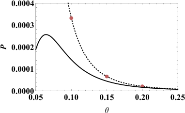
Figure 6: Results of integration over impact parameter, showing probabilities as points. The Rutherford probability (dotted) and the zero impact parameter prediction (solid) are shown for comparison

This process cannot continue to arbitrarily small scattering angles. The Rutherford “probability”, Eq. (26), reaches unity at

$$\theta_{1}=\epsilon\sqrt{8|\eta|}=0.014$$ (45)

with our parameters, so deviations are inevitable below that angle. For impact parameters with $\beta\geq 10,$ the character of the probability profile changes, as we will discuss in a future paper. The major contributions to probability then come at angles smaller than the minimum considered here, $\theta=0.1.$ Deviations from the Rutherford formula are then probable, after integration over impact parameters. Of course measurements at low angles would require an incoming beam collimated to a small angular width. This would decrease the count rate, but in this region the expected count rates are the highest.

A significant unknown in this analysis is the size of the wavepackets from a given source, or the distribution of sizes. If a source was producing wavepackets with $\epsilon\leq 2.1\times 10^{-4},$ as was discussed in Section III, there would be little chance of ever measuring deviations from the Rutherford formula. However it may be possible to increase the fractional momentum width, $\epsilon,$ from a source, say by increasing the thickness of the radioactive layer. The value $\epsilon=0.001$ considered here was chosen as low but not excessively low, with the error factor $\sqrt{\epsilon}$ acceptably low. Unfortunately, the current state of alpha particle spectrometers Ruddy2006 is not sufficient to resolve a linewidth with $\Delta E/E=2\epsilon=0.002.$

V Conclusions

The aim of this paper was to investigate whether the shadow zone of low scattering probability around the forward direction predicted for zero impact parameter would persist when nonzero impact parameters were considered. The first calculation we performed indicated that, for events with impact parameters much larger than the wavepacket width, the wavepackets would exit into the forward direction largely undisturbed by the interaction. This confirms an obvious feature of a Coulomb scattering experiment: the strong signal in the forward direction from the unscattered part of the beam.

Then we found that events with impact parameters of order the wavepacket width introduce significant probability into the region of deviation from the Rutherford formula (for $\beta=0$). For a beam with a distribution of impact parameters, averaging over impact parameters is necessary to construct a prediction. We did this for three low angles in the region of deviation and found, remarkably, predictions in excellent agreement with the Rutherford formula. This extends the validity of that formula further down into the deviation zone.

There may still be deviations from that formula that could be measured experimentally, with a well-collimated alpha beam (at the expense of lower count rates). Further investigation, focussing on even larger impact parameters, will be done in a future paper.

Appendix A Asymptotic approximation of $\mu_{|m|}(z)$

The defining differential equation for the modified Bessel functions, $I_{\nu}(z),$ is (DLMF2020 , their Eq. (10.25.1))

$$\{\frac{d^{2}}{dz^{2}}+\frac{1}{z}\frac{d}{dz}-(1+\frac{\nu^{2}}{z^{2}})\}I_{\nu}(z)=0.$$ (46)

The previously known asymptotic approximation for large $z$ is (DLMF2020 , their Eq. (10.40.1))

$$I_{\nu}(z)\sim\frac{e^{z}}{\sqrt{2\pi z}}\{1-\frac{\nu^{2}-1/4}{2z}+\mathcal{O}(\frac{1}{z^{2}})\}.$$ (47)

This does not capture the dependence on $\nu$ for large $\nu,$ so we seek an asymptotic approximation uniform in $\nu$ that holds for large $\nu.$

We write

$$I_{\nu}(z)=\frac{e^{x}}{\sqrt{2\pi x}}g_{\nu}(z).$$ (48)

Then we find the differential equation for $g_{\nu}(z)$ is

$$g_{\nu}^{\prime\prime}+2g_{\nu}^{\prime}-\frac{\nu^{2}-1/4}{z^{2}}g_{\nu}=0.$$ (49)

For large $z$ we scale this equation, writing

$$z=M\xi,$$ (50)

with $M\gg 1$ and $\xi$ of order unity. This gives

$$\frac{1}{M^{2}}\frac{d^{2}g_{\nu}}{d\xi^{2}}+\frac{2}{M}\frac{dg_{\nu}}{d\xi}-\frac{1}{M^{2}}\frac{\nu^{2}-1/4}{\xi^{2}}g_{\nu}=0.$$ (51)

Note that for $\nu$ of order $\sqrt{M},$ the third term becomes of the same order as the second.

Ignoring the first term gives

$$\frac{dg_{\nu}}{dz}\cong\frac{\nu^{2}-1/4}{2z^{2}}g_{\nu},$$ (52)

with solution

$$g_{\nu}(z)=C\,e^{-(\nu^{2}-\frac{1}{4})/2z}.$$ (53)

We set $C=1$ to find agreement with Eq. (47) for small $\nu.$ From our definition of $\mu_{|m|}(z),$ Eq. (32), we have the asymptotic approximation

$$\mu_{|m|}(z)\sim\frac{e^{-(m^{2}-\frac{1}{4})/2z}}{\sqrt{2\pi z}}.$$ (54)

We use this result to approximate the sum

$$S(z) =\sum_{m=-l}^{l}\mu_{|m|}^{2}(z)$$

$$\sim\sum_{m=-\infty}^{\infty}\frac{e^{-(m^{2}-\frac{1}{4})/z}}{2\pi z}$$

$$\sim\frac{1}{\sqrt{4\pi z}}.$$

A numerical check showed a fractional error in this approximation less than 0.0013 for $z\geq 50.$

References

- (1) Hoffmann SE. Prediction of deviations from the Rutherford formula for low-energy Coulomb scattering of wavepackets. Journal of Physics B: Atomic, Molecular and Optical Physics. 2017;50:215302.
- (2) Messiah A. Quantum Mechanics. vol. 1 and 2. North-Holland, Amsterdam and John Wiley and Sons, N.Y.; 1961.
- (3) Geiger H, Marsden E. On a diffuse reflection of the alpha particles. Proc Roy Soc. 1909;82:495.
- (4) Rutherford E. The scattering of and rays by matter and the structure of the atom. Phil Mag. 1911;Series 6, vol. 21:669.
- (5) Gradsteyn IS, Ryzhik IM. Tables of Integrals, Series and Products. Corrected and enlarged ed. Academic Press, Inc., San Diego, CA; 1980.
- (6) Hoffmann SE. Uniform analytic approximation of Wigner rotation matrices. J Math Phys. 2018;59:022102.
- (7) Pommé S. Typical uncertainties in alpha-particle spectrometry. Metrologia. 2015;52:S146.
- (8) Melissinos A, Napolitano J. Experiments in Modern Physics. Academic Press, Inc., San Diego, CA; 2003.
- (9) Mathematica; 2020. Wolfram Research Inc.
- (10) Ruddy FH, Seidel JG, Haoqian Chen, Dulloo AR, Sei-Hyung Ryu. High-resolution alpha-particle spectrometry using 4H silicon carbide semiconductor detectors. IEEE Trans Nucl Sci. 2006;53:1713.
- (11) NIST Digital Library of Mathematical Functions;. F. W. J. Olver et al., eds. http://dlmf.nist.gov/, Release 1.0.25 of 2019-12-15. Available from: http://dlmf.nist.gov/.