Perturbo: a software package for ab initio electron-phonon interactions,
charge transport and ultrafast dynamics

Abstract

Perturbo is a software package for first-principles calculations of charge transport and ultrafast carrier dynamics in materials. The current version focuses on electron-phonon interactions and can compute phonon-limited transport properties such as the conductivity, carrier mobility and Seebeck coefficient. It can also simulate the ultrafast nonequilibrium electron dynamics in the presence of electron-phonon scattering. Perturbo uses results from density functional theory and density functional perturbation theory calculations as input, and employs Wannier interpolation to reduce the computational cost. It supports norm-conserving and ultrasoft pseudopotentials, spin-orbit coupling, and polar electron-phonon corrections for bulk and 2D materials. Hybrid MPI plus OpenMP parallelization is implemented to enable efficient calculations on large systems (up to at least 50 atoms) using high-performance computing. Taken together, Perturbo provides efficient and broadly applicable ab initio tools to investigate electron-phonon interactions and carrier dynamics quantitatively in metals, semiconductors, insulators, and 2D materials.

PROGRAM SUMMARY

Program Title: Perturbo
Program summary URL: https://perturbo-code.github.io
Licensing provisions: GNU General Public Licence 3.0
Programming language: Fortran, Python
External routines/libraries: LAPACK, HDF5, MPI, OpenMP, FFTW, Quantum-ESPRESSO
Nature of problem: Computing transport properties from first-principles in materials, including the electrical conductivity, carrier mobility and Seebeck coefficient; Simulating ultrafast nonequilibrium electron dynamics, such as the relaxation of excited carriers via interactions with phonons.
Solution method: We implement the first-principles Boltzmann transport equation, which employs materials properties such as the electronic structure, lattice dynamics, and electron-phonon collision terms computed with density functional theory and density functional perturbation theory. The Boltzmann transport equation is solved numerically to compute charge transport and simulate ultrafast carrier dynamics. Wannier interpolation is employed to reduce the computational cost.
Additional comments: Hybrid MPI plus OpenMP parallelization is implemented to run large calculations and take advantage of high-performance computing. Most results are output to HDF5 file format, which is portable and convenient for post-processing using high-level languages such as Python and Julia.

1 Introduction

Understanding the dynamical processes involving electrons, lattice vibrations (phonons), atomic defects, and photons in the solid state is key to developing the next generation of materials and devices [1, 2]. Due to the increasing complexity of functional materials, there is a critical need for computational tools that can take into account the atomic and electronic structure of materials and make quantitative predictions on their physical properties. The vision behind Perturbo is to provide a unified platform and a validated code that can be applied broadly to compute the interactions, transport and ultrafast dynamics of electrons and excited states in materials [3]. The goal is to facilitate basic scientific discoveries in materials and devices by advancing microscopic understanding of carrier dynamics, while creating a sustainable software element able to address the demands of the computational physics community.
Perturbo builds on established first-principles methods. It uses density functional theory (DFT) and density functional perturbation theory (DFPT) [4] as a starting point for computing electron dynamics. It reads the output of DFT and DFPT calculations, for now from the Quantum Espresso (QE) code [5, 6], and uses this data to compute electron interactions, charge transport and ultrafast dynamics. The current distribution focuses on electron-phonon ($e$-ph) interactions and the related phonon-limited transport properties [7], including the electrical conductivity, mobility and the Seebeck coefficient. It can also simulate the ultrafast nonequilibrium electron dynamics in the presence of $e$-ph interactions. The developer branch, which is not publicly available yet, also includes routines for computing spin [8], electron-defect [9, 10], and electron-photon interactions [11], as well as advanced methods to compute the ultrafast dynamics of electrons and phonons in the presence of electric and magnetic fields. These additional features will be made available in future releases.
The transport module of Perturbo enables accurate calculations of charge transport in a wide range of functional materials. In its most basic workflow, Perturbo computes the conductivity and mobility as a function of temperature and carrier concentration, either within the relaxation time approximation (RTA) or with an iterative solution of the linearized Boltzmann transport equation (BTE) [12, 13]. The ultrafast dynamics module explicitly evolves in time the electron BTE (while keeping the phonon occupations fixed), enabling investigations of the ultrafast electron dynamics starting from a given initial electron distribution [14]. Our routines can carry out these calculations in metals, semiconductors, insulators, and 2D materials. An efficient implementation of long-range $e$-ph interactions is employed for polar bulk and 2D materials. Materials with spin-orbit coupling (SOC) are treated using fully relativistic pseudopotentials [8, 13]. Both norm-conserving and ultrasoft pseudopotentials are supported. Quantities related to $e$-ph interactions can be easily obtained, stored and analyzed.
Perturbo is implemented in modern Fortran with a modular code design. All calculations employ intuitive workflows. The code is highly efficient thanks to its hybrid MPI (Message Passing Interface) and OpenMP (Open Multi-Processing) parallelization. It can run on record-large unit cells with up to at least 50 atoms [15], and its performance scales up to thousands of CPU cores. It conveniently writes files using the HDF5 format, and is suitable for both high-performance supercomputers and smaller computer clusters.
Target users include both experts in first-principles calculations and materials theory as well as experimental researchers and teams in academic or national laboratories investigating charge transport, ultrafast spectroscopy, advanced functional materials, and semiconductor or solid-state devices. Perturbo will equip these users with an efficient quantitative tool to investigate electron interactions and dynamics in broad families of materials, filling a major void in the current software ecosystem.
The paper is organized as follows: Sec. 2 discusses the theory and numerical methods implemented in the code; Sec. 3 describes the code capabilities and workflows; Sec. 4 delves deeper into selected technical aspects; Sec. 5 shows several example calculations provided as tutorials in the code; Sec. 6 discusses the parallelization strategy and the scaling of the code on high performance supercomputers. We conclude in Sec. 7 by summarizing the main features and planned future development of Perturbo.

2 Methodology

2.1 Boltzmann transport equation

The current release of Perturbo can compute charge transport and ultrafast dynamics in the framework of the semiclassical BTE. The BTE describes the flow of the electron occupations $f_{n\bm{k}}(\bm{r},t)$ in the phase-space variables of relevance in a periodic system, the crystal momentum $\bm{k}$ and spatial coordinate $\bm{r}$:

$$\frac{\partial f_{n\bm{k}}(\bm{r},t)}{\partial t}= -\left[\nabla_{\bm{r}}f_{n\bm{k}}(\bm{r},t)\cdot\bm{v}_{n\bm{k}}+\hbar^{-1}\nabla_{\bm{k}}f_{n\bm{k}}(\bm{r},t)\cdot\bm{F}\right]$$ (1)

$$+\mathcal{I}\left[f_{n\bm{k}}\right],$$

where $n$ is the band index and $v_{n\bm{k}}$ are band velocities. The time evolution of the electron occupations is governed by the so-called drift term due to external fields $\bm{F}$ and the collision term $\mathcal{I}\left[f_{n\bm{k}}\right]$, which captures electron scattering processes due to phonons or other mechanisms [16]. In Perturbo, the fields are assumed to be slowly varying and the material homogeneous, so $f_{n\bm{k}}$ does not depend on the spatial coordinates and its spatial dependence is not computed explicitly.
The collision integral $\mathcal{I}\left[f_{n\bm{k}}\right]$ is a sum over a large number of scattering processes in momentum space, and it is very computationally expensive because it involves Brillouin zone (BZ) integrals on fine grids. Most analytical and computational treatments simplify the scattering integral with various approximations. A common one is the RTA, which assumes that the scattering integral is proportional to the deviation $\delta f_{n\bm{k}}$ of the electron occupations from the equilibrium Fermi-Dirac distribution, $\mathcal{I}\left[f_{n\bm{k}}\right]=-\delta f_{n\bm{k}}/\tau$; the relaxation time $\tau$ is either treated as a constant empirical parameter [17, 18] or as a state-dependent quantity, $\tau_{n\bm{k}}$.
Perturbo implements the first-principles formalism of the BTE, which employs materials properties obtained with quantum mechanical approaches, using the atomic structure of the material as the only input. The electronic structure is computed using DFT and the lattice dynamical properties using DFPT. The scattering integral is computed only for $e$-ph processes in the current release, while other scattering mechanisms, such as electron-defect and electron-electron scattering, are left for future releases. The scattering integral due to $e$-ph processes can be written as

$$\mathcal{I}^{e\mathrm{-ph}}\left[f_{n\bm{k}}\right]= -\frac{2\pi}{\hbar}\frac{1}{{\mathcal{N}_{\bm{q}}}}\sum_{m\bm{q}\nu}\left|g_{mn\nu}(\bm{k},\bm{q})\right|^{2}$$ (2)

$$\times[\delta\left(\varepsilon_{n\bm{k}}-\hbar\omega_{\nu\bm{q}}-\varepsilon_{m\bm{k}+\bm{q}}\right)\times F_{\mathrm{em}}$$

$$+\delta\left(\varepsilon_{n\bm{k}}+\hbar\omega_{\nu\bm{q}}-\varepsilon_{m\bm{k}+\bm{q}}\right)\times F_{\mathrm{abs}}],$$

where $\mathcal{N}_{\bm{q}}$ is the number of $\bm{q}$-points used in the summation, and $g_{mn\nu}(\bm{k},\bm{q})$ are $e$-ph matrix elements (see Sec. 2.2.3) quantifying the probability amplitude for an electron to scatter from an initial state $\left|n\bm{k}\right\rangle$ to a final state $\left|m{\bm{k}+\bm{q}}\right\rangle$, by emitting or absorbing a phonon with wavevector $\bm{q}$ and mode index $\nu$; here and below, $\varepsilon_{n\bm{k}}$ and $\hbar\omega_{\nu\bm{q}}$ are the energies of electron quasiparticles and phonons, respectively. The phonon absorption ($F_{\mathrm{abs}}$) and emission ($F_{\mathrm{em}}$) terms are defined as

$$F_{\mathrm{abs}} =f_{n\bm{k}}\left(1-f_{m\bm{k}+\bm{q}}\right)N_{\nu\bm{q}}-f_{m\bm{k}+\bm{q}}\left(1-f_{n\bm{k}}\right)\left(N_{\nu\bm{q}}+1\right),$$ (3)

$$F_{\mathrm{em}} =f_{n\bm{k}}\left(1-f_{m\bm{k}+\bm{q}}\right)\left(N_{\nu\bm{q}}+1\right)-f_{m\bm{k}+\bm{q}}\left(1-f_{n\bm{k}}\right)N_{\nu\bm{q}}$$

where $N_{\nu\bm{q}}$ are phonon occupations.

2.1.1 Ultrafast carrier dynamics

Perturbo can solve the BTE numerically to simulate the evolution in time $t$ of the electron occupations $f_{n\bm{k}}(t)$ due to $e$-ph scattering processes, starting from an initial nonequilibrium distribution. In the presence of a slowly varying external electric field, and assuming the material is homogeneous, we rewrite the BTE in Eq. (1) as

$$\frac{\partial f_{n\bm{k}}(t)}{\partial t}=\frac{e\bm{E}}{\hbar}\cdot\nabla_{\bm{k}}f_{n\bm{k}}(t)+\mathcal{I}^{e\mathrm{-ph}}\left[f_{n\bm{k}}\right],$$ (4)

where $e$ is the electron charge and $\bm{E}$ the external electric field. We solve this non-linear integro-differential equation numerically (in the current release, only for $\bm{E}=0$), using explicit time-stepping with the 4th-order Runge-Kutta (RK4) or Euler methods. The RK4 solver is used by default due to its superior accuracy. The Euler method is much faster than RK4, but it is only first-order accurate in time, so it should be tested carefully and compared against RK4.
Starting from an initial nonequilibrium electron distribution $f_{n\bm{k}}(t_{0})$, we evolve in time Eq. (4) with a small time step (typically in the order of 1 fs) to obtain $f_{n\bm{k}}(t)$ as a function of time. One application of this framework is to simulate the equilibration of excited electrons [14, 19], in which we set $\bm{E}=0$ and simulate the time evolution of the excited electron distribution as it approaches its equilibrium Fermi-Dirac value through $e$-ph scattering processes. The phonon occupations are kept fixed (usually, to their equilibrium value at a given temperature) in the current version of the code. Another application, which is currently under development, is charge transport in high electric fields.

2.1.2 Charge transport

In an external electric field, the drift and collision terms in the BTE balance out at long enough times $-$ the field drives the electron distribution out of equilibrium, while the collisions tend to restore equilibrium. At steady state, a nonequilibrium electron distribution is reached, for which $\partial f_{n\bm{k}}/\partial t=0$. The BTE for transport at steady state becomes

$$-\frac{e\bm{E}}{\hbar}\cdot\nabla_{\bm{k}}f_{n\bm{k}}(t)=\mathcal{I}^{e\mathrm{-ph}}\left[f_{n\bm{k}}\right].$$ (5)

When the electric field is relatively weak, the steady-state electron distribution deviates only slightly from its equilibrium value. As is usual, we expand $f_{n\bm{k}}$ around the equilibrium Fermi-Dirac distribution, $f_{n\bm{k}}^{0}$, and keep only terms linear in the electric field:

$$f_{n\bm{k}} =f_{n\bm{k}}^{0}+f_{n\bm{k}}^{1}+\mathcal{O}\left(E^{2}\right)$$ (6)

$$=f_{n\bm{k}}^{0}+e\bm{E}\cdot\bm{F}_{n\bm{k}}\frac{\partial f_{n\bm{k}}^{0}}{\partial\varepsilon_{n\bm{k}}}+\mathcal{O}\left(E^{2}\right),$$

where $\bm{F}_{n\bm{k}}$ characterizes the first-order deviation from equilibrium of the electron distribution. We substitute Eq. (6) into both sides of Eq. (5), and obtain a linearized BTE for the distribution deviation $\bm{F}_{n\bm{k}}$ keeping only terms up to first-order in the electric field:

$$\bm{F}_{n\bm{k}}=\tau_{n\bm{k}}\bm{v}_{n\bm{k}}+\frac{\tau_{n\bm{k}}}{\mathcal{N}_{\bm{q}}}\sum_{m,\nu\bm{q}}\bm{F}_{m\bm{k}+\bm{q}}W_{n\bm{k},m\bm{k}+\bm{q}}^{\nu\bm{q}}\,,$$ (7)

where $\tau_{n\bm{k}}$ is the electron relaxation time, computed as the inverse of the scattering rate, $\tau_{n\bm{k}}=\Gamma_{n\bm{k}}^{-1}$. The scattering rate $\Gamma_{n\bm{k}}$ is given by

$$\Gamma_{n\bm{k}}=\frac{1}{\mathcal{N}_{\bm{q}}}\sum_{m,\nu\bm{q}}W_{n\bm{k},m\bm{k}+\bm{q}}^{\nu\bm{q}}.$$ (8)

The scattering probability $W_{n\bm{k},m\bm{k}+\bm{q}}^{\nu\bm{q}}$ involves both phonon emission and absorption processes:

$$W_{n\bm{k},m\bm{k}+\bm{q}}^{\nu\bm{q}} =\frac{2\pi}{\hbar}\left|g_{mn\nu}(\bm{k},\bm{q})\right|^{2}$$ (9)

$$\times[\delta\left(\varepsilon_{n\bm{k}}-\hbar\omega_{\nu\bm{q}}-\varepsilon_{m\bm{k}+\bm{q}}\right)\left(1+N^{0}_{\nu\bm{q}}-f^{0}_{m\bm{k}+\bm{q}}\right)$$

$$+\delta\left(\varepsilon_{n\bm{k}}+\hbar\omega_{\nu\bm{q}}-\varepsilon_{m\bm{k}+\bm{q}}\right)\left(N^{0}_{\nu\bm{q}}+f^{0}_{m\bm{k}+\bm{q}}\right)].$$

where $N^{0}_{\nu\bm{q}}$ are equilibrium Bose-Einstein phonon occupations. Note that since $\tau_{n\bm{k}}$ is an electron quasiparticle lifetime, it can be written equivalently as the imaginary part of the $e$-ph self-energy [20], $\tau_{n\bm{k}}^{-1}=2\mathrm{Im}\Sigma_{n\bm{k}}^{e-\mathrm{ph}}/\hbar$.
In the RTA, we neglect the second term in Eq. (7) and obtain $\bm{F}_{nk}=\tau_{n\bm{k}}\bm{v}_{n\bm{k}}$. In some cases, the second term in Eq. (7) cannot be neglected. In metals, a commonly used scheme to approximate this term is to add a factor of $(1-\mathrm{cos}\,\theta_{\bm{k},\bm{k}+\bm{q}})$ to Eq. (9), where $\theta_{\bm{k},\bm{k}+\bm{q}}$ is the scattering angle between $\bm{k}$ and $\bm{k}+\bm{q}$. The resulting so-called “transport relaxation time” is then used to compute the transport properties [20]. Perturbo implements a more rigorous approach and directly solves Eq. (7) using an iterative method [21, 22], for which we rewrite Eq. (7) as

$$\bm{F}_{n\bm{k}}^{i+1}=\bm{F}_{nk}^{0}+\frac{\tau_{n\bm{k}}}{\mathcal{N}_{\bm{q}}}\sum_{m,\nu\bm{q}}\bm{F}_{m\bm{k}+\bm{q}}^{i}W_{n\bm{k},m\bm{k}+\bm{q}}^{\nu\bm{q}}\,.$$ (10)

In the iterative algorithm, we choose in the first step $\bm{F}_{nk}^{0}=\tau_{n\bm{k}}\bm{v}_{n\bm{k}}$, and then compute the following steps using Eq. (10) until the difference $|\bm{F}_{n\bm{k}}^{i+1}-\bm{F}_{n\bm{k}}^{i}|$ is within the convergence threshold.
Once $\bm{F}_{nk}$ has been computed, either within the RTA or with the iterative solution of the BTE in Eq. (10), the conductivity tensor is obtained as

$$\sigma_{\alpha\beta} =\frac{1}{\Omega\bm{E}_{\beta}}\cdot\frac{S}{\mathcal{N}_{\bm{k}}}\sum_{n\bm{k}}-e\bm{v}_{n\bm{k}}^{\alpha}\cdot f^{1}_{n\bm{k}}$$ (11)

$$=\frac{e^{2}S}{\mathcal{N}_{\bm{k}}\Omega}\sum_{n\bm{k}}\bm{v}_{n\bm{k}}^{\alpha}\bm{F}_{n\bm{k}}^{\beta}\left(-\frac{\partial f_{n\bm{k}}^{0}}{\partial\varepsilon_{n\bm{k}}}\right),$$

where $\alpha$ and $\beta$ are Cartesian directions, $\Omega$ is the volume of the unit cell, and $S$ is the spin degeneracy. We also compute the carrier mobility tensor, $\mu_{\alpha\beta}=\sigma_{\alpha\beta}/(e\,n_{c})$, by dividing the conductivity tensor through the carrier concentration $n_{c}$.
In our implementation, we conveniently rewrite Eq. (11) as

$$\sigma_{\alpha\beta}=e^{2}\int dE(-\partial f^{0}/\partial E)\Sigma_{\alpha\beta}(E),$$ (12)

where $\Sigma_{\alpha\beta}(E)$ is the transport distribution function (TDF) at energy $E$,

$$\Sigma_{\alpha\beta}(E)=\frac{S}{\mathcal{N}_{\bm{k}}\Omega}\sum_{n\bm{k}}\bm{v}_{n\bm{k}}^{\alpha}\bm{F}_{nk}^{\beta}\delta(E-\varepsilon_{n\bm{k}}),$$ (13)

which is computed in Perturbo using the tetrahedron integration method [23]. The integrand in Eq. (12) can be used to characterize the contributions to transport as a function of electron energy [12, 13]. The code can also compute the Seebeck coefficient $\bm{S}$ from the TDF, using

$$\left[\bm{\sigma}\bm{S}\right]_{\alpha\beta}=\frac{e}{T}\int dE(-\partial f^{0}/\partial E)(E-\mu)\Sigma_{\alpha\beta}(E),$$ (14)

where $\mu$ is the chemical potential and $T$ is the temperature.

2.2 Electrons, phonons, and $e$-ph interactions

As discussed above, the electronic structure and phonon dispersion are computed with DFT and DFPT. In principle, the $e$-ph matrix elements can also be computed with these methods and used directly for carrier dynamics calculations. However, to converge transport and ultrafast dynamics with the BTE, the $e$-ph matrix elements and the scattering processes need to be computed on ultra-dense $\bm{k}$- and $\bm{q}$-point BZ grids with roughly $100\times 100\times 100$ or more points. Therefore, the computational cost is prohibitive for direct DFPT calculations, and we resort to interpolation techniques to obtain the $e$-ph matrix elements and other relevant quantities on fine grids, starting from DFT and DFPT calculations on coarser BZ grids, typically of order $10\times 10\times 10$.

2.2.1 Wannier interpolation of the electronic structure

We use the Wannier interpolation to compute efficiently the electron energy and band velocity on ultra-fine $\bm{k}$-point grids [24]. We first perform DFT calculations on a regular coarse grid with points $\bm{k}_{c}$, and obtain the electron energies $\varepsilon_{n\bm{k}_{c}}$ and Bloch wavefunctions $|\psi_{n\bm{k}_{c}}\rangle$. We construct maximally localized Wannier functions $|n\bm{R}_{e}\rangle$, with index $n$ and centered in the cell at $\bm{R}_{e}$, from the Bloch wavefunctions using the Wannier90 code [25, 26]:

$$|n\bm{R}_{e}\rangle=\frac{1}{N_{e}}\sum_{m\bm{k}_{c}}e^{-i\bm{k}_{c}\cdot\bm{R}_{e}}\mathcal{U}_{mn}(\bm{k}_{c})\,|\psi_{m\bm{k}_{c}}\rangle,$$ (15)

where $N_{e}$ is the number of $\bm{k}_{c}$-points in the coarse grid, and $\mathcal{U}(\bm{k}_{c})$ are the unitary matrices transforming the Bloch wavefunctions to a Wannier gauge [27],

$$|\psi^{(W)}_{n\bm{k}_{c}}\rangle=\sum_{m}\mathcal{U}_{mn}(\bm{k}_{c})\,|\psi_{m\bm{k}_{c}}\rangle.$$ (16)

For entangled band structures, $\mathcal{U}(\bm{k}_{c})$ are not in general square matrices since they are also used to extract a smooth subspace from the original DFT Bloch eigenstates [28].
We compute the electron Hamiltonian in the Wannier function basis,

$$H_{nn^{\prime}}(\bm{R}_{e}) =\langle n\bm{0}|\hat{H}|n^{\prime}\bm{R}_{e}\rangle$$ (17)

$$=\frac{1}{N_{e}}\sum_{\bm{k}_{c}}e^{-i\bm{k}_{c}\cdot\bm{R}_{e}}\left[\mathcal{U}^{\dagger}(\bm{k}_{c})H(\bm{k}_{c})\mathcal{U}(\bm{k}_{c})\right]_{nn^{\prime}}\,$$

where $H(\bm{k}_{c})$ is the Hamiltonian in the DFT Bloch eigenstate basis, $H_{nm}(\bm{k}_{c})=\varepsilon_{n\bm{k}_{c}}\delta_{nm}$. The Hamiltonian in the Wannier basis, $H_{nn^{\prime}}(\bm{R}_{e})$, can be seen as an ab initio tight-binding model, with hopping integrals from the Wannier orbital $n^{\prime}$ in the cell at $\bm{R}_{e}$ to the Wannier orbital $n$ in the cell at the origin. Due to the localization of the Wannier orbitals, the hopping integrals decay rapidly with $|\bm{R}_{e}|$, so a small set of $\bm{R}_{e}$ vectors is sufficient to represent the electronic structure of the system.
Starting from $H_{nn^{\prime}}(\bm{R}_{e})$, we obtain the band energy $\varepsilon_{n\bm{k}}$ and band velocity $\bm{v}_{n\bm{k}}$ at any desired $\bm{k}$-point. We first compute the Hamiltonian matrix $H^{(W)}(\bm{k})$ in the basis of Bloch sums of Wannier functions using an inverse discrete Fourier transform, and then diagonalize it through a unitary rotation matrix $U(\bm{k})$ satisfying

$$H^{(W)}(\bm{k})=\sum_{\bm{R}_{e}}e^{i\bm{k}\cdot\bm{R}_{e}}H(\bm{R}_{e})=U(\bm{k})H^{(H)}(\bm{k})U^{\dagger}(\bm{k})\,,$$ (18)

where $H^{(H)}_{nm}(\bm{k})=\varepsilon_{n\bm{k}}\delta_{nm}$, and $\varepsilon_{n\bm{k}}$ and $U(\bm{k})$ are the eigenvalues and eigenvectors of $H^{(W)}(\bm{k})$, respectively. One can also obtain the corresponding interpolated Bloch eigenstates as

$$|\psi_{n\bm{k}}\rangle=\sum_{m}U_{mn}(\bm{k})\,|\psi^{(W)}_{m\bm{k}}\rangle=\sum_{m}U_{mn}(\bm{k})\sum_{\bm{R}_{e}}e^{i\bm{k}\cdot\bm{R}_{e}}|m\bm{R}_{e}\rangle.$$ (19)

The band velocity in the Cartesian direction $\alpha$ is computed as

$$\hbar\bm{v}^{\alpha}_{n\bm{k}}=[U^{\dagger}(\bm{k})H^{(W)}_{\alpha}(\bm{k})U(\bm{k})]_{nn},$$ (20)

where $H^{(W)}_{\alpha}(\bm{k})$ is the $\bm{k}$-derivative of $H^{(W)}(\bm{k})$ in the $\alpha$-direction, evaluated analytically using

$$H_{\alpha}^{(W)}(\bm{k})=\partial_{\alpha}H^{(W)}(\bm{k})=\sum_{\bm{R}_{e}}e^{i\bm{k}\cdot\bm{R}_{e}}H(\bm{R}_{e})\cdot(iR^{\alpha}_{e})\,.$$ (21)

An appropriate extension of Eq. (20) is used for degenerate states [29].

2.2.2 Interpolation of the phonon dispersion

The lattice dynamical properties are first obtained using DFPT on a regular coarse $\bm{q}_{c}$-point grid. Starting from the dynamical matrices $D(\bm{q}_{c})$, we compute the inter-atomic force constants (IFCs) $D(\bm{R}_{p})$ (here, without the mass factor) through a Fourier transform [30, 31],

$$D(\bm{R}_{p})=\frac{1}{N_{p}}\sum_{\bm{q}_{c}}e^{-i\bm{q}_{c}\cdot\bm{R}_{p}}D(\bm{q}_{c}).$$ (22)

where $N_{p}$ is the number of $\bm{q}_{c}$-points in the coarse grid. If the IFCs are short-ranged, a small set of $D(\bm{R}_{p})$, obtained from dynamical matrices on a coarse $\bm{q}_{c}$-point grid, is sufficient to obtain the dynamical matrix at any desired $\bm{q}$-point with an inverse Fourier transform,

$$D(\bm{q})=\sum_{\bm{R}_{p}}e^{i\bm{q}\cdot\bm{R}_{p}}D(\bm{R}_{p}).$$ (23)

We obtain the phonon frequencies $\omega_{\nu\bm{q}}$ and displacement eigenvectors $\bm{e}_{\nu\bm{q}}$ by diagonalizing $D(\bm{q})$.

2.2.3 Wannier interpolation of the $e$-ph matrix elements

The key quantities for $e$-ph scattering are the $e$-ph matrix elements $g_{mn\nu}\left(\bm{k},\bm{q}\right)$, which appear above in Eq. (2). They are given by

$$g_{mn\nu}\left(\bm{k},\bm{q}\right)=\sqrt{\frac{\hbar}{2\omega_{\nu\bm{q}}}}\sum_{\kappa\alpha}\frac{\bm{e}_{\nu\bm{q}}^{\kappa\alpha}}{\sqrt{M_{\kappa}}}\left\langle\psi_{m{\bm{k}+\bm{q}}}\left|\partial_{\bm{q},\kappa\alpha}V\right|\psi_{n\bm{k}}\right\rangle,$$ (24)

where $|\psi_{n\bm{k}}\rangle$ and $|\psi_{m\bm{k}+\bm{q}}\rangle$ are the wavefunctions of the initial and final Bloch states, respectively, and $\partial_{\bm{q},\kappa\alpha}V$ is the perturbation potential due to lattice vibrations, computed as the variation of the Kohn-Sham potential $V$ with respect to the atomic displacement of atom $\kappa$ (with mass $M_{\kappa}$) in the Cartesian direction $\alpha$:

$$\partial_{\bm{q},\kappa\alpha}V=\sum_{\bm{R}_{p}}e^{i\bm{q}\cdot\bm{R}_{p}}\frac{\partial V}{\partial R_{p\kappa\alpha}}.$$ (25)

We obtain this perturbation potential as a byproduct of the DFPT lattice dynamical calculations at a negligible additional cost.
We compute the bra-ket in Eq. (24) directly, using the DFT Bloch states on a coarse $\bm{k}_{c}$-point grid and the perturbation potentials on a coarse $\bm{q}_{c}$-point grid,

$$\tilde{g}_{mn}^{\kappa\alpha}\left(\bm{k}_{c},\bm{q}_{c}\right)=\left\langle\psi_{m{\bm{k}_{c}+\bm{q}_{c}}}\left|\partial_{\bm{q}_{c},\kappa\alpha}V\right|\psi_{n\bm{k}_{c}}\right\rangle,$$ (26)

from which we obtain the $e$-ph matrix elements in the Wannier basis [32, 33], $\tilde{g}_{ij}^{\kappa\alpha}\left(\bm{R}_{e},\bm{R}_{p}\right)$, by combining Eq. (15) and the inverse transformation of Eq. (25):

$$\tilde{g}_{ij}^{\kappa\alpha}\left(\bm{R}_{e},\bm{R}_{p}\right)= \left\langle i\bm{0}\left|\frac{\partial V}{\partial R_{p,\kappa\alpha}}\right|j\bm{R}_{e}\right\rangle$$ (27)

$$= \frac{1}{N_{e}N_{p}}\sum_{\bm{k}_{c},\bm{q}_{c}}e^{-i(\bm{k}_{c}\cdot\bm{R}_{e}+\bm{q}_{c}\cdot\bm{R}_{p})}\tilde{\bm{g}}^{\kappa\alpha,(W)}_{ij}\left(\bm{k}_{c},\bm{q}_{c}\right),$$

where

$$\tilde{\bm{g}}^{\kappa\alpha,(W)}\left(\bm{k}_{c},\bm{q}_{c}\right)=\mathcal{U}^{\dagger}(\bm{k}_{c}+\bm{q}_{c})\tilde{\bm{g}}^{\kappa\alpha}\left(\bm{k}_{c},\bm{q}_{c}\right)\mathcal{U}(\bm{k}_{c})$$

are the matrix elements in the Wannier gauge. Similar to the electron Hamiltonian in the Wannier basis, $\tilde{g}_{ij}^{\kappa\alpha}\left(\bm{R}_{e},\bm{R}_{p}\right)$ can be seen as a hopping integral between two localized Wannier functions, one at the origin and one at $\bm{R}_{e}$, due to a perturbation caused by an atomic displacement at $\bm{R}_{p}$. If the interactions are short-ranged in real space, $\tilde{g}$ decays rapidly with $|\bm{R}_{e}|$ and $|\bm{R}_{p}|$, and computing it on a small set of $\left(\bm{R}_{e},\bm{R}_{p}\right)$ lattice vectors is sufficient to fully describe the coupling between electrons and lattice vibrations.
The $e$-ph matrix elements at any desired pair of $\bm{k}$- and $\bm{q}$-points can be computed efficiently using the inverse transformation in Eq. (27),

$$\tilde{g}_{mn}^{\kappa\alpha}\left(\bm{k},\bm{q}\right)= \sum_{i,j}U^{\dagger}_{mi}(\bm{k}+\bm{q})U_{jn}(\bm{k})$$ (28)

$$\times\sum_{\bm{R}_{e},\bm{R}_{p}}e^{i(\bm{k}\cdot\bm{R}_{e}+\bm{q}\cdot\bm{R}_{p})}\tilde{g}_{ij}^{\kappa\alpha}\left(\bm{R}_{e},\bm{R}_{p}\right),$$

where $U(\bm{k})$ is the matrix used to interpolate the Bloch states in Eq. (19).
The main requirement of this interpolation approach is that the $e$-ph interactions are short-ranged and the $e$-ph matrix elements in the local basis decay rapidly. Therefore, the $e$-ph interpolation works equally well with localized orbitals other than Wannier functions, as we have shown recently using atomic orbitals [34]. The atomic orbital $e$-ph interpolation is still being extended and tested in the Perturbo code, so the current release includes only Wannier interpolation routines.

2.3 Polar corrections for phonons and $e$-ph interactions

The assumption that the IFCs and $e$-ph interactions are short-ranged does not hold for polar semiconductors and insulators. In polar materials, the displacement of ions with a non-zero Born effective charge creates dynamical dipoles, and the long-wavelength longitudinal optical (LO) phonon mode induces a macroscopic electric field [30]. The dipole-dipole interactions introduce long-range contributions to the IFCs and dynamical matrices [35], resulting in the well-known LO-TO splitting in the phonon dispersion at $\bm{q}\rightarrow 0$. For this reason, the dynamical matrix interpolation scheme in Eqs. (22)-(23) cannot provide correct phonon dispersions at small $\bm{q}$ for polar materials. To address this issue, a polar correction is typically used [31], in which the dynamical matrix is separated into two contributions, a short-range part that can be interpolated using the Fourier transformation in Eqs. (22)-(23), and a long-range part evaluated directly using an analytical formula involving the Born effective charges and the dielectric tensor [31]. Perturbo implements this standard approach to include the LO-TO splitting in polar materials.
The field due to the dynamical dipoles similarly introduces long-range $e$-ph contributions $-$ in particular, the Fröhlich interaction [36], a long-range coupling between electrons and LO phonons. The strength of the Fröhlich $e$-ph interaction diverges as $1/q$ for $\bm{q}\rightarrow 0$ in bulk materials. As a result, the Wannier interpolation is impractical and usually fails to correctly reproduce the DFPT $e$-ph matrix elements at small $\bm{q}$. Using a scheme analogous to the polar correction for phonon dispersion, one can split the $e$-ph matrix elements into a long-range part due to the dipole field and a short-range part [37, 38].
We compute the long-range $e$-ph matrix elements by replacing the perturbation potential in Eq. (26) with the potential of the dipole field,

$$\tilde{g}_{mn}^{\kappa\alpha,L}\left(\bm{k},\bm{q}\right)= \frac{ie^{2}}{\epsilon_{0}\Omega}\sum_{\bm{G}\neq-\bm{q}}{\frac{\left[(\bm{q}+\bm{G})\cdot\bm{Z}_{\kappa}^{*}\right]_{\alpha}e^{-i\bm{\tau}_{\kappa}\cdot(\bm{q}+\bm{G})}}{(\bm{q}+\bm{G})\cdot\bm{\epsilon}\cdot(\bm{q}+\bm{G})}}$$ (29)

$$\times\left\langle{\psi_{m\bm{k}+\bm{q}}}\left|e^{i(\bm{q}+\bm{G})\cdot\bm{r}}\right|\psi_{n\bm{k}}\right\rangle,$$

where $\bm{Z}^{*}_{\kappa}$ and $\bm{\tau}_{\kappa}$ are the Born effective charge and position of atom $\kappa$ in the unit cell, respectively, while $\Omega$ is the unit cell volume and $\bm{\epsilon}$ the dielectric tensor. In practice, the summation over $\bm{G}$ is performed using the Ewald method, by introducing a decay factor $e^{-(\bm{q}+\bm{G})\cdot\bm{\epsilon}\cdot(\bm{q}+\bm{G})/4\varLambda}$ with convergence parameter $\varLambda$, and multiplying each term in the summation by this factor. It is convenient to evaluate the bra-ket in Eq. (29) in the Wannier gauge, in which one can apply the smooth phase approximation $\langle u_{m\bm{k}+\bm{q}}|u_{n\bm{k}}\rangle^{(W)}=\delta_{mn}$, where $u_{n\bm{k}}$ is the periodic part of the Bloch function. Combining Eq. (16) and the smooth phase approximation in the Wannier gauge, we obtain

$$\left\langle\psi_{m\bm{k}+\bm{q}}\left|e^{i(\bm{q}+\bm{G})\cdot\bm{r}}\right|\psi_{n\bm{k}}\right\rangle=[\mathcal{U}(\bm{k}+\bm{q})\mathcal{U}^{\dagger}(\bm{k})]_{mn}.$$ (30)

Using the analytical formula in Eq. (29), with the bra-ket computed using Eq. (30), the long-range part of the $e$-ph matrix elements can be evaluated directly for any desired values of $\bm{k}$ and $\bm{q}$. Only the short-range part is computed using Wannier interpolation, and the full $e$-ph matrix elements are then obtained by adding together the short- and long-range contributions.
To extend the phonon and $e$-ph polar correction schemes to 2D materials, only small changes to the long-range parts are needed, as discussed in detail in Refs. [39, 40, 41]. In particular, the 2D extension of the long-range $e$-ph matrix elements is obtained by replacing in Eq. (29) the dielectric tensor $\bm{\epsilon}$ with the effective screening $\bm{\epsilon}_{\text{eff}}(|\bm{q}|)$ of the 2D system and the unit cell volume $\Omega$ with $2A$, where $A$ is the area of the 2D unit cell. Polar corrections for the phonon dispersion and $e$-ph matrix elements are supported in Perturbo for both bulk and 2D materials.

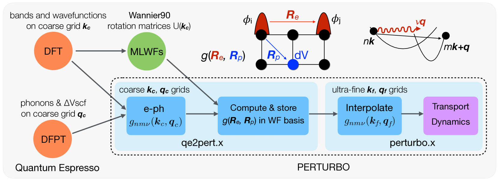
Figure 1: Workflow of the Perturbo code. Before running Perturbo, the user performs DFT calculations on the system of interest to obtain the Bloch states on a coarse $\bm{k}_{c}$-point grid and DFPT calculations to obtain the lattice dynamical properties and perturbation potentials on a coarse $\bm{q}_{c}$-point grid. The qe2pert.x executable of Perturbo computes the $e$-ph matrix elements on coarse $\bm{k}_{c}$- and $\bm{q}_{c}$-point grids, from which the $e$-ph matrix elements in the localized Wannier basis are obtained with the rotation matrices from Wannier90. The core executable perturbo.x is then employed to interpolate the band structure, phonon dispersion, and $e$-ph matrix elements on ultra-fine $\bm{k}_{f}$- and $\bm{q}_{f}$-point grids, and to perform charge transport and carrier dynamics calculations.

3 Capabilities and workflow

3.1 Code organization and capabilities

Perturbo contains two executables: a core program perturbo.x and the program qe2pert.x, which interfaces the QE code and perturbo.x, as shown in Fig. 1. The current release supports DFT and DFPT calculations with norm-conserving or ultrasoft pseudopotentials, with or without SOC; it also supports the Coulomb truncation for 2D materials [41]. The current features include calculations of:

1. Band structure, phonon dispersion, and $e$-ph matrix elements on arbitrary BZ grids or paths.

2. The $e$-ph scattering rates, relaxation times, and electron mean free paths for electronic states with any band and $\bm{k}$-point.

3. Electrical conductivity, carrier mobility, and Seebeck coefficient using the RTA or the iterative solution of the BTE.

4. Nonequilibrium dynamics, such as simulating the cooling and equilibration of excited carriers via interactions with phonons.

Several features of Perturbo, including the nonequilibrium dynamics, are unique and not available in other existing codes. Many additional features, currently being developed or tested, will be added to the list in future releases.
Perturbo stores most of the data and results in HDF5 file format, including all the main results of qe2pert.x, the TDF and other files generated in the transport calculations, and the nonequilibrium electron distribution computed in perturbo.x. The use of the HDF5 file format improves the portability of the results between different computing systems and is also convenient for post-processing using high-level languages, such as Python and Julia.
Installation and usage of Perturbo and an up-to-date list of supported features are documented in the user manual distributed along with the source code package, and can also be found on the code website [42].

3.2 Computational workflow

Figure 1 summarizes the workflow of Perturbo. Before running Perturbo, the user needs to carry out DFT and DFPT calculations with the QE code, and Wannier function calculations with Wannier90. In our workflow, we first carry out DFT calculations to obtain the band energies and Bloch wavefunctions on a coarse grid with points $\bm{k}_{c}$. A regular Monkhorst-Pack (MP) $\bm{k}_{c}$-point grid centered at $\Gamma$ and Bloch states for all $\bm{k}_{c}$-points in the first BZ are required. We then construct a set of Wannier functions from the Bloch wavefunctions using the Wannier90 code. Only the rotation matrices $\mathcal{U}$ that transform the DFT Bloch wavefunctions to the Wannier gauge and the center of the Wannier functions are required as input to Perturbo. We also perform DFPT calculations to obtain the dynamical matrices and $e$-ph perturbation potentials on a coarse MP grid with points $\bm{q}_{c}$. In the current version, the electron $\bm{k}_{c}$-point grid and phonon $\bm{q}_{c}$-point grid need to be commensurate. Since DFPT is computationally demanding, we carry out the DFPT calculations only for $\bm{q}_{c}$-points in the irreducible wedge of the BZ, and then obtain the dynamical matrices and perturbation potentials in the full BZ grid using space group and time reversal symmetries (see Sec. 4.1).
The executable qe2pert.x reads the results from DFT and DFPT calculations, including the Bloch states $|\psi_{n\bm{k}_{c}}\rangle$, dynamical matrices $D(\bm{q}_{c})$ and $e$-ph perturbation potentials $\partial_{\bm{q}_{c},\kappa\alpha}V$, and then computes the electron Hamiltonian in the Wannier basis [Eq. (17)] and the IFCs [Eq. (22)]. It also computes the $e$-ph matrix elements on coarse grids and transforms them to the localized Wannier basis using Eqs. (26)-(27). To ensure that the same Wannier functions are used for the electron Hamiltonian and $e$-ph matrix elements, we use the same DFT Bloch states $|\psi_{n\bm{k}_{c}}\rangle$ and $\mathcal{U}(\bm{k}_{c})$ matrices for the calculations in Eqs. (17) and (26)-(27). Following these preliminary steps, qe2pert.x outputs all the relevant data to an HDF5 file, which is the main input for perturbo.x.
The executable perturbo.x reads the data computed by qe2pert.x and carries out the transport and dynamics calculations discussed above. To accomplish these tasks, perturbo.x interpolates the band structure, phonon dispersion, and $e$-ph matrix elements on fine $\bm{k}$- and $\bm{q}$-point BZ grids, and uses these quantities in the various calculations.

4 Technical aspects

4.1 $e$-ph matrix elements on coarse grids

As discussed in Sec. 2.2.3, we compute directly the $e$-ph matrix elements in Eq. (26) using the DFT states on a coarse $\bm{k}_{c}$-point grid and the perturbation potentials on a coarse $\bm{q}_{c}$-point grid. It is convenient to rewrite Eq. (26) in terms of lattice-periodic quantities,

$$\tilde{g}_{mn}^{\kappa\alpha}\left(\bm{k}_{c},\bm{q}_{c}\right)=\left\langle u_{m{\bm{k}_{c}+\bm{q}_{c}}}\left|\partial_{\bm{q}_{c},\kappa\alpha}v\right|u_{n\bm{k}_{c}}\right\rangle,$$ (31)

where $|u_{n\bm{k}_{c}}\rangle$ is the lattice periodic part of the Bloch wavefunction and $\partial_{\bm{q}_{c},\kappa\alpha}v=e^{-i\bm{q}_{c}\cdot\bm{r}}\partial_{\bm{q}_{c},\kappa\alpha}V$ is the lattice-periodic perturbation potential. Since we compute only $|u_{n\bm{k}_{c}}\rangle$ on the coarse grid of the first BZ, $|u_{m\bm{k}_{c}+\bm{q}_{c}}\rangle$ may not be available because $\bm{k}_{c}+\bm{q}_{c}$ may be outside of the first BZ. However, by requiring the $\bm{q}_{c}$-point grid to be commensurate with and smaller than (or equal to) the $\bm{k}_{c}$-point grid, we can satisfy the relationship $\bm{k}_{c}+\bm{q}_{c}=\bm{k}^{\prime}_{c}+\bm{G}_{0}$, where $\bm{k}^{\prime}_{c}$ is on the coarse grid and $\bm{G}_{0}$ is a reciprocal lattice vector. Starting from $|u_{m\bm{k}^{\prime}_{c}}\rangle=\sum_{\bm{G}}c_{\bm{k}^{\prime}_{c}}(\bm{G})e^{i\bm{G}\cdot\bm{r}}$, we can thus obtain $|u_{m\bm{k}_{c}+\bm{q}_{c}}\rangle$ with negligible computational cost as

$$|u_{m\bm{k}_{c}+\bm{q}_{c}}\rangle=e^{-i\bm{G}_{0}\cdot\bm{r}}|u_{m\bm{k}^{\prime}_{c}}\rangle=\sum_{\bm{G}}c_{\bm{k}^{\prime}_{c}}(\bm{G})e^{i(\bm{G}-\bm{G}_{0})\cdot\bm{r}}.$$ (32)

The lattice-periodic perturbation potential $\partial_{\bm{q}_{c},\kappa\alpha}v$ consists of multiple terms, and can be divided into a local and a non-local part [43]. The non-local part includes the perturbation potentials due to the non-local terms of pseudopotentials, which typically includes the Kleinman-Bylander projectors and SOC terms. The local part includes the perturbations to the local part of the pseudopotentials as well as the self-consistent potential contribution. The latter, denoted as $\partial_{\bm{q}_{c},\kappa\alpha}v_{\rm sc}(\bm{r})$, accounts for the change in the Hartree and exchange-correlation potentials in response to the atomic displacements. While the pseudopotential contributions, both local and non-local, can be evaluated efficiently for all $\bm{q}_{c}$-points with the analytical formula given in Ref. [43], the self-consistent contribution $\partial_{\bm{q}_{c},\kappa\alpha}v_{\rm sc}(\bm{r})$ is computed and stored in real space using expensive DFPT calculations. This step is the main bottleneck of the entire $e$-ph computational workflow.
To improve the efficiency, we compute the self-consistent contribution with DFPT only for $\bm{q}_{c}$-points in the irreducible BZ wedge, and then unfold it to the equivalent points $\mathcal{S}\bm{q}_{c}$ in the full BZ using symmetry operations [44, 34]. For non-magnetic systems, $\partial_{\bm{q}_{c},\kappa\alpha}v_{\rm sc}(\bm{r})$ is a scalar function, so we can obtain the self-consistent contribution at $\mathcal{S}\bm{q}_{c}$ by rotating $\partial_{\bm{q}_{c},\kappa\alpha}v_{\rm sc}(\bm{r})$ [34]:

$$\partial_{\mathcal{S}\bm{q}_{c},\kappa\alpha}v_{\rm sc}(\bm{r})= \sum_{\kappa^{\prime}\beta}e^{i\bm{q}_{c}\cdot\bm{\tau}_{\kappa^{\prime}}-i\mathcal{S}\bm{q}_{c}\cdot\bm{\tau}_{\kappa}}$$ (33)

$$\times\left[\mathcal{S}^{-1}\right]_{\beta\alpha}\partial_{\bm{q}_{c},\kappa^{\prime}\beta}v_{\rm sc}\left(\{\mathcal{S}|\bm{t}\}^{-1}\bm{r}\right),$$

where $\{\mathcal{S}|\bm{t}\}$ is a space group symmetry operation of the crystal. A detailed derivation of Eq. (33) can be found in Appendix C of Ref. [34]. In addition to space group operations, time reversal symmetry is also used for non-magnetic systems via

$$\partial_{-\bm{q}_{c},\kappa\alpha}v_{\rm sc}(\bm{r})=[\partial_{\bm{q}_{c},\kappa\alpha}v_{\rm sc}(\bm{r})]^{*},$$ (34)

since the time reversal symmetry operator for a scalar function is the complex conjugation operator. We emphasize that Eq. (33) is only used to unfold the self-consistent contribution of the perturbation potential, while all the terms due to the pseudopotentials are computed directly, without using symmetry, for all the $\bm{q}_{c}$-points in the coarse grid.

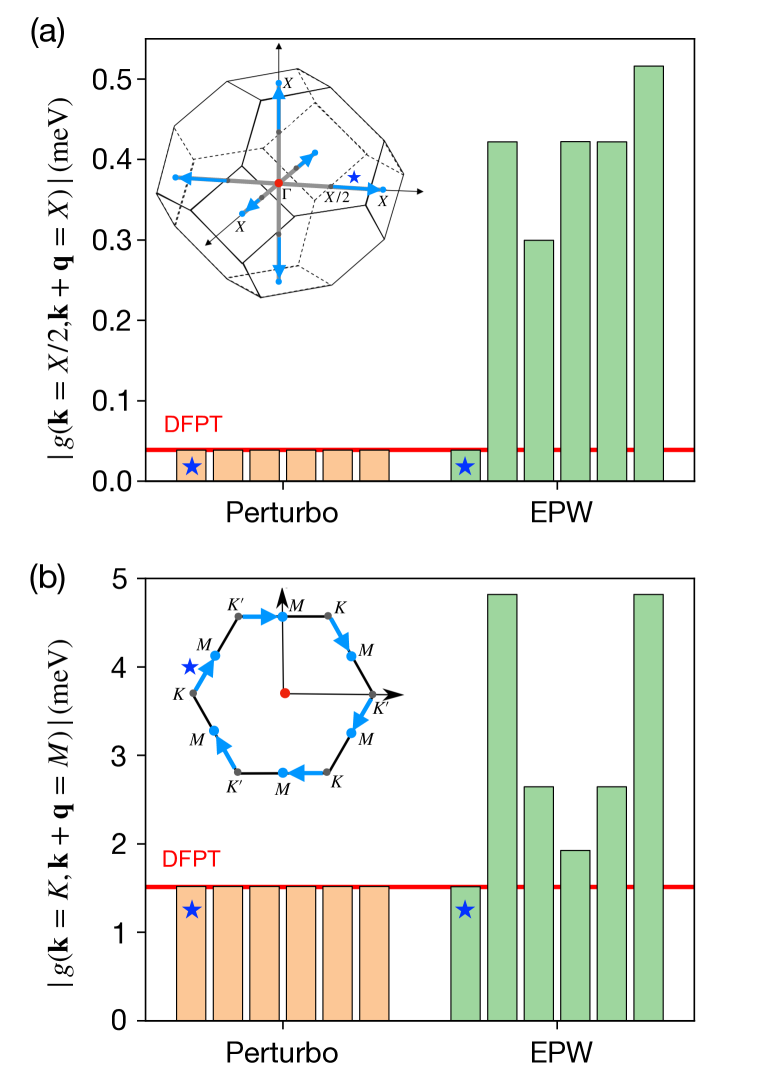
Figure 2: Absolute value of the gauge-invariant $e$-ph matrix elements, $\left|g\left(\bm{k},\bm{q}\right)\right|$ in Eq. (36), computed with Perturbo (orange) and EPW (green) in (a) silicon and (b) monolayer MoS₂. SOC is included in both cases. The six bars are $\left|g\left(\bm{k},\bm{q}\right)\right|$ values for six equivalent $(\bm{k},\bm{q})$ pairs connected by symmetry, which are shown as blue arrows in the inset. The result with $\bm{q}$ in the irreducible wedge (labeled with a blue star) is computed directly with the DFPT perturbation potential, while the others are obtained by applying symmetry operations either on the perturbation potentials (Perturbo) or on the wavefunctions (EPW). The red horizontal line shows the benchmark values computed directly from DFPT for all $(\bm{k},\bm{q})$ pairs.

An alternative approach to obtain the $e$-ph matrix elements in the full BZ starting from results in the irreducible wedge is to rotate the wavefunctions instead of the perturbation potential:

$$\langle u_{m{\bm{k}_{c}+\mathcal{S}\bm{q}_{c}}} |\partial_{\mathcal{S}\bm{q}_{c},\kappa\alpha}v|u_{n\bm{k}_{c}}\rangle=$$ (35)

$$\langle u_{m{\bm{k}_{c}+\mathcal{S}\bm{q}_{c}}}|\mathcal{D}_{\{\mathcal{S}|\bm{t}\}}^{\dagger}\partial_{\bm{q}_{c},\kappa\alpha}v\,\mathcal{D}_{\{\mathcal{S}|\bm{t}\}}|u_{n\bm{k}_{c}}\rangle,$$

where $\mathcal{D}_{\{\mathcal{S}|\bm{t}\}}$ is the symmetry operator acting on the wavefunction. In this approach (not employed in Perturbo), the perturbation potentials are needed only for $\bm{q}_{c}$ in the irreducible wedge [32]. It is important to keep in mind that the wavefunctions are spinors in non-collinear calculations, so the symmetry operators $\mathcal{D}_{\{\mathcal{S}|\bm{t}\}}$ should act both on the spatial coordinate and in spin space. Neglecting the rotation in spin space would lead to significant errors in the computed $e$-ph matrix elements, especially in calculations with SOC.
To benchmark our implementation, we compare the $e$-ph matrix elements obtained using symmetry operations to those from direct DFPT calculations. The absolute value of the $e$-ph matrix elements, $\left|g\left(\bm{k},\bm{q}\right)\right|$, is computed in gauge-invariant form for each phonon mode (with index $\nu$) by summing over bands:

$$\left|g_{\nu}\left(\bm{k},\bm{q}\right)\right|=\sqrt{\sum_{mn}\left|g_{mn\nu}\left(\bm{k},\bm{q}\right)\right|^{2}/N_{b}},$$ (36)

where $m$, $n$ are band indices for the selected $N_{b}$ bands. We perform the comparison with direct DFPT calculations for silicon and monolayer MoS₂ as examples of a bulk and a 2D material, respectively. We include SOC in both cases. For silicon, we choose $\bm{k}=X/2$, $\bm{k}+\bm{q}=X$ and compute $\left|g\left(\bm{k},\bm{q}\right)\right|$ in Eq. (36) using the four highest valence bands; for monolayer MoS₂, we choose $\bm{k}=K$, $\bm{k}+\bm{q}=M$ and compute $\left|g\left(\bm{k},\bm{q}\right)\right|$ for the two lowest conduction bands with 2D Coulomb truncation turned off. For both silicon and monolayer MoS₂, we compute $\left|g\left(\bm{k},\bm{q}\right)\right|$ for all the six equivalent $(\bm{k},\bm{q})$ pairs connected by space group and time reversal symmetry [see the inset of Fig. 2(a, b)]. As a benchmark, DFPT calculations are carried out to evaluate directly $\left|g\left(\bm{k},\bm{q}\right)\right|$ for all the six $(\bm{k},\bm{q})$ pairs. The results shown in Fig. 2 are for the lowest acoustic mode, though the results for the other modes show similar trends. The $\left|g\left(\bm{k},\bm{q}\right)\right|$ values computed with DFPT are identical for the six equivalent $(\bm{k},\bm{q})$ pairs (see the red horizontal line in Fig. 2), which is expected based on symmetry. In the Perturbo calculation, only the $(\bm{k},\bm{q})$ pair with $\bm{q}$ in the irreducible wedge is computed directly with the perturbation potential from DFPT, while results for the other five equivalent $(\bm{k},\bm{q})$ pairs are obtained by rotating the self-consistent perturbation potential. The results obtained with this approach match to a high accuracy the DFPT benchmark results, which validates the perturbation potential rotation approach implemented in Perturbo.
For comparison, we show in Fig. 2 the results from the alternative approach of rotating the wavefunctions, as implemented in the EPW code (version 5.2) [45]. Surprisingly, using the EPW code only the $\left|g\left(\bm{k},\bm{q}\right)\right|$ value for the $(\bm{k},\bm{q})$ pair containing the irreducible $\bm{q}$-point agrees with the DFPT benchmark, while all other $\left|g\left(\bm{k},\bm{q}\right)\right|$ values for $\bm{q}$-points obtained using symmetry operations show significant errors. We stress again that all the results in Fig. 2 are computed with SOC. We have verified that, in the absence of SOC, both Perturbo and EPW produce results in agreement with DFPT. The likely reason for the failure of EPW in this test is that in EPW the wavefunctions are rotated as scalars even in the presence of SOC, rather than as spinors as they should (that is, the rotation in spin space is missing). Further investigation of this discrepancy is critical, since the large errors in EPW for the coarse-grid $e$-ph matrix elements will propagate to the interpolated matrix elements on fine grids, giving incorrect results in calculations including SOC carried out with EPW [46].

4.2 Wigner-Seitz supercell for Wannier interpolation

As discussed in Sec. 2.2.1, the DFT Bloch states obtained at $\bm{k}_{c}$-points on a regular BZ grid are used to construct the Wannier functions. A discrete BZ grid implies a Born-von Karman (BvK) boundary condition in real space, so that an $N\times N\times N$ $\bm{k}_{c}$-point grid corresponds (for simple cubic, but extensions are trivial) to a BvK supercell of size $N\!a\times N\!a\times N\!a$, where $a$ is the lattice constant of the unit cell. If we regard the crystal as made up by an infinite set of BvK supercells at lattice vectors $\bm{T}_{e}$, we can label any unit cell in the crystal through its position $\bm{T}_{e}+\bm{R}_{e}$, where $\bm{R}_{e}$ is the unit cell position in the BvK supercell. Because of the BvK boundary condition, the Bloch wavefunctions are truly periodic functions over the BvK supercell, and the Wannier function $|n\bm{R}_{e}\rangle$ obtained using Eq. (15) is actually the superposition of images of the Wannier function in all the BvK supercells. Therefore, we can write $|n\bm{R}_{e}\rangle=\sum_{\bm{T}_{e}}|n,\bm{R}_{e}+\bm{T}_{e}\rangle^{0}$, where $|n,\bm{R}_{e}+\bm{T}_{e}\rangle^{0}$ denotes the image of the Wannier function in the BvK supercell at $\bm{T}_{e}$. Similarly, the electron Hamiltonian computed using Eq. (17) can be expressed as

$$H_{nn^{\prime}}(\bm{R}_{e})=\sum_{\bm{T}_{e}}H^{0}_{nn^{\prime}}(\bm{R}_{e}+\bm{T}_{e}).$$ (37)

The hopping matrix elements $H^{0}_{nn^{\prime}}(\bm{R}_{e}+\bm{T}_{e})$ usually decay rapidly as the distance between two image Wannier functions increases. The BvK supercell should be large enough to guarantee that only the hopping term between the two Wannier function images with the shortest distance is significant, while all other terms in the summation over $\bm{T}_{e}$ in Eq. (37) are negligible.
We use this “least-distance” principle to guide our choice of a set of $\bm{\tilde{R}}_{e}$ vectors for the Wannier interpolation. For each Hamiltonian matrix element labeled by $(n,n^{\prime},\bm{R}_{e})$ in Eq. (37), we compute the distance $d=|\bm{T}_{e}+\bm{R}_{e}+\bm{\tau}_{n^{\prime}}-\bm{\tau}_{n}|$, with $\bm{\tau}_{n}$ the position of the Wannier function center in the unit cell, and find the vector $\bm{T}_{e}^{0}$ giving the minimum distance. The set of vectors $\bm{\tilde{R}}_{e}=\bm{R}_{e}+\bm{T}_{e}^{0}$ is then selected to construct the Wigner-Seitz supercell used in the Wannier interpolation. We compute $H_{nn^{\prime}}(\bm{\tilde{R}}_{e})$ using Eq. (17) and use it to interpolate the band structure with Eq. (18). Note that the same strategy to construct the Wigner-Seitz supercell is also used in the latest version of Wannier90 [26].
Similarly, we choose a set of least-distance $\bm{\tilde{R}}_{p}$ vectors for the interpolation of the phonon dispersion, and separately determine least-distance $\bm{\tilde{R}}_{e}$ and $\bm{\tilde{R}}_{p}$ pairs for the interpolation of the $e$-ph matrix elements in Eqs. (27)-(28).

4.3 Brillouin zone sampling and integration

Several computational tasks carried out by Perturbo require integration in the BZ. Examples include scattering rate and TDF calculations, in Eqs. (8) and (13), respectively, and the iterative BTE solution in Eq. (10). In Perturbo, we adopt different BZ sampling and integration approaches for different kinds of calculations. For transport calculations, we use the tetrahedron method [23] for the integration over $\bm{k}$ in Eq. (13). We sample $\bm{k}$-points in the first BZ using a regular MP grid centered at $\Gamma$, and divide the BZ into small tetrahedra by connecting neighboring $\bm{k}$-points. The integration is first performed inside each tetrahedron, and the results are then added together to compute the BZ integral. To speed up these transport calculations, we set up a user-defined window spanning a small energy range (typically $\sim$0.5 eV) near the band edge in semiconductors or Fermi level in metals, and restrict the BZ integration to the $\bm{k}$-points with electronic states in the energy window. Since only states within a few times the thermal energy $k_{B}T$ of the band edge in semiconductors (or Fermi energy in metals) contribute to transport, including in the tetrahedron integration only $\bm{k}$-points in the relevant energy window greatly reduces the computational cost.
To compute the $e$-ph scattering rate for states with given bands and $\bm{k}$-points, we use the Monte Carlo integration as the default option. We sample random $\bm{q}$-points in the first BZ to carry out the summation over $\bm{q}$ in Eq. (8) and obtain the scattering rate. One can either increase the number of random $\bm{q}$-points until the scattering rate is converged or average the results from independent samples. Note that the energy broadening parameter used to approximate the $\delta$ function in Eq. (9) is important for the convergence of the scattering rate, so the convergence with respect to both the $\bm{q}$-point grid and broadening needs to be checked carefully [12]. Perturbo supports random sampling of the $\bm{q}$-points with either a uniform or a Cauchy distribution; a user-defined $\bm{q}$-point grid can also be specified in an external file and used in the calculation.
In the carrier dynamics simulations and in the iterative BTE solution in Eq. (10), the $\bm{k}$- and $\bm{q}$-points should both be on a regular MP grid centered at $\Gamma$. The two grids should be commensurate, with the size of the $\bm{q}$-point grid smaller than or equal to the size of the $\bm{k}$-point grid. This way, we satisfy the requirement in Eq. (10) that each $(\bm{k}$+$\bm{q})$-point is also on the $\bm{k}$-point grid. To perform efficiently the summation in Eq. (10) for all the $\bm{k}$-points, we organize the scattering probability in Eq. (9) using ($\bm{k}$, $\bm{q}$) pairs. We first determine a set of bands and $\bm{k}$-points for states inside the energy window. We then find all the possible scattering processes in which both the initial and final states are in the selected set of $\bm{k}$-points, and the phonon wave vector connecting the two states is on the $\bm{q}$-point grid. The scattering processes are indexed as ($\bm{k}$, $\bm{q}$) pairs; their corresponding $e$-ph matrix elements are computed and stored, and then retrieved from memory during the iteration process.

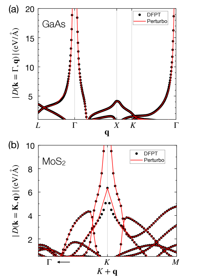
Figure 3: The $e$-ph deformation potential [see Eq. (38)] in (a) GaAs and (b) monolayer MoS₂ computed using Perturbo and compared with direct DFPT calculations for benchmarking.

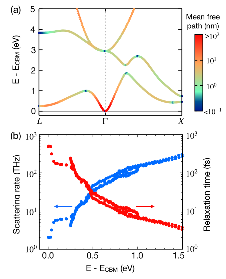
Figure 4: (a) Band structure of GaAs overlaid with a log-scale color map of the electron mean free paths computed at 300 K. (b) The $e$-ph scattering rates and their inverse, the relaxation times, for the electronic states in (a) given as a function of electron energy. The energy zero is the CBM.

5 Examples

In this section, we demonstrate the capabilities of the Perturbo code with a few representative examples, including calculations on a polar bulk material (GaAs), a 2D material with SOC (monolayer MoS₂), and an organic crystal (naphthalene) with a relatively large unit cell with 36 atoms.
The ground state and band structure are computed using DFT with a plane-wave basis with the QE code; this is a preliminary step for all Perturbo calculations, as discussed above. For GaAs, we use the same computational settings as in Ref. [12], namely a lattice constant of 5.556 Å  and a plane-wave kinetic energy cutoff of 72 Ry. For monolayer MoS₂, we use a 72 Ry kinetic energy cutoff, an experimental lattice constant of 3.16 Å and a layer-normal vacuum spacing of 17 Å. All calculations are carried out in the local density approximation of DFT using norm-conserving pseudopotentials. For MoS₂, we use fully relativistic norm-conserving pseudopotentials from Pseudo Dojo [47] to include SOC effects.

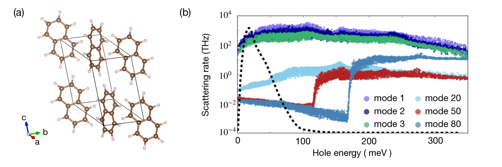
Figure 5: (a) Crystal structure of naphthalene, a prototypical organic molecular semiconductor with 36 atoms in the unit cell. (b) Mode-resolved $e$-ph scattering rates in naphthalene, computed at 300 K. Results are shown for three acoustic modes (1-3) associated with inter-molecular vibrations and three optical modes (20, 50, 80) associated with intra-molecular vibrations. The black dashed line represents the conductivity integrand in Eq. (12) and quantifies the relative contribution to transport as a function of electron energy. It is seen that only states within about 100 meV of the valence band maximum contribute to hole transport.

Lattice dynamical properties and the $e$-ph perturbation potential [see Eq. (25)] are computed on coarse $\bm{q}$-point grids of $8\times 8\times 8$ (GaAs) and $24\times 24\times 1$ (MoS₂) using DFPT as implemented in the QE code. We use the 2D Coulomb cutoff approach in DFPT for MoS₂ to remove the spurious interactions between layers [39]. For naphthalene, we use the same computational settings as in Ref. [15] for the DFT and DFPT calculations. Note that we only perform the DFPT calculations for the irreducible $\bm{q}$-points in the BZ grid, following which we extend the dynamical matrices to the entire BZ grid using space group and time reversal symmetry [see Eq. (33)] with our qe2pert.x routines.
The Wannier90 code is employed to obtain localized Wannier functions in each material. Only the centers of the Wannier functions and the rotation matrices $\mathcal{U}$ [see Eq. (16)] are read as input by qe2pert.x. The Wannier functions for GaAs are constructed using a coarse $8\times 8\times 8$ $\bm{k}$-point grid and $sp^{3}$ orbitals centered at the Ga and As atoms as an initial guess. For MoS₂, we construct 22 Wannier functions using a coarse $24\times 24\times 1$ $\bm{k}$-point grid and an initial guess of $d$ orbitals on Mo and $s$ orbitals on S atoms, using both spin up and spin down orbitals. For naphthalene, we construct two Wannier functions for the two highest valence bands using a coarse $\bm{k}$-point grid of $4\times 4\times 4$. The selected columns of density matrix (SCDM) approach [48] is employed to generate an initial guess automatically.
Following the workflow in Fig. 1, we compute the $e$-ph matrix elements on the coarse $\bm{k}$- and $\bm{q}$-point grids and obtain the $e$-ph matrix elements in the localized Wannier basis using qe2pert.x.

5.1 Interpolation of the $e$-ph matrix elements

It is important to check the accuracy of all interpolations before performing transport and carrier dynamics calculations. Perturbo provides routines and calculation modes to compute and output the interpolated band structure, phonon dispersion, and $e$-ph matrix elements, which should be compared to the same quantities computed using DFT and DFPT to verify that the interpolation has worked as expected. The comparison is straightforward for the band structure and phonon dispersion. Here we focus on validating the interpolation of the $e$-ph matrix elements, a point often overlooked in $e$-ph calculations. Since the $e$-ph matrix elements are gauge dependent, a direct comparison of $g_{mn\nu}\left(\bm{k},\bm{q}\right)$ from Perturbo and DFPT calculations is not meaningful. Instead, we compute the absolute value of the $e$-ph matrix elements, $\left|g_{\nu}\left(\bm{k},\bm{q}\right)\right|$, in the gauge-invariant form of Eq. (36), and the closely related “deformation potential”, which following Ref. [37] is defined as

$$D_{\nu}\left(\bm{k},\bm{q}\right)=\sqrt{2\omega_{\nu\bm{q}}M_{tot}}\left|g_{\nu}\left(\bm{k},\bm{q}\right)\right|/\hbar,$$ (38)

where $M_{tot}$ is the total mass of the atoms in the unit cell.
We show in Fig. 3 the deformation potentials for the bulk polar material GaAs and the 2D polar material MoS₂. For GaAs, we choose the $\Gamma$-point as the initial electron momentum $\bm{k}$, and vary the phonon wave vector $\bm{q}$ along a high-symmetry path, computing $D_{\nu}\left(\bm{k},\bm{q}\right)$ for the highest valence band. For MoS₂, we choose the $K$-point as the initial electron momentum and vary the final electron momentum $K+\bm{q}$ along a high-symmetry path, computing $D_{\nu}\left(\bm{k},\bm{q}\right)$ by summing over the two lowest conduction bands. In both cases, results are computed for all phonon modes. The respective polar corrections are included in both materials, which is crucial to accurately interpolate the $e$-ph matrix elements at small $\bm{q}$. The results show clearly that the $e$-ph interpolation works as expected, giving interpolated matrix elements in close agreement with direct DFPT calculations.

Figure 6: (a) Electron mobility in GaAs as a function of temperature, computed using the RTA and ITA methods and compared with experimental data [49, 50]. (b) Temperature dependent Seebeck coefficient in GaAs, computed for two different carrier concentrations. (c) Electron and hole mobilities in monolayer MoS₂ as a function of temperature, computed using the RTA and ITA.

5.2 Scattering rates and electron mean free paths

The perturbo.x routines can compute the $e$-ph scattering rate ($\Gamma_{n\bm{k}}$), relaxation time ($\tau_{n\bm{k}}=\Gamma_{n\bm{k}}^{-1}$), and electron mean free path ($L_{n\bm{k}}=\tau_{n\bm{k}}v_{n\bm{k}}$) for electronic states with any desired band and crystal momentum $\bm{k}$. Figure 4 shows the results for GaAs, in which we compute these quantities for the lowest few conduction bands and for $\bm{k}$-points along a high-symmetry path.
Carefully converging the scattering rate in Eq. (8) is important, but it can be far from trivial since in some cases convergence requires sampling millions of $\bm{q}$-points in the BZ. A widely applicable scheme is to sample random $\bm{q}$-points uniformly, and compute the scattering rates for increasing numbers of $\bm{q}$-points until the scattering rates are converged. However, uniform sampling can be nonoptimal in specific scenarios in which importance sampling can be used to speed up the convergence. For polar materials such as GaAs, the scattering rate for electronic states near the conduction band minimum (CBM) is dominated by small-$\bm{q}$ (intravalley) LO phonon scattering. In this case, importance sampling with a Cauchy distribution [12] that more extensively samples small $\bm{q}$ values can achieve convergence more effectively than uniform sampling. On the other hand, for electronic states in GaAs farther in energy from the band edges, the contributions to scattering are comparable for all phonon modes and momenta, so uniform sampling is effective because it avoids bias in the sampling. To treat optimally both sets of electronic states in polar materials like GaAs, we implement a polar split scheme in Perturbo, which is detailed in Ref. [12]. The scattering rates shown in Fig 4(b) are obtained with this approach.
 To analyze the dominant scattering mechanism for charge transport, it is useful to resolve the contributions to the total scattering rate from different phonon modes. Figure 5 shows the mode-resolved scattering rates for holes in naphthalene computed at 300 K [15]. A unit cell of naphthalene includes two molecules, for a total of 36 atoms [see Fig. 5(a)] and 108 phonon modes. Figure 5(b) shows the contribution to the scattering rate from the three acoustic phonon modes (modes 1$-$3), which are associated with inter-molecular vibrations. The contributions from three optical modes (modes 20, 50, 80) associated with intra-molecular atomic vibrations are also shown. In the relevant energy range for transport, as shown by the dashed line in Fig. 5(b), the inter-molecular modes dominate hole carrier scattering. This analysis is simple to carry out in Perturbo because the code can output the TDF and mode-resolved scattering rates.

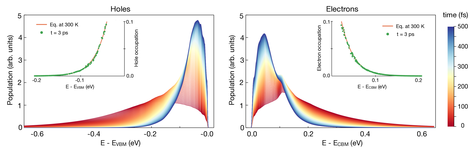
Figure 7: Hot carrier cooling simulation in silicon, for holes (left panel) and electrons (right panel). The time evolution of the carrier population $p(E,t)$ in Eq. (39) is shown, with the simulation time $t$ color-coded. The carrier occupations $f_{n\bm{k}}(t)$ at $t$ = 3 ps are compared in the inset with the equilibrium Fermi-Dirac distribution at 300 K (red curve) for the same carrier concentration.

5.3 Charge transport

We present charge transport calculations for GaAs and monolayer MoS₂ as examples of a bulk and 2D material, respectively. Since both materials are polar, the polar corrections to the $e$-ph matrix elements are essential, as shown in Fig. 3. For MoS₂, we include SOC in the calculation since it plays an important role. In MoS₂, SOC splits the states near the valence band edge, so its inclusion has a significant impact on the $e$-ph scattering rates and mobility for hole carriers. The transport properties can be computed in Perturbo either within the RTA or with the iterative solution of the linearized BTE. In the RTA, one can use pre-computed state-dependent scattering rates (see Sec. 5.2) or compute the scattering rates on the fly during the transport calculation using regular MP $\bm{k}$- and $\bm{q}$-point grids. In some materials, the RTA is inadequate and the more accurate iterative solution of the BTE in Eq. (10) is required. Perturbo implements an efficiently parallelized routine to solve the BTE iteratively (see Sec. 6).
Figure 6(a) shows the computed electron mobility in GaAs as a function of temperature and compares results obtained with the RTA and the iterative approach (ITA). The calculation uses a carrier concentration of $n_{c}\!=\!10^{17}$ cm^-3; we have checked that the mobility is almost independent of $n_{c}$ below 10¹⁸ cm^-3. We perform the calculation using an ultra-fine BZ grid of $600\times 600\times 600$ for both $\bm{k}$- and $\bm{q}$-points, and employ a small (5 meV) Gaussian broadening to approximate the $\delta$ function in the $e$-ph scattering terms in Eq. (9). To reduce the computational cost, we select a 200 meV energy window near the CBM, which covers the entire energy range relevant for transport. In GaAs, the ITA gives a higher electron mobility than the RTA, as shown in Fig. 6(a), and this discrepancy increases with temperature. The temperature dependence of the electron mobility is also slightly different in the RTA and ITA results. The RTA calculation is in better agreement with experimental data [49, 50] than results from the more accurate ITA. Careful analysis, carried out elsewhere [51], shows that correcting the band structure [52] to obtain an accurate effective mass and including two-phonon scattering processes [51] are both essential to obtain ITA results in agreement with experiment.
The Seebeck coefficient can be computed at negligible cost as a post-processing step of the mobility calculation. Figure 6(b) shows the temperature dependent Seebeck coefficient in GaAs, computed using the ITA at two different carrier concentrations. The computed value at 300 K and $n_{c}\!=\!10^{18}$ cm^-3 is about 130 $\mu$V/K, in agreement with the experimental value of $\sim$150 $\mu$V/K [53]. Our results also show that the Seebeck coefficient increases with temperature and for decreasing carrier concentrations (here, we tested $n_{c}\!=\!10^{17}$ cm^-3), consistent with experimental data near room temperature [53, 54]. Note that the phonon occupations are kept fixed at their equilibrium value in our calculations, so the phonon drag effect, which is particularly important at low temperature, is neglected, and only the diffusive contribution to the Seebeck coefficient is computed. To include phonon drag one needs to include nonequilibrium phonon effects in the Seebeck coefficient calculation. While investigating the coupled dynamics of electrons and phonons remains an open challenge in first-principles calculations [22, 55], we are developing an approach to time-step the coupled electron and phonon BTEs, and plan to make it available in a future version of Perturbo.
Figure 6(c) shows the electron and hole mobilities in monolayer MoS₂, computed for a carrier concentration of $2\times 10^{12}$ cm^-2 and for temperatures between 150$-$350 K. A fine BZ grid of $180\times 180\times 1$ is employed for both $\bm{k}$- and $\bm{q}$-points. Different from GaAs, the RTA and ITA give very close results for both the electron and hole mobilities, with only small differences at low temperature. The computed electron mobility at room temperature is about 168 cm²/V s, in agreement with the experimental value of 150 cm²/V s [56]; the computed hole mobility at 300 K is about 20 cm²/V s.

5.4 Ultrafast dynamics

We demonstrate nonequilibrium ultrafast dynamics simulations using hot carrier cooling in silicon as an example. Excited (so-called “hot”) carriers can be generated in a number of ways in semiconductors, including injection from a contact or excitation with light. In a typical scenario, the excited carriers relax to the respective band edge in a sub-picosecond time scale by emitting phonons. While ultrafast carrier dynamics has been investigated extensively in experiments, for example with ultrafast optical spectroscopy, first-principles calculations of ultrafast dynamics, and in particular of hot carriers in the presence of $e$-ph interactions, are a recent development [19, 14, 57, 58].
We perform a first-principles simulation of hot carrier cooling in silicon. We use a lattice constant of 5.389 Å for DFT and DFPT calculations, which are carried out within the local density approximation and with norm-conserving pseudopotentials. Following the workflow in Fig. 1, we construct 8 Wannier functions using $sp^{3}$ orbitals on Si atoms as an initial guess, and obtain the $e$-ph matrix elements in the Wannier basis using coarse $8\times 8\times 8$ $\bm{k}$- and $\bm{q}$-point grids.

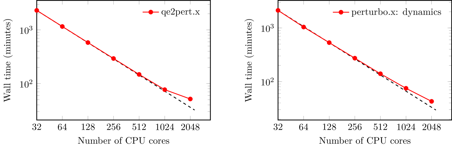
Figure 8: Performance scaling with the number of CPU cores of qe2pert.x and perturbo.x. The black dashed line indicates the ideal linear scaling. For perturbo.x, we show the performance of the carrier dynamics simulation, which is the most time-consuming task of perturbo.x.

Starting from the $e$-ph matrix elements in the Wannier basis, the electron Hamiltonian, and interatomic force constants computed by qe2pert.x, we carry out hot carrier cooling simulations, separately for electron and hole carriers, using a fine $\bm{k}$-point grid of $100\times 100\times 100$ for the electrons (or holes) and a $50\times 50\times 50$ $\bm{q}$-point grid for the phonons. A small Gaussian broadening of 8 meV is employed to approximate the $\delta$ function in the $e$-ph scattering terms in Eq. (9). The phonon occupations are kept fixed at their equilibrium value at 300 K. We set the initial electron and hole occupations to hot Fermi-Dirac distributions at 1500 K, each with a chemical potential corresponding to a carrier concentration of 10¹⁹ cm^-3. We explicitly time-step the BTE in Eq. (4) (with external electric field set to zero) using the RK4 method with a small time step of 1 fs, and obtain nonequilibrium carrier occupations $f_{n\bm{k}}(t)$ as a function of time $t$ up to 3 ps, for a total of 3,000 time steps. The calculation takes only about 2.5 hours using 128 CPU cores due to the efficient parallelization (see Sec. 6). To visualize the time evolution of the carrier distributions, we compute the BZ averaged energy-dependent carrier population,

$$p(E,t)=\sum_{n\bm{k}}f_{n\bm{k}}(t)\delta(\varepsilon_{n\bm{k}}-E),$$ (39)

using the tetrahedron integration method. The carrier population $p(E,t)$ characterizes the time-dependent energy distribution of the carriers.
Figure 7 shows the evolution of the electron and hole populations due to $e$-ph scattering. For both electrons and holes, the high-energy tail in the initial population decays rapidly as the carriers quickly relax toward energies closer to the band edge within 500 fs. The carrier concentration is conserved during the simulation, validating the accuracy of our RK4 implementation to time-step the BTE. The hole relaxation is slightly faster than the electron relaxation in silicon, as shown in Fig. 7. The sub-picosecond time scale we find for the hot carrier cooling is consistent with experiment and with previous calculations using a simplified approach [19]. Although the hot carriers accumulate near the band edge in a very short time, it takes longer for the carriers to fully relax to a 300 K thermal equilibrium distribution, up to several picoseconds in our simulation. We show in the inset of Fig. 7 that the carrier occupations $f_{n\bm{k}}$ at 3 ps reach the correct long-time limit for our simulation, namely an equilibrium Fermi-Dirac distribution at the 300 K lattice temperature. Since we keep the phonon occupations fixed and neglect phonon-phonon scattering, hot-phonon effects are ignored in our simulation. Similarly, electron-electron scattering, which is typically important at high carrier concentrations or in metals, is also not included in the current version of the code. Electron-electron scattering and coupled electron and phonon dynamics (including phonon-phonon collisions) are both under development.

6 Parallelization and performance

Transport calculations and ultrafast dynamics simulations on large systems can be computationally demanding and require a large amount of memory. Efficient parallelization is critical to run these calculations on high-performance computing (HPC) systems. To fully take advantage of the typical HPC architecture, we implement a hybrid MPI and OpenMP parallelization, which combines distributed memory parallelization among different nodes using MPI and on-node shared memory parallelization using OpenMP.
For small systems, we observe a similar performance by running Perturbo on a single node in either pure MPI or pure OpenMP modes, or in hybrid MPI plus OpenMP mode. However, for larger systems with several atoms to tens of atoms in the unit cell, running on multiple nodes with MPI plus OpenMP parallelization significantly improves the performance and leads to a better scaling with CPU core number. Compared to pure MPI, the hybrid MPI plus OpenMP scheme reduces communication needs and memory consumption, and improves load balance. We demonstrate the efficiency of our parallelization strategy using two examples: computing $e$-ph matrix elements on coarse grids, which is the most time-consuming task of qe2pert.x, and simulating nonequilibrium carrier dynamics, the most time-consuming task of perturbo.x.
For the calculation of $e$-ph matrix elements on coarse grids [see Eq. (31)], our implementation uses MPI parallelization for $\bm{q}_{c}$-points and OpenMP parallelization for $\bm{k}_{c}$-points. We distribute the $\bm{q}_{c}$-points among the MPI processes, so that each MPI process either reads the self-consistent perturbation potential from file (if $\bm{q}_{c}$ is in the irreducible wedge) or computes it from the perturbation potential of the corresponding irreducible point using Eq. (33). Each MPI process then computes $g(\bm{k}_{c},\bm{q}_{c})$ for all the $\bm{k}_{c}$-points with OpenMP parallelization.
For carrier dynamics simulations, the $\bm{k}$-points on the fine grid are distributed among MPI processes to achieve an optimal load balance. Each process finds all the possible scattering channels involving its subset of $\bm{k}$-points, and stores these scattering processes locally as $(\bm{k},\bm{q})$ pairs. One can equivalently think of this approach as distributing the $(\bm{k},\bm{q})$ pairs for the full $\bm{k}$-point set among MPI processes. After this step, we use OpenMP parallelization over local $(\bm{k},\bm{q})$ pairs to compute the $e$-ph matrix elements and perform the scattering integral. The iterative BTE in Eq. (10) is also parallelized with the same approach. This parallelization scheme requires minimum communication among MPI processes; for example, only one MPI reduction operation is required to collect the contributions from different processes for the integration in Eq. (10).
We test the parallelization performance of qe2pert.x and perturbo.x using calculations on MoS₂ and silicon as examples (see Sec. 5 for the computational details). We run the carrier dynamics simulation on silicon using the Euler method with a time step of 1 fs and a total simulation time of 50 ps, for a total of 50,000 steps. The tests are performed on the Cori system of the National Energy Research Scientific Computing center (NERSC). We use the Intel Xeon “Haswell” processor nodes, where each node has 32 CPU cores with a clock frequency of 2.3 GHz.
Figure 8 shows the wall time of the test calculations using different numbers of CPU cores. Both qe2pert.x and perturbo.x show rather remarkable scaling that is close to the ideal linear-scaling limit up to 1,024 CPU cores. The scaling of qe2pert.x for 2,048 CPU cores is less than ideal mainly because each MPI process has an insufficient computational workload, so that communication and I/O become a bottleneck. The current release uses the serial HDF5 library, so after computing $g(\bm{k}_{c},\bm{q}_{c})$, the root MPI process needs to collect $g(\bm{k}_{c},\bm{q}_{c})$ from different processes and write them to disk (or vice versa when loading data), which is a serial task that costs $\sim$14% of the total wall time when using 2048 CPU cores. Parallel I/O using the parallel HDF5 library could further improve the performance and overall scaling in this massively parallel example. We plan to work on this and related improvements to I/O in future releases.

7 Conclusions and outlook

In conclusion, we present our software, Perturbo, for first-principles calculations of charge transport properties and simulation of ultrafast carrier dynamics in bulk and 2D materials. The software contains an interface program to read results from DFT and DFPT calculations from the QE code. The core program of Perturbo performs various computational tasks, such as computing $e$-ph scattering rates, electron mean free paths, electrical conductivity, mobility, and the Seebeck coefficient. The code can also simulate the nonequilibrium dynamics of excited electrons. Wannier interpolation and symmetry are employed to greatly reduce the computational cost. SOC and the polar corrections for bulk and 2D materials are supported and have been carefully tested. We demonstrate these features with representative examples. We also show the highly promising scaling of Perturbo on massively parallel HPC architectures, owing to its effective implementation of hybrid MPI plus OpenMP parallelization.
Several features are currently under development for the next major release, including spin-phonon relaxation times and spin dynamics [8], transport calculations in the large polaron regime using the Kubo formalism [59], and charge transport and ultrafast dynamics for coupled electrons and phonons, among others. As an alternative to Wannier functions, interpolation using atomic orbitals [34] will also be supported in a future release. We will extend the interface program to support additional external codes, such as the TDEP software for temperature-dependent lattice dynamical calculations [13, 60].

References

- Rossi and Kuhn [2002] F. Rossi, T. Kuhn, Theory of ultrafast phenomena in photoexcited semiconductors, Rev. Mod. Phys. 74 (3) (2002) 895–950.
- Ulbricht et al. [2011] R. Ulbricht, E. Hendry, J. Shan, T. F. Heinz, M. Bonn, Carrier dynamics in semiconductors studied with time-resolved terahertz spectroscopy, Rev. Mod. Phys. 83 (2) (2011) 543–586.
- Egger et al. [2018] D. A. Egger, A. Bera, D. Cahen, G. Hodes, T. Kirchartz, L. Kronik, et al., What remains unexplained about the properties of halide perovskites?, Adv. Mater. 30 (20) (2018) 1800691.
- Baroni et al. [2001] S. Baroni, S. de Gironcoli, A. Dal Corso, P. Giannozzi, Phonons and related crystal properties from density-functional perturbation theory, Rev. Mod. Phys. 73 (2) (2001) 515–562.
- Giannozzi et al. [2009] P. Giannozzi, S. Baroni, N. Bonini, M. Calandra, R. Car, et al., QUANTUM ESPRESSO: a modular and open-source software project for quantum simulations of materials, J. Phys.: Condens. Matter 21 (39) (2009) 395502.
- Giannozzi et al. [2017] P. Giannozzi, O. Andreussi, T. Brumme, O. Bunau, M. B. Nardelli, et al., Advanced capabilities for materials modelling with QUANTUM ESPRESSO, J. Phys.: Condens. Matter 29 (46) (2017) 465901.
- Ziman [2007] J. M. Ziman, Electrons and phonons: The theory of transport phenomena in solids, Oxford University Press, New York, 2007.
- Park et al. [2020] J. Park, J.-J. Zhou, M. Bernardi, Spin-phonon relaxation times in centrosymmetric materials from first principles, Phys. Rev. B 101 (2020) 045202.
- Lu et al. [2019a] I.-T. Lu, J.-J. Zhou, M. Bernardi, Efficient ab initio calculations of electron-defect scattering and defect-limited carrier mobility, Phys. Rev. Mater. 3 (2019a) 033804.
- Lu et al. [2019b] I.-T. Lu, J. Park, J.-J. Zhou, M. Bernardi, Ab initio electron-defect interactions using Wannier functions, arXiv:1910.14516 [cond-mat.mtrl-sci] .
- Chen et al. [2019] H.-Y. Chen, V. A. Jhalani, M. Palummo, M. Bernardi, Ab initio calculations of exciton radiative lifetimes in bulk crystals, nanostructures, and molecules, Phys. Rev. B 100 (2019) 075135.
- Zhou and Bernardi [2016] J.-J. Zhou, M. Bernardi, Ab initio electron mobility and polar phonon scattering in GaAs, Phys. Rev. B 94 (20) (2016) 201201(R).
- Zhou et al. [2018] J.-J. Zhou, O. Hellman, M. Bernardi, Electron-phonon scattering in the presence of soft modes and electron mobility in perovskite from first principles, Phys. Rev. Lett. 121 (22) (2018) 226603.
- Jhalani et al. [2017] V. A. Jhalani, J.-J. Zhou, M. Bernardi, Ultrafast hot carrier dynamics in GaN and its impact on the efficiency droop, Nano Lett. 17 (8) (2017) 5012–5019.
- Lee et al. [2018] N.-E. Lee, J.-J. Zhou, L. A. Agapito, M. Bernardi, Charge transport in organic molecular semiconductors from first principles: The bandlike hole mobility in a naphthalene crystal, Phys. Rev. B 97 (11) (2018) 115203.
- Bernardi [2016] M. Bernardi, First-principles dynamics of electrons and phonons, Eur. Phys. J. B 89 (11) (2016) 239.
- Madsen and Singh [2006] G. K. H. Madsen, D. J. Singh, BoltzTraP. A code for calculating band-structure dependent quantities, Comput. Phys. Commun. 175 (1) (2006) 67–71.
- Pizzi et al. [2014] G. Pizzi, D. Volja, B. Kozinsky, M. Fornari, N. Marzari, BoltzWann: A code for the evaluation of thermoelectric and electronic transport properties with a maximally-localized Wannier functions basis, Comput. Phys. Commun. 185 (1) (2014) 422–429.
- Bernardi et al. [2014] M. Bernardi, D. Vigil-Fowler, J. Lischner, J. B. Neaton, S. G. Louie, Ab initio study of hot carriers in the first picosecond after sunlight absorption in silicon, Phys. Rev. Lett. 112 (2014) 257402.
- Mahan [2000] G. D. Mahan, Many-particle physics, Springer US, 3rd edn., 2000.
- Li [2015] W. Li, Electrical transport limited by electron-phonon coupling from Boltzmann transport equation: An ab initio study of Si, Al, and , Phys. Rev. B 92 (7) (2015) 075405.
- Fiorentini and Bonini [2016] M. Fiorentini, N. Bonini, Thermoelectric coefficients of -doped silicon from first principles via the solution of the Boltzmann transport equation, Phys. Rev. B 94 (8) (2016) 085204.
- Blöchl et al. [1994] P. E. Blöchl, O. Jepsen, O. K. Andersen, Improved tetrahedron method for Brillouin-zone integrations, Phys. Rev. B 49 (23) (1994) 16223–16233.
- Marzari et al. [2012] N. Marzari, A. A. Mostofi, J. R. Yates, I. Souza, D. Vanderbilt, Maximally localized Wannier functions: Theory and applications, Rev. Mod. Phys. 84 (4) (2012) 1419–1475.
- Mostofi et al. [2014] A. A. Mostofi, J. R. Yates, G. Pizzi, Y.-S. Lee, I. Souza, D. Vanderbilt, N. Marzari, An updated version of wannier90: A tool for obtaining maximally-localised Wannier functions, Comput. Phys. Commun. 185 (8) (2014) 2309–2310.
- Pizzi et al. [2020] G. Pizzi, V. Vitale, R. Arita, S. Blügel, F. Freimuth, G. Géranton, M. Gibertini, D. Gresch, C. Johnson, T. Koretsune, et al., Wannier90 as a community code: new features and applications, J. Phys.: Condens. Matter 32 (16) (2020) 165902.
- Wang et al. [2006] X. Wang, J. R. Yates, I. Souza, D. Vanderbilt, Ab initio calculation of the anomalous Hall conductivity by Wannier interpolation, Phys. Rev. B 74 (2006) 195118.
- Souza et al. [2001] I. Souza, N. Marzari, D. Vanderbilt, Maximally localized Wannier functions for entangled energy bands, Phys. Rev. B 65 (3) (2001) 035109.
- Yates et al. [2007] J. R. Yates, X. Wang, D. Vanderbilt, I. Souza, Spectral and Fermi surface properties from Wannier interpolation, Phys. Rev. B 75 (19) (2007) 195121.
- Born and Huang [1954] M. Born, K. Huang, Dynamical theory of crystal lattices, Clarendon press, 1954.
- Gonze and Lee [1997] X. Gonze, C. Lee, Dynamical matrices, Born effective charges, dielectric permittivity tensors, and interatomic force constants from density-functional perturbation theory, Phys. Rev. B 55 (16) (1997) 10355–10368.
- Giustino et al. [2007] F. Giustino, M. L. Cohen, S. G. Louie, Electron-phonon interaction using Wannier functions, Phys. Rev. B 76 (16) (2007) 165108.
- Calandra et al. [2010] M. Calandra, G. Profeta, F. Mauri, Adiabatic and nonadiabatic phonon dispersion in a Wannier function approach, Phys. Rev. B 82 (16) (2010) 165111.
- Agapito and Bernardi [2018] L. A. Agapito, M. Bernardi, Ab initio electron-phonon interactions using atomic orbital wave functions, Phys. Rev. B 97 (23) (2018) 235146.
- Gonze et al. [1994] X. Gonze, J.-C. Charlier, D. Allan, M. Teter, Interatomic force constants from first principles: The case of -quartz, Phys. Rev. B 50 (1994) 13035(R).
- Fröhlich [1954] H. Fröhlich, Electrons in lattice fields, Adv. Phys. 3 (11) (1954) 325–361.
- Sjakste et al. [2015] J. Sjakste, N. Vast, M. Calandra, F. Mauri, Wannier interpolation of the electron-phonon matrix elements in polar semiconductors: Polar-optical coupling in GaAs, Phys. Rev. B 92 (5) (2015) 054307.
- Verdi and Giustino [2015] C. Verdi, F. Giustino, Fröhlich electron-phonon vertex from first principles, Phys. Rev. Lett. 115 (17) (2015) 176401.
- Sohier et al. [2016] T. Sohier, M. Calandra, F. Mauri, Two-dimensional Fröhlich interaction in transition-metal dichalcogenide monolayers: Theoretical modeling and first-principles calculations, Phys. Rev. B 94 (2016) 085415.
- Sohier et al. [2017a] T. Sohier, M. Gibertini, M. Calandra, F. Mauri, N. Marzari, Breakdown of optical phonons’ splitting in two-dimensional materials, Nano Lett. 17 (6) (2017a) 3758–3763.
- Sohier et al. [2017b] T. Sohier, M. Calandra, F. Mauri, Density functional perturbation theory for gated two-dimensional heterostructures: Theoretical developments and application to flexural phonons in graphene, Phys. Rev. B 96 (2017b) 075448.
- per [????] The Perturbo website, https://perturbo-code.github.io
- Dal Corso [2001] A. Dal Corso, Density-functional perturbation theory with ultrasoft pseudopotentials, Phys. Rev. B 64 (23) (2001) 235118.
- Maradudin and Vosko [1968] A. A. Maradudin, S. H. Vosko, Symmetry properties of the normal vibrations of a crystal, Rev. Mod. Phys. 40 (1) (1968) 1–37.
- Poncé et al. [2016] S. Poncé, E. R. Margine, C. Verdi, F. Giustino, EPW: Electron–phonon coupling, transport and superconducting properties using maximally localized Wannier functions, Comput. Phys. Commun. 209 (2016) 116–133.
- Gaddemane et al. [2019] G. Gaddemane, S. Gopalan, M. Van de Put, M. V. Fischetti, Limitations of ab initio methods to predict the electronic-transport properties of two-dimensional materials: The computational example of 2H-phase transition metal dichalcogenides, arXiv:1912.03795 [cond-mat.mtrl-sci] .
- van Setten et al. [2018] M. J. van Setten, M. Giantomassi, E. Bousquet, M. J. Verstraete, D. R. Hamann, et al., The PseudoDojo: Training and grading a 85 element optimized norm-conserving pseudopotential table, Comput. Phys. Commun. 226 (2018) 39–54.
- Damle et al. [2017] A. Damle, L. Lin, L. Ying, SCDM-k: Localized orbitals for solids via selected columns of the density matrix, J. Comput. Phys. 334 (2017) 1–15.
- Blood [1972] P. Blood, Electrical properties of -type epitaxial GaAs at high temperatures, Phys. Rev. B 6 (6) (1972) 2257–2261.
- Nichols et al. [1980] K. H. Nichols, C. M. L. Yee, C. M. Wolfe, High-temperature carrier transport in -type epitaxial GaAs, Solid-State Electron. 23 (2) (1980) 109–116.
- Lee et al. [2019] N.-E. Lee, J.-J. Zhou, H.-Y. Chen, M. Bernardi, Next-to-leading order ab initio electron-phonon scattering, arXiv:1903.08261 [cond-mat.mes-hall] .
- Ma et al. [2018] J. Ma, A. S. Nissimagoudar, W. Li, First-principles study of electron and hole mobilities of Si and GaAs, Phys. Rev. B 97 (4) (2018) 045201.
- Madelung et al. [2002] O. Madelung, U. Rössler, M. Schulz (Eds.), Semiconductors, vol. 41A1, Springer, Berlin, 2002.
- Homm et al. [2008] G. Homm, P. J. Klar, J. Teubert, W. Heimbrodt, Seebeck coefficients of n-type (Ga,In)(N,As), (B,Ga,In)As, and GaAs, Appl. Phys. Lett. 93 (4) (2008) 042107.
- Protik and Broido [2019] N. H. Protik, D. A. Broido, Coupled transport of phonons and carriers in semiconductors, arXiv:1911.02916 [cond-mat.mtrl-sci] .
- Yu et al. [2016] Z. Yu, Z.-Y. Ong, Y. Pan, Y. Cui, R. Xin, Y. Shi, et al., Realization of room-temperature phonon-limited carrier transport in monolayer MoS2 by dielectric and carrier screening, Adv. Mater. 28 (3) (2016) 547–552.
- Sadasivam et al. [2017] S. Sadasivam, M. K. Y. Chan, P. Darancet, Theory of thermal relaxation of electrons in semiconductors, Phys. Rev. Lett. 119 (2017) 136602.
- Molina-Sánchez et al. [2017] A. Molina-Sánchez, D. Sangalli, L. Wirtz, A. Marini, Ab initio calculations of ultrashort carrier dynamics in two-dimensional materials: Valley depolarization in single-layer WSe2, Nano Lett. 17 (8) (2017) 4549–4555.
- Zhou and Bernardi [2019] J.-J. Zhou, M. Bernardi, Predicting charge transport in the presence of polarons: The beyond-quasiparticle regime in , Phys. Rev. Research 1 (2019) 033138.
- Hellman et al. [2013] O. Hellman, P. Steneteg, I. A. Abrikosov, S. I. Simak, Temperature dependent effective potential method for accurate free energy calculations of solids, Phys. Rev. B 87 (10) (2013) 104111.