Employing Non-Markovian effects to improve the performance of a quantum Otto refrigerator

Abstract

The extension of quantum thermodynamics to situations that go beyond standard thermodynamic settings comprises an important and interesting aspect of its development. One such situation is the analysis of the thermodynamic consequences of structured environments that induce a non-Markovian dynamics. We study a quantum Otto refrigerator where the standard Markovian cold reservoir is replaced by a specific engineered cold reservoir which may induce a Markovian or non-Markovian dynamics on the quantum refrigerant system. The two dynamical regimes can be interchanged by varying the coupling between the refrigerant and the reservoir. An increase of non-Markovian effects will be related to an increase of the coupling strength, which in turn will make the energy stored in the interaction Hamiltonian, the interaction energy, increasingly relevant. We show how the figures of merit, the coefficient of performance and the cooling power, change for non-negligible interaction energies, discussing how neglecting this effect would lead to an overestimation of the refrigerator performance. Finally, we also consider a numerical simulation of a spin quantum refrigerator with experimentally feasible parameters to better illustrate the non-Markovian effects induced by the engineered cold reservoir. We argue that a moderate non-Markovian dynamics performs better than either a Markovian or a strong non-Markovian regime of operation.

I Introduction

The theoretical description of thermal machines was fundamental to the development of classical thermodynamics, providing an operational understanding of the second law as established by Thomson (Lord Kelvin) (Thomson1851, ) and Carnot (Carnot, ). Moreover, the thermodynamic characterization of heat engines and refrigerators is essential to engineering since it provides tools for estimating the performance of such machines (=0000C7engelbook2015, ; Kondepudibook2015, ). In the same perspective, it is expected that the development of quantum thermodynamics will play a similar role in quantum engineering to the development of quantum technologies (Dowling2003, ; Georgescu2012, ; Jones2013, ).

Quantum thermal machines are excellent platforms to test results from quantum thermodynamics (Esposito2009, ; Campisi2011, ; Kosloff2013, ; GelbwaserKlimovsky2015, ; Millen2016, ; Vinjanampathya2016, ; Ribeiro2016, ), transforming heat into work and vice versa. In the quantum heat engine configuration, the purpose is to extract the largest amount of work by absorbing the least amount of heat from a hot source. On the other hand, in the quantum refrigerator setting, the goal is to absorb the largest amount of heat from a cold source by injecting the least amount of work into the refrigerant. The performance of the former is characterized by the thermodynamic efficiency and the power output, while that of the latter is characterized by the coefficient of performance (COP) and the cooling power. The theoretical underpinnings of the description of quantum thermal machines dates back to the late 1950s with the early works of Scovil and Schulz-DuBois (Scovil1959, ; Geusic1967, ). Since then, several theoretical investigations on quantum heat engines and refrigerators have been carried out (Alicki1979, ; Kosloff1984, ; Geva1992, ; Geva1992b, ; Geva1996, ; Kosloff2000, ; Scully2002, ; S=0000E1nchezSalas2004, ; Feldmann2006, ; Ting2006, ; Quan2007, ; Allahverdyan2008, ; Linden2010, ; Brunner2012, ; Zhang2018, ; Obinna2016, ; Erdman2019A, ; Brunner2015, ; Kosloff2013-1, ; Wookds2015, ; Kosloff2012, ; Camati2019, ).

From the experimental point of view, two microscopic classical heat engines (Ro=0000DFnagel2016, ; Volpe2017, ), a quantum refrigerator with trapped ions (Maslennikov2017, ) and a spin quantum engine in nuclear magnetic resonance (NMR) (Peterson2018, ), have been recently implemented. Additionally, a quantum Otto cycle on a nano-beam working medium (Klaers2017, ) and a quantum heat engine using an ensemble of nitrogen-vacancy centers in diamonds (Klatzow2018, ) have been reported. In particular, the experiment reported in Ref. (Klaers2017, ) employs a squeezed thermal reservoir and demonstrated that the efficiency of the quantum heat engine (that explores squeezing) may go beyond the standard Carnot efficiency, corroborating theoretical expectations (Huang2012, ; Abah2014, ; Correa2014, ; Ro=0000DFnagel2014, ; Alicki2014, ; Zhang2014-1, ; Alicki2015, ; Long2015, ; Niedenzu2016, ; Manzano2016, ; Kosloff2017, ; Latune2018, ).

Interaction with a squeezed thermal reservoir is not the only generalized process that goes beyond the typical settings in classical thermodynamics. For instance, engineered reservoirs (Abah2014, ), such as including coherence (Scully2003, ), have also been addressed, evidencing that quantum properties can be used to enhance the performance of quantum heat engines and refrigerators when compared to their conventional counterparts.

Reservoir engineering may be useful and important in different physical setups, for instance, for cooling phonons (Lemond, ) and in circuit quantum electrodynamics (Gross01, ). Quantum fluctuation theorems can be probed by using engineered reservoirs (Carvalho, ). In the context of quantum thermodynamical processes an approach for reservoir engineering inducing non-Markovian dynamics has been considered in Ref. (Raja2017, ), where the complete reservoir structure is composed of a Markovian part plus a two-level system.

In recent years, advances in quantum technologies and quantum control allowed the study of effects beyond the Born-Markov approximation in open systems, enabling tests of memory effects in decoherence dynamics (Liu001, ). Although, in general, the non-Markovian aspects of the dynamics are associated with a strong coupling between system and reservoir, a non-Markovian dynamics may be observed in a weak-coupling regime, for instance, when the reservoir has a finite size (structured reservoir) (Sampaio, ). Recently, non-Markovian aspects in quantum thermodynamics have been studied from different points of view, for instance, in the context of thermodynamic laws and fluctuations theorems (Whitney2017, ), in non-equilibrium dynamics (Chen2017, ), and their effects on the entropy production of non-equilibrium protocols (Bhattacharya2017, ; Marcantoni2017, ; Popovic2018, ). From the perspective of quantum thermal machines, a promising avenue is emerging with recent theoretical results illustrating how to use memory effects to improve the performance on quantum thermodynamic cycles (Thomas2018, ; Abiuso2019, ; Paternostro2019, ).

In this paper, we are interested in studying and quantifying the performance of a quantum Otto refrigerator in which the particular structure of the engineered cold reservoir may generate a non-Markovian dynamics on the quantum refrigerant. Due to the nature of our engineered cold reservoir, the interaction energy between the refrigerant and the reservoir is not negligible, having an important role in the performance. Such an impact has been previously addressed for quantum heat engines where the interaction energy was considered as an additional cost for the performance (Newman2017, ; Newman2019, ). We show how the expressions for the COP and cooling power change, including this contribution, and discuss how the interaction energy impacts the performance of the refrigerator. Employing incomplete thermalization with the engineered cold reservoir (at the finite-time regime), we show that memory effects (non-Markovianity) serve as a resource to increase the performance of the quantum Otto refrigerator, provided we have a sufficiently high control of the parameters involved in the cycle, for instance, the time allocation in each stroke. We show that the performance does not always improve as one increases the memory effects but an intermediate no-Markovian dynamics corresponds to the best performance. In order to illustrate our results, we consider a numerical simulation of a single-qubit quantum Otto refrigerator model.

This paper is organized as follows. In section II we discuss the model of an engineered cold reservoir employed in the quantum Otto refrigerator. Section III is devoted to present and discuss the performance of the refrigerator, i.e., the role of memory effects in the COP, cooling power, and injected power. We provide analytical and numerical results employing experimentally feasible parameters to illustrate that memory effects may improve the performance of a quantum refrigerator. Finally, in the section IV we draw our conclusions and final remarks.

II Quantum Otto refrigerator with structured cold reservoir

II.1 Model of the structured cold reservoir

Before describing the quantum Otto refrigerator, we detail the model of the engineered cold reservoir, which induces a non-Markovian dynamics on the refrigerant substance. The cold reservoir is composed of two parts, a Markovian heat reservoir and a two-level system (henceforth referred as auxiliary qubit), as depicted in Fig. 1(a). The system (quantum refrigerant) will be regarded as a qubit, which interacts with the cold reservoir by means of the coupling with the auxiliary qubit. The Hamiltonian of the full composite system is given by

$$H^{SAM}=H^{SA}+\sum_{i}\hbar\omega_{i}b_{i}^{\dagger}b_{i}+\hbar\kappa\sum_{i}g_{i}\left(\sigma_{+}^{A}b_{i}+\sigma_{-}^{A}b_{i}^{\dagger}\right),$$ (1)

where $S$, $A$, and $M$ stand for system, auxiliary qubit, and Markovian reservoir, respectively; $b_{i}$ ($b_{i}^{\dagger}$) is the bosonic annihilation (creation) operator of the $i$th oscillator, which satisfies $\left[b_{i},b_{j}^{\dagger}\right]=\delta_{ij}$; $\kappa g_{i}$ are the coupling constant; $\omega_{i}$ are the frequencies; and $\sigma_{\pm}=\left(\sigma_{x}\pm i\sigma_{y}\right)/\sqrt{2}$, where $\sigma_{x,y,z}$ are the Pauli matrices. The coupling between the auxiliary qubit and the reservoir is assumed to be weak and flat so that the dynamics is Markovian. The two-qubit Hamiltonian is given by

$$H^{SA}=\sum_{i=S,A}\frac{\hbar\omega^{i}}{2}\sigma_{z}^{i}+\hbar J\sigma_{x}^{S}\sigma_{x}^{A},$$ (2)

where $\hbar\omega^{S}$ and $\hbar\omega^{A}$ are the energy gaps of the system $S$ and auxiliary qubit $A$, respectively, and $J$ is their coupling constant. Depending on the relative value between $J$ and $\kappa$, the dynamics of the refrigerant may become non-Markovian (Raja2017, ). For further reference we denote by $H_{\text{int}}^{SA}$ the last term on the right-hand side of Eq. (2), i.e., the interaction Hamiltonian between the refrigerant and the auxiliary qubit.

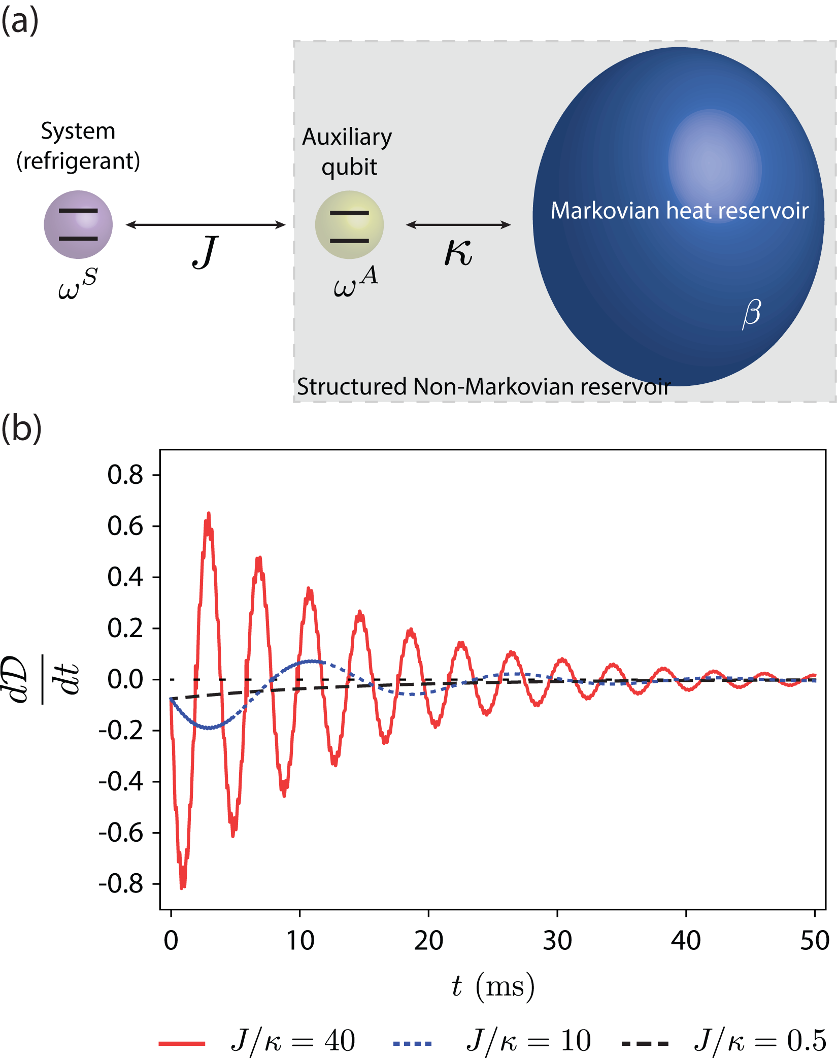
Figure 1: (a) Illustration of the structured cold heat reservoir which can induce a non-Markovian dynamics on the refrigerant of the quantum Otto refrigerator. It is composed of two parts, a Markovian heat reservoir and a two-level system (auxiliary qubit). (b)Time derivative of the trace distance between the $\left|0\right\rangle$ and $\left|1\right\rangle$ initial states for the system for different values of the ratio $J/\kappa$, 40 (red solid line), 10 (blue dotted line), and 0.5 (black dashed line) in order to indicate the non-Markovian and Markovian regimes of the model.

When the bosonic modes are in the thermal state it is possible to show that the two-qubit system $SA$ evolves under the Lindblad master equation (Raja2017, )

$$\frac{d}{dt}\rho_{t}^{SA}= -\frac{i}{\hbar}\left[H^{SA},\rho_{t}^{SA}\right]+$$

$$+\sum_{i=1,2}\gamma^{\downarrow}\left(\epsilon_{i}\right)\left(L_{i}\rho_{t}L_{i}^{\dagger}-\frac{1}{2}\left\{L_{i}^{\dagger}L_{i},\rho_{t}\right\}\right)$$

$$+\sum_{i=1,2}\gamma^{\uparrow}\left(\epsilon_{i}\right)\left(L_{i}^{\dagger}\rho_{t}L_{i}-\frac{1}{2}\left\{L_{i}L_{i}^{\dagger},\rho_{t}\right\}\right),$$ (3)

where $\gamma^{\downarrow}\left(\epsilon_{i}\right)=\frac{\pi}{2}\mathcal{J}\left(\epsilon_{i}\right)\left[1+n_{\text{BE}}\left(\epsilon_{i}\right)\right]$ and $\gamma^{\uparrow}\left(\epsilon_{i}\right)=\frac{\pi}{2}\mathcal{J}\left(\epsilon_{i}\right)n_{\text{BE}}\left(\epsilon_{i}\right)$ are the decay rates, with spectral density $\mathcal{J}\left(\omega\right)=\kappa/\pi$ and Bose-Einstein distribution $n_{\text{BE}}\left(\omega\right)=\left(e^{\beta\hbar\omega}-1\right)^{-1}$, and $L_{i}$ are the Lindblad operators (see Appendix A for more details). The quantities $\hbar\epsilon_{1}$ and $\hbar\epsilon_{2}$ are the energy gaps between different energy levels of the Hamiltonian $H^{SA}$ (see Fig. A1).

There are different notions of non-Markovian dynamics for quantum processes (Wolf2008, ; Breuer2009, ; Laine2010, ). Independent of the precise definition employed, non-Markovianity is always related to the concept of memory in the dynamics. Here, we will adopt the following notion: a system undergoes a non-Markovian dynamics if there is a flow of information from the environment to the system. In particular, we consider the trace distance as a measure of distinguishability (information) (Breuer2009, ). For two arbitrary states $\rho$ and $\sigma$, their trace distance is given by (ChuangBook, )

$$\mathcal{D}\left(\rho,\sigma\right)=\frac{1}{2}\text{Tr}\left[\sqrt{\left(\rho-\sigma\right)^{\dagger}\left(\rho-\sigma\right)}\right].$$ (4)

We denote by $\Lambda_{t,0}\left[\rho\left(0\right)\right]=\rho\left(t\right)$ the one-parameter family of dynamical maps. The dynamics is non-Markovian if $d\mathcal{D}\left(\rho_{1}\left(t\right),\rho_{2}\left(t\right)\right)/dt$ becomes positive at any time $t$ and for some pair of initial states $\rho_{1}\left(0\right)$ and $\rho_{2}\left(0\right)$ (Breuer2009, ), thus being a non-Markovian witness. Conversely, this means that, in a Markovian dynamics, the distinguishability between any pair of states always decreases monotonically in time, i.e., the derivative of the trace distance is never positive. In other words, in a non-Markovian dynamics there always exists some pair of initial states for which the distinguishability (information) increases at a given time. In particular, it is sufficient to assume a pair of initially pure and orthogonal states to witness the non-Markovianity of a qubit system (Wi=0000DFmann2012, ). For that reason, we consider such a pair of states to be the eigenstates of $\sigma_{z}$, i.e., the states $\Ket{0}$ and $\Ket{1}$, in order to determine which parameter regimes induce a non-Markovian dynamics into the refrigerant substance [see Fig. 1(b)].

We assume that the refrigerant and auxiliary qubits are resonant, $2\pi\omega^{S}=2\pi\omega^{A}=2.2\text{ kHz}$, the vacuum decay rate $\kappa=20\text{ Hz}$, and the temperature $T=2\hbar\omega^{A}/k_{\text{B}}\approx 6\text{ pK}$ for the bosonic modes. These parameters are experimentally achievable in NMR setups (Batalhao2014, ; Batalhao2015, ; Camati2016, ; Micadei2019, ). Using these parameters, in Fig. 1(b), we show for which values of the ratio $J/\kappa$ the Markovian and non-Markovian regimes are achieved. When $J/\kappa=40$ and $10$ the derivative of the trace distance becomes positive and hence the system dynamics is non-Markovian. On the other hand, for $J/\kappa=0.5$, we numerically considered 10000 pairs of initial states where one of the orthogonal states was varied throughout the north hemisphere of the Bloch sphere. We found that the derivative of the trace distance never becomes positive, hence we can suppose that the dynamics is Markovian. The plot in Fig. 1(b) shows one representative example of these curves for the mentioned pair of initial states. As shown in Ref. (Popovic2018, ), which studied a similar structured environment, the asymptotic state for the system and the auxiliary qubit is a correlated one and the reduced system state is a Gibbs state with an effective inverse temperature $\beta_{c}^{\text{eff}}$ that is different from the inverse temperature of the Markovian heat reservoir.

II.2 Quantum Otto refrigerator

Let us consider a quantum Otto refrigerator with a single-qubit refrigerant and the cycle of which is comprised by two driven adiabatic (no heat exchange) and two undriven thermalization strokes. In an Otto refrigerator with Markovian reservoirs, work and heat exchanges are associated with the adiabatic and undriven thermalization strokes, respectively. These thermodynamic quantities can be obtained through the difference between the final and initial internal energies for a given stroke. The internal energy at time $t$ is given by $U_{t}=\text{Tr}\left[\rho_{t}H\left(t\right)\right]$, where $\rho_{t}$ is the density operator of the refrigerant (system) and $H\left(t\right)$ is the Hamiltonian at a time $t$.

The refrigerant starts the cycle in the hot Gibbs state $\rho_{0}=\rho_{0}^{\text{eq,}h}=e^{-\beta_{h}H_{0}}/Z_{0}^{h}$, where $\beta_{h}=1/k_{\text{B}}T_{h}$ is the hot inverse temperature, $H_{0}$ is the initial Hamiltonian, and $Z_{0}^{h}=\text{Tr}\left[e^{-\beta_{h}H_{0}}\right]$ is the associated partition function.

In the first stroke a compression is performed on the refrigerant frequency, with driven Hamiltonian given by

$$H^{\text{com}}\left(t\right)=\frac{\hbar\omega\left(t\right)}{2}\sigma_{z},$$ (5)

where the frequency is changed as a linear ramp as $\omega\left(t\right)=\left(1-t/\tau_{1}\right)\omega_{0}+\left(t/\tau_{1}\right)\omega_{\tau_{1}}$, with $\omega_{0}$ and $\omega_{\tau_{1}}$ ($\omega_{0}>\omega_{\tau_{1}}$) being the initial and final frequency of the refrigerant, respectively. Hence the initial Hamiltonian is $H_{0}=H^{\text{com}}\left(0\right)=\left(\hbar\omega_{0}/2\right)\sigma_{z}$, where “com” stands for compression. Although this stroke is performed for a finite time, the reduced density operator of the system will not present coherence in the energy eigenbasis. This is especially due to the structure of the driving in Eq. (5) which commutes at different times, i.e., $\left[H^{\text{com}}\left(t\right),H^{\text{com}}\left(t^{\prime}\right)\right]=0$ for $t\neq t^{\prime}$. For recent studies of non-commutative driving in quantum Otto heat engines, we refer to Refs. (Camati2019, ; kosloff2019A, ). In particular, in Ref. (Camati2019, ), a quantum Otto heat engine that generates coherence in the energy basis due to the non-commutativity of the Hamiltonian was considered. It was shown that the effect of coherence in a finite-time Otto cycle induces fast oscillations in the figures of merit for the engine performance. In order to focus on the non-Markovian effects due to the engineered cold reservoir, we considered the commutative driving Hamiltonian in Eq. (5). The state at the end of the first stroke is given by $\rho_{\tau_{1}}=\mathcal{U}_{\tau_{1},0}\rho_{0}^{\text{eq,}h}\mathcal{U}_{\tau_{1},0}^{\dagger}$, where $\mathcal{U}_{t,0}=\mathcal{T}_{>}\text{exp}\left[-\left(i/\hbar\right)\int_{0}^{t}ds\,H^{\text{\text{com}}}\left(s\right)\right]$ is the time-evolution operator, $\mathcal{T}_{>}$ is the time-ordering operator, and $t\in\left[0,\tau_{1}\right]$. The final Hamiltonian is $H^{\text{com}}\left(\tau_{1}\right)=\left(\hbar\omega_{\tau_{1}}/2\right)\sigma_{z}$, such that the work performed on the refrigerant is given by $\left\langle W_{1}\right\rangle=U_{\tau_{1}}-U_{0}$.

In the second stroke the refrigerant system interacts with the engineered cold reservoir described in the previous section, the Markovian part of which has an inverse temperature $\beta_{c}=1/k_{\text{B}}T_{c}$. During this stroke, the refrigerant Hamiltonian is kept fixed at $H^{c}\left(t\right)=\left(\hbar\omega_{\tau_{1}}/2\right)\sigma_{z}$ along the time $t\in\left[\tau_{1},\tau_{2}\right]$. For further reference, we denote by $\Delta\tau_{c}=\tau_{2}-\tau_{1}$ the duration of the second stroke. Moreover, some recent developments have pointed out that incomplete (or partial) thermalization can be used to reach a better performance in quantum heat engines (Camati2019, ; Renner2019, ). For that reason we consider an incomplete thermalization, denoting by $\rho_{\tau_{2}}$ the state at the end of this stroke. Furthermore, the structure of the engineered cold reservoir will be set to generate a Markovian or non-Markovian dynamics on the refrigerant substance. This choice is adjusted depending on the ratio of the coupling constant $J$ between the refrigerant and the auxiliary qubit and the internal coupling $\kappa$ between the auxiliary qubit and the cold Markovian reservoir as considered in Fig. 1(b). Since $\kappa$ should be small (weak coupling) the regimes are essentially obtained by varying $J$. The heat absorbed by the quantum refrigerant is given by $\left\langle Q_{c}\right\rangle=U_{\tau_{2}}-U_{\tau_{1}}$.

In the third stroke, the refrigerant is decoupled from the structured cold reservoir and its frequency is increased from $\omega_{\tau_{1}}$ to $\omega_{0}$ by means of an adiabatic expansion. The driving Hamiltonian for this stroke is $H^{\text{exp}}\left(t\right)=H^{\text{com}}\left(\tau_{1}+\tau_{2}-t\right)$ applied for the time interval $t\in\left[\tau_{2},\tau_{3}\right]$, where “exp” stands for expansion. The final state is $\rho_{\tau_{3}}=\mathcal{V}_{\tau_{3},\tau_{2}}\rho_{2}\mathcal{V}_{\tau_{3},\tau_{2}}^{\dagger}$ where $\mathcal{V}_{\tau_{3},\tau_{2}}=\mathcal{T}_{>}\text{exp}\left[-\left(i/\hbar\right)\int_{\tau_{2}}^{\tau_{3}}dt\>H^{\text{exp}}\left(t\right)\right]$ is the evolution operator associated to the adiabatic expansion. The time duration of the third stroke is assumed to be the same as for the first stroke, i.e., $\tau_{3}-\tau_{2}=\tau_{1}$, so that $H^{\text{exp}}\left(\tau_{3}\right)=H^{\text{com}}\left(0\right)$. The work performed on the refrigerant during this stroke is $\left\langle W_{3}\right\rangle=U_{\tau_{3}}-U_{\tau_{2}}$. At this point we can define the total work performed on the refrigerant as $\left\langle W_{\text{net}}\right\rangle=\left\langle W_{1}\right\rangle+\left\langle W_{3}\right\rangle$.

Finally, in the fourth stroke and in order to close the cycle, this last stroke comprises a complete thermalization of the refrigerant with the hot reservoir at inverse temperature $\beta_{h}$. During this process the Hamiltonian is kept fixed at $H^{\text{exp}}\left(\tau_{3}\right)=\left(\hbar\omega_{0}/2\right)\sigma_{z}$ along the time $t\in\left[\tau_{3},\tau_{4}\right]$. Once the condition $\tau_{4}-\tau_{3}\gg\tau_{\text{rel}}^{h}$ is fulfilled, where $\tau_{\text{rel}}^{h}$ is the relaxation time for the hot Markovian heat reservoir, the final state reaches $\rho_{\tau_{4}}=\rho_{0}^{\text{eq,}h}$. The heat absorbed by the refrigerant is given by $\left\langle Q_{h}\right\rangle=U_{\tau_{4}}-U_{\tau_{3}}$. The total time duration of a single cycle will be given by $\tau_{\text{cycle}}=\tau_{4}=\tau_{1}+\Delta\tau_{c}+\tau_{1}+\Delta\tau_{h}$.

Before we move forward to the discussion of the performance, we define some other quantities that will turn out to be relevant. In the second stroke, the first law of thermodynamics implies that $\left\langle Q_{c}^{S}\right\rangle+\left\langle Q_{c}^{R}\right\rangle+\Delta V_{c}^{SR}=0$, where $-\left\langle Q_{c}^{R}\right\rangle$ is the energy released by the engineered cold reservoir $R$, and $\Delta V_{c}^{SR}$ is the change in the interaction energy between $S$ and $R$. The total energy released by the engineered cold reservoir is, therefore, given by the expression

$$-\left\langle Q_{c}^{R}\right\rangle=\left\langle Q_{c}^{S}\right\rangle+\Delta V_{c}^{SR}.$$ (6)

For our model, the auxiliary qubit couples weakly to the Markovian heat reservoir, hence we have $\Delta V_{c}^{SR}=\Delta V_{c}^{SA}$, where $\Delta V_{c}^{SA}=\text{Tr}\left[\rho_{\tau_{2}}^{SA}H_{\text{int}}^{SA}\right]-\text{Tr}\left[\rho_{\tau_{1}}^{SA}H_{\text{int}}^{SA}\right]$ is the interaction energy of the $SA$ composite system during the second stroke.

III Performance of the quantum Otto refrigerator

The purpose of a refrigerator is to cool down the cold reservoir, hence the quantity that has to fundamentally be considered to assess the performance of a refrigerator is $-\left\langle Q_{c}^{R}\right\rangle$, i.e., the energy released by the cold reservoir. Therefore, the COP is defined by

$$\epsilon=\frac{-\left\langle Q_{c}^{R}\right\rangle}{\left\langle W_{\text{net}}^{S}\right\rangle}=\frac{\left\langle Q_{c}^{S}\right\rangle+\Delta V_{c}^{SR}}{\left\langle W_{\text{net}}^{S}\right\rangle},$$ (7)

where we used Eq. (6) to write the last equality. Similarly, the cooling power will be given by $\left\langle\Gamma\right\rangle=-\left\langle Q_{c}^{R}\right\rangle/\tau_{\text{cycle}}$ while the injected power is $\left\langle\mathcal{P}\right\rangle=\left\langle W_{\text{net}}^{S}\right\rangle/\tau_{\text{cycle}}$. When the interaction energy is small compared to the heat absorbed by the system, i.e., $\left\langle Q_{c}^{S}\right\rangle+\Delta V_{c}^{SR}\approx\left\langle Q_{c}^{S}\right\rangle$, we can see that the usual expressions for the figures of merit of a refrigerator are recovered. One such a situation happens in classical thermodynamics, where the coupling between the refrigerant and the reservoir is small (weak-coupling regime). Not only that, the refrigerant is a macroscopic system (a fluid or a gas) so that the internal energy, which scales with the volume, is larger than the interaction energy, which scales with the area (boundary). On the other hand, if the refrigerant is strongly coupled to the reservoir, the interaction energy starts playing a role in the thermodynamics (Newman2017, ; Newman2019, ) and in the performance analysis of the refrigerator.

We obtain the following analytical expressions for any quantum refrigerant (and not only for a qubit), as described in Appendix B. We later restrict to our specific model again to present our numerical analysis. The COP defined in Eq. (8) can be written as

$$\epsilon=\gamma\frac{\epsilon_{\text{Carnot}}}{1+\epsilon_{\text{Carnot}}\mathcal{L}},$$ (8)

where $\epsilon_{\text{Carnot}}=\left(\beta_{c}/\beta_{h}-1\right)^{-1}$ is the Carnot COP and

$$\mathcal{L}=\frac{D\left(\rho_{\tau_{1}}||\rho_{\tau_{1}}^{\text{eq,}c}\right)-D\left(\rho_{\tau_{2}}||\rho_{\tau_{2}}^{\text{eq,}c}\right)+D\left(\rho_{\tau_{3}}||\rho_{\tau_{3}}^{\text{eq,}h}\right)}{\beta_{h}\langle Q_{c}\rangle}$$ (9)

is the COP lag, previously defined for quantum engines (Camati2019, ; Peterson2018, ; Campisi2016, ). The multiplicative term in Eq. (8) is given by

$$\gamma=\left(1+\frac{\Delta V_{c}^{SR}}{\left\langle Q_{c}^{S}\right\rangle}\right),$$ (10)

and we call it the interaction-energy parameter. Similarly, the cooling power can be written as

$$\left\langle\Gamma\right\rangle=\gamma\frac{\left\langle Q_{c}^{S}\right\rangle}{\tau_{\text{cycle}}}.$$ (11)

From these two equations we can see that the parameter $\gamma$ quantifies how the COP and the cooling power change in the presence of a non-negligible interaction energy between the refrigerant and the engineered cold reservoir.

In order to remain in the operation regime of a refrigerator, the thermodynamic quantities must satisfy the constraints $-\left\langle Q_{c}^{R}\right\rangle>0$, $\left\langle W_{\text{net}}\right\rangle>0$, and $\left\langle Q_{h}^{R}\right\rangle<0$. These constraints imply that the interaction-energy parameter must be positive, i.e., $\gamma>0$ (see Appendix B). For our specific refrigerator cycle, the COP can be also written as $\epsilon=\gamma\epsilon_{\text{Otto}}$, where $\epsilon^{\text{Otto}}=\omega_{\tau_{1}}/\left(\omega_{0}-\omega_{\tau_{1}}\right)$ (see Appendix C). Therefore, the interaction-energy parameter should be upper bounded by $1$ so that the COP is smaller than the Otto COP. For a wide range of parameters, we verified numerically that our refrigerator does not surpass the Otto COP. If one assess the performance of the refrigerator ignoring this parameter $\gamma$, either by simply not accounting for it or because one might not be aware if the interaction energy is not negligible, the performance of the refrigerator will be overestimated by precisely $1/\gamma$. More specifically, ignoring a parameter of $\gamma=0.9$, the COP and the cooling power would be overestimated by about $11\%$, meaning that the computed COP and cooling power will be $11\%$ larger than the true COP and cooling power.

Before we present our numerical analysis, we note that we have chosen a driving Hamiltonian that commutes at different times, $\left[H^{\text{com}}\left(t\right),H^{\text{com}}\left(t^{\prime}\right)\right]=0$. This implies an Otto cycle without quantum friction (Feldmann2006, ; Camati2019, ; Batalhao2015, ; Feldmann01, ; Feldman02, ; Campo01, ; Thomas01, ; Plastina01, ; Paternostro2014, ). We assume this dynamics for the driving Hamiltonian in order to solely focus on the non-Markovian aspects of the Otto cycle. Since our refrigerator has no quantum friction, in the Markovian regime where the interaction energy is negligible, $\gamma=1$, the refrigerator reaches the Otto COP, $\epsilon=\epsilon_{\text{Otto}}$. In the case of the non-Markovian regime, even in the absence of quantum friction, the Otto COP will not be generally reached, due to the presence of the interaction energy.

In the following, we performed a numerical simulation of our quantum Otto refrigerator, assuming energy scales compatible with quantum thermodynamics experiments performed in NMR setups (Peterson2018, ; Batalhao2014, ; Batalhao2015, ; Camati2016, ; Micadei2019, ). The initial and final gaps of the compression stroke are chosen as $\omega_{0}/2\pi=3.6\text{ kHz}$ and $\omega_{\tau_{1}}/2\pi=2.2\text{ kHz}$, respectively. The cold ($T_{c}$) and hot ($T_{h}$) temperatures are chosen such that $T_{c}=1/\left(2.5\omega_{\tau_{1}}\right)$ and $T_{h}=1/\left(2.5\omega_{0}\right)$ with inverse temperatures given by $\beta_{c}=1/T_{c}$ and $\beta_{h}=1/T_{h}$. Finally, we assume that the vacuum decay rates of the cold and hot Markovian reservoirs are $\gamma_{c}=\gamma_{h}=20\text{ Hz}$, where $\gamma_{c}=\kappa$ from Sec. II.1.

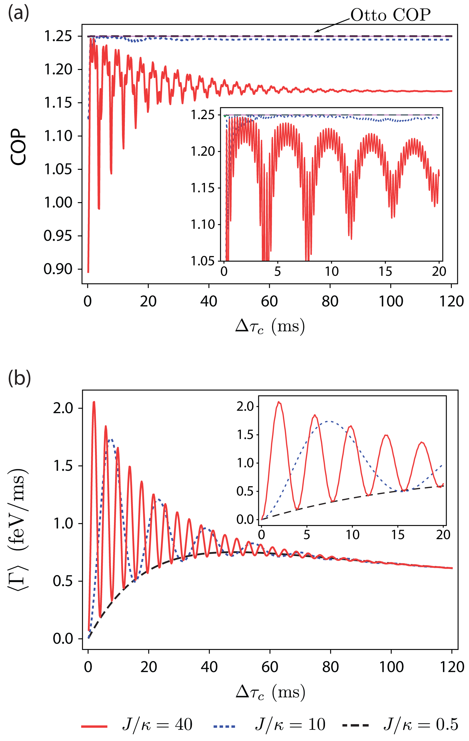
Figure 2: COP (a) and cooling power (b) as a function of the time of the second stroke $\Delta\tau_{c}$ for three values of the ratio $J/\kappa$: 40 (solid red line), 10 (dotted blue line), and 0.5 (dashed black line). The oscillations of the COP are very fast, as seen in the inset of (a), and hence the oscillations seen in (a) represent just a coarse graining of the actual oscillations. From both figures we can see that the larger the ratio $J/\kappa$ is, which implies a larger effect of the non-Markovian dynamics, the larger the effect on the performance as well, namely, larger oscillation amplitudes and frequency of oscillations. For the Markovian regime ($J/\kappa=0.5$), there is no oscillation in the cooling power, and the COP is the Otto COP, as expected from the fact that our cycle has no quantum friction. We considered $\tau_{1}=0.75\text{ ms}$.

We see in Fig. 2 that the Markovian regime (dashed black line) reproduces the expected results. The COP reaches the Otto limit, since there is no quantum friction in our cycle. Furthermore, the cooling power $\langle\Gamma\rangle$ decreases for second strokes of long duration, for both the non-Markovian and the Markovian regimes. We can clearly see the effect of the non-Markovian dynamics on both the COP and the cooling power, which is to induce oscillations of different amplitudes and frequencies, depending on the ratio $J/\kappa$. For a larger ratio of $J/\kappa$ [solid red line in Fig. 2(b)] the cooling power oscillates quite more frequently but does not have a maximum value that exceeds considerably the maximum of a moderate ratio of $J/\kappa$ [dotted blue line in Fig. 2(b)]. In the non-Markovian regime, the oscillation frequency increases considerably meaning that a better control of the allocation time on the second stroke is needed to end up in the peak of the cooling power curves. On the other hand, in Fig. 2(a), a larger ratio of $J/\kappa$ (solid red line) degrades considerably the COP and the timescale for the oscillations are much smaller than for the cooling power [compare the insets in Figs. 2(a) and 2(b)]. This means that, for larger values of $J/\kappa$ an extremely good amount of control should be necessary to make the refrigerator operate in the maximum of the corresponding COP. We also see that, for a moderate ratio of $J/\kappa$ (dotted blue line), although the COP is smaller than the Otto COP it remains very close to it throughout the time range considered in the plot. In other words, the value of the COP for moderate values of $J/\kappa$ does not change much from its asymptotic value (reached for long time durations of the second stroke $\Delta\tau_{c}$). Therefore, for our model of an engineered cold reservoir, we can conclude that a moderate non-Markovian dynamics ($J/\kappa=10$) performs generally better than a Markovian ($J/\kappa=0.5$) or a strong non-Markovian ($J/\kappa=40$) regime. Comparing to the Markovian regime, the moderate non-Markovian regime has almost the same COP and improves considerably on the cooling power, whereas, comparing the moderate (dotted blue line) with the strong (solid red line) non-Markovian regime, the COP is larger while the cooling power oscillates with a smaller frequency, making it easier to adjust the cycle time to operate in the optimal regimes.

We now fix three values for the duration of the second stroke $\Delta\tau_{c}$ and analyze how the performance of the refrigerator changes with the ratio $J/\kappa$ (see Fig. 3). For a long second stroke, $\Delta\tau_{c}=120\text{ ms}$ (dashed black line), the refrigerator and auxiliary qubits practically reach their asymptotic states. We see that the COP degrades very quickly with increasing $J/\kappa$, and that in the Markovian regime ($J/\kappa\apprle 0.5$) it reaches the Otto COP [see dashed black line in Fig. 3(a)]. The cooling power, on the other hand, stays constant, showing that in the asymptotic regime the non-Markovian regime is no better or worse than the Markovian regime [see dashed black line in Fig. 3(b)]. For a moderate duration of the second stroke, the COP still decreases quickly but with an oscillating profile, whereas the cooling power also does not represent a big difference between the non-Markovian and Markovian regimes [see solid red lines in Figs. 3(a) and 3(b)]. As expected, for a very short duration of the second stroke [see dotted blue lines in Figs. 3(a) and 3(b)] and for the Markovian regimes, the COP is the Otto limit and the cooling power is close to zero, since the refrigerant has not much time to absorb the energy from the cold reservoir. When the ratio $J/\kappa$ starts to get larger, the non-Markovian dynamics starts to impact more strongly. The cooling power starts increasing and then oscillates. It is interesting to note that, even though the COP is strictly smaller than the Otto COP for the non-Markovian regime, it stays very close to the Otto COP for a reasonable portion of the initial values of $J/\kappa$. Then, there is a brief decay in the COP which starts increasing again and stays almost constant before decreasing abruptly. This behavior is notably different than for a moderate duration of the second stroke. We highlighted in gray the range of the $J/\kappa$ parameter for which the cooling power is close to its maximum. For these shaded regions (in Figs. 3(a) and 3(b)), the COP is about 99.8% and about 97.2% of the Otto limit, for the first and second highlighted region from left to right, respectively. These regions point out the most interesting parameter regimes in which the refrigerator should be operated, among the three plotted curves. Figures 3(a) and 3(b) show also how the short duration of the second stroke makes a huge difference in the performance of the non-Markovian refrigerator.

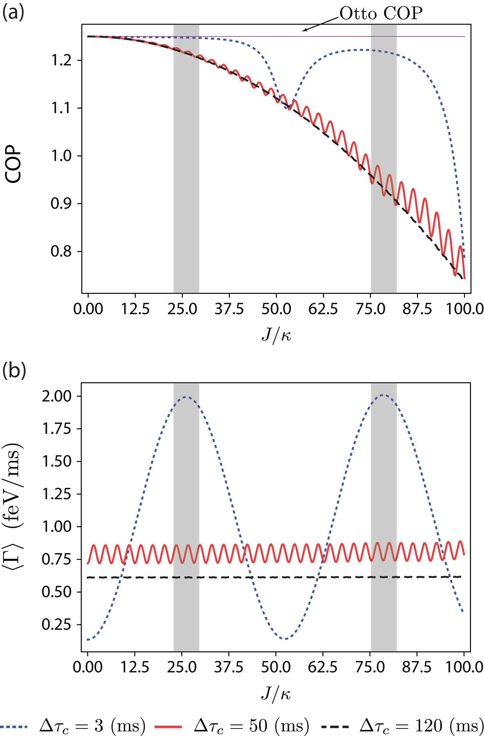
Figure 3: COP (a) and cooling power (b) as a function of the ratio $J/\kappa$ for three values of the duration of the second stroke $\Delta\tau_{c}$: 3 ms (dotted blue line), 50 ms (solid red line), and 120 ms (dashed black line). The Markovian regime corresponds to values of about or smaller than $J/\kappa=0.5$. The gray area on both figures shows the region of $J/\kappa$ values for which the cooling power is close to its maximum. We considered $\tau_{1}=0.75\text{ ms}$.

We finish our discussion in this section by showing how the mutual information between the refrigerant and the auxiliary qubit changes in the second stroke (see Fig. 4). The mutual information is given by $I_{\tau_{2}}^{S:A}=S\left(\rho_{\tau_{2}}^{S}\right)+S\left(\rho_{\tau_{2}}^{A}\right)-S\left(\rho_{\tau_{2}}^{SA}\right)$, where $\rho_{\tau_{2}}^{SA}$, $\rho_{\tau_{2}}^{S}$, and $\rho_{\tau_{2}}^{A}$ are the composite $SA$, the refrigerant $S$, and the auxiliary qubit $A$ states at the end of the second stroke. The quantity $S\left(\rho\right)=-\text{Tr}\left[\rho\ln\rho\right]$ is the von Neumann entropy. We see that, for $J/\kappa=40$ (solid red line), the mutual information oscillates very rapidly, reaching a finite value at the end, showing that the asymptotic $SA$ state is correlated (Newman2017, ). For a moderate non-Markovian dynamics, $J/\kappa=10$ (dotted blue line), the mutual information also oscillates, but with a smaller frequency, reaching almost zero at the end. For the Markovian regime, $J/\kappa=0.5$ (dashed black line), the mutual information is almost zero everywhere. Comparing the oscillations in the inset of Fig. 4 and those of the inset of Fig. 2(b), we see that the peaks of the cooling power are not associated directly to the peaks of the mutual information. The same conclusion applies comparing the mutual information with the inset of Fig. 2(a). This shows that, although the presence of mutual information is important because it is related to the non-Markovian dynamics, the improvement of the refrigerator performance is not directly related to the correlation created between the refrigerant and the engineered cold reservoir.

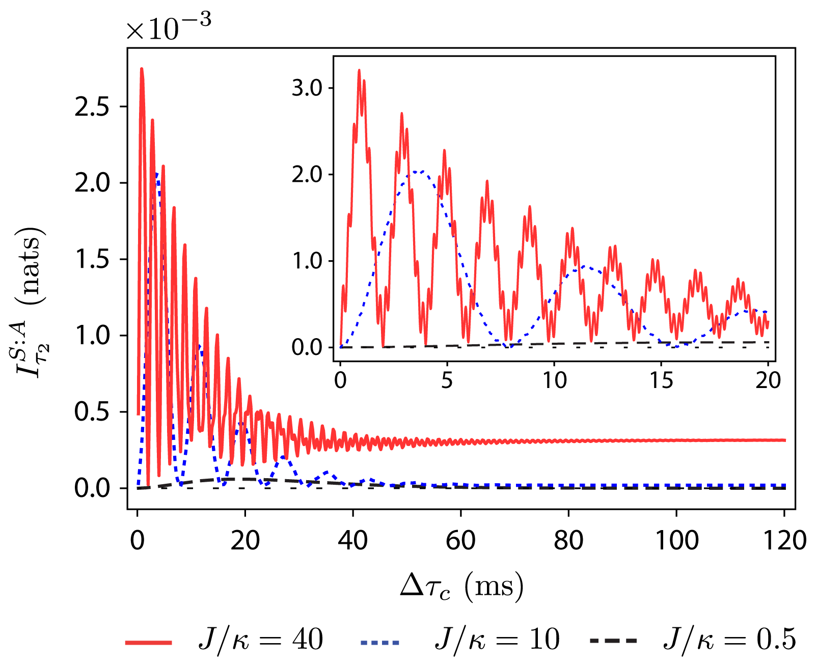
Figure 4: Mutual information $I_{\tau_{2}}^{S:A}$ between the refrigerant and the auxiliary qubit at the end of the second stroke. For the strong non-Markovian regime, the solid red line with $J/\kappa=40$, the mutual information oscillates very rapidly (see the inset). The oscillatory behavior of the plot is a coarse graining of the true oscillations. We can see that in the asymptotic regime, for a long duration of the second stroke, the $SA$ system reaches a correlated state with given mutual information. In the Markovian regime the correlations are zero (dashed black line) while for a moderate non-Markovian regime (dotted blue line) it oscillates less frequently and almost reaches zero at the end. We considered $\tau_{1}=0.75\text{ ms}$ and $1\text{ nat }=1/\ln 2\approx 1.44\text{ bit}$.

IV Conclusions

We analyzed the performance of a quantum Otto refrigerator the refrigerant of which interacts with an engineered cold reservoir, comprised by a Markovian reservoir and an auxiliary two-level system. Depending on the coupling between the refrigerant and the structured cold environment the dynamics of the refrigerant can be either Markovian or non-Markovian, changing the performance of the refrigerator. In our model, the non-Markovian regime is reached when the interaction between the refrigerant and the reservoir is strong, in the sense that the contribution of the interaction energy between the refrigerant and the engineered reservoir cannot be neglected. Concisely, the heat removed from the cold reservoir (the prime purpose of a refrigerator) is not the heat absorbed by the refrigerant, because the interaction Hamiltonian stores a nontrivial amount of energy.

Taking the interaction energy into account, we defined the figures of merit for the refrigerator: the COP, the cooling power, and the injected power. We showed that the interaction-energy contribution can be recast as a parameter $\gamma$, given by Eq. (10), multiplying the usual expressions for the COP and cooling power, which disregard such a contribution. These analytical expressions are valid irrespective of the nature of the quantum refrigerant. In light of these expressions, we can conclude that an overestimation of the refrigerator performance would be made if such an interaction-energy contribution was ignored in the analysis. In fact, it is in principle possible to find an operation regime in which one might think the refrigerator is working properly, because the refrigerant is absorbing energy, but in fact it is not operating as a refrigerator at all, i.e., there is no energy being removed from the cold reservoir. The increase in the refrigerant energy comes solely from the interaction energy.

Performing a numerical analysis, we observed the expected behavior for the Markovian regime of operation, reached for a sufficiently small coupling between the refrigerant and the engineered cold reservoir. On the other hand, for the non-Markovian regimes of operation, we see that both the COP and the cooling power start oscillating, a feature coming from the backflow of information from the non-Markovian environment. Both COP and cooling power oscillate faster as the coupling and the non-Markovian effect increase, but the COP decreases significantly as well, while the cooling power increases slightly for a small time of interaction between them (duration of the second stroke). We conclude that, at least for the model considered in our paper, a moderate non-Markovian effect improves the performance of the refrigerator, if compared to the Markovian or strong non-Markovian regimes. We also point out that in order to exploit the non-Markovian effects it is important to operate the refrigerator in a sufficiently short interaction timescale between the refrigerant and the engineered cold reservoir.

The finite-time performance of the present quantum Otto refrigerator may be enhanced by the information backflow provided one has sufficient control over the time allocated in each stroke. The parameters considered in the numerical simulation can be experimentally realized with current technologies, for instance, in nuclear magnetic resonance setups. Along with other studies addressing non-Markovian effects in quantum thermodynamics, we hope that our analyses help to unveil the role of memory effects in quantum thermal machines.

Appendix A Master Equation of the Non-Markovian Model

The master equation of the non-Markovian model employed is given by Eq. (3). Here, we provide some details on the derivation of this master equation. We will follow the approach of Refs. (Rivas2010, ; Rivas2012book, ).

We begin considering the diagonalization of the two-qubit Hamiltonian [Eq. (2)]

$$H^{SA}=\sum_{i=S,A}\frac{\hbar\omega^{i}}{2}\sigma_{z}^{i}+\hbar J\sigma_{x}^{S}\sigma_{x}^{A}.$$ (A1)

The eigenvectors and eigenvalues are:

$$\Ket{E_{3}}=\alpha\Ket{00}+\xi\Ket{11}\text{ and }E_{3}=\frac{\hbar}{2}\sqrt{4J^{2}+\Omega^{2}};$$ (A2)

$$\Ket{E_{2}}=\eta\Ket{01}-\delta\Ket{10}\text{ and }E_{2}=\frac{\hbar}{2}\sqrt{4J^{2}+\Delta^{2}};$$ (A3)

$$\Ket{E_{1}}=\delta\Ket{01}+\eta\Ket{10}\text{ and }E_{1}=-E_{2};$$ (A4)

$$\Ket{E_{0}}=-\xi\Ket{00}+\alpha\Ket{11}\text{ and }E_{0}=-E_{3}.$$ (A5)

We introduced the parameters $\Delta=\omega^{S}-\omega^{A}$, $\Omega=\omega^{S}+\omega^{A}$,

$$\alpha=\frac{\Omega+\sqrt{4J^{2}+\Omega^{2}}}{\sqrt{4J^{2}+\left(\Omega+\sqrt{4J^{2}+\Omega^{2}}\right)^{2}}},$$ (A6)

$$\xi=\frac{2J}{\sqrt{4J^{2}+\left(\Omega+\sqrt{4J^{2}+\Omega^{2}}\right)^{2}}},$$ (A7)

$$\eta=\frac{\Delta+\sqrt{4J^{2}+\Delta^{2}}}{\sqrt{4J^{2}+\left(\Delta+\sqrt{4J^{2}+\Delta^{2}}\right)^{2}}},$$ (A8)

and

$$\delta=\frac{-2J}{\sqrt{4J^{2}+\left(\Delta+\sqrt{4J^{2}+\Delta^{2}}\right)^{2}}}.$$ (A9)

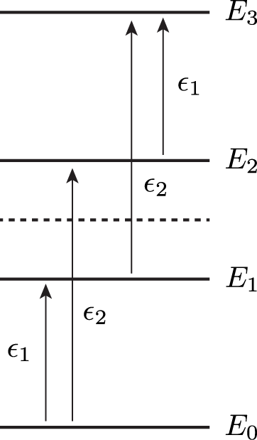
Figure A1: Transition frequencies. Among the six positive frequencies (from a low- to a high-energy level) only four appear on the master equation due to the structure of the interaction Hamiltonian. These are shown in the energy diagram.

The master equation of the two-qubit system is given by (Rivas2012book, ; Breuer2002book, ; Alicki2007book, )

$$\frac{d}{dt}\rho_{t}^{SA}=-\frac{i}{\hbar}\left[H^{SA},\rho_{t}^{SA}\right]+\mathcal{D}\left(\rho_{t}^{SA}\right),$$ (A10)

where

$$\mathcal{D}\left(\rho_{t}^{SA}\right)= \sum_{\omega\in\mathcal{F}}\sum_{k,l=1,2}\gamma_{kl}\left(\omega\right)$$

$$\times\left[A_{l}\left(\omega\right)\rho_{t}^{SA}A_{k}^{\dagger}\left(\omega\right)-\frac{1}{2}\left\{A_{k}^{\dagger}\left(\omega\right)A_{l}\left(\omega\right),\rho_{t}^{SA}\right\}\right]$$ (A11)

is the dissipator superoperator. We note that we have disregarded the Lamb-shift Hamiltonian since it contributes to an overall energy shift. The set $\mathcal{F}$ is comprised by all, positive and negative, transition frequencies $\omega_{nm}=\left(E_{m}-E_{n}\right)/\hbar$ for $m,n\in\left\{0,1,2,3\right\}$. Since the composite system $SA$ is a four-level system, there are 12 transition frequencies, 6 positive and 6 negative, $\omega_{nm}$ and $\omega_{mn}=-\omega_{nm}$ with $n<m$, respectively. As we will explain below, among the 6 positive (or negative) transition frequencies only 2 doubly-degenerate ones are relevant to our problem (see Fig. A1). The positive transition frequencies are $\omega_{01}=\omega_{23}=\epsilon_{1}$ and $\omega_{02}=\omega_{13}=\epsilon_{2}$, where

$$\epsilon_{1}=\frac{1}{2}\left[\sqrt{\Omega^{2}+4J^{2}}-\sqrt{\Delta^{2}+4J^{2}}\right]$$ (A12)

and

$$\epsilon_{2}=\frac{1}{2}\left[\sqrt{\Omega^{2}+4J^{2}}+\sqrt{\Delta^{2}+4J^{2}}\right].$$ (A13)

Before we proceed, we rewrite the interaction Hamiltonian [Eq. (1)] of the two-qubits system and the heat reservoir as

$$V^{AR}= \int_{0}^{\omega_{\text{max}}}d\omega\,h\left(\omega\right)\left(\sigma_{+}^{A}\otimes b_{\omega}+\sigma_{-}^{A}\otimes b_{\omega}^{\dagger}\right)$$

$$= A_{1}\otimes B_{1}+A_{2}\otimes B_{2},$$ (A14)

where $\sigma_{\pm}=\left(\sigma_{x}\pm i\sigma_{y}\right)/2$ and the continuum limit has been taken at the Hamiltonian level (Rivas2012book, ). The defined operators are: $A_{1}=\sigma_{x}^{A}$, $A_{2}=\sigma_{y}^{A}$, $B_{1}=\int_{0}^{\omega_{\text{max}}}d\omega\,h\left(\omega\right)\frac{b_{\omega}^{\dagger}+b_{\omega}}{2}$, and $B_{2}=\int_{0}^{\omega_{\text{max}}}d\omega\,h\left(\omega\right)\frac{ib_{\omega}-ib_{\omega}^{\dagger}}{2}$. Using the relation $B_{i}=\int_{-\omega_{\text{max}}}^{\omega_{\text{max}}}d\omega\,B_{i}\left(\omega\right)$, one can obtain the operators $B_{1}\left(\omega\right)=\frac{h\left(\omega\right)b_{\omega}}{2}$, $B_{1}\left(-\omega\right)=\frac{h\left(\omega\right)b_{\omega}^{\dagger}}{2}$, $B_{2}\left(\omega\right)=i\frac{h\left(\omega\right)b_{\omega}}{2}$, and $B_{2}\left(-\omega\right)=-i\frac{h\left(\omega\right)b_{\omega}^{\dagger}}{2}$. Since there are two reservoirs operators, $k,l\in\left\{1,2\right\}$ in Eq. (A11) and, therefore, there are four decay rates for each transition frequency $\omega\in\mathcal{F}$.

First, we find the decay rates for a given $\omega$, which are given by the formula (Rivas2012book, )

$$\gamma_{kl}\left(\omega\right)= \int_{-\infty}^{+\infty}ds\,e^{i\omega s}\text{Tr}_{R}\left[B_{k}\left(s\right)B_{l}\rho^{R,\text{eq}}\right]$$

$$= 2\pi\text{Tr}_{R}\left[B_{k}\left(\omega\right)B_{l}\rho^{R,\text{eq}}\right],$$ (A15)

where $\omega\in\mathcal{F}$ and $\rho^{R,\text{eq}}$ is the Gibbs state of the reservoir. Knowing that $\text{Tr}_{R}\left[a_{\omega}a_{\omega^{\prime}}^{\dagger}\rho^{R,\text{eq}}\right]=\left[1+n_{\text{BE}}\left(\omega\right)\right]\delta\left(\omega-\omega^{\prime}\right)$, $\text{Tr}_{R}\left[a_{\omega}^{\dagger}a_{\omega^{\prime}}\rho^{R,\text{eq}}\right]=n_{\text{BE}}\left(\omega\right)\delta\left(\omega-\omega^{\prime}\right)$, and $\text{Tr}_{R}\left[a_{\omega}a_{\omega^{\prime}}\rho^{R,\text{eq}}\right]=\text{Tr}_{R}\left[a_{\omega}^{\dagger}a_{\omega^{\prime}}^{\dagger}\rho^{R,\text{eq}}\right]=0$, one can show for the positive transition frequencies $\omega\in\mathcal{F}_{+}=\left\{\omega\in\mathcal{F}\,|\,\omega\geq 0\right\}$ that

$$\gamma_{11}\left(\omega\right)=\frac{\pi}{2}J\left(\omega\right)\left[1+n_{\text{BE}}\left(\omega\right)\right],$$ (A16)

$$\gamma_{12}\left(\omega\right)=-i\frac{\pi}{2}J\left(\omega\right)\left[1+n_{\text{BE}}\left(\omega\right)\right],$$ (A17)

$$\gamma_{21}\left(\omega\right)=i\frac{\pi}{2}J\left(\omega\right)\left[1+n_{\text{BE}}\left(\omega\right)\right],$$ (A18)

and

$$\gamma_{22}\left(\omega\right)=\frac{\pi}{2}J\left(\omega\right)\left[1+n_{\text{BE}}\left(\omega\right)\right],$$ (A19)

where $n_{\text{BE}}\left(\omega\right)=\left(e^{\beta\hbar\omega}-1\right)^{-1}$ is the Bose-Einstein distribution and $J\left(\omega\right)=\left[h\left(\omega\right)\right]^{2}$ is the spectral density. On the other hand, for the negative transition frequencies $\omega\in\mathcal{F}_{-}=\left\{\omega\in\mathcal{F}\,|\,\omega<0\right\}$, one finds

$$\gamma_{11}\left(-\omega\right)=\frac{\pi}{2}J\left(\omega\right)n_{\text{BE}}\left(\omega\right),$$ (A20)

$$\gamma_{12}\left(-\omega\right)=i\frac{\pi}{2}J\left(\omega\right)n_{\text{BE}}\left(\omega\right),$$ (A21)

$$\gamma_{21}\left(-\omega\right)=-i\frac{\pi}{2}J\left(\omega\right)n_{\text{BE}}\left(\omega\right),$$ (A22)

and

$$\gamma_{22}\left(-\omega\right)=\frac{\pi}{2}J\left(\omega\right)n_{\text{BE}}\left(\omega\right).$$ (A23)

Now, we need the operators $A_{k}\left(\omega\right)$, which come from the system operators $\sigma_{x}^{A}$ and $\sigma_{y}^{A}$. They are given by (Rivas2012book, ; Breuer2002book, )

$$A_{k}\left(\omega_{nm}\right)=\sum_{E_{m}-E_{n}=\omega_{nm}}\Pi_{n}A_{k}\Pi_{m},$$ (A24)

where the projection operators are $\Pi_{n}=\Ket{E_{n}}\Bra{E_{n}}$. Since $A_{1}=\mathds{1}^{S}\otimes\sigma_{x}^{A}$ and $A_{2}=\mathds{1}^{S}\otimes\sigma_{y}^{A}$ one can show that

$$\Pi_{n}A_{1}\Pi_{m}=\begin{pmatrix}0&\alpha\eta-\delta\xi&-\left(\alpha\delta+\eta\xi\right)&0\\ \alpha\eta-\delta\xi&0&0&\alpha\delta+\eta\xi\\ -\left(\alpha\delta+\eta\xi\right)&0&0&\alpha\eta-\delta\xi\\ 0&\alpha\delta+\eta\xi&\alpha\eta-\delta\xi&0\end{pmatrix}$$ (A25)

and

$$\Pi_{n}A_{2}\Pi_{m}=\begin{pmatrix}0&i\left(\alpha\eta+\delta\xi\right)&-i\left(\alpha\delta-\eta\xi\right)&0\\ -i\left(\alpha\eta+\delta\xi\right)&0&0&i\left(\alpha\delta-\eta\xi\right)\\ i\left(\alpha\delta-\eta\xi\right)&0&0&i\left(\alpha\eta+\delta\xi\right)\\ 0&-i\left(\alpha\delta-\eta\xi\right)&-i\left(\alpha\eta+\delta\xi\right)&0\end{pmatrix}.$$ (A26)

Note how the operators $A_{k}\left(\omega\right)$ associated with the transition frequencies $\omega_{03}$, $\omega_{30}$, $\omega_{12}$, $\omega_{21}$ are identically zero. That is why these transition frequencies are not relevant, i.e., because their associated operators are zero due to the structure of the interaction Hamiltonian. Explicitly, one has

$$A_{k}\left(\epsilon_{1}\right)=\Pi_{0}A_{k}\Pi_{1}+\Pi_{2}A_{k}\Pi_{3},$$ (A27)

$$A_{k}\left(\epsilon_{2}\right)=\Pi_{0}A_{k}\Pi_{2}+\Pi_{1}A_{k}\Pi_{3},$$ (A28)

$A_{k}\left(-\epsilon_{1}\right)=A_{k}^{\dagger}\left(\epsilon_{1}\right)$, and $A_{k}\left(-\epsilon_{2}\right)=A_{k}^{\dagger}\left(\epsilon_{2}\right)$, for $k\in\left\{1,2\right\}$. In summary, there are four system operators, two for each nondegenerate transition frequency $\epsilon_{1}$ and $\epsilon_{2}$. This means that there will be four dissipative channels in the master equation [see Eq. (3)]. Replacing the decay rates $\gamma_{kl}\left(\omega\right)$ and system operators $A_{k}\left(\omega\right)$, one obtains the master equation employed, whose dissipator is given by

$${\normalcolor\mathcal{D}\left(\rho_{t}^{SA}\right)=} {\normalcolor\gamma^{\downarrow}\left(\epsilon_{1}\right)\left[L_{1}\left(\epsilon_{1}\right)\rho_{t}^{SA}L_{1}^{\dagger}\left(\epsilon_{1}\right)-\frac{1}{2}\left\{L_{1}^{\dagger}\left(\epsilon_{1}\right)L_{1}\left(\epsilon_{1}\right),\rho_{t}^{SA}\right\}\right]}$$

$${\normalcolor+\gamma^{\downarrow}\left(\epsilon_{2}\right)\left[L_{2}\left(\epsilon_{2}\right)\rho_{t}^{SA}L_{2}^{\dagger}\left(\epsilon_{2}\right)-\frac{1}{2}\left\{L_{2}^{\dagger}\left(\epsilon_{2}\right)L_{2}\left(\epsilon_{2}\right),\rho_{t}^{SA}\right\}\right]}$$

$${\normalcolor+\gamma^{\uparrow}\left(\epsilon_{1}\right)\left[L_{1}^{\dagger}\left(\epsilon_{1}\right)\rho_{t}^{SA}L_{1}\left(\epsilon_{1}\right)-\frac{1}{2}\left\{L_{1}\left(\epsilon_{1}\right)L_{1}^{\dagger}\left(\epsilon_{1}\right),\rho_{t}^{SA}\right\}\right]}$$

$${\normalcolor+\gamma^{\uparrow}\left(\epsilon_{2}\right)\left[L_{2}^{\dagger}\left(\epsilon_{2}\right)\rho_{t}^{SA}L_{2}\left(\epsilon_{2}\right)-\frac{1}{2}\left\{L_{2}\left(\epsilon_{2}\right)L_{2}^{\dagger}\left(\epsilon_{2}\right),\rho_{t}^{SA}\right\}\right],}$$ (A29)

where $\gamma^{\uparrow}\left(\epsilon_{k}\right)=\frac{\pi}{2}J\left(\epsilon_{k}\right)n_{\text{BE}}\left(\epsilon_{k}\right)$, $\gamma^{\downarrow}\left(\epsilon_{k}\right)=\frac{\pi}{2}J\left(\epsilon_{k}\right)\left[1+n_{\text{BE}}\left(\epsilon_{k}\right)\right]$, $L_{1}\left(\epsilon_{1}\right)=2\alpha\eta\left(\Ket{E_{0}}\Bra{E_{1}}+\Ket{E_{2}}\Bra{E_{3}}\right)$, and $L_{2}\left(\epsilon_{2}\right)=2\alpha\delta\left(-\Ket{E_{0}}\Bra{E_{2}}+\Ket{E_{1}}\Bra{E_{3}}\right)$. We considered the spectral density to be $J\left(\omega\right)=\kappa/\pi$.

Appendix B Coefficient of performance, cooling power and injected power

Here we derive the expressions for the coefficient of performance (COP), cooling power, and injected power in terms of the interaction energy and COP lag. The COP $\epsilon$ is written as

$$\epsilon=\frac{-\left\langle Q_{c}^{R}\right\rangle}{\left\langle W_{\text{net}}^{S}\right\rangle}=\left(1+\frac{\Delta V_{c}^{SR}}{\left\langle Q_{c}^{S}\right\rangle}\right)\frac{\left\langle Q_{c}^{S}\right\rangle}{\left\langle W_{\text{net}}^{S}\right\rangle},$$ (B1)

where we used Eq. (6). The first factor is the $\gamma$ parameter we now we work with the second factor, which only depends on the refrigerant quantities. From the first law of thermodynamics applied to a closed cycle, $\langle W_{1}^{S}\rangle+\langle W_{3}^{S}\rangle=-\langle Q_{h}^{S}\rangle-\langle Q_{c}^{S}\rangle$, we can rewrite the second factor as

$$\frac{\left\langle Q_{c}^{S}\right\rangle}{\left\langle W_{\text{net}}^{S}\right\rangle}=-\frac{\left\langle Q_{c}^{S}\right\rangle}{\left\langle Q_{h}^{S}\right\rangle+\left\langle Q_{c}^{S}\right\rangle}=-\left(1+\frac{\beta_{h}\left\langle Q_{h}^{S}\right\rangle}{\beta_{h}\left\langle Q_{c}^{S}\right\rangle}\right)^{-1}.$$ (B2)

We now find an expression for the two heat quantities.

Applying the identity $D\left(\rho_{t}||\rho_{t}^{\text{eq}}\right)=\beta\left[U\left(\rho_{t}\right)-F_{t}^{\text{eq}}\right]-S\left(\rho_{t}\right)$ to the states at the end of the first and second strokes, respectively, we obtain

$$D\left(\rho_{\tau_{1}}||\rho_{\tau_{2}}^{\text{eq,}c}\right)=\beta_{c}\left[U\left(\rho_{\tau_{1}}\right)-F_{\tau_{1}}^{\text{eq,}c}\right]-S\left(\rho_{\tau_{1}}\right),$$ (B3)

and

$$D\left(\rho_{\tau_{2}}||\rho_{\tau_{2}}^{\text{eq,}c}\right)=\beta_{c}\left[U\left(\rho_{\tau_{2}}\right)-F_{\tau_{2}}^{\text{eq,}c}\right]-S\left(\rho_{\tau_{2}}\right).$$ (B4)

From these two equations we can write

$$\left[U\left(\rho_{\tau_{2}}\right)-U\left(\rho_{\tau_{1}}\right)\right]= \beta_{c}^{-1}\left[D\left(\rho_{\tau_{2}}||\rho_{\tau_{2}}^{\text{eq,}c}\right)-D\left(\rho_{\tau_{1}}||\rho_{\tau_{2}}^{\text{eq,}c}\right)\right]$$

$$+\beta_{c}^{-1}\left[S\left(\rho_{\tau_{2}}\right)-S\left(\rho_{\tau_{1}}\right)\right],$$ (B5)

where we used that $F_{\tau_{2}}^{\text{eq,}c}=F_{\tau_{1}}^{\text{eq,}c}$ since $H_{\tau_{2}}=H_{\tau_{1}}$ and the inverse temperature $\beta_{c}$ is the same.

In a similar way,

$$\left[U\left(\rho_{\tau_{4}}\right)-U\left(\rho_{\tau_{3}}\right)\right]= \beta_{h}^{-1}\left[D\left(\rho_{\tau_{4}}||\rho_{\tau_{4}}^{\text{eq,}h}\right)-D\left(\rho_{\tau_{3}}||\rho_{\tau_{4}}^{\text{eq,}h}\right)\right]$$

$$+\beta_{h}^{-1}\left[S\left(\rho_{\tau_{4}}\right)-S\left(\rho_{\tau_{3}}\right)\right],$$ (B6)

where we used that $F_{\tau_{4}}^{\text{eq,}h}=F_{\tau_{3}}^{\text{eq,}h}$ since $H_{\tau_{4}}=H_{\tau_{3}}$ and the inverse temperature $\beta_{h}$ is the same. Then, the heat absorbed by the refrigerant during the second and fourth strokes are, respectively,

$$\left\langle Q_{c}^{S}\right\rangle=\beta_{c}^{-1}\left[D\left(\rho_{\tau_{2}}||\rho_{\tau_{2}}^{\text{eq,}c}\right)-D\left(\rho_{\tau_{1}}||\rho_{\tau_{2}}^{\text{eq,}c}\right)\right]+\beta_{c}^{-1}\Delta S_{2}$$ (B7)

and

$$\left\langle Q_{h}^{S}\right\rangle=-\beta_{h}^{-1}D\left(\rho_{\tau_{3}}||\rho_{\tau_{4}}^{\text{eq,}h}\right)+\beta_{h}^{-1}\Delta S_{4},$$ (B8)

where we used the assumption that the final state of the fourth stroke is always the thermal state, hence $D\left(\rho_{\tau_{4}}^{\text{eq,}h}||\rho_{\tau_{4}}^{\text{eq,}h}\right)=0$.

Substituting Eq. (B8) into Eq. (B2) we obtain

$$\epsilon=-\gamma\left(1+\frac{\Delta S_{4}-D\left(\rho_{\tau_{3}}||\rho_{\tau_{4}}^{\text{eq,}h}\right)}{\beta_{h}\left\langle Q_{c}^{S}\right\rangle}\right)^{-1}.$$ (B9)

For conservation of entropy in the cyclic cycle, $\Delta S_{2}+\Delta S_{4}=0$, we use $\Delta S_{2}$ from Eq. (B7) into Eq. (B9). Substituting we obtain

$$\epsilon=\gamma\left(\frac{1}{\epsilon_{\text{Carnot}}}+\mathcal{L}\right)^{-1},$$ (B10)

where $\epsilon_{\text{Carnot}}=\left(\beta_{c}/\beta_{h}-1\right)^{-1}$ is the Carnot COP and

$$\mathcal{L}=\frac{D\left(\rho_{\tau_{1}}||\rho_{\tau_{1}}^{\text{eq,}c}\right)-D\left(\rho_{\tau_{2}}||\rho_{\tau_{2}}^{\text{eq,c}}\right)+D\left(\rho_{\tau_{3}}||\rho_{\tau_{3}}^{\text{eq,}h}\right)}{\beta_{h}\langle Q_{c}^{S}\rangle}$$ (B11)

is the COP lag. Just rearranging the terms we get Eq. (8).

In order to operate in the refrigerator regime the engineered cold reservoir must release heat, hence $-\left\langle Q_{c}^{R}\right\rangle>0$. The first law applied to the refrigerant and engineered cold reservoir gives $\Delta U^{SR}=\left\langle Q_{c}^{S}\right\rangle+\left\langle Q_{c}^{R}\right\rangle+\Delta V_{c}^{SR}=0$. From the sign constraint we get $-\left\langle Q_{c}^{R}\right\rangle=\left\langle Q_{c}^{S}\right\rangle+\Delta V_{c}^{SR}>0$. Dividing by $\left\langle Q_{c}^{S}\right\rangle$ on both sides of the inequality we get $\gamma>0$. Therefore, the positivity of the parameter $\gamma$ is a necessary condition to operate the refrigerator.

Appendix C Reaching the Otto COP

In order to know when the Otto COP is reached it is more instructive to write the COP in terms another lag, which contains the quasistatic reference state in the divergences. The quasistatic state $\rho_{\tau_{1}}^{\text{qs,}h}$, respectively $\rho_{\tau_{3}}^{\text{qs},c}$, is the state reached if the driving of the first, respectively the third, stroke is performed quasistatically (infinitely slowly). Taking these states as the reference states for the divergence one can show the identities

$$D\left(\rho_{\tau_{1}}||\rho_{\tau_{1}}^{\text{qs,}h}\right)=\beta_{h}\frac{\omega_{0}}{\omega_{\tau_{1}}}U\left(\rho_{\tau_{1}}\right)-\beta_{h}F_{0}^{\text{eq,}h}-S\left(\rho_{\tau_{1}}\right)$$ (C1)

and

$$D\left(\rho_{\tau_{3}}||\rho_{\tau_{3}}^{\text{qs,}c}\right)=\beta_{c}\frac{\omega_{\tau_{1}}}{\omega_{0}}U\left(\rho_{\tau_{3}}\right)-\beta_{c}F_{\tau_{3}}^{\text{eq,}c}-S\left(\rho_{\tau_{3}}\right).$$ (C2)

We note that these two identities are derived assuming a qubit or harmonic oscillator refrigerant (Camati2019, ). Using $S\left(\rho_{\tau_{1}}\right)=S\left(\rho_{0}\right)=\beta_{h}U\left(\rho_{0}\right)-\beta_{h}F_{0}^{\text{eq,}h}$ into Eq. (C1) we obtain

$$D\left(\rho_{\tau_{1}}||\rho_{\tau_{1}}^{\text{qs,}h}\right)=\beta_{h}\frac{\omega_{0}}{\omega_{\tau_{1}}}U\left(\rho_{\tau_{1}}\right)-\beta_{h}U\left(\rho_{0}\right).$$ (C3)

Similarly, using $S\left(\rho_{\tau_{3}}\right)=S\left(\rho_{\tau_{2}}\right)=\beta_{c}U\left(\rho_{\tau_{2}}\right)-\beta_{c}F_{\tau_{2}}^{\text{eq,}c}-D\left(\rho_{\tau_{2}}||\rho_{\tau_{2}}^{\text{eq,}c}\right)$ into Eq. (C2) we obtain

$$D\left(\rho_{\tau_{3}}||\rho_{\tau_{3}}^{\text{qs,}c}\right)=\beta_{c}\frac{\omega_{\tau_{1}}}{\omega_{0}}U\left(\rho_{\tau_{3}}\right)+D\left(\rho_{\tau_{2}}||\rho_{\tau_{2}}^{\text{eq,}c}\right)-\beta_{c}U\left(\rho_{\tau_{2}}\right).$$ (C4)

Substituting $U\left(\rho_{0}\right)$ from Eq. (C3) and $U\left(\rho_{\tau_{3}}\right)$ from Eq. (C4) to write

$$\frac{\beta_{h}\left\langle Q_{h}^{S}\right\rangle}{\beta_{h}\left\langle Q_{c}^{S}\right\rangle}=-\frac{\omega_{0}}{\omega_{\tau_{1}}}-\frac{\mathcal{F}}{\beta_{h}\left\langle Q_{c}^{S}\right\rangle},$$ (C5)

where

$$\mathcal{F}=D\left(\rho_{\tau_{1}}||\rho_{\tau_{1}}^{\text{qs,}h}\right)+\frac{\beta_{h}\omega_{0}}{\beta_{c}\omega_{\tau_{1}}}\left[D\left(\rho_{\tau_{3}}||\rho_{\tau_{3}}^{\text{qs,}c}\right)-D\left(\rho_{\tau_{2}}||\rho_{\tau_{2}}^{\text{eq,}c}\right)\right].$$ (C6)

The ratio in Eq. (C5) appears in the expression for the COP in Eq. (B2). Substituting Eq. (C5) into Eq. (B2) we finally obtain

$$\epsilon=\gamma\left(\frac{1}{\epsilon_{\text{Otto}}}+\frac{\mathcal{F}}{\beta_{h}\left\langle Q_{c}^{S}\right\rangle}\right)^{-1},$$ (C7)

where $\epsilon_{\text{Otto}}=\omega_{\tau_{1}}/\left(\omega_{0}-\omega_{\tau_{1}}\right)$ is the Otto COP. The COP can be equivalently written as

$$\epsilon=\gamma\frac{\epsilon_{\text{Otto}}}{1+\epsilon_{\text{Otto}}\frac{\mathcal{F}}{\beta_{h}\left\langle Q_{c}^{S}\right\rangle}}.$$ (C8)

With this expression for the COP we can see how one can reach the Otto COP. If there is no coherence in the energy basis being generated in the first or third strokes, a condition we satisfy by imposing that the driving Hamiltonian commutes at different times, then one can show that $\mathcal{F}=0$ (Camati2019, ). The resulting COP, in this case, becomes $\epsilon=\gamma\epsilon_{\text{Otto}}$, which is the COP that is valid for our refrigerator. If the parameter $\gamma=1$, which is the case when the coupling between the refrigerant and the engineered cold reservoir is sufficiently small, the COP reaches the Otto COP, even operating at finite times.

References

- (1) W. Thomson, On the Dynamical Theory of Heat, with numerical results deduced from Mr. Joule’s Equivalent of a Thermal Unit, and M. Regnault’s Observation on Steam, Transactions of the Royal Society of Edinburgh. 20, 261 (1851).
- (2) S. Carnot, Reflections on the motive power of heat. (J. Wiley & Sons, New York, 1890).
- (3) Y. A. Çengel and M. A. Boles, Thermodynamics An Engineering Approach 8th edition (McGraw-Hill Education, New York, 2015).
- (4) D. Kondepudi and I. Prigogine, Modern Thermodynamics From Heat Engines to Dissipative Structures 2nd edition (John Wiley & Sons Ltd, Chichester, 2015).
- (5) J. P. Dowling and G. J. Milburn, Quantum technology: the second quantum revolution, Philos. Trans. Royal Soc. A 361, 1655 (2003).
- (6) I. Georgescu and F. Nori, Quantum technologies: an old new story, Physics World 25, (05) 16 (2012).
- (7) J. Jones, The second quantum revolution, Phys. World 26 (08) 40 (2013).
- (8) M. Esposito, U. Harbola, and S. Mukamel, Nonequilibrium fluctuations, fluctuation theorems, and counting statistics in quantum systems, Rev. Mod. Phys. 81, 1665 (2009).
- (9) M. Campisi, P. Hänggi, and P. Talkner, Colloquium: Quantum uctuation relations: Foundations and applications, Rev. Mod. Phys. 83, 771 (2011).
- (10) R. Kosloff, Quantum Thermodynamics: A Dynamic Viewpoint, Entropy 15(6), 2100 (2013).
- (11) D. Gelbwaser-Klimovsky, W. Niedenzu, and G. Kurizki, Chapter Twelve - Thermodynamics of Quantum Systems Under Dynamical Control, Adv. At. Mol. Opt. Phys. 64, 329 (2015).
- (12) J. Millen and A. Xuereb, Perspective on quantum thermodynamics, New J. Phys. 18, 011002 (2016).
- (13) S. Vinjanampathya and J. Anders, Quantum Thermodynamics, Contemp. Phys. 57, 545 (2016).
- (14) W. L. Ribeiro, G. T. Landi, and F. L. Semião, Quantum thermodynamics and work fluctuations with applications to magnetic resonance, Am. J. Phys. 84, 948 (2016).
- (15) H. E. D. Scovil and E. O. Schulz-DuBois, Three-Level Masers as Heat Engines, Phys. Rev. Lett. 2, 262 (1959).
- (16) J. E. Geusic, E. O. Schulz-DuBios, and H. E. D. Scovil, Quantum Equivalent of the Carnot Cycle, Phys. Rev. 156, 343 (1967).
- (17) R. Alicki, The quantum open system as a model of the heat engine, J. Phys. A: Math. Gen. 12, L103 (1979).
- (18) R. Kosloff, A quantum mechanical open system as a model of a heat engine, J. Chem. Phys. 80, 1625 (1984).
- (19) E. Geva and R. Kosloff, A quantum-mechanical heat engine operating in finite time. A model consisting of spin-1/2 systems as the working fluid, J. Chem. Phys. 96, 3054 (1992).
- (20) E. Geva and R. Kosloff, On the classical limit of quantum thermodynamics in finite time, J. Chem. Phys. 97, 4398 (1992).
- (21) E. Geva and R. Kosloff, The quantum heat engine and heat pump: An irreversible thermodynamic analysis of the three-level amplifier, J. Chem. Phys. 104, 7681 (1996).
- (22) R. Kosloff, E. Geva, and J. M. Gordon, Quantum refrigerators in quest of the absolute zero, J. Appl. Phys. 87, 8093 (2000).
- (23) M. O. Scully, Quantum Afterburner: Improving the Efficiency of an Ideal Heat Engine, Phys. Rev. Lett. 88, 050602 (2002).
- (24) N. Sánchez-Salas and A. Calvo Hernández, Harmonic quantum heat devices: Optimum-performance regimes, Phys. Rev. E 70, 046134 (2004).
- (25) T. Feldmann and R. Kosloff, Quantum lubrication: Suppression of friction in a first-principles four-stroke heat engine, Phys. Rev. E 73, 025107(R) (2006).
- (26) Z. Ting, C. Li-Feng, C. Ping-Xing and L. Cheng-Zu, The Second Law of Thermodynamics in a Quantum Heat Engine Model, Commun. Theor. Phys. 45, 417 (2006).
- (27) H. T. Quan, Y.-X. Liu, C. P. Sun, and F. Nori, Quantum thermodynamic cycles and quantum heat engines, Phys. Rev. E 76, 031105 (2007).
- (28) A. E. Allahverdyan, R. S. Johal, and G. Mahler, Work extremum principle: Structure and function of quantum heat engines, Phys. Rev. E 77, 041118 (2008).
- (29) N. Linden, S. Popescu, and P. Skrzypczyk, How Small Can Thermal Machines Be? The Smallest Possible Refrigerator, Phys. Rev. Lett. 105, 130401 (2010).
- (30) N. Brunner, N. Linden, S. Popescu, and P. Skrzypczyk, Virtual qubits, virtual temperatures, and the foundations of thermodynamics, Phys. Rev. E 85, 051117 (2012).
- (31) J.-Y. Du and F.-L. Zhang, Nonequilibrium quantum absorption refrigerator, New J. Phys. 20, 063005 (2018).
- (32) O. Abah and E. Lutz, Optimal performance of a quantum Otto refrigerator, Eur. Phys. Lett. 113, 60002 (2016).
- (33) P. A. Erdman, V. Cavina, R. Fazio, F. Taddei, and V. Giovannetti, Maximum Power and Corresponding Efficiency for Two-Level Quantum Heat Engines and Refrigerators, New J. Phys. 21, 103049 (2019).
- (34) J. B. Brask and N. Brunner, Small quantum absorption refrigerator in the transient regime: Time scales, enhanced cooling, and entanglement, Phys. Rev. E 92, 062101 (2015).
- (35) R. Kosloff and A. Levy, Quantum heat engines and refrigerators: Continuous devices, Annual Rev. Phys.Chem. 65, 1 (2014).
- (36) M. T. Mitchison, M. P. Woods, J. Prior and M. Huber, Coherence-assisted single-shot cooling by quantum absorption refrigerators, New J. Phys. 17, 115013 (2015).
- (37) A. Levy and R. Kosloff, Quantum Absorption Refrigerator, Phys. Rev. Lett. 108, 070604 (2012).
- (38) P. A. Camati, J. F. G. Santos, and R. M. Serra, Coherence effects in the performance of the quantum Otto heat engine, Phys. Rev. A 99, 062103 (2019).
- (39) J. Roßnagel, S. T. Dawkins, K. N. Tolazzi, O. Abah, E. Lutz, F. Schmidt-Kaler, and K. Singer, A single-atom heat engine, Science 352, 325 (2016).
- (40) A. Argun, J. Soni, L. Dabelow, S. Bo, G. Pesce, R. Eichhorn, and G. Volpe, Experimental realization of a minimal microscopic heat engine, Phys. Rev. E 96, 052106 (2017).
- (41) G. Maslennikov, S. Ding, R. Hablutzel, J. Gan, A. Roulet, S. Nimmrichter, J. Dai, V. Scarani, and D. Matsukevich, Quantum absorption refrigerator with trapped ions, Nat. Commun. 10, 202 (2019).
- (42) J. P. S. Peterson, T. B. Batalhão, M. Herrera, A. M. Souza, R. S. Sarthour, I. S. Oliveira, and R. M. Serra, Experimental characterization of a spin quantum heat engine, Phys. Rev. Lett. 123, 240601 (2019).
- (43) M. Campisi and R. Fazio, Dissipation, correlation and lags in heat engines, J. Phys. A: Math. Theor. 49, 345002 (2016).
- (44) J. Klaers, S. Faelt, A. Imamoglu, and E. Togan, Squeezed Thermal Reservoirs as a Resource for a Nanomechanical Engine beyond the Carnot Limit, Phys. Rev. X 7, 031044 (2017).
- (45) J. Klatzow, J. N. Becker, P. M. Ledingham, C. Weinzetl, K. T. Kaczmarek, D. J. Saunders, J. Nunn, I. A. Walmsley, R. Uzdin, and E. Poem, Experimental demonstration of quantum effects in the operation of microscopic heat engines, Phys. Rev. Lett. 122, 110601 (2018).
- (46) X. L. Huang, T. Wang, and X. X. Yi, Effects of reservoir squeezing on quantum systems and work extraction, Phys. Rev. E 86, 051105 (2012).
- (47) O. Abah and E. Lutz, Efficiency of heat engines coupled to nonequilibrium reservoirs, Eur. Phys. Lett. , 20001 (2014).
- (48) L. A. Correa, J. P. Palao, D. Alonso and G. Adesso, Quantum-enhanced absorption refrigerators, Sci. Rep. 4, 3949 (2014).
- (49) J. Roßnagel, O. Abah, F. Schmidt-Kaler, K. Singer, and E. Lutz, Nanoscale Heat Engine Beyond the Carnot Limit, Phys. Rev. Lett. 112, 030602 (2014).
- (50) R. Alicki, Comment on "Nanoscale Heat Engine Beyond the Carnot Limit", arXiv:1401.7865v1 (2014).
- (51) K. Zhang, F. Bariani, and P. Meystre, Theory of an optomechanical quantum heat engine, Phys. Rev. A 90, 023819 (2014).
- (52) R. Alicki and D. Gelbwaser-Klimovsky, Non-equilibrium quantum heat machines, New J. Phys. 17, 115012 (2015).
- (53) R. Long and W. Liu, Performance of quantum Otto refrigerators with squeezing, Phys. Rev. E 91, 062137 (2015).
- (54) W. Niedenzu, D. Gelbwaser-Klimovsky, A. G. Kofman, and G. Kurizki, On the operation of machines powered by quantum non-thermal baths, New J. Phys. 18, 083012 (2016).
- (55) G. Manzano, F. Galve, R. Zambrini, and J. M. R. Parrondo, Entropy production and thermodynamic power of the squeezed thermal reservoir, Phys. Rev. E 93, 052120 (2016).
- (56) R. Kosloff and Y. Rezek, The Quantum Harmonic Otto Cycle, Entropy 19(4), 136 (2017).
- (57) C. L. Latune, I. Sinayskiy, and F. Petruccione, Extended Carnot bound for autonomous quantum refrigerators powered by non-thermal states, Scientific Reports 9, 3191 (2019).
- (58) M. O. Scully, M. S. Zubairy, G. S. Agarwal, and H. Walther, Extracting Work from a Single Heat Bath via Vanishing Quantum Coherence, Science 299, 862 (2003).
- (59) K. V. Kepesidis, M.-A. Lemonde, A. Norambuena, J. R. Maze, and P. Rabl, Cooling phonons with phonons: acoustic reservoir-engineering with silicon-vacancy centers in diamond, Phys. Rev. B, 214115 (2016).
- (60) M. Haeberlein et al, Spin-boson model with an engineered reservoir in circuit quantum electrodynamics, arXiv:1506.09114 (2015).
- (61) C. Elouard, N. K. Bernardes, A. R. R. Carvalho, M. F. Santos4, and A. Auffèves, Probing quantumfluctuation theorems in engineered reservoirs, New, J. Phys. 19, 103011 (2017).
- (62) S. Hamedani Raja, M. Borrelli, R. Schmidt, J. P. Pekola, and S. Maniscalco, Thermodynamic fingerprints of non-Markovianity, Phys. Rev. A 97, 032133 (2018).
- (63) B.-Heng Liu et al, Efficient superdense coding in the presence of non-Markovian noise, Eur. Phys. Lett. 10005 (2016).
- (64) R. Sampaio, S. Suomela, R. Schmidt, and T. Ala-Nissila, Quantifying non-Markovianity due to driving and a finite-size environment in an open quantum system, Phys. Rev. E 022120 (2017).
- (65) R. S. Whitney, Non-Markovian quantum thermodynamics: Laws and fluctuation theorems, Phys. Rev. E 98, 085415 (2018).
- (66) H.-B. Chen, G.-Y. Chen, and Y.-N. Chen, Thermodynamic description of non-Markovian information flux of non-equilibrium open quantum systems, Phys. Rev. A 96, 062114 (2017).
- (67) S. Bhattacharya, A. Misra, C. Mukhopadhyay, and A. K. Pati, Exact master equation for a spin interacting with a spin bath: Non-Markovianity and negative entropy production rate, Phys. Rev. A 95, 012122 (2017).
- (68) S. Marcantoni, S. Alipour, F. Benatti, R. Floreanini and A. T. Rezakhani, Entropy production and non-Markovian dynamical maps, Sci. Rep. 7, 12447 (2017).
- (69) M. Popovic, B. Vacchini, and S. Campbell, Entropy production and correlations in a controlled non-Markovian setting, Phys. Rev. A 98, 012130 (2018).
- (70) G. Thomas, N. Siddharth, S. Banerjee, and S. Ghosh, Thermodynamics of non-Markovian reservoirs and heat engines, Phys. Rev. E 97, 062108 (2018).
- (71) P. Abiuso and V. Giovannetti, Non-Markov enhancement of maximum power for quantum thermal machines, Phys. Rev. A 99, 052106 (2019).
- (72) O. Abah and M. Paternostro, Implications of non-Markovian dynamics on information-driven engine, https://arxiv.org/abs/1902.06153 (2019).
- (73) D. Newman, F. Mintert, and A. Nazir, Performance of a quantum heat engine at strong reservoir coupling, Phys. Rev. E 95, 032139 (2017).
- (74) D. Newman, F. Mintert, and A. Nazir, A quantum limit to non-equilibrium heat engine performance imposed by strong system-reservoir coupling, arXiv:1906.09167v2 (2019).
- (75) M. M. Wolf, J. Eisert, T. S. Cubitt, and J. I. Cirac, Assessing Non-Markovian Quantum Dynamics, Phys. Rev. Lett. 101, 150402 (2008).
- (76) H.-P. Breuer, E.-M. Laine, and J. Piilo, Measure for the Degree of Non-Markovian Behavior of Quantum Processes in Open Systems, Phys. Rev. Lett. 103, 210401 (2009).
- (77) E.-M. Laine, J. Piilo, and H.-P. Breuer, Measure for the non-Markovianity of quantum processes, Phys. Rev. A 81, 062115 (2010).
- (78) Nielsen, M. A. & Chuang, I. L. Quantum Computation and Quantum Information (Cambridge University Press, Cambridge, 2010).
- (79) S. Wißmann, A. Karlsson, E.-M. Laine, J. Piilo, and H.-P. Breuer, Optimal state pairs for non-Markovian quantum dynamics, Phys. Rev. A 86, 062108 (2012).
- (80) R. Dann and R. Kosloff, Quantum Signatures in the Quantum Carnot Cycle, New J. Phys. 22, 013055 (2020).
- (81) E. Bäumer, M. Perarnau-Llobet, P. Kammerlander, H. Wilming, and R. Renner, Imperfect Thermalizations Allow for Optimal Thermodynamic Processes, Quantum 3, 153 (2019).
- (82) T. B. Batalhão, A. M. Souza, L. Mazzola, R. Auccaise, R. S. Sarthour, I. S. Oliveira, J. Goold, G. De Chiara, M. Paternostro, and R. M. Serra, Experimental Reconstruction of Work Distribution and Study of Fluctuation Relations in a Closed Quantum System, Phys. Rev. Lett. 113, 140601 (2014).
- (83) T. B. Batalhão, A. M. Souza, R. S. Sarthour, I. S. Oliveira, M. Paternostro, E. Lutz, and R. M. Serra, Irreversibility and the arrow of time in a quenched quantum system, Phys. Rev. Lett. 115, 190601 (2015).
- (84) P. A. Camati, J. P. S. Peterson, T. B. Batalhão, K. Micadei, A. M. Souza, R. S. Sarthour, I. S. Oliveira, and R. M. Serra, Experimental Rectification of Entropy Production by Maxwell’s Demon in a Quantum System, Phys. Rev. Lett. 117, 240502 (2016).
- (85) K. Micadei, J. P. S. Peterson, A. M. Souza, R. S. Sarthour, I. S. Oliveira, G. T. Landi, T. B. Batalhão, R. M. Serra, and E. Lutz, Reversing the direction of heat flow using quantum correlations, Nat. Commun. 10, 2456 (2019).
- (86) R. Kosloff and T. Feldmann, Discrete four-stroke quantum heat engine exploring the origin of friction, Phys. Rev. E 65, 055102(R) (2002).
- (87) T. Feldmann and R. Kosloff, Quantum four-stroke heat engine: Thermodynamic observables in a model with intrinsic friction, Phys. Rev. E 68, 016101 (2003).
- (88) A. del Campo, A. Chenu, S. Deng, and H. Wu, Friction-free quantum machines, in Thermodynamics in the Quantum Regime, edited by F. Binder, L. A. Correa, C. Gogolin, J. Anders, and G. Adesso (Springer, New York, 2018).
- (89) G. Thomas and R. S. Johal, Friction due to inhomogeneous driving of coupled spins in a quantum heat engine, Eur. Phys. J. B 87, 166 (2014).
- (90) F. Plastina, A. Alecce, T. J. G. Apollaro, G. Falcone, G. Francica, F. Galve, N. Lo Gullo, and R. Zambrini, Irreversible Work and Inner Friction in Quantum Thermodynamic Processes, Phys. Rev. Lett. 113, 260601 (2014).
- (91) A. del Campo, J. Goold, and M. Paternostro, More bang for your buck: Super-adiabatic quantum engines, Sci. Rep. 4, 6208 (2014).
- (92) Á. Rivas, A. D. K Plato, S. F. Huelga, and M. B. Plenio, Markovian master equations: a critical study, New J. Phys. 12 113032 (2010).
- (93) Á. Rivas and S. F. Huelga, Open Quantum Systems An Introduction (Springer, Heidelberg, 2012).
- (94) H.-P. Breuer and F. Petruccione, The Theory of Open Quantum Systems (Oxford University Press, New York, 2002).
- (95) R. Alicki and K. Lendi, Quantum Dynamical Semigroups and Applications (Springer, Heidelberg, 2007).