Rank 2r2𝑟2r iterative least squares: efficient recovery of ill-conditioned low rank matrices from few entries

Jonathan Bauch11footnotemark: 1 Faculty of Mathematics and Computer Science, Weizmann Institute of Science
(jonathan.bauch@weizmann.ac.il, boaz.nadler@weizmann.ac.il, pizilber@gmail.com)
   Boaz Nadler11footnotemark: 1    Pini Zilber11footnotemark: 1
Abstract

We present a new, simple and computationally efficient iterative method for low rank matrix completion. Our method is inspired by the class of factorization-type iterative algorithms, but substantially differs from them in the way the problem is cast. Precisely, given a target rank r𝑟r, instead of optimizing on the manifold of rank r𝑟r matrices, we allow our interim estimated matrix to have a specific over-parametrized rank 2r2𝑟2r structure. Our algorithm, denoted R2RILS, for rank 2r2𝑟2r iterative least squares, thus has low memory requirements, and at each iteration it solves a computationally cheap sparse least-squares problem. We motivate our algorithm by its theoretical analysis for the simplified case of a rank-1 matrix. Empirically, R2RILS is able to recover ill conditioned low rank matrices from very few observations – near the information limit, and it is stable to additive noise.

1 Introduction

Consider the following matrix completion problem, whereby the goal is to estimate an unknown m×n𝑚𝑛m\times n matrix X0subscript𝑋0X_{0} given only few of its entries, possibly corrupted by noise. For this problem to be well posed, following many previous works, we assume that the underlying matrix X0subscript𝑋0X_{0} is exactly of rank r𝑟r, with rmin(m,n)much-less-than𝑟𝑚𝑛r\ll\min(m,n) and that it satisfies incoherence conditions as detailed below. For simplicity we further assume that the rank r𝑟r is a-priori known. Formally, let Ω[m]×[n]Ωdelimited-[]𝑚delimited-[]𝑛\Omega\subset[m]\times[n] be the subset of observed indices, and X𝑋X the matrix with observed entries in ΩΩ\Omega and zero in its complement ΩcsuperscriptΩ𝑐\Omega^{c}. For any matrix A𝐴A, denote AF(Ω)2=(i,j)ΩAij2superscriptsubscriptnorm𝐴𝐹Ω2subscript𝑖𝑗Ωsuperscriptsubscript𝐴𝑖𝑗2\|A\|_{F(\Omega)}^{2}=\sum_{(i,j)\in\Omega}A_{ij}^{2}, with a similar definition for AF(Ωc)subscriptnorm𝐴𝐹superscriptΩ𝑐\|A\|_{F(\Omega^{c})}. Then, the problem is

minZZXF(Ω)subject to  rank(Z)r.subscript𝑍subscriptnorm𝑍𝑋𝐹Ωsubject to  rank𝑍𝑟\min_{Z}\|Z-X\|_{F(\Omega)}\quad\mbox{subject to }{\mbox{ rank}(Z)\leq r}. (1)

Problem (1) is intimately related to matrix factorization and principal component analysis with missing data, which date back to the 1970’s (Wiberg, 1976). Such problems appear in a variety of applications, including collaborative filtering, global positioning in wireless sensor networks, system identification and structure from motion, see (Buchanan and Fitzgibbon, 2005; Candès and Plan, 2010; Davenport and Romberg, 2016) and references therein. In some applications, such as global positioning and structure from motion, the underlying matrix is exactly low rank, though the measurements may be corrupted by noise. In other applications, such as collaborative filtering, the underlying matrix is only approximately low rank. For the vast literature on low rank matrix completion, see the reviews (Candès and Plan, 2010; Chi and Li, 2019; Chi et al., 2019; Davenport and Romberg, 2016).

In this work we focus on recovery of matrices with an exact rank r𝑟r. For an m×n𝑚𝑛m\times n matrix X0subscript𝑋0X_{0} of rank r𝑟r, we denote its non-zero singular values by σ1σ2σr>0subscript𝜎1subscript𝜎2subscript𝜎𝑟0\sigma_{1}\geq\sigma_{2}\geq\ldots\geq\sigma_{r}>0, and its condition number by σ1/σrsubscript𝜎1subscript𝜎𝑟\sigma_{1}/\sigma_{r}. On the theoretical front, several works studied perfect recovery of a rank r𝑟r matrix X0subscript𝑋0X_{0} from only few entries. A key property allowing the recovery of X0subscript𝑋0X_{0} is incoherence of its row and column subspaces (Candès and Recht, 2009; Candès and Tao, 2010; Gross, 2011). The ability to recover a low rank matrix is also related to rigidity theory (Singer and Cucuringu, 2010). Regarding the set ΩΩ\Omega, a necessary condition for well-posedness of the matrix completion problem (1) is that |Ω|r(m+nr)Ω𝑟𝑚𝑛𝑟|\Omega|\geq r\cdot(m+n-r) which is the number of free parameters for a rank r𝑟r matrix. Another necessary condition is that the set ΩΩ\Omega contains at least r𝑟r entries in each row and column (Pimentel-Alarcón et al., 2016). When the entries of ΩΩ\Omega are sampled uniformly at random, as few as O(r(m+n)polylog(m+n))𝑂𝑟𝑚𝑛polylog𝑚𝑛O(r(m+n)\mbox{polylog}(m+n)) entries suffice to exactly recover an incoherent rank r𝑟r matrix X0subscript𝑋0X_{0}. For a given set ΩΩ\Omega, we denote its oversampling ratio by ρ=|Ω|r(m+nr)𝜌Ω𝑟𝑚𝑛𝑟\rho=\frac{|\Omega|}{r(m+n-r)}. In general, the closer ρ𝜌\rho is to the value one, the harder the matrix completion task is.

On the algorithmic side, most methods for low rank matrix completion can be assigned to one of two classes. One class consists of algorithms which optimize over the full m×n𝑚𝑛m\times n matrix, whereas the second class consists of methods that explicitly enforce the rank r𝑟r constraint in (1). Several methods in the first class replace the rank constraint by a low-rank inducing penalty g(Z)𝑔𝑍g(Z). In the absence of noise, this leads to the following optimization problem,

minZg(Z)such that Zij=Xij(i,j)Ω.formulae-sequencesubscript𝑍𝑔𝑍such that subscript𝑍𝑖𝑗subscript𝑋𝑖𝑗for-all𝑖𝑗Ω\min_{Z}g(Z)\quad\mbox{such that }Z_{ij}=X_{ij}\ \ \forall(i,j)\in\Omega. (2)

When the observed entries are noisy a popular objective is

minZZXF(Ω)2+λg(Z),subscript𝑍superscriptsubscriptnorm𝑍𝑋𝐹Ω2𝜆𝑔𝑍\min_{Z}\|Z-X\|_{F(\Omega)}^{2}+\lambda g(Z), (3)

where the parameter λ𝜆\lambda is often tuned via some cross-validation procedure.

Perhaps the most popular penalty is the nuclear norm, also known as the trace norm, and given by g(Z)=iσi(Z)𝑔𝑍subscript𝑖subscript𝜎𝑖𝑍g(Z)=\sum_{i}\sigma_{i}(Z), where σi(Z)subscript𝜎𝑖𝑍\sigma_{i}(Z) are the singular values of Z𝑍Z (Fazel et al., 2001). As this penalty is convex, both (2) and (3) lead to convex semi-definite programs, which may be solved in polynomial time. However, even for modest-sized matrices with hundreds of rows and columns, standard solvers have prohibitively long runtimes. Hence, several works proposed fast optimization methods, see (Avron et al., 2012; Cai et al., 2010; Fornasier et al., 2011; Ji and Ye, 2009; Ma et al., 2011; Mazumder et al., 2010; Rennie and Srebro, 2005; Toh and Yun, 2010) and references therein. On the theoretical side, under suitable conditions and with a sufficient number of observed entries, nuclear norm minimization provably recovers, with high probability, the underlying low rank matrix and is also stable to additive noise in the observed entries (Candès and Plan, 2010; Candès and Recht, 2009; Candès and Tao, 2010; Gross, 2011; Recht, 2011).

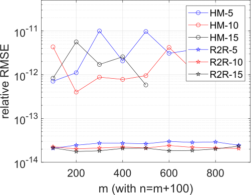
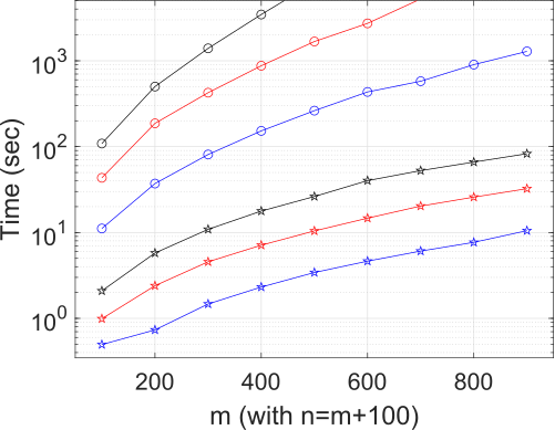
As noted by (Tanner and Wei, 2013), the nuclear norm penalty fails to recover low rank matrices at low oversampling ratios. Recovery in such data-poor settings is possible using non-convex matrix penalties such as the Schatten p𝑝p-norm with p<1𝑝1p<1 (Marjanovic and Solo, 2012; Kümmerle and Sigl, 2018). However, optimizing such norms may be computationally demanding. Figure 1 compares the runtime and recovery error of HM-IRLS optimizing the Schatten p𝑝p-norm with p=1/2𝑝12p=1/2 (Kümmerle and Sigl, 2018) and of our proposed method R2RILS, as a function of matrix size m𝑚m with n=m+100𝑛𝑚100n=m+100. For example, for a rank-10 matrix of size 700×800700800700\times 800, HM-IRLS required over 5000 seconds, whereas R2RILS took about 20 seconds.

The second class consists of iterative methods that strictly enforce the rank r𝑟r constraint of Eq. (1). This includes hard thresholding methods that keep at each iteration only the top r𝑟r singular values and vectors (Tanner and Wei, 2013; Blanchard et al., 2015; Kyrillidis and Cevher, 2014). More related to our work are methods based on a rank r𝑟r factorization Z=UV𝑍𝑈superscript𝑉topZ=UV^{\top} where Um×r𝑈superscript𝑚𝑟U\in\mathbb{R}^{m\times r} and Vn×r𝑉superscript𝑛𝑟V\in\mathbb{R}^{n\times r}. Problem (1) now reads

minU,VUVXF(Ω).subscript𝑈𝑉subscriptnorm𝑈superscript𝑉top𝑋𝐹Ω\min_{U,V}\|UV^{\top}-X\|_{F(\Omega)}. (4)

Whereas Eq. (3) involves mn𝑚𝑛mn optimization variables, problem (4) involves only r(m+n)𝑟𝑚𝑛r(m+n) variables, making it scalable to large matrices.

One approach to optimize Eq. (4) is by alternating minimization (Haldar and Hernando, 2009; Keshavan et al., 2010; Tanner and Wei, 2016; Wen et al., 2012). Each iteration first solves a least squares problem for V𝑉V, keeping the column space estimate U𝑈U fixed. Next, keeping the new V𝑉V fixed, it optimizes over U𝑈U. Under suitable conditions, alternating minimization provably recover the low rank matrix, with high probability (Hardt, 2014; Jain and Netrapalli, 2015; Jain et al., 2013; Keshavan et al., 2010; Sun and Luo, 2016).
Refer to caption
(a) Execution time
Refer to caption
(b) Recovery RMSE
Figure 1: Comparison of HM-IRLS (Kümmerle and Sigl, 2018) and R2RILS for completion of rank r𝑟r matrices of size m×(m+100)𝑚𝑚100m\times(m+100) as a function of m𝑚m, at an oversampling ratio of ρ=2.5𝜌2.5\rho=2.5. For each r{5,10,15}𝑟51015r\in\{5,10,15\}, all non-zero singular values were one. (a) runtime; (b) Relative RMSE on the unobserved entries, Eq. (8). Note that the y𝑦y-axis in both graphs is logarithmic. Results of HM-IRLS at large values of m𝑚m are not shown, as we capped individual runs to 3 hours.

Another iterative approach to optimize (4) was proposed in the 1970’s by Wiberg (Wiberg, 1976), and later became popular in the computer vision community. Given a guess Vtsuperscript𝑉𝑡V^{t}, let U(Vt)𝑈superscript𝑉𝑡U(V^{t}) be the closed form solution to the alternating step of minimizing (4) with respect to U𝑈U. Wiberg’s method writes the new V𝑉V as V=Vt+ΔV𝑉superscript𝑉𝑡Δ𝑉V=V^{t}+\Delta V, and performs a Newton approximation to the functional U(V)VXF(Ω)subscriptnorm𝑈𝑉superscript𝑉top𝑋𝐹Ω\|U(V)V^{\top}-X\|_{F(\Omega)}. This yields a degenerate least squares problem for ΔVΔ𝑉\Delta V. In (Okatani et al., 2011), a damped Wiberg method was proposed with improved convergence and speed.

Yet a different approach to minimize Eq. (4) is via gradient-based Riemannian manifold optimization (Vandereycken, 2013; Boumal and Absil, 2015; Mishra and Sepulchre, 2014; Mishra et al., 2014; Ngo and Saad, 2012). For recovery guarantees of such methods, see (Wei et al., 2016). For scalability to large matrices, (Balzano et al., 2010) devised a stochastic gradient descent approach, called GROUSE, whereas (Recht and Ré, 2013) devised a parallel scheme called JELLYFISH. Finally, uncertainty quantification in noisy matrix completion was recently addressed in (Chen et al., 2019).

While factorization-based methods are fast and scalable, they have two limitations: (i) several of them fail to recover even mildly ill-conditioned low rank matrices and (ii) they require relatively large oversampling ratios to succeed. In applications, the underlying matrices may have a significant spread in their singular values, and clearly the ability to recover a low rank matrix from even a factor of two fewer observations may be of great importance.

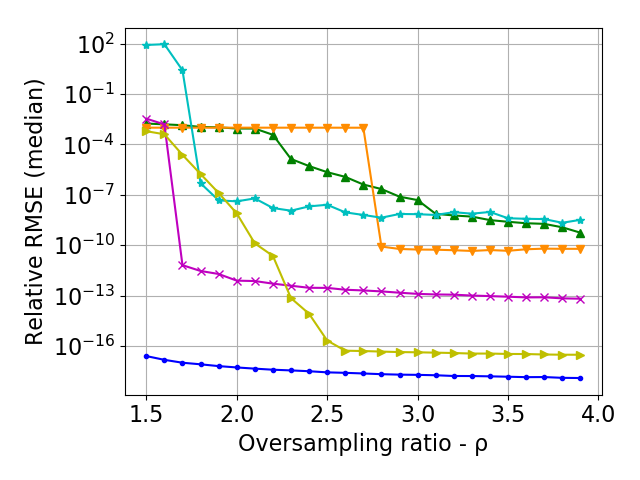
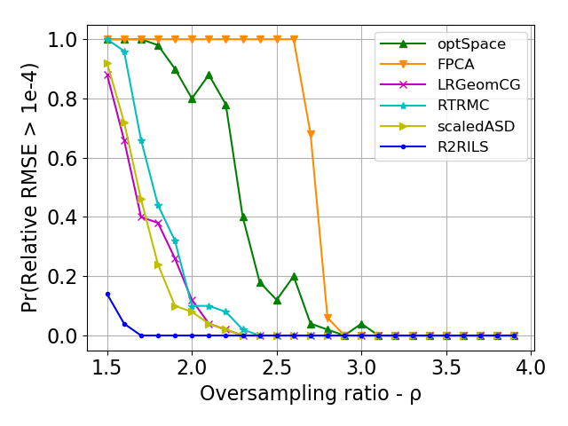
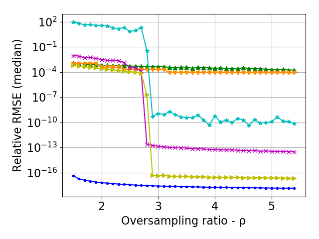
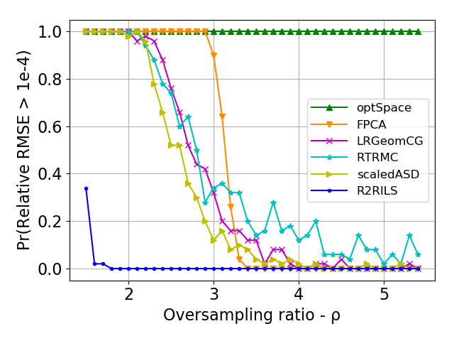
Let us illustrate these two issues. With a full description in Section 3, Figure 2 shows that with a condition number of 1, several popular algorithms recover the low rank matrix. However, as shown in Figure 3, once the condition number is 10, many algorithms either require a high oversampling ratio, or fail to recover the matrix to high accuracy. In contrast, R2RILS recovers the low rank matrices from fewer entries and is less sensitive to the ill conditioning.
Refer to caption
(a) Median of Normalized RMSE
Refer to caption
(b) Failure probability
Figure 2: Comparison of several matrix completion algorithms with well-conditioned matrices of size 1000×1000100010001000\times 1000 and rank r=5𝑟5r=5 as a function of the oversampling ratio ρ𝜌\rho. (a) median of rel-RMSE, Eq. (8); (b) failure probability, defined as rel-RMSE >104absentsuperscript104>10^{-4}. Each point on the two graphs corresponds to 50 independent realizations.

Our Contributions

In this paper, we present R2RILS, a novel iterative method for matrix completion that is simple to implement, computationally efficient, scalable and performs well both with few observations, ill conditioned matrices and noise. Described in Section 2, R2RILS is inspired by factorization algorithms. However, it substantially differs from them, since given a target rank r𝑟r, it does not directly optimize Eq. (4). Instead, we allow our interim matrix to have a specific over-parametrized rank 2r2𝑟2r structure. Optimizing over this rank 2r2𝑟2r matrix yields a least squares problem. At each iteration, R2RILS thus simultaneously optimizes the column and row subspaces. A key step is then an averaging of these new and current estimates.

Section 3 presents an empirical evaluation of R2RILS. First, we consider rank r𝑟r incoherent matrices, with entries observed uniformly at random. We show that in noise-free settings, R2RILS exactly completes matrices from fewer entries than several other low rank completion methods. We further show that R2RILS is robust to ill-conditioning of the underlying matrix and to additive noise. Next, we consider a different type of ill-conditioning, namely power-law matrices which are much less incoherent. Finally, we compare R2RILS to the damped Wiberg’s algorithm on two datasets from computer vision, where the later method was shown to obtain state-of-the-art results. This comparison also highlights some limitations of our method.

To provide insight and motivation for our approach, in Section 4 we study some of its theoretical properties, under the simplified setting of a rank-1 matrix, both with noise free observations as well as with observations corrupted by additive Gaussian noise. While beyond the scope of the current manuscript, we remark that the approach we present in this work can be extended to several other problems, including Poisson low rank matrix completion, one bit matrix completion, and low rank tensor completion. These will be described in future works.
Refer to caption
(a) Median of Normalized RMSE
Refer to caption
(b) Failure probability
Figure 3: Similar comparison as in Fig. 2, but now the rank 555 matrices have singular values 10,8,4,2,110842110,8,4,2,1, resulting in a condition number of 101010.

2 The R2RILS Algorithm

While motivated by factorization methods, a key difference of R2RILS is that it does not directly optimize the objective of Eq. (4). Instead, R2RILS utilizes a specific lifting to the space of rank 2r2𝑟2r matrices. Let (Ut,Vt)subscript𝑈𝑡subscript𝑉𝑡(U_{t},V_{t}) be the estimates of the column and row spaces of the rank r𝑟r matrix X0subscript𝑋0X_{0}, at the start of iteration t𝑡t. Consider the subspace of rank 2r2𝑟2r matrices of the following specific form, with Am×r,Bn×rformulae-sequence𝐴superscript𝑚𝑟𝐵superscript𝑛𝑟A\in\mathbb{R}^{m\times r},B\in\mathbb{R}^{n\times r}.

UtB+AVt,subscript𝑈𝑡superscript𝐵top𝐴superscriptsubscript𝑉𝑡topU_{t}B^{\top}+AV_{t}^{\top},

Starting from an initial guess (U1,V1)subscript𝑈1subscript𝑉1(U_{1},V_{1}) at t=1𝑡1t=1, R2RILS iterates the following two steps:

Step I. Compute the minimal 2subscript2\ell_{2}-norm solution (U~t,V~t)subscript~𝑈𝑡subscript~𝑉𝑡\left(\tilde{U}_{t},\tilde{V}_{t}\right) of the following least squares problem

argminAm×r,Bn×rUtB+AVtXF(Ω).subscriptargminformulae-sequence𝐴superscript𝑚𝑟𝐵superscript𝑛𝑟subscriptnormsubscript𝑈𝑡superscript𝐵top𝐴superscriptsubscript𝑉𝑡top𝑋𝐹Ω\operatorname*{argmin}_{A\in\mathbb{R}^{m\times r},B\in\mathbb{R}^{n\times r}}\|U_{t}B^{\top}+AV_{t}^{\top}-X\|_{F(\Omega)}. (5)

Step II. Update the row and column subspace estimates,

Ut+1=ColNorm(Ut+ColNorm(U~t)),Vt+1=ColNorm(Vt+ColNorm(V~t)),formulae-sequencesubscript𝑈𝑡1ColNormsubscript𝑈𝑡ColNormsubscript~𝑈𝑡subscript𝑉𝑡1ColNormsubscript𝑉𝑡ColNormsubscript~𝑉𝑡\begin{split}U_{t+1}&=\operatorname{ColNorm}\left(U_{t}+\operatorname{ColNorm}\left(\tilde{U}_{t}\right)\right),\\ V_{t+1}&=\operatorname{ColNorm}\left(V_{t}+\operatorname{ColNorm}\left(\tilde{V}_{t}\right)\right),\end{split} (6)

where ColNorm(A)ColNorm𝐴\operatorname{ColNorm}(A) normalizes all r𝑟r columns of the matrix A𝐴A to have unit norm.

1
Input :  ΩΩ\Omega - the set of observed entries.
X𝑋X - an m×n𝑚𝑛m\times n matrix with the observed values in ΩΩ\Omega and zeros in ΩcsuperscriptΩ𝑐\Omega^{c},
r𝑟r - the target rank
U1subscript𝑈1U_{1}, V1subscript𝑉1V_{1} - initial guess for the column and row rank-r subspaces
tmaxsubscript𝑡t_{\max} - maximal number of iterations
Output : X^^𝑋\hat{X} - rank r𝑟r approximation of X𝑋X
2 for  t=1,,tmax𝑡1subscript𝑡t=1,\ldots,t_{\max} do
3       Compute (U~t,V~t)subscript~𝑈𝑡subscript~𝑉𝑡(\tilde{U}_{t},\tilde{V}_{t}), the minimal norm solution of argminAm×r,Bn×rUtB+AVtXF(Ω)subscriptargminformulae-sequence𝐴superscript𝑚𝑟𝐵superscript𝑛𝑟subscriptnormsubscript𝑈𝑡superscript𝐵top𝐴superscriptsubscript𝑉𝑡top𝑋𝐹Ω\operatorname*{argmin}\limits_{A\in\mathbb{R}^{m\times r},B\in\mathbb{R}^{n\times r}}\left\|U_{t}B^{\top}+AV_{t}^{\top}-X\right\|_{F(\Omega)}
4      
5      Ut+1=ColNorm(Ut+ColNorm(U~t))subscript𝑈𝑡1ColNormsubscript𝑈𝑡ColNormsubscript~𝑈𝑡U_{t+1}=\operatorname{ColNorm}\left(U_{t}+\operatorname{ColNorm}\left(\tilde{U}_{t}\right)\right)
6      
7      Vt+1=ColNorm(Vt+ColNorm(V~t))subscript𝑉𝑡1ColNormsubscript𝑉𝑡ColNormsubscript~𝑉𝑡V_{t+1}=\operatorname{ColNorm}\left(V_{t}+\operatorname{ColNorm}\left(\tilde{V}_{t}\right)\right)
8 end for
return X^=^𝑋absent\hat{X}= rank r𝑟r approximation of (UtV~t+U~tVt)subscript𝑈𝑡superscriptsubscript~𝑉𝑡topsubscript~𝑈𝑡superscriptsubscript𝑉𝑡top(U_{t}\tilde{V}_{t}^{\top}+\tilde{U}_{t}V_{t}^{\top}) at the iteration t which achieved the smallest squared error on the observed entries
Algorithm 1 R2RILS

At each iteration we compute the rank r𝑟r projection of the rank-2r2𝑟2r matrix UtV~t+U~tVtsubscript𝑈𝑡superscriptsubscript~𝑉𝑡topsubscript~𝑈𝑡superscriptsubscript𝑉𝑡topU_{t}\tilde{V}_{t}^{\top}+\tilde{U}_{t}V_{t}^{\top} and its squared error on the observed entries. The output of R2RILS is the rank r𝑟r approximation of (UtV~t+U~tVt)subscript𝑈𝑡superscriptsubscript~𝑉𝑡topsubscript~𝑈𝑡superscriptsubscript𝑉𝑡top(U_{t}\tilde{V}_{t}^{\top}+\tilde{U}_{t}V_{t}^{\top}) which minimizes the squared error on the observed entries. A pseudo-code of R2RILS appears in Algorithm 1. As we prove in Lemma 2, if R2RILS converges, then its limiting solution is rank r𝑟r. Next, we provide intuition for R2RILS and discuss some of its differences from other factorization-based methods.

Rank Deficiency. As discussed in Lemma 1 below, Eq. (5) is a rank deficient least squares problem and therefore does not have a unique solution. R2RILS takes the solution with smallest Euclidean norm, which is unique. We remark that the least squares linear system in Wiberg’s method, although different, has a similar rank deficiency, see (Okatani and Deguchi, 2007, Proposition 1).

Simultaneous Row and Column Optimization. In Eq. (5) of Step I, R2RILS finds the best approximation of X𝑋X by a linear combination of the current row and column subspace estimates (Ut,Vt)subscript𝑈𝑡subscript𝑉𝑡(U_{t},V_{t}), using weight matrices (A,B)𝐴𝐵(A,B). Thus, Eq. (5) simultaneously optimizes both the column and row subpaces, generating new estimates for them (U~t,V~t)subscript~𝑈𝑡subscript~𝑉𝑡(\tilde{U}_{t},\tilde{V}_{t}). This scheme is significantly different from alternating minimization methods, which at each step optimize only one of the row or column subspaces, keeping the other fixed. In contrast, R2RILS decouples the estimates, at the expense of lifting to a rank 2r2𝑟2r intermediate solution,

X^t=UtV~t+U~tVt.subscript^𝑋𝑡subscript𝑈𝑡superscriptsubscript~𝑉𝑡topsubscript~𝑈𝑡superscriptsubscript𝑉𝑡top\hat{X}_{t}=U_{t}\tilde{V}_{t}^{\top}+\tilde{U}_{t}V_{t}^{\top}. (7)

Tangent Space. Another prism to look at Eq. (5) is through its connection to the tangent space of the manifold of rank r𝑟r matrices. Consider a rank r𝑟r matrix with column and row subspaces spanned by Utsubscript𝑈𝑡U_{t}, Vtsubscript𝑉𝑡V_{t}, i.e. Z=UtMVt𝑍subscript𝑈𝑡𝑀superscriptsubscript𝑉𝑡topZ=U_{t}MV_{t}^{\top} where Mr×r𝑀superscript𝑟𝑟M\in\mathbb{R}^{r\times r} is invertible. Then the rank 2r2𝑟2r matrix of Eq. (7) is the best approximation of X𝑋X in the tangent space of Z𝑍Z, in least squares sense.

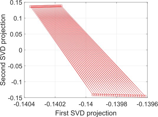
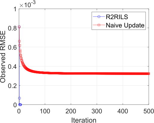
Averaging Current and New Estimates. Since (Ut~,Vt~)~subscript𝑈𝑡~subscript𝑉𝑡(\tilde{U_{t}},\tilde{V_{t}}) can be thought of as new estimates for the column and row spaces, it is tempting to consider the update Ut+1=U~t,Vt+1=V~tformulae-sequencesubscript𝑈𝑡1subscript~𝑈𝑡subscript𝑉𝑡1subscript~𝑉𝑡U_{t+1}=\tilde{U}_{t},V_{t+1}=\tilde{V}_{t}, followed by column normalization. While this update may seem attractive, leading to a non increasing sequence of losses for the objective in Eq. (5), it performs very poorly. Empirically, this update decreases the objective in Eq. (5) extremely slowly, taking thousands of iterations to converge. Moreover, as illustrated in Figure 4, the resulting sequence {(Ut,Vt)}tsubscriptsubscript𝑈𝑡subscript𝑉𝑡𝑡\{(U_{t},V_{t})\}_{t} alternates between two sets of poor estimates. The left panel shows the RMSE on the observed entries versus iteration number for R2RILS, and for a variant whose update is Ut+1=U~t,Vt+1=V~tformulae-sequencesubscript𝑈𝑡1subscript~𝑈𝑡subscript𝑉𝑡1subscript~𝑉𝑡U_{t+1}=\tilde{U}_{t},V_{t+1}=\tilde{V}_{t}, followed by column normalization. Both methods were initialized by the SVD of X𝑋X. While R2RILS converged in 6 iterations, the naive method failed to converge even after 500 iterations. The right panel presents a 2-d visualization of the last 50 vectors Ut,1subscript𝑈𝑡1U_{t,1} under the naive update, as projected into the first and second SVD components of the matrix containing the last 50 values of Utsubscript𝑈𝑡U_{t} for t=451:500:𝑡451500t=451:500. This graph shows an oscillating behavior between two poor vectors. Remark 2 explains this behavior, in the rank-one case.
Refer to caption
Refer to caption
Figure 4: Comparison of R2RILS versus a variant with a naive update. The input is a 400×500400500400\times 500 matrix of rank r=3𝑟3r=3, with observed entries uniformly at random at an oversampling ratio ρ=5𝜌5\rho=5. (a) Observed RMSE as a function of iteration counter. (b) Two dimensional visualization of the oscillating dynamics of Utsubscript𝑈𝑡U_{t} under the naive update rule.

Nonetheless, thinking of (U~t,V~t)subscript~𝑈𝑡subscript~𝑉𝑡(\tilde{U}_{t},\tilde{V}_{t}) as new estimates provides a useful perspective. In particular, if the error in (U~t,V~t)subscript~𝑈𝑡subscript~𝑉𝑡(\tilde{U}_{t},\tilde{V}_{t}) is in a different direction than the error in the initial estimate (Ut,Vt)subscript𝑈𝑡subscript𝑉𝑡(U_{t},V_{t}) or better yet, is approximately in the opposite direction, then the sensible operation to perform is to average these two estimates. This is indeed what R2RILS does in its second step. In Section 4 we show that in the rank-111 case, when the entire matrix is observed, the errors in (U~t,V~t)subscript~𝑈𝑡subscript~𝑉𝑡(\tilde{U}_{t},\tilde{V}_{t}) are indeed approximately in the opposite direction. Furthermore, we show that when the previous estimates are already close to the ground truth, the equal weighting of previous and current estimates is asymptotically optimal. Specifically, this averaging cancels the leading order terms of the errors, and leads to quadratic convergence.

Non-Local Updates. Several Riemannian optimization methods, such as LRGeomCG (Vandereycken, 2013) and RTRMC (Boumal and Absil, 2015), perform local optimization on the manifold of rank r𝑟r matrices, based on the gradient at the current solution. Our update rule is significantly different from these methods, since in Step I, we find the global minimizer of Eq. (5) in a specific rank 2r2𝑟2r subspace. Given the averaging operation in the second step of R2RILS, its next estimate (Ut+1,Vt+1)subscript𝑈𝑡1subscript𝑉𝑡1(U_{t+1},V_{t+1}) may be far from the current one (Ut,Vt)subscript𝑈𝑡subscript𝑉𝑡(U_{t},V_{t}), in particular in the first few iterations.

Invariant Alternatives. An intriguing property of R2RILS is that its next estimate depends explicitly on the specific columns of (Ut,Vt)subscript𝑈𝑡subscript𝑉𝑡(U_{t},V_{t}), and not only on the subspace they span. That is, R2RILS is not invariant to the representation of the current subspace, and does not treat (Ut,Vt)subscript𝑈𝑡subscript𝑉𝑡(U_{t},V_{t}) as elements on the Grassmannian. It is possible to devise variants of R2RILS that are invariant to the subspace representation. One way to do so is to update (Ut+1,Vt+1)subscript𝑈𝑡1subscript𝑉𝑡1(U_{t+1},V_{t+1}) as the average subspace between (Ut,Vt)subscript𝑈𝑡subscript𝑉𝑡(U_{t},V_{t}) and (U~t,V~t)subscript~𝑈𝑡subscript~𝑉𝑡(\tilde{U}_{t},\tilde{V}_{t}), with respect to say the standard Stiefel geometry. Another invariant alternative is to take the best rank r𝑟r approximation of X^tsubscript^𝑋𝑡\hat{X}_{t} from (7) as the next estimate. While these variants work well at high oversampling ratios, the simple column averaging Eq. (6) outperforms them at low oversampling ratios. A theoretical understanding of this behavior is an interesting topic for future research.

Initialization. Similar to other iterative algorithms, R2RILS requires an initial guess U1,V1subscript𝑈1subscript𝑉1U_{1},V_{1}. When the observed entries are distributed uniformly at random, a common choice is to initialize U1,V1subscript𝑈1subscript𝑉1U_{1},V_{1} by the top r𝑟r left and right singular vectors of X𝑋X. As described in (Keshavan et al., 2010), for a trimmed variant of X𝑋X, these quantities are an accurate estimate of the left and right subspaces. In contrast, when the distribution of the observed entries is far from uniform, the rank-r𝑟r SVD of X𝑋X may be a poor initialization, and in various applications, one starts from a random guess, see (Okatani et al., 2011). Empirically, R2RILS performs well also from a random initialization, say with i.i.d. N(0,I)𝑁0𝐼N(0,I) Gaussian vectors, though it may require more iterations to converge. This suggests that the sequence (Ut,Vt)subscript𝑈𝑡subscript𝑉𝑡(U_{t},V_{t}) computed by R2RILS is not attracted to poor local minima. This finding is in accordance with (Ge et al., 2016), that rigorously proved lack of poor local minima for the matrix completion problem under suitable assumptions.

Early Stopping. In the pseudo-code of Algorithm 1, the number of iterations is fixed at tmaxsubscript𝑡t_{\max}. In most of our simulations, we set tmax=300subscript𝑡300t_{\max}=300, though in practice, the algorithm often converged in much fewer iterations. In our code we implemented several early stopping criteria. Let X^rt=SVDr(UtV~+U~Vt)subscriptsuperscript^𝑋𝑡𝑟subscriptSVD𝑟subscript𝑈𝑡superscript~𝑉top~𝑈superscriptsubscript𝑉𝑡top\hat{X}^{t}_{r}=\mbox{SVD}_{r}(U_{t}\tilde{V}^{\top}+\tilde{U}V_{t}^{\top}) denote the rank-r𝑟r approximation of X^tsubscript^𝑋𝑡\hat{X}_{t} from Eq. (7), and let RMSEobst=X^rtXF(Ω)/|Ω|superscriptsubscriptRMSEobs𝑡subscriptnormsubscriptsuperscript^𝑋𝑡𝑟𝑋𝐹ΩΩ\mbox{RMSE}_{\text{obs}}^{t}=\|\hat{X}^{t}_{r}-X\|_{F(\Omega)}/\sqrt{|\Omega|} be the corresponding root mean squared error on the observed entries. Then the first criterion, relevant only to the noise-free case, is

Stop ifRMSEobstϵ,Stop ifsuperscriptsubscriptRMSEobs𝑡italic-ϵ\mbox{Stop if}\qquad\mbox{RMSE}_{\text{obs}}^{t}\leq\epsilon,

taking for instance ϵ1015italic-ϵsuperscript1015\epsilon\leq 10^{-15}. A second stopping criterion, valid also in the noisy case, is

Stop ifX^tX^t1Fmnϵ.Stop ifsubscriptnormsubscript^𝑋𝑡subscript^𝑋𝑡1𝐹𝑚𝑛italic-ϵ\mbox{Stop if}\qquad\frac{\|\hat{X}_{t}-\hat{X}_{t-1}\|_{F}}{\sqrt{mn}}\leq\epsilon.

Finally, a third stopping criterion, useful in particular with real data, is to set δ1much-less-than𝛿1\delta\ll 1 and

Stop if|RMSEobstRMSEobst1|δRMSEobstStop ifsuperscriptsubscriptRMSE𝑜𝑏𝑠𝑡superscriptsubscriptRMSE𝑜𝑏𝑠𝑡1𝛿superscriptsubscriptRMSE𝑜𝑏𝑠𝑡\mbox{Stop if}\qquad|\mbox{RMSE}_{obs}^{t}-\mbox{RMSE}_{obs}^{t-1}|\leq\delta\cdot\mbox{RMSE}_{obs}^{t}

Computational complexity. Our Matlab and Python implementations of R2RILS, available at the author’s website111www.wisdom.weizmann.ac.il/similar-to\simnadler/Projects/R2RILS/, use standard linear algebra packages. Specifically, the minimal norm solution of Eq. (5) is calculated by the LSQR iterative algorithm (Paige and Saunders, 1982). The cost per iteration of LSQR is discussed in (Paige and Saunders, 1982, Section 7.7). In our case, it is dominated by the computation of UtB+AVtsubscript𝑈𝑡superscript𝐵top𝐴superscriptsubscript𝑉𝑡topU_{t}B^{\top}+AV_{t}^{\top} at all entries in ΩΩ\Omega, whose complexity is 𝒪(r|Ω|)𝒪𝑟Ω\mathcal{O}(r|\Omega|). LSQR is mathematically equivalent to conjugate gradient applied to the normal equations. As studied in (Hayami, 2018, Section 4), the residual error after k𝑘k iterations decays like

C(σmaxσminσmax+σmin)k,𝐶superscriptsubscript𝜎subscript𝜎subscript𝜎subscript𝜎𝑘C\left(\frac{\sigma_{\max}-\sigma_{\min}}{\sigma_{\max}+\sigma_{\min}}\right)^{k},

where σmaxsubscript𝜎\sigma_{\max} and σminsubscript𝜎\sigma_{\min} are the largest and smallest non-zero singular values of the rank-deficient matrix of the least squares problem (5). Empirically, at an oversampling ratio ρ=2𝜌2\rho=2 and matrices of size 300×300300300300\times 300, the above quotient is often smaller than 0.90.90.9. Thus, LSQR often requires at most a few hundreds of inner iterations to converge. For larger sized matrices and more challenging instances, more iterations may be needed for a very accurate solution. We capped the maximal number of LSQR iterations at 4000.

Attenuating Non-convergence. On challenging problem instances, where R2RILS fails to find the global minimum solution, empirically the reason is not convergence to a bad local minima. Instead, due to its global updates, (Ut,Vt)subscript𝑈𝑡subscript𝑉𝑡(U_{t},V_{t}) often oscillates in some orbit. To attenuate this behavior, if R2RILS did not coverge within say the first 40 iterations, then once every few iterations we replace the averaging in Eq. (6) with a weighted averaging, which gives more weight to the previous estimate, of the form

Ut+1=ColNorm(βUt+ColNorm(U~t)),subscript𝑈𝑡1ColNorm𝛽subscript𝑈𝑡ColNormsubscript~𝑈𝑡U_{t+1}=\operatorname{ColNorm}\left(\beta U_{t}+\operatorname{ColNorm}\left(\tilde{U}_{t}\right)\right),

and a similar formula for Vt+1subscript𝑉𝑡1V_{t+1}. In our simulations we took β=1+2𝛽12\beta=1+\sqrt{2}. Empirically, this modification increased the cases where R2RILS converged within tmaxsubscript𝑡t_{\max} iterations.

3 Numerical Results

We present simulation results that demonstrate the performance of R2RILS. In the following experiments random matrices were generated according to the uniform model. Specifically, {ui}i=1r,{vi}i=1rsuperscriptsubscriptsubscript𝑢𝑖𝑖1𝑟superscriptsubscriptsubscript𝑣𝑖𝑖1𝑟\{u_{i}\}_{i=1}^{r},\{v_{i}\}_{i=1}^{r} were constructed by drawing r𝑟r vectors uniformly at random from the unit spheres in m,nsuperscript𝑚superscript𝑛\mathbb{R}^{m},\mathbb{R}^{n} respectively and then orthonormalizing them. At every simulation we specify the singular values {σi}i=1rsuperscriptsubscriptsubscript𝜎𝑖𝑖1𝑟\{\sigma_{i}\}_{i=1}^{r} and construct the rank r𝑟r matrix X0subscript𝑋0X_{0} as

X0=i=1rσiuiviT.subscript𝑋0superscriptsubscript𝑖1𝑟subscript𝜎𝑖subscript𝑢𝑖superscriptsubscript𝑣𝑖𝑇X_{0}=\sum_{i=1}^{r}\sigma_{i}u_{i}v_{i}^{T}.

With high probability, the matrix X0subscript𝑋0X_{0} is incoherent (Candès and Recht, 2009). At each oversampling ratio ρ𝜌\rho, we generate a random set ΩΩ\Omega of observed entries by flipping a coin with probability p=ρr(m+nr)(mn)𝑝𝜌𝑟𝑚𝑛𝑟𝑚𝑛p=\rho\cdot\frac{r(m+n-r)}{(m\cdot n)} at each of the mn𝑚𝑛mn matrix entries. The size of ΩΩ\Omega is thus variable and distributed as Binom(mn,p)Binom𝑚𝑛𝑝\mbox{Binom}(m\cdot n,p). As in (Kümmerle and Sigl, 2018), we then verify that each column and row have at least r𝑟r visible entries and repeat this process until this necessary condition for unique recovery is satisfied.

We compare R2RILS with maximal number of iterations tmax=100subscript𝑡100t_{\max}=100 to the following algorithms, using the implementations supplied by the respective authors. As detailed below, for some of them we slightly tuned their parameters to improve their performance.

  • OptSpace (Keshavan et al., 2010): Maximal number of iterations set to 100. Tolerance parameter 1010superscript101010^{-10}.

  • FPCA (Ma et al., 2011): Forced the implementation to use a configuration for ”hard” problem where several parameters are tightened. The two tolerance parameters were set to 1016superscript101610^{-16}.

  • LRGeomCG (Vandereycken, 2013): Executed with its default parameters.

  • RTRMC (Boumal and Absil, 2015): Maximal number of iterations 300, maximal number of inner iterations set to 500. The gradient tolerance was set to 1010superscript101010^{-10}.

  • ScaledASD (Tanner and Wei, 2016): Tolerance parameters 1014superscript101410^{-14} and maximal number of iterations 1000.

  • HM-ILS (Kümmerle and Sigl, 2018): Executed with its default parameters.

We considered two performance measures. The first is the relative RMSE per-entry over the unobserved entries. Given an estimated matrix X^^𝑋\hat{X}, this quantity is defined as

rel-RMSE=mn|Ωc|X^X0F(Ωc)X0F.rel-RMSE𝑚𝑛superscriptΩ𝑐subscriptnorm^𝑋subscript𝑋0𝐹superscriptΩ𝑐subscriptnormsubscript𝑋0𝐹\texttt{rel-RMSE}=\sqrt{\frac{m\cdot n}{|\Omega^{c}|}}\cdot\frac{\|\hat{X}-X_{0}\|_{F(\Omega^{c})}}{\|X_{0}\|_{F}}. (8)

The second measure is the success probability of an algorithm in the ideal setting of noise-free observations. We define success as rel-RMSE<104rel-RMSEsuperscript104\texttt{rel-RMSE}<10^{-4}. This is similar to (Tanner and Wei, 2016), who computed a relative RMSE on all matrix entries, and considered a recovery successful with a slightly looser threshold of 103superscript10310^{-3}. We compare R2RILS to all the above algorithms except for HM-ILS which will be discussed separately. In addition, we also tested the R3MC algorithm (Mishra and Sepulchre, 2014) and the damped Wiberg method of (Okatani et al., 2011). To limit the number of methods shown in the plots of Figs. 2 and 3, the performance of these two methods is not shown in these figures. However, their performance was similar to that of other Riemannian optimization based methods.

Well conditioned setting. In our first experiment, we considered a relatively easy setting with well conditioned matrices of size 1000×1000100010001000\times 1000 and rank r=5𝑟5r=5, whose non zero singular values were all set to 1. Figure 2 shows the reconstruction ability of various algorithms as a function of the oversampling ratio ρ𝜌\rho. In this scenario all algorithms successfully recover the matrix once enough entries are observed. Even in this relatively easy setting, R2RILS shows favorable performance at low oversampling ratios, reaching a relative RMSE around 1014superscript101410^{-14}.

Mild ill-conditioning. Next, we consider a mild ill-conditioning setting, where the rank r=5𝑟5r=5 matrices have a condition number 10, and non-zero singular values 10,8,4,2,110842110,8,4,2,1. As seen in Fig. 3, R2RILS is barely affected by this ill-conditioning and continues to recover the underlying matrix with error 1014superscript101410^{-14} at oversampling ratios larger than 1.51.51.5. In contrast, FPCA, which performs nuclear norm minimization, recovers the matrix at higher oversampling ratios ρ>3.4𝜌3.4\rho>3.4. This is in accordance to similar observations by previous works (Tanner and Wei, 2013; Kümmerle and Sigl, 2018). The other compared algorithms, all of which solve non-convex problems, also require higher oversampling ratios than R2RILS, and even then, occasionally fail to achieve a relative RMSE less than 104superscript10410^{-4}.

Refer to caption
(a) Oversampling 2.5
Refer to caption
(b) Oversampling 3
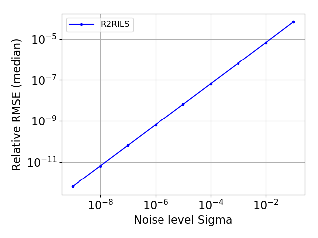
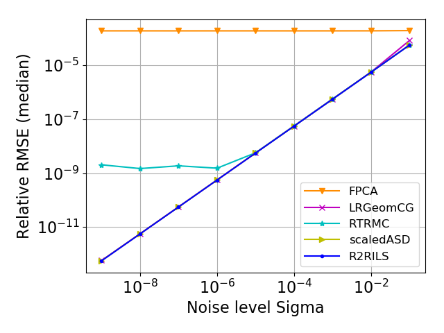
Figure 5: Comparison of several matrix completion algorithms with ill-conditioned matrices and entries corrupted by additive Gaussian noise. Matrices were drawn as in the simulations of Fig. 2. We plot the RMSE per unobserved entry as a function of the standard deviation of the noise. Each point on the graphs corresponds to 50 independent realizations.
Refer to caption
Refer to caption
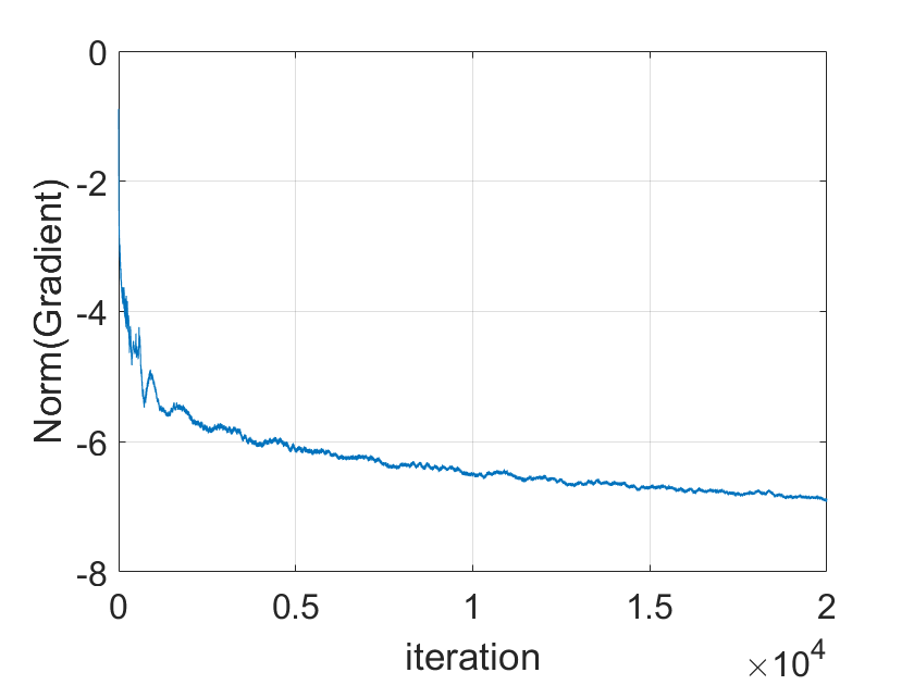
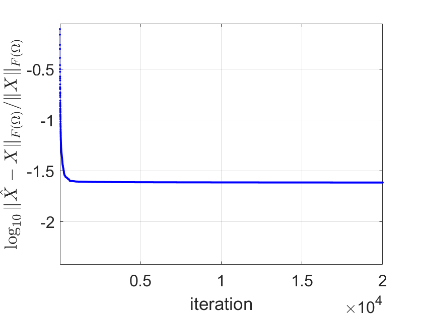
Figure 6: Typical optimization path of LRGeomCG on a 1000×1000100010001000\times 1000 matrix of rank r=5𝑟5r=5, condition number 10, at oversampling ratio ρ=2.2𝜌2.2\rho=2.2. (Left) The norm of the gradient at each iteration on a logarithmic scale. (Right) The normalized error on the observed entries.

Comparison to HM-ILS. The HM-ILS algorithm (Kümmerle and Sigl, 2018) was not included in the above simulations due to its slow runtime. However, from a limited evaluation with smaller sized matrices HM-ILS with Schatten p𝑝p-norm parameter p=1/2𝑝12p=1/2 has excellent performance, comparable to R2RILS, also under ill-conditioning. Figure 1(b) demonstrates that at a low oversampling ratio ρ=2.5𝜌2.5\rho=2.5, both algorithms perfectly reconstruct matrices of various dimensions. Figure 1(a) shows that R2RILS is faster than HM-ILS by orders of magnitude even for modestly sized matrices.

Comparison to Riemannian Manifold Optimization Methods. We considered the optimization path as well as the output of the LRGeomCG algorithm on an instance where it failed to exactly complete the matrix within an increased number of 20000 iterations. Figure 6 shows the norm of the gradient and the normalized error on the observed entries of LRGeomCG versus iteration count. On this instance, the normalized error on the observed entries was 0.0241, whereas on the unobserved entries it was 9.11. It seems that at low oversampling ratios, LRGeomCG converges very slowly to a bad local optimum. Interestingly, starting from this solution of LRGeomCG, R2RILS recovers the low rank matrix within only 20 iterations, with an RMSE of 1013superscript101310^{-13}. We observed the same behavior for 10 different matrices. It thus seems that the lifting to a rank 2r2𝑟2r matrix leads to fewer bad local minima in the optimization landscape. A theoretical study of this issue is an interesting topic for further research.
Refer to caption
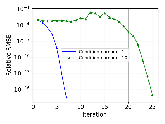
Figure 7: Relative RMSE per observed entry of R2RILS as a function of the iteration number. Each line represents a single execution of R2RILS on a 1000×1000100010001000\times 1000 rank-5 matrix, with oversampling ratio ρ=2.5𝜌2.5\rho=2.5. For the condition-1 matrix all non-zero singular values were set to 1. For the matrix with condition number-10 singular values were set to 10,8,4,2,110842110,8,4,2,1.

Stability to Noise. Figure 5 illustrates the performance of several matrix completion algorithms when i.i.d. zero mean Gaussian noise is added to every observed entry of X0subscript𝑋0X_{0}. As seen in panel 5(a), R2RILS is robust to noise even at low oversampling ratios, with the RMSE linear in the noise level. In Section 4, we prove this result in the case of a fully observed rank-111 matrix. Panel 5(b) shows that most algorithms are also robust to noise, but only at higher oversampling ratios where they start to work in the absence of noise. Algorithms that even without noise failed to recover at an oversampling ratio ρ=3𝜌3\rho=3 are not included in this graph.

Convergence Rate. Figure 7 illustrates the relative RMSE of R2RILS per observed entry, Eq. (8), as a function of the iteration number, on two rank-5 matrices of dimension 1000×1000100010001000\times 1000, oversampling ratio 2.5 and condition numbers 1 and 10. It can be observed that R2RILS’s convergence is very quick once it reaches a small enough error. It is also interesting to note that R2RILS does not monotonically decrease the objective in Eq. (5) at every iteration.

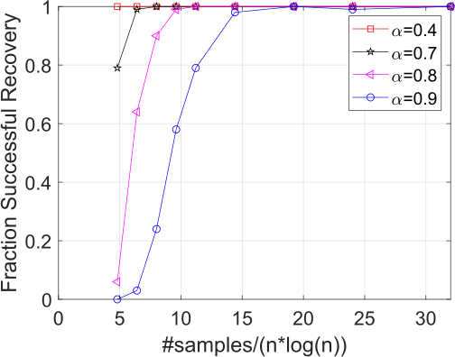
Power-law Matrices. Another form of ill conditioning occurs when the row and/or column subspaces are only weakly incoherent. As in (Chen et al., 2015), we consider power-law matrices of the form X=DUVD𝑋𝐷𝑈superscript𝑉top𝐷X=DUV^{\top}D where the entries of U𝑈U and V𝑉V are i.i.d. 𝒩(0,1)𝒩01\mathcal{N}(0,1) and D=D(α)𝐷𝐷𝛼D=D(\alpha) is a diagonal matrix with power-law decay, Dii=iαsubscript𝐷𝑖𝑖superscript𝑖𝛼D_{ii}=i^{-\alpha}. When α=0𝛼0\alpha=0 the matrix is highly incoherent and relatively easy to recover. When α=1𝛼1\alpha=1 it is highly coherent and more difficult to complete from few entries. Given a budget on the number of observed entries, a 2-step sampling scheme was proposed in (Chen et al., 2015). As shown in (Chen et al., 2015, Fig. 1), 10nlog(n)10𝑛𝑛10n\log(n) adaptively chosen samples were sufficient to recover rank-5 matrices of size 500×500500500500\times 500 by nuclear norm minimization, for values of α0.9𝛼0.9\alpha\leq 0.9. In contrast, with entries observed uniformly at random, nuclear norm minimization required over 300nlog(n)300𝑛𝑛300n\log(n) entries for α0.8𝛼0.8\alpha\geq 0.8. Figure 8 shows the rate of successful recovery (as in (Chen et al., 2015), defined as X^XF/XF0.01subscriptnorm^𝑋𝑋𝐹subscriptnorm𝑋𝐹0.01\|\hat{X}-X\|_{F}/\|X\|_{F}\leq 0.01) by R2RILS as a function of number of entries, chosen uniformly at random while only verifying that each row and column has at least r=5𝑟5r=5 entries. As seen in the figure, R2RILS recovers the underlying matrices with less than 10nlog(n)10𝑛𝑛10n\log(n) entries up to α=0.8𝛼0.8\alpha=0.8, namely without requiring sophisticated adaptive sampling.
Refer to caption
Figure 8: Recovery of power-law matrices by R2RILS.

Datasets from Computer Vision. We conclude the experimental section with results on two benchmark datasets222Datasets available at https://github.com/jhh37/lrmf-datasets/find/master from the computer vision literature (Buchanan and Fitzgibbon, 2005; Hyeong Hong and Fitzgibbon, 2015). We compare R2RILS with the damped Wiberg method333Code downloaded from http://www.vision.is.tohoku.ac.jp/us/download/. The method was run with default parameters as suggested in (Okatani et al., 2011)., which is one of the top performing methods on these benchmarks (Okatani et al., 2011). In these datasets, the goal is to construct a matrix X^^𝑋\hat{X} of given rank r𝑟r, whose RMSE at the observed entries is as small as possible. The observed indices are structured. Hence, the SVD of the observed matrix does not provide an accurate initial guess. Instead, it is common to initialize methods with random U𝑈U and V𝑉V, whose entries are i.i.d. 𝒩(0,1)𝒩01\mathcal{N}(0,1). The quality of an algorithm is assessed by its ability to converge to a solution with low observed RMSE, and by the number of iterations and overall clock time it takes to do so, see (Hyeong Hong and Fitzgibbon, 2015).

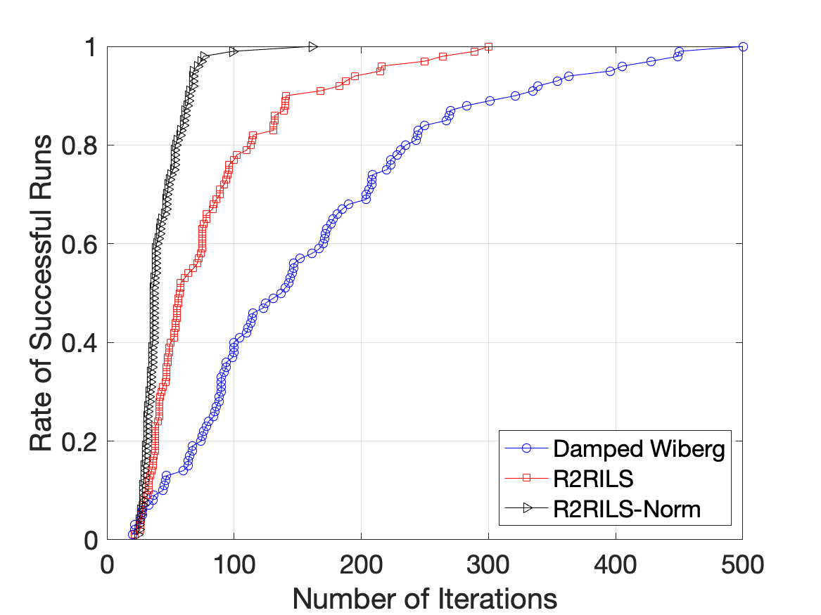
The first dataset is Din (Dino Trimmed in (Hyeong Hong and Fitzgibbon, 2015)), involving the recovery of the rigid turntable motion of a toy dinosaur. The task is to fit a rank r=4𝑟4r=4 matrix of size 72×3197231972\times 319, given 5302 observed entries (23.1%). The best known solution has RMSE 1.084673, and condition number 12.4. Starting from a random guess, R2RILS with maximal number of iterations tmax=300subscript𝑡300t_{\max}=300 achieved this objective in 99/100 runs. The least squares system that R2RILS has to solve is very ill-conditioned for this dataset. We thus also considered a variant, whereby we normalized the columns of the least squares matrix to have unit norm. This variant attained the optimal objective in all 100 runs, and on average converged in fewer number of iterations. Figure 9 (left) shows the cumulative rate of attaining this objective for the three tested algorithms.

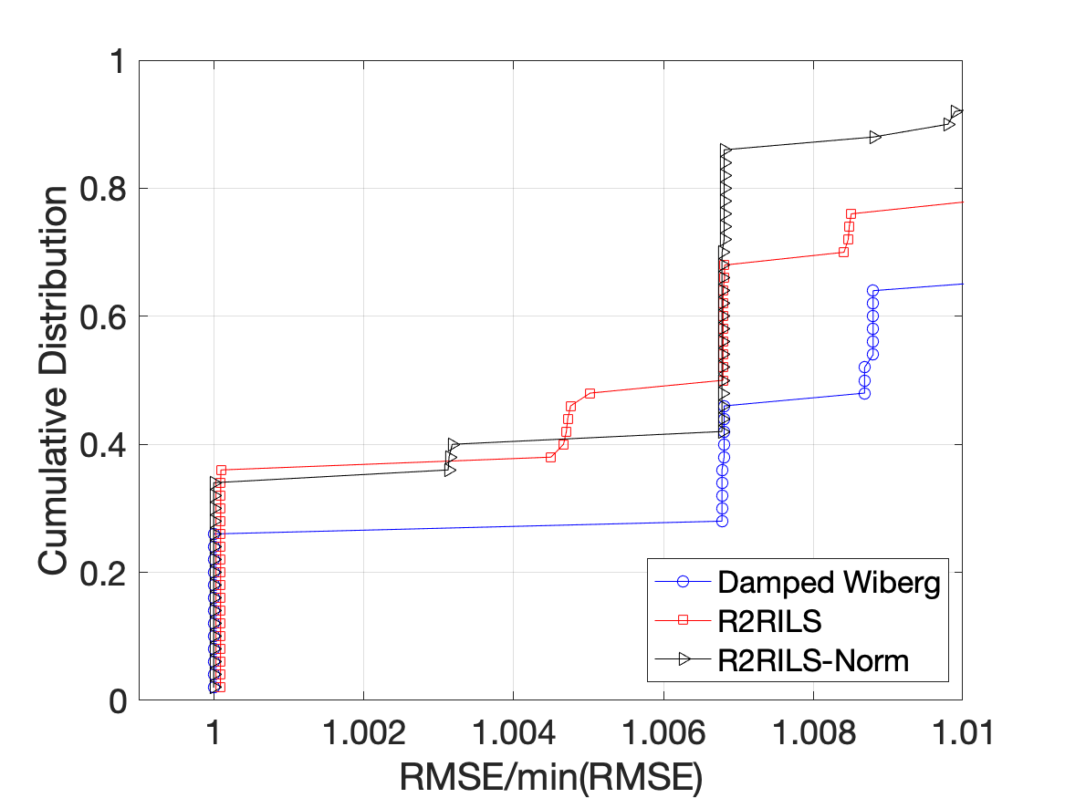
The second dataset is UB4 (Um-boy). Here the task is to fit a rank r=4𝑟4r=4 matrix of size 110×17601101760110\times 1760 given 14.4% of its entries. The best known solution has observed RMSE 1.266484 and condition number 24.5. Out of 50 runs, damped Wiberg attained this RMSE in 13 cases, and the normalized R2RILS variant in 17 runs. The lowest RMSE obtained by R2RILS was slightly higher (1.266597) and this occured in 18 cases. This suggests that R2RILS may be improved by preconditioning the linear system. A practically important remark is that in these datasets, each iteration of damped Wiberg is significantly faster, as it solves a linear system with only rmin(m,n)𝑟𝑚𝑛r\min(m,n) variables, compared to r(m+n)𝑟𝑚𝑛r(m+n) for R2RILS. On the Din dataset, since the ratio n/m4.4𝑛𝑚4.4n/m\approx 4.4, the mean runtime of the normalized variant is only slightly slower than that of damped Wiberg, 17 seconds versus 11 seconds. However, on the UB4 dataset, where n/m=16𝑛𝑚16n/m=16, the clock time of damped Wiberg is significantly faster by a factor of about 60. Developing a variant of R2RILS that solves only for the smaller dimension and would thus be much faster, is an interesting topic for future research.
Refer to caption
Refer to caption
Figure 9: (Left) Cumulative distribution for number of iterations to converge to optimal solution on Din dataset. (Right) Cumulative Distribution of the observed RMSE per entry, divided by the minimal RMSE, on the UB4 dataset, from 50 different random initializations.

4 Theoretical Analysis

We present a preliminary theoretical analysis, which provides both motivation and insight into the two steps of R2RILS. First, Lemma 1 shows that the least squares problem (5) has rank deficiency of dimension at least r2superscript𝑟2r^{2}, similar to Wiberg’s algorithm (Okatani and Deguchi, 2007, Proposition 1). Next, even though R2RILS lifts to rank 2r2𝑟2r matrices, Lemma 2 shows that if it converges, the limiting solution is in fact of rank r𝑟r. Hence, if this solution attains a value of zero for the objective (5), then R2RILS outputs the true underlying matrix X0subscript𝑋0X_{0}. Finally, we study the convergence of R2RILS in the simple rank-1 case. Assuming that the entire matrix is observed, we prove in Theorem 1 that starting from any initial guess weakly correlated to the true singular vectors, R2RILS converges linearly to the underlying matrix. Its proof motivates the averaging step of R2RILS, as it shows that in the rank-1 case, the errors of (U~t,V~t)subscript~𝑈𝑡subscript~𝑉𝑡(\tilde{U}_{t},\tilde{V}_{t}) relative to the true singular vectors are approximately in the opposite direction compared to the errors in (Ut,Vt)subscript𝑈𝑡subscript𝑉𝑡(U_{t},V_{t}). Using this property, we show in Theorem 2 that locally, the convergence of R2RILS is quadratic. Remarks 2 and 3 provide insight and theoretical justification for the equal weighting in the averaging step (6), as well as the choice of the minimal norm solution to the least squares problem (5). Finally, Theorem 3 shows that R2RILS is stable to additive noise, in the fully observed rank-111 case.

Lemma 1.

Suppose that the r𝑟r columns of Utsubscript𝑈𝑡U_{t} and of Vtsubscript𝑉𝑡V_{t} are both linearly independent. Then, the solution space of Eq. (5) has dimension at least r2superscript𝑟2r^{2}. In addition, in the rank-111 case, when Ω=[m]×[n]Ωdelimited-[]𝑚delimited-[]𝑛\Omega=[m]\times[n] the solution space has dimension exactly 111.

Proof.

The solution of (5) is unique up to the kernel of the linear map

(A,B)VecΩ(UtB+AVt)=VecΩ(i=1r(Ut)ibi+ai(Vt)i),maps-to𝐴𝐵subscriptVecΩsubscript𝑈𝑡superscript𝐵top𝐴superscriptsubscript𝑉𝑡topsubscriptVecΩsuperscriptsubscript𝑖1𝑟subscriptsubscript𝑈𝑡𝑖superscriptsubscript𝑏𝑖topsubscript𝑎𝑖superscriptsubscriptsubscript𝑉𝑡𝑖top\displaystyle(A,B)\mapsto\operatorname{Vec}_{\Omega}\left(U_{t}B^{\top}+AV_{t}^{\top}\right)=\operatorname{Vec}_{\Omega}\Big{(}\sum_{i=1}^{r}(U_{t})_{i}b_{i}^{\top}+a_{i}(V_{t})_{i}^{\top}\Big{)}, (9)

where (Ut)isubscriptsubscript𝑈𝑡𝑖(U_{t})_{i} denotes the i𝑖i-th column of U𝑈U and VecΩ(B)|Ω|subscriptVecΩ𝐵superscriptΩ\operatorname{Vec}_{\Omega}(B)\in\mathbb{R}^{|\Omega|} is a vector with entries Bi,jsubscript𝐵𝑖𝑗B_{i,j} for (i,j)Ω𝑖𝑗Ω(i,j)\in\Omega. Choosing ai=j=1rλi,j(Ut)jsubscript𝑎𝑖superscriptsubscript𝑗1𝑟subscript𝜆𝑖𝑗subscriptsubscript𝑈𝑡𝑗a_{i}=\sum_{j=1}^{r}\lambda_{i,j}(U_{t})_{j} and bi=j=1rλj,i(Vt)jsubscript𝑏𝑖superscriptsubscript𝑗1𝑟subscript𝜆𝑗𝑖subscriptsubscript𝑉𝑡𝑗b_{i}=-\sum_{j=1}^{r}\lambda_{j,i}(V_{t})_{j} with r2superscript𝑟2r^{2} free parameters λi,jsubscript𝜆𝑖𝑗\lambda_{i,j} yields an element of the kernel. Hence, the dimension of the kernel is at least r2superscript𝑟2r^{2}.

As for the second part of the lemma, suppose that (a,b)𝑎𝑏(a,b) is a non-trivial solution, such that

utb+avt=0.subscript𝑢𝑡superscript𝑏top𝑎superscriptsubscript𝑣𝑡top0u_{t}b^{\top}+av_{t}^{\top}=0. (10)

Then i𝑖\exists i such that bi0subscript𝑏𝑖0b_{i}\neq 0 and by Eq. (10) biut=(vt)iasubscript𝑏𝑖subscript𝑢𝑡subscriptsubscript𝑣𝑡𝑖𝑎b_{i}u_{t}=-(v_{t})_{i}a, implying that aSpan{ut}𝑎Spansubscript𝑢𝑡a\in\operatorname{Span}\{u_{t}\}. A similar argument shows that bSpan{vt}𝑏Spansubscript𝑣𝑡b\in\operatorname{Span}\{v_{t}\}. Hence the two terms in Eq. (10) take the form utb=λ1utvtsubscript𝑢𝑡superscript𝑏topsubscript𝜆1subscript𝑢𝑡superscriptsubscript𝑣𝑡topu_{t}b^{\top}=\lambda_{1}u_{t}v_{t}^{\top} and avt=λ2utvt𝑎superscriptsubscript𝑣𝑡topsubscript𝜆2subscript𝑢𝑡superscriptsubscript𝑣𝑡topav_{t}^{\top}=\lambda_{2}u_{t}v_{t}^{\top} for some λ1,λ2subscript𝜆1subscript𝜆2\lambda_{1},\lambda_{2}\in\mathbb{R}. For Eq. (10) to hold, λ1=λ2subscript𝜆1subscript𝜆2\lambda_{1}=-\lambda_{2}. Thus, any non trivial solution belongs to the rank-1 subspace λ(ut,vt)𝜆subscript𝑢𝑡subscript𝑣𝑡\lambda(u_{t},-v_{t}). ∎

Lemma 2.

Let rsubscript𝑟\mathcal{M}_{r} be the manifold of m×n𝑚𝑛m\times n rank r𝑟r matrices. Denote by L:r:𝐿subscript𝑟L:\mathcal{M}_{r}\rightarrow\mathbb{R} the squared error loss on the observed entries,

L(Z)=ZXF(Ω)2.𝐿𝑍superscriptsubscriptnorm𝑍𝑋𝐹Ω2L(Z)=\|Z-X\|_{F(\Omega)}^{2}.

Suppose that (Ut,Vt)subscript𝑈𝑡subscript𝑉𝑡(U_{t},V_{t}) is a fixed point of R2RILS, and that the r𝑟r columns of Utsubscript𝑈𝑡U_{t} and of Vtsubscript𝑉𝑡V_{t} are both linearly independent. Then the rank 2r2𝑟2r matrix X^tsubscript^𝑋𝑡\hat{X}_{t} is rank r𝑟r andis a critical point of L𝐿L.

Proof.

Suppose (Ut,Vt)subscript𝑈𝑡subscript𝑉𝑡(U_{t},V_{t}) is a fixed point of R2RILS. Then the solution (U~t,V~t)subscript~𝑈𝑡subscript~𝑉𝑡(\tilde{U}_{t},\tilde{V}_{t}) of Eq. (5) can be written as follows, with diagonal matrices ΣU,ΣVr×rsubscriptΣ𝑈subscriptΣ𝑉superscript𝑟𝑟\Sigma_{U},\Sigma_{V}\in\mathbb{R}^{r\times r},

(U~t,V~t)=(UtΣU,VtΣV)subscript~𝑈𝑡subscript~𝑉𝑡subscript𝑈𝑡subscriptΣ𝑈subscript𝑉𝑡subscriptΣ𝑉(\tilde{U}_{t},\tilde{V}_{t})=(U_{t}\Sigma_{U},V_{t}\Sigma_{V})

This implies that R2RILS’s interim rank 2r2𝑟2r estimate X^tsubscript^𝑋𝑡\hat{X}_{t} of Eq. (7) is in fact of rank r𝑟r, since

X^t=UtΣVVt+UtΣUVt=Ut(ΣU+ΣV)Vt.subscript^𝑋𝑡subscript𝑈𝑡superscriptsubscriptΣ𝑉topsuperscriptsubscript𝑉𝑡topsubscript𝑈𝑡subscriptΣ𝑈superscriptsubscript𝑉𝑡topsubscript𝑈𝑡subscriptΣ𝑈superscriptsubscriptΣ𝑉topsuperscriptsubscript𝑉𝑡top\hat{X}_{t}=U_{t}\Sigma_{V}^{\top}V_{t}^{\top}+U_{t}\Sigma_{U}V_{t}^{\top}=U_{t}(\Sigma_{U}+\Sigma_{V}^{\top})V_{t}^{\top}.

The rank r𝑟r matrix X^tsubscript^𝑋𝑡\hat{X}_{t} is a critical point of the function L𝐿L on the manifold rsubscript𝑟\mathcal{M}_{r} if and only if its gradient L𝐿\nabla L is orthogonal to the tangent space at X^tsubscript^𝑋𝑡\hat{X}_{t}, denoted TX^trsubscript𝑇subscript^𝑋𝑡subscript𝑟T_{\hat{X}_{t}}\mathcal{M}_{r}. Suppose by contradiction that X^tsubscript^𝑋𝑡\hat{X}_{t} is not a critical point of L𝐿L on rsubscript𝑟\mathcal{M}_{r}. Equivalently,

L(X^t)\centernotTX^tr.bottom𝐿subscript^𝑋𝑡\centernotsubscript𝑇subscript^𝑋𝑡subscript𝑟\nabla L(\hat{X}_{t})\centernot{\bot}T_{\hat{X}_{t}}\mathcal{M}_{r}. (11)

The gradient of the loss L𝐿L at a point Z𝑍Z is given by L(Z)=2(PΩ(Z)X)𝐿𝑍2subscript𝑃Ω𝑍𝑋\nabla L(Z)=2\left(P_{\Omega}(Z)-X\right) where PΩsubscript𝑃ΩP_{\Omega} is the projection operator onto the observed entries in the set ΩΩ\Omega,

(PΩ(Z))i,j={Zi,j,if (i,j)Ω,0,otherwise.subscriptsubscript𝑃Ω𝑍𝑖𝑗casessubscript𝑍𝑖𝑗if 𝑖𝑗Ω0otherwise\left(P_{\Omega}(Z)\right)_{i,j}=\begin{cases}Z_{i,j},\quad&\mbox{if }(i,j)\in\Omega,\\ 0,&\mbox{otherwise}.\end{cases}

The tangent space at a point Z=UΣVr𝑍𝑈Σsuperscript𝑉topsubscript𝑟Z=U\Sigma V^{\top}\in\mathcal{M}_{r}, where ΣΣ\Sigma is an invertible r×r𝑟𝑟r\times r matrix, is given by (Vandereycken, 2013, Proposition 2.1)

TZr={UB+AV|Am×r,Bn×r}.subscript𝑇𝑍subscript𝑟conditional-set𝑈superscript𝐵top𝐴superscript𝑉topformulae-sequence𝐴superscript𝑚𝑟𝐵superscript𝑛𝑟\displaystyle T_{Z}\mathcal{M}_{r}=\left\{UB^{\top}+AV^{\top}\;|\;A\in\mathbb{R}^{m\times r},B\in\mathbb{R}^{n\times r}\right\}.

Eq. (11) means that the projection of L(X^t)𝐿subscript^𝑋𝑡\nabla L(\hat{X}_{t}) onto the tangent space TX^tsubscript𝑇subscript^𝑋𝑡T_{\hat{X}_{t}}\mathcal{M} is non trivial. Let UtB+AVtsubscript𝑈𝑡superscript𝐵top𝐴superscriptsubscript𝑉𝑡topU_{t}B^{\top}+AV_{t}^{\top} be this projection. Then

PΩ(X^t)XUtBAVtF<PΩ(X^t)XF.subscriptnormsubscript𝑃Ωsubscript^𝑋𝑡𝑋subscript𝑈𝑡superscript𝐵top𝐴superscriptsubscript𝑉𝑡top𝐹subscriptnormsubscript𝑃Ωsubscript^𝑋𝑡𝑋𝐹\|P_{\Omega}(\hat{X}_{t})-X-U_{t}B^{\top}-AV_{t}^{\top}\|_{F}<\|P_{\Omega}(\hat{X}_{t})-X\|_{F}.

Since PΩ(X^t)subscript𝑃Ωsubscript^𝑋𝑡P_{\Omega}(\hat{X}_{t}) and X𝑋X both vanish on ΩcsuperscriptΩ𝑐\Omega^{c}, the right hand side equals PΩ(X^t)XF(Ω)subscriptnormsubscript𝑃Ωsubscript^𝑋𝑡𝑋𝐹Ω\|P_{\Omega}(\hat{X}_{t})-X\|_{F(\Omega)}. Thus,

PΩ(X^t)XUtBAVtF(Ω)subscriptnormsubscript𝑃Ωsubscript^𝑋𝑡𝑋subscript𝑈𝑡superscript𝐵top𝐴superscriptsubscript𝑉𝑡top𝐹Ω\displaystyle\|P_{\Omega}(\hat{X}_{t})-X-U_{t}B^{\top}-AV_{t}^{\top}\|_{F(\Omega)} PΩ(X^t)XUtBAVtF<PΩ(X^t)XF(Ω).absentsubscriptnormsubscript𝑃Ωsubscript^𝑋𝑡𝑋subscript𝑈𝑡superscript𝐵top𝐴superscriptsubscript𝑉𝑡top𝐹subscriptnormsubscript𝑃Ωsubscript^𝑋𝑡𝑋𝐹Ω\displaystyle\leq\|P_{\Omega}(\hat{X}_{t})-X-U_{t}B^{\top}-AV_{t}^{\top}\|_{F}<\|P_{\Omega}(\hat{X}_{t})-X\|_{F(\Omega)}.

This contradicts the assumption that (U~t,V~t)subscript~𝑈𝑡subscript~𝑉𝑡(\tilde{U}_{t},\tilde{V}_{t}) is a global minimizer of Eq. (5). ∎

Corollary 1.

Consider a noise-free matrix completion problem with an underlying matrix X0subscript𝑋0X_{0} of rank r𝑟r and a set Ω[m]×[n]Ωdelimited-[]𝑚delimited-[]𝑛\Omega\subset[m]\times[n] such that the solution to (1) is unique. If R2RILS converged to a fixed point (Ut,Vt)subscript𝑈𝑡subscript𝑉𝑡(U_{t},V_{t}) with a zero value for the least squares objective (5), UtV~t+U~tVtXF(Ω)=0subscriptnormsubscript𝑈𝑡superscriptsubscript~𝑉𝑡topsubscript~𝑈𝑡superscriptsubscript𝑉𝑡top𝑋𝐹Ω0\left\|U_{t}\tilde{V}_{t}^{\top}+\tilde{U}_{t}V_{t}^{\top}-X\right\|_{F(\Omega)}=0, then its output is the true underlying matrix X0subscript𝑋0X_{0}.

Proof.

By Lemma 2, if R2RILS converged then the intermediate matrix UtV~t+U~tVtsubscript𝑈𝑡superscriptsubscript~𝑉𝑡topsubscript~𝑈𝑡superscriptsubscript𝑉𝑡topU_{t}\tilde{V}_{t}^{\top}+\tilde{U}_{t}V_{t}^{\top} is in fact rank-r𝑟r. As this matrix attains a zero value for the objective (1), it equals X0subscript𝑋0X_{0}. ∎

Next, we study the convergence of R2RILS, in the simple case where X0=σuvsubscript𝑋0𝜎𝑢superscript𝑣topX_{0}=\sigma uv^{\top} is of rank-1, and assume that we have observed all entries of X0subscript𝑋0X_{0}. These two assumptions allow us to find a closed form solution to the least squares problem and are critical for our proof analysis. It may be possible to extend our proof to higher rank settings and to partially observed matrices with a more complicated proof. We leave this for future work.

Let (ut,vt)subscript𝑢𝑡subscript𝑣𝑡(u_{t},v_{t}) be the estimates of R2R2ILS at iteration t𝑡t. In the rank-111 case utsubscript𝑢𝑡u_{t} and vtsubscript𝑣𝑡v_{t} are vectors and we may decompose each of them into two components. The first is their projection on the true (u,v)𝑢𝑣(u,v), and the second is the orthogonal complement which is their error,

ut=αtu+1αt2eu,t,vt=βtv+1βt2ev,t.formulae-sequencesubscript𝑢𝑡subscript𝛼𝑡𝑢1superscriptsubscript𝛼𝑡2subscript𝑒𝑢𝑡subscript𝑣𝑡subscript𝛽𝑡𝑣1superscriptsubscript𝛽𝑡2subscript𝑒𝑣𝑡u_{t}=\alpha_{t}u+\sqrt{1-\alpha_{t}^{2}}e_{u,t}\;,\;v_{t}=\beta_{t}v+\sqrt{1-\beta_{t}^{2}}e_{v,t}. (12)

For future use we define ϵt=1αt2subscriptitalic-ϵ𝑡1superscriptsubscript𝛼𝑡2\epsilon_{t}=\sqrt{1-\alpha_{t}^{2}}, δt=1βt2subscript𝛿𝑡1superscriptsubscript𝛽𝑡2\delta_{t}=\sqrt{1-\beta_{t}^{2}}, and the following two quantities

h(ϵ)=1+2ϵ23ϵ4,r(ϵ)=1+ϵ2+h(ϵ)2(1+3ϵ2+h(ϵ)).formulae-sequenceitalic-ϵ12superscriptitalic-ϵ23superscriptitalic-ϵ4𝑟italic-ϵ1superscriptitalic-ϵ2italic-ϵ213superscriptitalic-ϵ2italic-ϵh(\epsilon)=\sqrt{1+2\epsilon^{2}-3\epsilon^{4}},\quad\quad r(\epsilon)=\frac{1+\epsilon^{2}+h(\epsilon)}{\sqrt{2(1+3\epsilon^{2}+h(\epsilon))}}. (13)

Note that both (u,v)𝑢𝑣(u,v) and hence also (αt,βt)subscript𝛼𝑡subscript𝛽𝑡(\alpha_{t},\beta_{t}) are determined up a joint ±1plus-or-minus1\pm 1 sign. In the following, we will assume that the initial guess satisfies sign(α1)=sign(β1)>0signsubscript𝛼1signsubscript𝛽10\text{sign}(\alpha_{1})=\text{sign}(\beta_{1})>0.

The first theorem below shows that in the fully-observed rank-1 case, from any initial guess weakly correlated to the true singular vectors (α1,β1>0subscript𝛼1subscript𝛽10\alpha_{1},\beta_{1}>0), R2RILS converges linearly to the matrix X0subscript𝑋0X_{0}. The second theorem shows that asymptotically, the convergence is quadratic.

Theorem 1.

Assume that Ω=[m]×[n]Ωdelimited-[]𝑚delimited-[]𝑛\Omega=[m]\times[n], and that the initial guess (u1,v1)subscript𝑢1subscript𝑣1(u_{1},v_{1}) satisfies α1,β1>0subscript𝛼1subscript𝛽10\alpha_{1},\beta_{1}>0. Then the sequence of estimates (ut,vt)subscript𝑢𝑡subscript𝑣𝑡(u_{t},v_{t}) generated by R2RILS converges to (u,v)𝑢𝑣(u,v) linearly with a contraction factor smaller than 1120.541120.54\sqrt{1-\frac{1}{\sqrt{2}}}\approx 0.54. Specifically,

(ut+1vt+1)(uv)=R(ϵt,δt)(utvt)(uv)normmatrixsubscript𝑢𝑡1subscript𝑣𝑡1matrix𝑢𝑣𝑅subscriptitalic-ϵ𝑡subscript𝛿𝑡normmatrixsubscript𝑢𝑡subscript𝑣𝑡matrix𝑢𝑣\displaystyle\left\|\begin{pmatrix}u_{t+1}\\ v_{t+1}\end{pmatrix}-\begin{pmatrix}u\\ v\end{pmatrix}\right\|=R(\epsilon_{t},\delta_{t})\left\|\begin{pmatrix}u_{t}\\ v_{t}\end{pmatrix}-\begin{pmatrix}u\\ v\end{pmatrix}\right\| (14)

where

R(ϵt,δt)=[2r(ϵt)r(δt)21ϵt21δt2]12112max{ϵt,δt},𝑅subscriptitalic-ϵ𝑡subscript𝛿𝑡superscriptdelimited-[]2𝑟subscriptitalic-ϵ𝑡𝑟subscript𝛿𝑡21superscriptsubscriptitalic-ϵ𝑡21superscriptsubscript𝛿𝑡212112subscriptitalic-ϵ𝑡subscript𝛿𝑡R(\epsilon_{t},\delta_{t})=\left[\frac{2-r(\epsilon_{t})-r(\delta_{t})}{2-\sqrt{1-\epsilon_{t}^{2}}-\sqrt{1-\delta_{t}^{2}}}\right]^{\frac{1}{2}}\leq\sqrt{1-\frac{1}{\sqrt{2}}}\max\{\epsilon_{t},\delta_{t}\},

and the function r(ϵ)𝑟italic-ϵr(\epsilon) was defined in Eq. (13) above.

Theorem 2.

As ϵt,δt0subscriptitalic-ϵ𝑡subscript𝛿𝑡0\epsilon_{t},\delta_{t}\to 0, the convergence is quadratic, with an asymptotic contraction factor of ϵt4ϵt2δt2+δt42max{ϵt2,δt2}superscriptsubscriptitalic-ϵ𝑡4superscriptsubscriptitalic-ϵ𝑡2superscriptsubscript𝛿𝑡2superscriptsubscript𝛿𝑡42superscriptsubscriptitalic-ϵ𝑡2superscriptsubscript𝛿𝑡2\sqrt{\epsilon_{t}^{4}-\epsilon_{t}^{2}\delta_{t}^{2}+\delta_{t}^{4}}\leq\sqrt{2}\max\{\epsilon_{t}^{2},\delta_{t}^{2}\}.

Remark 1.

In the fully observed rank-1 case, it follows from the proof of Theorem 1 and can also be observed empirically that if the initial guess (u1,v1)subscript𝑢1subscript𝑣1(u_{1},v_{1}) is misaligned with the singular vectors (u,v)𝑢𝑣(u,v), namely α1β1<0subscript𝛼1subscript𝛽10\alpha_{1}\cdot\beta_{1}<0, then R2RILS fails to converge. However, this has little practical significance, since if only some entries are observed and/or the rank is higher then with enough observed entries, empirically R2RILS converges to the exact low rank matrix.

Next, we present two remarks that theoretically motivate the choice of the minimal norm solution and the averaging step of R2RILS, both in the fully observed rank-111 case.

Remark 2.

Consider a variant of R2RILS, where step II is replaced by

ut+1=ColNorm(ut+wuColNorm(u~t)),vt+1=ColNorm(vt+wvColNorm(v~t)),formulae-sequencesubscript𝑢𝑡1ColNormsubscript𝑢𝑡subscript𝑤𝑢ColNormsubscript~𝑢𝑡subscript𝑣𝑡1ColNormsubscript𝑣𝑡subscript𝑤𝑣ColNormsubscript~𝑣𝑡\displaystyle\begin{aligned} u_{t+1}=\operatorname{ColNorm}\left(u_{t}+w_{u}\cdot\operatorname{ColNorm}\left(\tilde{u}_{t}\right)\right),\,v_{t+1}=\operatorname{ColNorm}\left(v_{t}+w_{v}\cdot\operatorname{ColNorm}\left(\tilde{v}_{t}\right)\right),\end{aligned} (15)

with weights wu,wvsubscript𝑤𝑢subscript𝑤𝑣w_{u},w_{v}\in\mathbb{R} that possibly depend on t𝑡t. In the case Ω=[m]×[n]Ωdelimited-[]𝑚delimited-[]𝑛\Omega=[m]\times[n] and α1,β1>0subscript𝛼1subscript𝛽10\alpha_{1},\beta_{1}>0, it is possible to converge to the exact rank-111 matrix X0subscript𝑋0X_{0} after a single iteration, by setting

wu=(utColNorm(u~t))1,wv=(vtColNorm(v~t))1.formulae-sequencesubscript𝑤𝑢superscriptsuperscriptsubscript𝑢𝑡topColNormsubscript~𝑢𝑡1subscript𝑤𝑣superscriptsuperscriptsubscript𝑣𝑡topColNormsubscript~𝑣𝑡1\displaystyle\begin{aligned} w_{u}=\left(u_{t}^{\top}\operatorname{ColNorm}\left(\tilde{u}_{t}\right)\right)^{-1},\quad w_{v}=\left(v_{t}^{\top}\operatorname{ColNorm}\left(\tilde{v}_{t}\right)\right)^{-1}.\end{aligned} (16)

Note that as ϵt,δt0subscriptitalic-ϵ𝑡subscript𝛿𝑡0\epsilon_{t},\delta_{t}\to 0, namely as the current estimate becomes closer to (u,v)𝑢𝑣(u,v), then the optimal weights satisfy wu,wv1subscript𝑤𝑢subscript𝑤𝑣1w_{u},w_{v}\to 1, resulting in the original R2RILS. In other words, the averaging step of R2RILS is asymptotically optimal in the fully observed rank-1 case.

Remark 3.

Assume Ω=[m]×[n]Ωdelimited-[]𝑚delimited-[]𝑛\Omega=[m]\times[n] and let X=σuv𝑋𝜎𝑢superscript𝑣topX=\sigma uv^{\top}. By the proof of Lemma 2, in this case, the kernel of the linear map (9) is rank one, spanned by (ut,vt)subscript𝑢𝑡subscript𝑣𝑡(u_{t},-v_{t}). Consider a variant where in step I, instead of the minimal norm solution (u~t,v~t)subscript~𝑢𝑡subscript~𝑣𝑡(\tilde{u}_{t},\tilde{v}_{t}), it takes a solution of the form

(u^tv^t)=(u~tv~t)+λt(utvt)matrixsubscript^𝑢𝑡subscript^𝑣𝑡matrixsubscript~𝑢𝑡subscript~𝑣𝑡subscript𝜆𝑡matrixsubscript𝑢𝑡subscript𝑣𝑡\begin{pmatrix}\hat{u}_{t}\\ \hat{v}_{t}\end{pmatrix}=\begin{pmatrix}\tilde{u}_{t}\\ \tilde{v}_{t}\end{pmatrix}+\lambda_{t}\begin{pmatrix}u_{t}\\ -v_{t}\end{pmatrix}

where the scalar λtsubscript𝜆𝑡\lambda_{t} may in general depend on ut,vtsubscript𝑢𝑡subscript𝑣𝑡u_{t},v_{t} and on t𝑡t. Assume that (ut,vt)subscript𝑢𝑡subscript𝑣𝑡(u_{t},v_{t}) are aligned with (u,v)𝑢𝑣(u,v), namely αt,βt>0subscript𝛼𝑡subscript𝛽𝑡0\alpha_{t},\beta_{t}>0. Then, the only choice that leads to quadratic convergence of the column or row space as ϵt0subscriptitalic-ϵ𝑡0\epsilon_{t}\to 0 or δt0subscript𝛿𝑡0\delta_{t}\to 0 is the minimal norm solution, namely λt=0subscript𝜆𝑡0\lambda_{t}=0.

Finally, the following theorem shows that in the presence of additive Gaussian noise, the estimates (ut,vt)subscript𝑢𝑡subscript𝑣𝑡(u_{t},v_{t}) of R2RILS are close to the true vectors (u,v)𝑢𝑣(u,v) up to an error term linear in the noise level. A similar result, with different constants, also holds for sub-Gaussian noise.

Theorem 3.

Let Ω=[m]×[n]Ωdelimited-[]𝑚delimited-[]𝑛\Omega=[m]\times[n], and assume w.l.o.g. that ρmn1𝜌𝑚𝑛1\rho\equiv\sqrt{\frac{m}{n}}\leq 1. Let X=σuv+Z𝑋𝜎𝑢superscript𝑣top𝑍X=\sigma uv^{\top}+Z where σ>0𝜎0\sigma>0, u=v=1norm𝑢norm𝑣1\|u\|=\|v\|=1 and all entries Zi,jsubscript𝑍𝑖𝑗Z_{i,j} are i.i.d. Gaussian with mean 0 and variance η02superscriptsubscript𝜂02\eta_{0}^{2}. Let δ(0,14]𝛿014\delta\in\left(0,\frac{1}{4}\right], and assume the initial guess of R2RILS, (u1,v1)subscript𝑢1subscript𝑣1(u_{1},v_{1}), satisfies α1,β1δsubscript𝛼1subscript𝛽1𝛿\alpha_{1},\beta_{1}\geq\delta. Denote the normalized noise level ηη0n𝜂subscript𝜂0𝑛\eta\equiv\eta_{0}\sqrt{n}, and the constants R1120.54𝑅112similar-to-or-equals0.54R\equiv\sqrt{1-\frac{1}{\sqrt{2}}}\simeq 0.54, C501R𝐶501𝑅C\equiv\frac{50}{1-R}. If

ησ2Cδ,𝜂𝜎2𝐶𝛿\displaystyle\frac{\eta}{\sigma}\leq\frac{\sqrt{2}}{C}\cdot\delta, (17)

then with probability at least 1en21superscript𝑒𝑛21-e^{-\frac{n}{2}}, for all t2𝑡2t\geq 2,

(utvt)(uv)normmatrixsubscript𝑢𝑡subscript𝑣𝑡matrix𝑢𝑣\displaystyle\left\|\begin{pmatrix}u_{t}\\ v_{t}\end{pmatrix}-\begin{pmatrix}u\\ v\end{pmatrix}\right\| 3Rt2+4C(1Rt2)ησ.absent3superscript𝑅𝑡24𝐶1superscript𝑅𝑡2𝜂𝜎\displaystyle\leq\sqrt{3}R^{t-2}+4C\left(1-R^{t-2}\right)\frac{\eta}{\sigma}. (18)

Hence, after log(η/σ)𝜂𝜎\log(\eta/\sigma) iterations, the error is O(η/σ)𝑂𝜂𝜎O(\eta/\sigma).

We first present the proof of Theorem 2 assuming Theorem 1 holds, and then present the proof of the latter. The proof of Theorem 3 appears in Appendix A.

Proof of Theorem 2.

Since h(ϵ)=1+ϵ22ϵ4+2ϵ6+𝒪(ϵ8)italic-ϵ1superscriptitalic-ϵ22superscriptitalic-ϵ42superscriptitalic-ϵ6𝒪superscriptitalic-ϵ8h(\epsilon)=1+\epsilon^{2}-2\epsilon^{4}+2\epsilon^{6}+\mathcal{O}\left(\epsilon^{8}\right), it follows that r(ϵ)=112ϵ6+𝒪(ϵ8)𝑟italic-ϵ112superscriptitalic-ϵ6𝒪superscriptitalic-ϵ8r(\epsilon)=1-\frac{1}{2}\epsilon^{6}+\mathcal{O}\left(\epsilon^{8}\right). Substituting these Taylor expansions into R(ϵt,δt)𝑅subscriptitalic-ϵ𝑡subscript𝛿𝑡R(\epsilon_{t},\delta_{t}) gives

R(ϵt,δt)=[ϵt6+δt6+𝒪(ϵt8)+𝒪(δt8)ϵt2+δt2+𝒪(ϵt4)+𝒪(δt4)]12=ϵt4ϵt2δt2+δt4(1+o(1)).𝑅subscriptitalic-ϵ𝑡subscript𝛿𝑡superscriptdelimited-[]superscriptsubscriptitalic-ϵ𝑡6superscriptsubscript𝛿𝑡6𝒪superscriptsubscriptitalic-ϵ𝑡8𝒪superscriptsubscript𝛿𝑡8superscriptsubscriptitalic-ϵ𝑡2superscriptsubscript𝛿𝑡2𝒪superscriptsubscriptitalic-ϵ𝑡4𝒪superscriptsubscript𝛿𝑡412superscriptsubscriptitalic-ϵ𝑡4superscriptsubscriptitalic-ϵ𝑡2superscriptsubscript𝛿𝑡2superscriptsubscript𝛿𝑡41𝑜1R(\epsilon_{t},\delta_{t})=\left[\frac{\epsilon_{t}^{6}+\delta_{t}^{6}+\mathcal{O}\left(\epsilon_{t}^{8}\right)+\mathcal{O}\left(\delta_{t}^{8}\right)}{\epsilon_{t}^{2}+\delta_{t}^{2}+\mathcal{O}\left(\epsilon_{t}^{4}\right)+\mathcal{O}\left(\delta_{t}^{4}\right)}\right]^{\frac{1}{2}}=\sqrt{\epsilon_{t}^{4}-\epsilon_{t}^{2}\delta_{t}^{2}+\delta_{t}^{4}}\,\cdot(1+o(1)).

To prove Theorem 1, we use the following lemma which provides a closed form expression to the minimal norm solution of Eq. (5), in the rank-1 case where all entries of the matrix have been observed. The proof of this auxiliary lemma appears in Appendix B.

Lemma 3.

Assume that Ω=[m]×[n]Ωdelimited-[]𝑚delimited-[]𝑛\Omega=[m]\times[n]. Given non-zero vectors (ut,vt)m×nsubscript𝑢𝑡subscript𝑣𝑡superscript𝑚superscript𝑛(u_{t},v_{t})\in\mathbb{R}^{m}\times\mathbb{R}^{n} and an observed matrix X𝑋X, the minimal norm solution to the least squares problem (5) is

u~=1vt2(XvtutXvtNtut),v~=1ut2(XututXvtNtvt).formulae-sequence~𝑢1superscriptnormsubscript𝑣𝑡2𝑋subscript𝑣𝑡superscriptsubscript𝑢𝑡top𝑋subscript𝑣𝑡subscript𝑁𝑡subscript𝑢𝑡~𝑣1superscriptnormsubscript𝑢𝑡2superscript𝑋topsubscript𝑢𝑡superscriptsubscript𝑢𝑡top𝑋subscript𝑣𝑡subscript𝑁𝑡subscript𝑣𝑡\displaystyle\tilde{u}=\frac{1}{\|{v}_{t}\|^{2}}\left(X{v}_{t}-\frac{{u}_{t}^{\top}X{v}_{t}}{N_{t}}{u}_{t}\right),\quad\tilde{v}=\frac{1}{\|u_{t}\|^{2}}\left(X^{\top}{u}_{t}-\frac{{u}_{t}^{\top}X{v}_{t}}{N_{t}}{v}_{t}\right). (19)

where Nt=ut2+vt2subscript𝑁𝑡superscriptnormsubscript𝑢𝑡2superscriptnormsubscript𝑣𝑡2N_{t}=\|u_{t}\|^{2}+\|v_{t}\|^{2}. If the matrix X𝑋X is rank-one, X=σuv𝑋𝜎𝑢superscript𝑣topX=\sigma uv^{\top} with σ>0𝜎0\sigma>0, and all vectors are normalized, u=v=ut=vt=1norm𝑢norm𝑣normsubscript𝑢𝑡normsubscript𝑣𝑡1\|u\|=\|v\|=\|u_{t}\|=\|{v}_{t}\|=1, Eq. (19) simplifies to

u~=(u12αtut)βtσ,v~=(v12βtvt)αtσformulae-sequence~𝑢𝑢12subscript𝛼𝑡subscript𝑢𝑡subscript𝛽𝑡𝜎~𝑣𝑣12subscript𝛽𝑡subscript𝑣𝑡subscript𝛼𝑡𝜎\displaystyle\begin{aligned} \tilde{u}=\left(u-\tfrac{1}{2}\alpha_{t}u_{t}\right)\beta_{t}\sigma,\quad\tilde{v}=\left(v-\tfrac{1}{2}\beta_{t}v_{t}\right)\alpha_{t}\sigma\end{aligned} (20)

where αt=uutsubscript𝛼𝑡superscript𝑢topsubscript𝑢𝑡\alpha_{t}={u}^{\top}{u}_{t} and βt=vvtsubscript𝛽𝑡superscript𝑣topsubscript𝑣𝑡\beta_{t}=v^{\top}{v}_{t}.

Proof of Theorem 1.

It follows from Lemma 3, that the result of step I of R2RILS is given by Eq. (20). The normalized result is thus

ColNorm(u~t)=u12αtutα~tsign(βt),ColNorm(v~t)=v12βtvtβ~tsign(αt),formulae-sequenceColNormsubscript~𝑢𝑡𝑢12subscript𝛼𝑡subscript𝑢𝑡subscript~𝛼𝑡signsubscript𝛽𝑡ColNormsubscript~𝑣𝑡𝑣12subscript𝛽𝑡subscript𝑣𝑡subscript~𝛽𝑡signsubscript𝛼𝑡\displaystyle\operatorname{ColNorm}\left(\tilde{u}_{t}\right)=\frac{u-\frac{1}{2}\alpha_{t}u_{t}}{\tilde{\alpha}_{t}}\text{sign}(\beta_{t}),\quad\operatorname{ColNorm}\left(\tilde{v}_{t}\right)=\frac{v-\frac{1}{2}\beta_{t}v_{t}}{\tilde{\beta}_{t}}\text{sign}(\alpha_{t}), (21)

where α~t=13αt24subscript~𝛼𝑡13superscriptsubscript𝛼𝑡24\tilde{\alpha}_{t}=\sqrt{1-\frac{3\alpha_{t}^{2}}{4}} and β~t=13βt24subscript~𝛽𝑡13superscriptsubscript𝛽𝑡24\tilde{\beta}_{t}=\sqrt{1-\frac{3\beta_{t}^{2}}{4}}. Assume for now that αt,βt>0subscript𝛼𝑡subscript𝛽𝑡0\alpha_{t},\beta_{t}>0. Later we will prove that α1,β1>0subscript𝛼1subscript𝛽10\alpha_{1},\beta_{1}>0 indeed implies αt,βt>0subscript𝛼𝑡subscript𝛽𝑡0\alpha_{t},\beta_{t}>0 for all t1𝑡1t\geq 1. Then the next estimate is

ut+1subscript𝑢𝑡1\displaystyle u_{t+1} =ColNorm(ut+ColNorm(u~t))=u+(α~t12αt)ut232αt2+αtα~tabsentColNormsubscript𝑢𝑡ColNormsubscript~𝑢𝑡𝑢subscript~𝛼𝑡12subscript𝛼𝑡subscript𝑢𝑡232superscriptsubscript𝛼𝑡2subscript𝛼𝑡subscript~𝛼𝑡\displaystyle=\operatorname{ColNorm}\left(u_{t}+\operatorname{ColNorm}(\tilde{u}_{t})\right)=\frac{u+(\tilde{\alpha}_{t}-\frac{1}{2}\alpha_{t})u_{t}}{\sqrt{2-\frac{3}{2}\alpha_{t}^{2}+\alpha_{t}\tilde{\alpha}_{t}}}

with a similar expression for vt+1subscript𝑣𝑡1v_{t+1}. Their projections on the true vectors are

αt+1=uut+1=1+(αt~12αt)αt232αt2+αtα~t,βt+1=vvt+1=1+(β~t12βt)βt232βt2+βtβ~t.formulae-sequencesubscript𝛼𝑡1superscript𝑢topsubscript𝑢𝑡11~subscript𝛼𝑡12subscript𝛼𝑡subscript𝛼𝑡232superscriptsubscript𝛼𝑡2subscript𝛼𝑡subscript~𝛼𝑡subscript𝛽𝑡1superscript𝑣topsubscript𝑣𝑡11subscript~𝛽𝑡12subscript𝛽𝑡subscript𝛽𝑡232superscriptsubscript𝛽𝑡2subscript𝛽𝑡subscript~𝛽𝑡\displaystyle\begin{aligned} \alpha_{t+1}=u^{\top}u_{t+1}=\frac{1+\left(\tilde{\alpha_{t}}-\frac{1}{2}\alpha_{t}\right)\alpha_{t}}{\sqrt{2-\frac{3}{2}\alpha_{t}^{2}+\alpha_{t}\tilde{\alpha}_{t}}},\quad\beta_{t+1}=v^{\top}v_{t+1}=\frac{1+\left(\tilde{\beta}_{t}-\frac{1}{2}\beta_{t}\right)\beta_{t}}{\sqrt{2-\frac{3}{2}\beta_{t}^{2}+\beta_{t}\tilde{\beta}_{t}}}.\end{aligned} (22)

The norm of the next estimate error is thus

Et+1subscript𝐸𝑡1\displaystyle E_{t+1} =(ut+1vt+1)(uv)=2(2αt+1βt+1).absentnormmatrixsubscript𝑢𝑡1subscript𝑣𝑡1matrix𝑢𝑣22subscript𝛼𝑡1subscript𝛽𝑡1\displaystyle=\left\|\begin{pmatrix}u_{t+1}\\ v_{t+1}\end{pmatrix}-\begin{pmatrix}u\\ v\end{pmatrix}\right\|=\sqrt{2\left(2-\alpha_{t+1}-\beta_{t+1}\right)}.

Similarly, Et=2(2αtβt)subscript𝐸𝑡22subscript𝛼𝑡subscript𝛽𝑡E_{t}=\sqrt{2\left(2-\alpha_{t}-\beta_{t}\right)}. Finally we plug ϵt=1αt2subscriptitalic-ϵ𝑡1superscriptsubscript𝛼𝑡2\epsilon_{t}=\sqrt{1-\alpha_{t}^{2}} and δt=1βt2subscript𝛿𝑡1superscriptsubscript𝛽𝑡2\delta_{t}=\sqrt{1-\beta_{t}^{2}}. With h(ϵt)subscriptitalic-ϵ𝑡h(\epsilon_{t}) and r(ϵt)𝑟subscriptitalic-ϵ𝑡r(\epsilon_{t}) as defined in (13), (α~tαt2)αt=ϵt2+h(ϵt)subscript~𝛼𝑡subscript𝛼𝑡2subscript𝛼𝑡superscriptsubscriptitalic-ϵ𝑡2subscriptitalic-ϵ𝑡\left(\tilde{\alpha}_{t}-\frac{\alpha_{t}}{2}\right)\alpha_{t}=\epsilon_{t}^{2}+h(\epsilon_{t}) and 32αt2+αtα~t=2(3ϵt2+h(ϵt))32superscriptsubscript𝛼𝑡2subscript𝛼𝑡subscript~𝛼𝑡23superscriptsubscriptitalic-ϵ𝑡2subscriptitalic-ϵ𝑡-\frac{3}{2}\alpha_{t}^{2}+\alpha_{t}\tilde{\alpha}_{t}=2\left(3\epsilon_{t}^{2}+h(\epsilon_{t})\right), implying αt+1=r(ϵt)subscript𝛼𝑡1𝑟subscriptitalic-ϵ𝑡\alpha_{t+1}=r(\epsilon_{t}) and βt+1=r(δt)subscript𝛽𝑡1𝑟subscript𝛿𝑡\beta_{t+1}=r\left(\delta_{t}\right). Thus Et+1Et=R(ϵt,δt)subscript𝐸𝑡1subscript𝐸𝑡𝑅subscriptitalic-ϵ𝑡subscript𝛿𝑡\frac{E_{t+1}}{E_{t}}=R(\epsilon_{t},\delta_{t}).

To conclude the proof, we prove by induction that αt,βt>0subscript𝛼𝑡subscript𝛽𝑡0\alpha_{t},\beta_{t}>0 for all t1𝑡1t\geq 1. At t=1𝑡1t=1, the condition is one the assumptions of the theorem. Next, assuming αt,βt>0subscript𝛼𝑡subscript𝛽𝑡0\alpha_{t},\beta_{t}>0 yields Eq. (22). Since α~tαt/20subscript~𝛼𝑡subscript𝛼𝑡20\tilde{\alpha}_{t}-\alpha_{t}/2\geq 0 for any αt[0,1]subscript𝛼𝑡01\alpha_{t}\in[0,1] then αt+1>0subscript𝛼𝑡10\alpha_{t+1}>0. A similar proof holds for βt+1subscript𝛽𝑡1\beta_{t+1}. ∎

Proof of Remark 2.

Note that, following Eqs. (21), wu=2α~tαtsubscript𝑤𝑢2subscript~𝛼𝑡subscript𝛼𝑡w_{u}=\frac{2\tilde{\alpha}_{t}}{\alpha_{t}} and wv=2β~tβtsubscript𝑤𝑣2subscript~𝛽𝑡subscript𝛽𝑡w_{v}=\frac{2\tilde{\beta}_{t}}{\beta_{t}}. Hence, the next estimate of the modified algorithm (15) is

ut+1subscript𝑢𝑡1\displaystyle u_{t+1} =ColNorm(ut+wuColNorm((uαtut2)βtσ))=ColNorm(ut+α~tαt2uαtutα~t)=uabsentColNormsubscript𝑢𝑡subscript𝑤𝑢ColNorm𝑢subscript𝛼𝑡subscript𝑢𝑡2subscript𝛽𝑡𝜎ColNormsubscript𝑢𝑡subscript~𝛼𝑡subscript𝛼𝑡2𝑢subscript𝛼𝑡subscript𝑢𝑡subscript~𝛼𝑡𝑢\displaystyle=\operatorname{ColNorm}\left(u_{t}+w_{u}\operatorname{ColNorm}\left(\left(u-\tfrac{\alpha_{t}u_{t}}{2}\right)\beta_{t}\sigma\right)\right)=\operatorname{ColNorm}\left(u_{t}+\tfrac{\tilde{\alpha}_{t}}{\alpha_{t}}\tfrac{2u-\alpha_{t}u_{t}}{\tilde{\alpha}_{t}}\right)=u

and similarly vt+1=vsubscript𝑣𝑡1𝑣v_{t+1}=v. Since αt=1ϵt21subscript𝛼𝑡1superscriptsubscriptitalic-ϵ𝑡21\alpha_{t}=\sqrt{1-\epsilon_{t}^{2}}\to 1 as ϵt0subscriptitalic-ϵ𝑡0\epsilon_{t}\to 0 and wu=2αt13αt241subscript𝑤𝑢2subscript𝛼𝑡13superscriptsubscript𝛼𝑡241w_{u}=\frac{2}{\alpha_{t}}\sqrt{1-\frac{3\alpha_{t}^{2}}{4}}\to 1 as αt1subscript𝛼𝑡1\alpha_{t}\to 1, and similarly wv1subscript𝑤𝑣1w_{v}\to 1 as δt0subscript𝛿𝑡0\delta_{t}\to 0, the second part of the remark follows. ∎

Proof of Remark 3.

We focus on the column space part. The proof for the row space part is similar. The minimal norm solution u~tsubscript~𝑢𝑡\tilde{u}_{t} is given by (20). Hence, ColNorm(u~t)ColNormsubscript~𝑢𝑡\operatorname{ColNorm}(\tilde{u}_{t}) cancels the factor βtσsubscript𝛽𝑡𝜎\beta_{t}\sigma, decoupling it from the row estimate vtsubscript𝑣𝑡v_{t} and the singular value of X𝑋X. In contrast, the column space part of the next estimate of the non-minimal norm solution (3) is

u^t+1subscript^𝑢𝑡1\displaystyle\hat{u}_{t+1} =ColNorm(ut+ColNorm(u~t+λtut))=βtu+(γ12αtβt+λt)utα~t2βt2+(αtβt+γ+λt)(γ+λt)absentColNormsubscript𝑢𝑡ColNormsubscript~𝑢𝑡subscript𝜆𝑡subscript𝑢𝑡subscriptsuperscript𝛽𝑡𝑢𝛾12subscript𝛼𝑡subscriptsuperscript𝛽𝑡subscript𝜆𝑡subscript𝑢𝑡superscriptsubscript~𝛼𝑡2superscriptsubscriptsuperscript𝛽𝑡2subscript𝛼𝑡subscriptsuperscript𝛽𝑡𝛾subscript𝜆𝑡𝛾subscript𝜆𝑡\displaystyle=\operatorname{ColNorm}\left(u_{t}+\operatorname{ColNorm}\left(\tilde{u}_{t}+\lambda_{t}u_{t}\right)\right)=\frac{\beta^{\prime}_{t}u+\left(\gamma-\frac{1}{2}\alpha_{t}\beta^{\prime}_{t}+\lambda_{t}\right)u_{t}}{\sqrt{\tilde{\alpha}_{t}^{2}{\beta^{\prime}_{t}}^{2}+(\alpha_{t}\beta^{\prime}_{t}+\gamma+\lambda_{t})(\gamma+\lambda_{t})}}

where βt=βtσsubscriptsuperscript𝛽𝑡subscript𝛽𝑡𝜎\beta^{\prime}_{t}=\beta_{t}\sigma, γ=α~t2βt2+λtαtβt+λt2𝛾superscriptsubscript~𝛼𝑡2superscriptsubscriptsuperscript𝛽𝑡2subscript𝜆𝑡subscript𝛼𝑡subscriptsuperscript𝛽𝑡superscriptsubscript𝜆𝑡2\gamma=\sqrt{\tilde{\alpha}_{t}^{2}{\beta^{\prime}_{t}}^{2}+\lambda_{t}\alpha_{t}\beta^{\prime}_{t}+\lambda_{t}^{2}} and α~t=13αt24subscript~𝛼𝑡13superscriptsubscript𝛼𝑡24\tilde{\alpha}_{t}=\sqrt{1-\frac{3\alpha_{t}^{2}}{4}}. Therefore,

α^t+1subscript^𝛼𝑡1\displaystyle\hat{\alpha}_{t+1} =uu^t+1=βt+(γ12αtβt+λt)αtα~t2βt2+(αtβt+γ+λt)(γ+λt)absentsuperscript𝑢topsubscript^𝑢𝑡1subscriptsuperscript𝛽𝑡𝛾12subscript𝛼𝑡subscriptsuperscript𝛽𝑡subscript𝜆𝑡subscript𝛼𝑡superscriptsubscript~𝛼𝑡2superscriptsubscriptsuperscript𝛽𝑡2subscript𝛼𝑡subscriptsuperscript𝛽𝑡𝛾subscript𝜆𝑡𝛾subscript𝜆𝑡\displaystyle=u^{\top}\hat{u}_{t+1}=\frac{\beta^{\prime}_{t}+\left(\gamma-\frac{1}{2}\alpha_{t}\beta^{\prime}_{t}+\lambda_{t}\right)\alpha_{t}}{\sqrt{\tilde{\alpha}_{t}^{2}{\beta^{\prime}_{t}}^{2}+(\alpha_{t}\beta^{\prime}_{t}+\gamma+\lambda_{t})(\gamma+\lambda_{t})}}
=14λt2(βt+2λ)2(1αt)2βtλt(4βt2βtλt+4λt2)(βt+2λ)4(1αt)2+𝒪((1αt)3).absent14superscriptsubscript𝜆𝑡2superscriptsubscriptsuperscript𝛽𝑡2𝜆21subscript𝛼𝑡2subscriptsuperscript𝛽𝑡subscript𝜆𝑡4superscriptsubscriptsuperscript𝛽𝑡2subscriptsuperscript𝛽𝑡subscript𝜆𝑡4superscriptsubscript𝜆𝑡2superscriptsubscriptsuperscript𝛽𝑡2𝜆4superscript1subscript𝛼𝑡2𝒪superscript1subscript𝛼𝑡3\displaystyle=1-\frac{4\lambda_{t}^{2}}{(\beta^{\prime}_{t}+2\lambda)^{2}}(1-\alpha_{t})-\frac{2\beta^{\prime}_{t}\lambda_{t}\left(4{\beta^{\prime}_{t}}^{2}-\beta^{\prime}_{t}\lambda_{t}+4\lambda_{t}^{2}\right)}{(\beta^{\prime}_{t}+2\lambda)^{4}}\left(1-\alpha_{t}\right)^{2}+\mathcal{O}\left((1-\alpha_{t})^{3}\right).

It is easy to verify that α^t+1=1+𝒪((1αt)3)subscript^𝛼𝑡11𝒪superscript1subscript𝛼𝑡3\hat{\alpha}_{t+1}=1+\mathcal{O}\left((1-\alpha_{t})^{3}\right) if and only if λt=0subscript𝜆𝑡0\lambda_{t}=0. In fact, for any λt0subscript𝜆𝑡0\lambda_{t}\neq 0, α^t+1=1+Θ(1αt)subscript^𝛼𝑡11Θ1subscript𝛼𝑡\hat{\alpha}_{t+1}=1+\Theta\left(1-\alpha_{t}\right). Indeed, α^t+1=1+𝒪((1αt)3)subscript^𝛼𝑡11𝒪superscript1subscript𝛼𝑡3\hat{\alpha}_{t+1}=1+\mathcal{O}\left((1-\alpha_{t})^{3}\right) is a necessary and sufficient condition for quadratic convergence of the column space part, u^t+1uutu=𝒪(ϵt2)normsubscript^𝑢𝑡1𝑢normsubscript𝑢𝑡𝑢𝒪superscriptsubscriptitalic-ϵ𝑡2\frac{\left\|\hat{u}_{t+1}-u\right\|}{\left\|u_{t}-u\right\|}=\mathcal{O}\left(\epsilon_{t}^{2}\right), since u^t+1u=2(1α^t+1)normsubscript^𝑢𝑡1𝑢21subscript^𝛼𝑡1\left\|\hat{u}_{t+1}-u\right\|=\sqrt{2(1-\hat{\alpha}_{t+1})}, utu=2(1αt)normsubscript𝑢𝑡𝑢21subscript𝛼𝑡\left\|u_{t}-u\right\|=\sqrt{2(1-\alpha_{t})} and ϵt2=1αt2=2(1αt)+𝒪((1αt)2)superscriptsubscriptitalic-ϵ𝑡21superscriptsubscript𝛼𝑡221subscript𝛼𝑡𝒪superscript1subscript𝛼𝑡2\epsilon_{t}^{2}=1-\alpha_{t}^{2}=2(1-\alpha_{t})+\mathcal{O}\left((1-\alpha_{t})^{2}\right). ∎

Appendix A Proof of Theorem 3

First, we present two auxiliary lemmas regarding R2RILS in the presence of noise.

Lemma 4.

Under the conditions of Theorem 3, with probability at least 1en21superscript𝑒𝑛21-e^{-\frac{n}{2}},

αt,βt14,t2.formulae-sequencesubscript𝛼𝑡subscript𝛽𝑡14for-all𝑡2\displaystyle{\alpha_{t},\beta_{t}\geq\frac{1}{4},\quad\forall t\geq 2.} (23)
Lemma 5.

Denote by (ut+1,vt+1)subscript𝑢𝑡1subscript𝑣𝑡1\left(u_{t+1},v_{t+1}\right) and (ut+1(0),vt+1(0))superscriptsubscript𝑢𝑡10superscriptsubscript𝑣𝑡10\left(u_{t+1}^{(0)},v_{t+1}^{(0)}\right) the next estimate of R2RILS in the presence and in the absence of noise, starting from (ut,vt)subscript𝑢𝑡subscript𝑣𝑡(u_{t},v_{t}). Let δ(0,14]𝛿014\delta\in\left(0,\frac{1}{4}\right] and assume (ut,vt)subscript𝑢𝑡subscript𝑣𝑡(u_{t},v_{t}) satisfies αt,βtδsubscript𝛼𝑡subscript𝛽𝑡𝛿\alpha_{t},\beta_{t}\geq\delta. Then under the conditions of Theorem 3, w.p. at least 1en21superscript𝑒𝑛21-e^{-\frac{n}{2}},

ut+1ut+1(0)502δησandvt+1vt+1(0)502δησ.formulae-sequencenormsubscript𝑢𝑡1superscriptsubscript𝑢𝑡10502𝛿𝜂𝜎andnormsubscript𝑣𝑡1superscriptsubscript𝑣𝑡10502𝛿𝜂𝜎\displaystyle\left\|u_{t+1}-u_{t+1}^{(0)}\right\|\leq\frac{50}{\sqrt{2}\delta}\frac{\eta}{\sigma}\quad\mbox{and}\quad\left\|v_{t+1}-v_{t+1}^{(0)}\right\|\leq\frac{50}{\sqrt{2}\delta}\frac{\eta}{\sigma}. (24)
Proof of Theorem 3.

Denote by Etsubscript𝐸𝑡E_{t} the 2subscript2\ell_{2} estimation error of R2RILS at iteration t𝑡t,

Et=(utvt)(uv)=2(1αt)+2(1βt)subscript𝐸𝑡normmatrixsubscript𝑢𝑡subscript𝑣𝑡matrix𝑢𝑣21subscript𝛼𝑡21subscript𝛽𝑡\displaystyle E_{t}=\left\|\begin{pmatrix}u_{t}\\ v_{t}\end{pmatrix}-\begin{pmatrix}u\\ v\end{pmatrix}\right\|=\sqrt{2(1-\alpha_{t})+2(1-\beta_{t})}

Since by Lemma 4 α2,β214subscript𝛼2subscript𝛽214\alpha_{2},\beta_{2}\geq\frac{1}{4}, then E23subscript𝐸23E_{2}\leq\sqrt{3}. Let ut+1,vt+1,ut+1(0)subscript𝑢𝑡1subscript𝑣𝑡1superscriptsubscript𝑢𝑡10u_{t+1},v_{t+1},u_{t+1}^{(0)} and vt+1(0)superscriptsubscript𝑣𝑡10v_{t+1}^{(0)} be defined as in Lemma 5. Combining Lemma 4 and Theorem 1 gives that for the noiseless update

(ut+1(0)vt+1(0))(uv)R(utvt)(uv)=REt.normmatrixsuperscriptsubscript𝑢𝑡10superscriptsubscript𝑣𝑡10matrix𝑢𝑣𝑅normmatrixsubscript𝑢𝑡subscript𝑣𝑡matrix𝑢𝑣𝑅subscript𝐸𝑡\displaystyle\left\|\begin{pmatrix}u_{t+1}^{(0)}\\ v_{t+1}^{(0)}\end{pmatrix}-\begin{pmatrix}u\\ v\end{pmatrix}\right\|\leq R\left\|\begin{pmatrix}u_{t}\\ v_{t}\end{pmatrix}-\begin{pmatrix}u\\ v\end{pmatrix}\right\|=RE_{t}. (25)

Combining Lemma 4 and Lemma 5 with δ=14𝛿14\delta=\frac{1}{4} gives that with probability at least 1en21superscript𝑒𝑛21-e^{-\frac{n}{2}}

(ut+1vt+1)(ut+1(0)vt+1(0))200ησ=4C(1R)ησ.normmatrixsubscript𝑢𝑡1subscript𝑣𝑡1matrixsuperscriptsubscript𝑢𝑡10superscriptsubscript𝑣𝑡10200𝜂𝜎4𝐶1𝑅𝜂𝜎\displaystyle\left\|\begin{pmatrix}u_{t+1}\\ v_{t+1}\end{pmatrix}-\begin{pmatrix}u_{t+1}^{(0)}\\ v_{t+1}^{(0)}\end{pmatrix}\right\|\leq 200\frac{\eta}{\sigma}=4C(1-R)\frac{\eta}{\sigma}. (26)

Combining Eqs. (25), (26) and the triangle inequality gives that Et+1REt+4C(1R)ησsubscript𝐸𝑡1𝑅subscript𝐸𝑡4𝐶1𝑅𝜂𝜎E_{t+1}\leq RE_{t}+4C(1-R)\frac{\eta}{\sigma}. Iteratively applying this recurrence relation, and the bound E23subscript𝐸23E_{2}\leq\sqrt{3}, yields Eq. (18). ∎

Proof of Lemma 4.

In the absence of noise, by Theorem 1, αt,βt14subscript𝛼𝑡subscript𝛽𝑡14\alpha_{t},\beta_{t}\geq\frac{1}{4} for all t2𝑡2t\geq 2 as each iteration of R2RILS brings the estimate (ut,vt)subscript𝑢𝑡subscript𝑣𝑡(u_{t},v_{t}) closer to the singular vectors (u,v)𝑢𝑣(u,v). Eq. (23) holds also in the presence of low noise since the improvement in the estimate is larger than the effect of the noise. We prove this by induction. Since by assumption α1,β1δsubscript𝛼1subscript𝛽1𝛿\alpha_{1},\beta_{1}\geq\delta and δ14𝛿14\delta\leq\frac{1}{4}, it suffices to show that if αt,βtδsubscript𝛼𝑡subscript𝛽𝑡𝛿\alpha_{t},\beta_{t}\geq\delta then αt+1,βt+11/4subscript𝛼𝑡1subscript𝛽𝑡114\alpha_{t+1},\beta_{t+1}\geq 1/4. From Eq. (22), for any t1𝑡1t\geq 1, the minimal value of αt+1(0)=ut+1(0)usuperscriptsubscript𝛼𝑡10superscriptsuperscriptsubscript𝑢𝑡10top𝑢\alpha_{t+1}^{(0)}={u_{t+1}^{(0)}}^{\top}u is 1212\frac{1}{\sqrt{2}}, and thus ut+1(0)u=2(1αt+1(0))R2normsuperscriptsubscript𝑢𝑡10𝑢21superscriptsubscript𝛼𝑡10𝑅2\left\|u_{t+1}^{(0)}-u\right\|=\sqrt{2\left(1-\alpha_{t+1}^{(0)}\right)}\leq R\sqrt{2}. Combining Lemma 5 and assumption (17) gives that with probability at least 1en21superscript𝑒𝑛21-e^{-\frac{n}{2}}, ut+1ut+1(0)502δησ50C=1Rnormsubscript𝑢𝑡1superscriptsubscript𝑢𝑡10502𝛿𝜂𝜎50𝐶1𝑅\left\|u_{t+1}-u_{t+1}^{(0)}\right\|\leq\frac{50}{\sqrt{2}\delta}\frac{\eta}{\sigma}\leq\frac{50}{C}=1-R. Hence, by the triangle inequality,

2(1αt+1)21subscript𝛼𝑡1\displaystyle\sqrt{2(1-\alpha_{t+1})} =ut+1uut+1ut+1(0)+ut+1(0)u1R+R2,absentnormsubscript𝑢𝑡1𝑢normsubscript𝑢𝑡1superscriptsubscript𝑢𝑡10normsuperscriptsubscript𝑢𝑡10𝑢1𝑅𝑅2\displaystyle=\left\|u_{t+1}-u\right\|\leq\left\|u_{t+1}-u_{t+1}^{(0)}\right\|+\left\|u_{t+1}^{(0)}-u\right\|\leq 1-R+R\sqrt{2},

which implies αt+1>14subscript𝛼𝑡114\alpha_{t+1}>\frac{1}{4}. The proof for βt+1subscript𝛽𝑡1\beta_{t+1} is similar. ∎

Finally, to prove Lemma 5, we use the following lemma on the largest singular value σ1(Z¯)subscript𝜎1¯𝑍\sigma_{1}(\bar{Z}) of a Gaussian random matrix Z¯¯𝑍\bar{Z}, see (Davidson and Szarek, 2001, Theorem 2.13).

Lemma 6.

Let m,n𝑚𝑛m,n\in\mathbb{N} be such that mn𝑚𝑛m\leq n, and denote ρmn1𝜌𝑚𝑛1\rho\equiv\sqrt{\frac{m}{n}}\leq 1. Let Z¯m×n¯𝑍superscript𝑚𝑛\bar{Z}\in\mathbb{R}^{m\times n} be a matrix whose entries Z¯i,jsubscript¯𝑍𝑖𝑗\bar{Z}_{i,j} are all i.i.d. 𝒩(0,1/n)𝒩01𝑛\mathcal{N}(0,1/n). Then for any s0𝑠0s\geq 0

[σ1(Z¯)1+ρ+s]1ens22.delimited-[]subscript𝜎1¯𝑍1𝜌𝑠1superscript𝑒𝑛superscript𝑠22\displaystyle\mathbb{P}\left[\sigma_{1}\left(\bar{Z}\right)\leq 1+\rho+s\right]\geq 1-e^{-\frac{ns^{2}}{2}}. (27)
Proof of Lemma 5.

We prove the bound on ut+1subscript𝑢𝑡1u_{t+1}. The proof for vt+1subscript𝑣𝑡1v_{t+1} is similar. Given (ut,vt)subscript𝑢𝑡subscript𝑣𝑡(u_{t},v_{t}), at iteration t+1𝑡1t+1, R2RILS calculates three quantities: the minimal norm solution u~tsubscript~𝑢𝑡\tilde{u}_{t} to (5); its normalized version u¯tu~tu~tsubscript¯𝑢𝑡subscript~𝑢𝑡normsubscript~𝑢𝑡\bar{u}_{t}\equiv\frac{\tilde{u}_{t}}{\left\|\tilde{u}_{t}\right\|}; and the next estimate, ut+1=ut+u¯tut+u¯tsubscript𝑢𝑡1subscript𝑢𝑡subscript¯𝑢𝑡normsubscript𝑢𝑡subscript¯𝑢𝑡u_{t+1}=\frac{u_{t}+\bar{u}_{t}}{\left\|u_{t}+\bar{u}_{t}\right\|}. The proof is divided into three steps, where we show that the 2subscript2\ell_{2} error of u~tsubscript~𝑢𝑡\tilde{u}_{t}, u¯tsubscript¯𝑢𝑡\bar{u}_{t} and ut+1subscript𝑢𝑡1u_{t+1} from their noiseless counterparts, denoted u~t(0)superscriptsubscript~𝑢𝑡0\tilde{u}_{t}^{(0)}, u¯t(0)superscriptsubscript¯𝑢𝑡0\bar{u}_{t}^{(0)} and ut+1(0)superscriptsubscript𝑢𝑡10u_{t+1}^{(0)} respectively, is bounded by terms linear in η𝜂\eta.

Let us begin with the first step, in which we show that u~tu~t(0)ηless-than-or-similar-tonormsubscript~𝑢𝑡superscriptsubscript~𝑢𝑡0𝜂\left\|\tilde{u}_{t}-\tilde{u}_{t}^{(0)}\right\|\lesssim\eta. Plugging X=σuv+Z𝑋𝜎𝑢superscript𝑣top𝑍X=\sigma uv^{\top}+Z into Eq. (19), the column space part of the minimal-norm solution of (5) is

u~tsubscript~𝑢𝑡\displaystyle\tilde{u}_{t} =βtu+Zvtαtβt+utZvt2ut=u~t(0)+η(I12utut)z¯v,t,absentsubscriptsuperscript𝛽𝑡𝑢𝑍subscript𝑣𝑡subscript𝛼𝑡subscriptsuperscript𝛽𝑡superscriptsubscript𝑢𝑡top𝑍subscript𝑣𝑡2subscript𝑢𝑡superscriptsubscript~𝑢𝑡0𝜂𝐼12subscript𝑢𝑡superscriptsubscript𝑢𝑡topsubscript¯𝑧𝑣𝑡\displaystyle=\beta^{\prime}_{t}u+Zv_{t}-\frac{\alpha_{t}\beta^{\prime}_{t}+u_{t}^{\top}Zv_{t}}{2}u_{t}=\tilde{u}_{t}^{(0)}+\eta\left(I-\frac{1}{2}u_{t}u_{t}^{\top}\right)\bar{z}_{v,t}, (28)

where βt=βtσsubscriptsuperscript𝛽𝑡subscript𝛽𝑡𝜎\beta^{\prime}_{t}=\beta_{t}\sigma, z¯v,t=Z¯vtsubscript¯𝑧𝑣𝑡¯𝑍subscript𝑣𝑡\bar{z}_{v,t}=\bar{Z}v_{t} and u~t(0)=βt(uαt2ut)superscriptsubscript~𝑢𝑡0subscriptsuperscript𝛽𝑡𝑢subscript𝛼𝑡2subscript𝑢𝑡\tilde{u}_{t}^{(0)}=\beta^{\prime}_{t}\left(u-\frac{\alpha_{t}}{2}u_{t}\right) . For future use, note that

utu~t(0)=αtβt2andu~t(0)=α~tβtβt2formulae-sequencesuperscriptsubscript𝑢𝑡topsuperscriptsubscript~𝑢𝑡0subscript𝛼𝑡subscriptsuperscript𝛽𝑡2andnormsuperscriptsubscript~𝑢𝑡0subscript~𝛼𝑡subscriptsuperscript𝛽𝑡subscriptsuperscript𝛽𝑡2\displaystyle u_{t}^{\top}\tilde{u}_{t}^{(0)}=\frac{\alpha_{t}\beta^{\prime}_{t}}{2}\quad\mbox{and}\quad\left\|\tilde{u}_{t}^{(0)}\right\|=\tilde{\alpha}_{t}\beta^{\prime}_{t}\geq\frac{\beta^{\prime}_{t}}{2} (29)

where α~t=13αt24subscript~𝛼𝑡13superscriptsubscript𝛼𝑡24\tilde{\alpha}_{t}=\sqrt{1-\frac{3\alpha_{t}^{2}}{4}}. Next, let ζt,1z¯v,tusubscript𝜁𝑡1superscriptsubscript¯𝑧𝑣𝑡top𝑢\zeta_{t,1}\equiv{\bar{z}_{v,t}}^{\top}u and ζt,2z¯v,tutsubscript𝜁𝑡2superscriptsubscript¯𝑧𝑣𝑡topsubscript𝑢𝑡\zeta_{t,2}\equiv{\bar{z}_{v,t}}^{\top}u_{t}. Since u=ut=vt=1norm𝑢normsubscript𝑢𝑡normsubscript𝑣𝑡1\|u\|=\|u_{t}\|=\|v_{t}\|=1,

|ζt,1|,|ζt,2|,z¯v,tσ1(Z¯).subscript𝜁𝑡1subscript𝜁𝑡2normsubscript¯𝑧𝑣𝑡subscript𝜎1¯𝑍\displaystyle|\zeta_{t,1}|,|\zeta_{t,2}|,\|\bar{z}_{v,t}\|\leq\sigma_{1}\left(\bar{Z}\right). (30)

By Lemma 6, with probability at least 1en21superscript𝑒𝑛21-e^{-\frac{n}{2}}, σ1(Z¯)2+ρ3subscript𝜎1¯𝑍2𝜌3\sigma_{1}\left(\bar{Z}\right)\leq 2+\rho\leq 3. From now on, we assume this event holds.

To bound u~tu~t(0)normsubscript~𝑢𝑡superscriptsubscript~𝑢𝑡0\|\tilde{u}_{t}-\tilde{u}_{t}^{(0)}\|, it is convenient to decompose u~tsubscript~𝑢𝑡\tilde{u}_{t}, given by Eq. (28), into its component in the direction u~t(0)superscriptsubscript~𝑢𝑡0\tilde{u}_{t}^{(0)} and an orthogonal component ηw~𝜂~𝑤\eta\tilde{w} with u~t(0)w~perpendicular-tosuperscriptsubscript~𝑢𝑡0~𝑤\tilde{u}_{t}^{(0)}\perp\tilde{w}:

u~t=(1+ηr~)u~t(0)+ηw~subscript~𝑢𝑡1𝜂~𝑟superscriptsubscript~𝑢𝑡0𝜂~𝑤\displaystyle\tilde{u}_{t}=(1+\eta\tilde{r})\tilde{u}_{t}^{(0)}+\eta\tilde{w} (31)

where, by Eq. (29),

r~~𝑟\displaystyle\tilde{r} =z¯v,t(I12utut)u~t(0)u~t(0)2=1α~t2βt(ζt,134αtζt,2)absentsuperscriptsubscript¯𝑧𝑣𝑡top𝐼12subscript𝑢𝑡superscriptsubscript𝑢𝑡topsuperscriptsubscript~𝑢𝑡0superscriptnormsuperscriptsubscript~𝑢𝑡021superscriptsubscript~𝛼𝑡2subscriptsuperscript𝛽𝑡subscript𝜁𝑡134subscript𝛼𝑡subscript𝜁𝑡2\displaystyle={\bar{z}_{v,t}}^{\top}\left(I-\tfrac{1}{2}u_{t}u_{t}^{\top}\right)\frac{\tilde{u}_{t}^{(0)}}{\left\|\tilde{u}_{t}^{(0)}\right\|^{2}}=\frac{1}{\tilde{\alpha}_{t}^{2}\beta^{\prime}_{t}}\left(\zeta_{t,1}-\frac{3}{4}\alpha_{t}\zeta_{t,2}\right) (32)

and

w~~𝑤\displaystyle\tilde{w} =(I12utut)z¯v,tr~u~t(0)=z¯v,t12ζt,2utr~u~t(0).absent𝐼12subscript𝑢𝑡superscriptsubscript𝑢𝑡topsubscript¯𝑧𝑣𝑡~𝑟superscriptsubscript~𝑢𝑡0subscript¯𝑧𝑣𝑡12subscript𝜁𝑡2subscript𝑢𝑡~𝑟superscriptsubscript~𝑢𝑡0\displaystyle=\left(I-\tfrac{1}{2}u_{t}u_{t}^{\top}\right)\bar{z}_{v,t}-\tilde{r}\tilde{u}_{t}^{(0)}=\bar{z}_{v,t}-\frac{1}{2}\zeta_{t,2}u_{t}-\tilde{r}\tilde{u}_{t}^{(0)}.

For future use, and to conclude the first step of the proof, we now bound |r~|~𝑟|\tilde{r}| and w~norm~𝑤\|\tilde{w}\|. Denote D11δσsubscript𝐷11𝛿𝜎D_{1}\equiv\frac{1}{\delta\sigma}. Combining Eq. (29), (30), σ1(Z¯)3subscript𝜎1¯𝑍3\sigma_{1}\left(\bar{Z}\right)\leq 3 and the assumption αt,βtδ>0subscript𝛼𝑡subscript𝛽𝑡𝛿0\alpha_{t},\beta_{t}\geq\delta>0 gives

|r~|1+34αtα~t2βtσ1(Z¯)21D1.~𝑟134subscript𝛼𝑡superscriptsubscript~𝛼𝑡2subscriptsuperscript𝛽𝑡subscript𝜎1¯𝑍21subscript𝐷1\displaystyle|\tilde{r}|\leq\frac{1+\frac{3}{4}\alpha_{t}}{\tilde{\alpha}_{t}^{2}\beta^{\prime}_{t}}\sigma_{1}\left(\bar{Z}\right)\leq 21D_{1}. (33)

Combining Eqs. (29), (32), (30) and σ1(Z¯)3subscript𝜎1¯𝑍3\sigma_{1}\left(\bar{Z}\right)\leq 3 and some algebraic manipulations yield

w~2superscriptnorm~𝑤2\displaystyle\left\|\tilde{w}\right\|^{2} =z¯v,t2(4ζt,13αtζt,2)216α~t234ζt,22z¯v,t2σ1(Z¯)29.absentsuperscriptnormsubscript¯𝑧𝑣𝑡2superscript4subscript𝜁𝑡13subscript𝛼𝑡subscript𝜁𝑡2216superscriptsubscript~𝛼𝑡234superscriptsubscript𝜁𝑡22superscriptnormsubscript¯𝑧𝑣𝑡2subscript𝜎1superscript¯𝑍29\displaystyle=\|\bar{z}_{v,t}\|^{2}-\frac{(4\zeta_{t,1}-3\alpha_{t}\zeta_{t,2})^{2}}{16\tilde{\alpha}_{t}^{2}}-\frac{3}{4}\zeta_{t,2}^{2}\leq\|\bar{z}_{v,t}\|^{2}\leq\sigma_{1}\left(\bar{Z}\right)^{2}\leq 9. (34)

Since the bound on w~norm~𝑤\|\tilde{w}\| is independent of η𝜂\eta, (31) concludes the first step of the proof.

Next, we bound u¯tu¯t(0)normsubscript¯𝑢𝑡superscriptsubscript¯𝑢𝑡0\left\|\bar{u}_{t}-\bar{u}_{t}^{(0)}\right\|. By (31), u~t2=(1+r~η)2u~t(0)2+η2w~2superscriptnormsubscript~𝑢𝑡2superscript1~𝑟𝜂2superscriptnormsuperscriptsubscript~𝑢𝑡02superscript𝜂2superscriptnorm~𝑤2\left\|\tilde{u}_{t}\right\|^{2}=(1+\tilde{r}\eta)^{2}\left\|\tilde{u}_{t}^{(0)}\right\|^{2}+\eta^{2}\|\tilde{w}\|^{2}. Thus

u¯tsubscript¯𝑢𝑡\displaystyle\bar{u}_{t} =(1+r~η)u~t(0)+ηw~(1+r~η)2u~t(0)2+η2w~2=u¯t(0)1+γ~2η~2+η~γ~1+γ~2η~2w~w~absent1~𝑟𝜂superscriptsubscript~𝑢𝑡0𝜂~𝑤superscript1~𝑟𝜂2superscriptnormsuperscriptsubscript~𝑢𝑡02superscript𝜂2superscriptnorm~𝑤2superscriptsubscript¯𝑢𝑡01superscript~𝛾2superscript~𝜂2~𝜂~𝛾1superscript~𝛾2superscript~𝜂2~𝑤norm~𝑤\displaystyle=\frac{(1+\tilde{r}\eta)\tilde{u}_{t}^{(0)}+\eta\tilde{w}}{\sqrt{(1+\tilde{r}\eta)^{2}\left\|\tilde{u}_{t}^{(0)}\right\|^{2}+\eta^{2}\|\tilde{w}\|^{2}}}=\frac{\bar{u}_{t}^{(0)}}{\sqrt{1+\tilde{\gamma}^{2}\tilde{\eta}^{2}}}+\frac{\tilde{\eta}\tilde{\gamma}}{\sqrt{1+\tilde{\gamma}^{2}\tilde{\eta}^{2}}}\cdot\frac{\tilde{w}}{\left\|\tilde{w}\right\|}

where η~=η|1+r~η|~𝜂𝜂1~𝑟𝜂\tilde{\eta}=\frac{\eta}{\left|1+\tilde{r}\eta\right|} and γ~=w~u~t(0)~𝛾norm~𝑤normsuperscriptsubscript~𝑢𝑡0\tilde{\gamma}=\frac{\|\tilde{w}\|}{\left\|\tilde{u}_{t}^{(0)}\right\|}. Combining Eqs. (34) and (29) and βtδsubscript𝛽𝑡𝛿\beta_{t}\geq\delta gives that γ~6D1~𝛾6subscript𝐷1\tilde{\gamma}\leq 6D_{1}. This, together with the triangle inequality, implies that

u¯tu¯t(0)2superscriptnormsubscript¯𝑢𝑡superscriptsubscript¯𝑢𝑡02\displaystyle\left\|\bar{u}_{t}-\bar{u}_{t}^{(0)}\right\|^{2} =a~tu¯t(0)η~γ~1+γ~2η~2w~w~2(a~tu¯t(0)+η~γ~)2(a~t+6D1η~)2absentsuperscriptnormsubscript~𝑎𝑡superscriptsubscript¯𝑢𝑡0~𝜂~𝛾1superscript~𝛾2superscript~𝜂2~𝑤norm~𝑤2superscriptsubscript~𝑎𝑡normsuperscriptsubscript¯𝑢𝑡0~𝜂~𝛾2superscriptsubscript~𝑎𝑡6subscript𝐷1~𝜂2\displaystyle=\left\|\tilde{a}_{t}\bar{u}_{t}^{(0)}-\frac{\tilde{\eta}\tilde{\gamma}}{\sqrt{1+\tilde{\gamma}^{2}\tilde{\eta}^{2}}}\cdot\frac{\tilde{w}}{\left\|\tilde{w}\right\|}\right\|^{2}\leq\left(\tilde{a}_{t}\left\|\bar{u}_{t}^{(0)}\right\|+\tilde{\eta}\tilde{\gamma}\right)^{2}\leq\left(\tilde{a}_{t}+6D_{1}\tilde{\eta}\right)^{2} (35)

where a~t=111+γ~2η~2subscript~𝑎𝑡111superscript~𝛾2superscript~𝜂2\tilde{a}_{t}=1-\frac{1}{\sqrt{1+\tilde{\gamma}^{2}\tilde{\eta}^{2}}}. Next, we bound a~tsubscript~𝑎𝑡\tilde{a}_{t} and η~~𝜂\tilde{\eta} in Eq. (35). By assumption (17), D1η175subscript𝐷1𝜂175D_{1}\eta\leq\frac{1}{75}. Combining this with Eq. (33) yields |r~|η13~𝑟𝜂13|\tilde{r}|\eta\leq\frac{1}{3}, and thus

η~32η.~𝜂32𝜂\displaystyle\tilde{\eta}\leq\frac{3}{2}\eta. (36)

To bound a~tsubscript~𝑎𝑡\tilde{a}_{t}, we use x: 111+x2x22:for-all𝑥111superscript𝑥2superscript𝑥22\forall x:\,1-\frac{1}{\sqrt{1+x^{2}}}\leq\frac{x^{2}}{2}, which implies a~t12γ~2η~298γ~2η2subscript~𝑎𝑡12superscript~𝛾2superscript~𝜂298superscript~𝛾2superscript𝜂2\tilde{a}_{t}\leq\frac{1}{2}\tilde{\gamma}^{2}\tilde{\eta}^{2}\leq\frac{9}{8}\tilde{\gamma}^{2}\eta^{2}. Since γ~<6D1~𝛾6subscript𝐷1\tilde{\gamma}<6D_{1},

a~t41D12η2.subscript~𝑎𝑡41superscriptsubscript𝐷12superscript𝜂2\displaystyle\tilde{a}_{t}\leq 41D_{1}^{2}\eta^{2}. (37)

Inserting Eqs. (36) and (37) into Eq. (35) and recalling that D1η175subscript𝐷1𝜂175D_{1}\eta\leq\frac{1}{75} yields

u¯tu¯t(0)2superscriptnormsubscript¯𝑢𝑡superscriptsubscript¯𝑢𝑡02\displaystyle\left\|\bar{u}_{t}-\bar{u}_{t}^{(0)}\right\|^{2} (41D12η2+9D1η)2(10D1)2η2=D22η2,absentsuperscript41superscriptsubscript𝐷12superscript𝜂29subscript𝐷1𝜂2superscript10subscript𝐷12superscript𝜂2superscriptsubscript𝐷22superscript𝜂2\displaystyle\leq\left(41D_{1}^{2}\eta^{2}+9D_{1}\eta\right)^{2}\leq\left(10D_{1}\right)^{2}\eta^{2}=D_{2}^{2}\eta^{2},

where D210D1subscript𝐷210subscript𝐷1D_{2}\equiv 10D_{1}. Since D2subscript𝐷2D_{2} is independent of η𝜂\eta, the second step follows.

We now prove the third and final step. To this end, we decompose (ut+u¯t)subscript𝑢𝑡subscript¯𝑢𝑡(u_{t}+\bar{u}_{t}) into its component in the direction ut+u¯t(0)subscript𝑢𝑡superscriptsubscript¯𝑢𝑡0u_{t}+\bar{u}_{t}^{(0)} and an orthogonal component ηw¯𝜂¯𝑤\eta\bar{w} with (ut+u¯t(0))w¯perpendicular-tosubscript𝑢𝑡superscriptsubscript¯𝑢𝑡0¯𝑤\left(u_{t}+\bar{u}_{t}^{(0)}\right)\perp\bar{w}:

ut+u¯t=(1+r¯η)(ut+u¯t(0))+ηw¯subscript𝑢𝑡subscript¯𝑢𝑡1¯𝑟𝜂subscript𝑢𝑡superscriptsubscript¯𝑢𝑡0𝜂¯𝑤\displaystyle u_{t}+\bar{u}_{t}=(1+\bar{r}\eta)\left(u_{t}+\bar{u}_{t}^{(0)}\right)+\eta\bar{w} (38)

where r¯=(w¯)ut+u¯t(0)ut+u¯t(0)2¯𝑟superscriptsuperscript¯𝑤topsubscript𝑢𝑡superscriptsubscript¯𝑢𝑡0superscriptnormsubscript𝑢𝑡superscriptsubscript¯𝑢𝑡02\bar{r}=\left(\bar{w}^{\prime}\right)^{\top}\frac{u_{t}+\bar{u}_{t}^{(0)}}{\left\|u_{t}+\bar{u}_{t}^{(0)}\right\|^{2}} and w¯=w¯r¯(ut+u¯t(0))¯𝑤superscript¯𝑤¯𝑟subscript𝑢𝑡superscriptsubscript¯𝑢𝑡0\bar{w}=\bar{w}^{\prime}-\bar{r}\left(u_{t}+\bar{u}_{t}^{(0)}\right). Next, we bound |r¯|¯𝑟|\bar{r}| and ω¯tnormsubscript¯𝜔𝑡\left\|\bar{\omega}_{t}\right\|. Combining Eq. (29) and Lemma 4 gives that ut+u¯t(0)2=ut+u12αtutα~t2=2+2αtα~t2superscriptnormsubscript𝑢𝑡superscriptsubscript¯𝑢𝑡02superscriptnormsubscript𝑢𝑡𝑢12subscript𝛼𝑡subscript𝑢𝑡subscript~𝛼𝑡222subscript𝛼𝑡subscript~𝛼𝑡2\left\|u_{t}+\bar{u}_{t}^{(0)}\right\|^{2}=\left\|u_{t}+\frac{u-\frac{1}{2}\alpha_{t}u_{t}}{\tilde{\alpha}_{t}}\right\|^{2}=2+\frac{2\alpha_{t}}{\tilde{\alpha}_{t}}\geq 2. Recall that ut=u¯t(0)=1normsubscript𝑢𝑡normsuperscriptsubscript¯𝑢𝑡01\|u_{t}\|=\left\|\bar{u}_{t}^{(0)}\right\|=1 and w¯D2normsuperscript¯𝑤subscript𝐷2\left\|\bar{w}^{\prime}\right\|\leq D_{2}. Hence,

|r¯|w¯(ut+u¯t(0))ut+u¯t(0)2D2.¯𝑟normsuperscript¯𝑤normsubscript𝑢𝑡normsuperscriptsubscript¯𝑢𝑡0superscriptnormsubscript𝑢𝑡superscriptsubscript¯𝑢𝑡02subscript𝐷2\displaystyle|\bar{r}|\leq\frac{\left\|\bar{w}^{\prime}\right\|\left(\|u_{t}\|+\left\|\bar{u}_{t}^{(0)}\right\|\right)}{\left\|u_{t}+\bar{u}_{t}^{(0)}\right\|^{2}}\leq D_{2}. (39)

This, in turn, together with the triangle inequality, implies the second bound

w¯2superscriptnorm¯𝑤2\displaystyle\|\bar{w}\|^{2} (w¯+|r¯|ut+u¯t(0))2(w¯+|r¯|(ut+u¯t(0)))29D22.absentsuperscriptnormsuperscript¯𝑤¯𝑟normsubscript𝑢𝑡superscriptsubscript¯𝑢𝑡02superscriptnormsuperscript¯𝑤¯𝑟normsubscript𝑢𝑡normsuperscriptsubscript¯𝑢𝑡029superscriptsubscript𝐷22\displaystyle\leq\left(\left\|\bar{w}^{\prime}\right\|+|\bar{r}|\left\|u_{t}+\bar{u}_{t}^{(0)}\right\|\right)^{2}\leq\left(\left\|\bar{w}^{\prime}\right\|+|\bar{r}|\left(\|u_{t}\|+\left\|\bar{u}_{t}^{(0)}\right\|\right)\right)^{2}\leq 9D_{2}^{2}. (40)

Following (38), ut+u¯t2=(1+r¯η)2ut+u¯t(0)2+η2w¯2superscriptnormsubscript𝑢𝑡subscript¯𝑢𝑡2superscript1¯𝑟𝜂2superscriptnormsubscript𝑢𝑡superscriptsubscript¯𝑢𝑡02superscript𝜂2superscriptnorm¯𝑤2\|u_{t}+\bar{u}_{t}\|^{2}=\left(1+\bar{r}\eta\right)^{2}\left\|u_{t}+\bar{u}_{t}^{(0)}\right\|^{2}+\eta^{2}\|\bar{w}\|^{2}, so the next estimate is

ut+1subscript𝑢𝑡1\displaystyle u_{t+1} =(1+r¯η)(ut+u¯t(0))+ηw¯(1+r¯η)2ut+u¯t(0)2+η2w¯2=ut+1(0)1+γ¯2η¯2+η¯γ¯1+γ¯2η¯2w¯w¯absent1¯𝑟𝜂subscript𝑢𝑡superscriptsubscript¯𝑢𝑡0𝜂¯𝑤superscript1¯𝑟𝜂2superscriptnormsubscript𝑢𝑡superscriptsubscript¯𝑢𝑡02superscript𝜂2superscriptnorm¯𝑤2superscriptsubscript𝑢𝑡101superscript¯𝛾2superscript¯𝜂2¯𝜂¯𝛾1superscript¯𝛾2superscript¯𝜂2¯𝑤norm¯𝑤\displaystyle=\frac{(1+\bar{r}\eta)\left(u_{t}+\bar{u}_{t}^{(0)}\right)+\eta\bar{w}}{\sqrt{\left(1+\bar{r}\eta\right)^{2}\left\|u_{t}+\bar{u}_{t}^{(0)}\right\|^{2}+\eta^{2}\|\bar{w}\|^{2}}}=\frac{u_{t+1}^{(0)}}{\sqrt{1+\bar{\gamma}^{2}\bar{\eta}^{2}}}+\frac{\bar{\eta}\bar{\gamma}}{\sqrt{1+\bar{\gamma}^{2}\bar{\eta}^{2}}}\cdot\frac{\bar{w}}{\left\|\bar{w}\right\|}

where η¯=η|1+r¯η|¯𝜂𝜂1¯𝑟𝜂\bar{\eta}=\frac{\eta}{|1+\bar{r}\eta|} and γ¯=w¯ut+u¯t(0)¯𝛾norm¯𝑤normsubscript𝑢𝑡superscriptsubscript¯𝑢𝑡0\bar{\gamma}=\frac{\left\|\bar{w}\right\|}{\left\|u_{t}+\bar{u}_{t}^{(0)}\right\|}. Combining 1ut+u¯t(0)121normsubscript𝑢𝑡superscriptsubscript¯𝑢𝑡012\frac{1}{\left\|u_{t}+\bar{u}_{t}^{(0)}\right\|}\leq\frac{1}{\sqrt{2}} and Eq. (40) gives that γ¯25D22superscript¯𝛾25superscriptsubscript𝐷22\bar{\gamma}^{2}\leq 5D_{2}^{2}. This, together with the triangle inequality, implies that

ut+1ut+1(0)2superscriptnormsubscript𝑢𝑡1superscriptsubscript𝑢𝑡102\displaystyle\left\|u_{t+1}-u_{t+1}^{(0)}\right\|^{2} =a¯ut+1(0)η¯γ¯1+γ¯2η¯2w¯w¯2(a¯ut+1(0)+η¯γ¯)2(a¯+5D2η¯)2absentsuperscriptnorm¯𝑎superscriptsubscript𝑢𝑡10¯𝜂¯𝛾1superscript¯𝛾2superscript¯𝜂2¯𝑤norm¯𝑤2superscript¯𝑎normsuperscriptsubscript𝑢𝑡10¯𝜂¯𝛾2superscript¯𝑎5subscript𝐷2¯𝜂2\displaystyle=\left\|\bar{a}u_{t+1}^{(0)}-\frac{\bar{\eta}\bar{\gamma}}{\sqrt{1+\bar{\gamma}^{2}\bar{\eta}^{2}}}\cdot\frac{\bar{w}}{\left\|\bar{w}\right\|}\right\|^{2}\leq\left(\bar{a}\left\|u_{t+1}^{(0)}\right\|+\bar{\eta}\bar{\gamma}\right)^{2}\leq\left(\bar{a}+\sqrt{5}D_{2}\bar{\eta}\right)^{2} (41)

where a¯=111+γ¯2η¯2¯𝑎111superscript¯𝛾2superscript¯𝜂2\bar{a}=1-\frac{1}{\sqrt{1+\bar{\gamma}^{2}\bar{\eta}^{2}}}. To show that u¯t+1ut+1(0)normsubscript¯𝑢𝑡1superscriptsubscript𝑢𝑡10\left\|\bar{u}_{t+1}-u_{t+1}^{(0)}\right\| is bounded by a term linear in η𝜂\eta, we bound the two quantities a¯¯𝑎\bar{a} and η¯¯𝜂\bar{\eta} in Eq. (41). Recall that D2=10D1subscript𝐷210subscript𝐷1D_{2}=10D_{1}. Since D1η175subscript𝐷1𝜂175D_{1}\eta\leq\frac{1}{75}, we have D2η17subscript𝐷2𝜂17D_{2}\eta\leq\frac{1}{7}. Combining it with Eq. (39) yields |r¯|η17¯𝑟𝜂17|\bar{r}|\eta\leq\frac{1}{7}, which implies the first bound

η¯76η.¯𝜂76𝜂\displaystyle\bar{\eta}\leq\tfrac{7}{6}\eta. (42)

To bound a¯¯𝑎\bar{a}, we again use x: 111+x2x22:for-all𝑥111superscript𝑥2superscript𝑥22\forall x:\,1-\frac{1}{\sqrt{1+x^{2}}}\leq\frac{x^{2}}{2} which implies a¯12γ¯2η¯245γ¯2η2¯𝑎12superscript¯𝛾2superscript¯𝜂245superscript¯𝛾2superscript𝜂2\bar{a}\leq\frac{1}{2}\bar{\gamma}^{2}\bar{\eta}^{2}\leq\frac{4}{5}\bar{\gamma}^{2}\eta^{2}. Since γ25D22superscript𝛾25superscriptsubscript𝐷22\gamma^{2}\leq 5D_{2}^{2}, we obtain a¯4D22η2.¯𝑎4superscriptsubscript𝐷22superscript𝜂2\bar{a}\leq 4D_{2}^{2}\eta^{2}. Combining this bound on a¯¯𝑎\bar{a} with Eqs. (42), (41) and recalling that D2η17subscript𝐷2𝜂17D_{2}\eta\leq\frac{1}{7} and D2=10D1subscript𝐷210subscript𝐷1D_{2}=10D_{1} yields

ut+1ut+1(0)2superscriptnormsubscript𝑢𝑡1superscriptsubscript𝑢𝑡102\displaystyle\left\|u_{t+1}-u_{t+1}^{(0)}\right\|^{2} (4D22η2+756D2η)2(3.210D1η)2(502δησ)2.absentsuperscript4superscriptsubscript𝐷22superscript𝜂2756subscript𝐷2𝜂2superscript3.210subscript𝐷1𝜂2superscript502𝛿𝜂𝜎2\displaystyle\leq\left(4D_{2}^{2}\eta^{2}+\tfrac{7\sqrt{5}}{6}D_{2}\eta\right)^{2}\leq\left(3.2\cdot 10D_{1}\eta\right)^{2}\leq\left(\frac{50}{\sqrt{2}\delta}\frac{\eta}{\sigma}\right)^{2}.

Appendix B Proof of Auxiliary Lemma 3

For simplicity, we denote u¯=ut¯𝑢subscript𝑢𝑡\bar{u}=u_{t}, v¯=vt¯𝑣subscript𝑣𝑡\bar{v}=v_{t} and Vec(X)=Vec[m]×[n](X)Vec𝑋subscriptVecdelimited-[]𝑚delimited-[]𝑛𝑋\operatorname{Vec}(X)=\operatorname{Vec}_{[m]\times[n]}(X) for the vector with entries Xi,jsubscript𝑋𝑖𝑗X_{i,j} for (i,j)[m]×[n]𝑖𝑗delimited-[]𝑚delimited-[]𝑛(i,j)\in[m]\times[n]. Let A~~𝐴\tilde{A} be the matrix corresponding to the linear operator

A~(ab)=Vec(u¯b+av¯)~𝐴matrix𝑎𝑏Vec¯𝑢superscript𝑏top𝑎superscript¯𝑣top\tilde{A}\begin{pmatrix}a\\ b\end{pmatrix}=\operatorname{Vec}\left(\bar{u}b^{\top}+a\bar{v}^{\top}\right)

Note that in the rank-1 case, the least squares problem of Eq. (5) can be rewritten as

argminam,bnA~(ab)Vec(X)F.subscriptargminformulae-sequence𝑎superscript𝑚𝑏superscript𝑛subscriptnorm~𝐴matrix𝑎𝑏Vec𝑋𝐹\displaystyle\text{argmin}_{a\in\mathbb{R}^{m},b\in\mathbb{R}^{n}}\|\tilde{A}\begin{pmatrix}a\\ b\end{pmatrix}-\text{Vec}(X)\|_{F}. (43)

Next, denote fn(i):=inassignsubscript𝑓𝑛𝑖𝑖𝑛f_{n}(i):=\lceil\frac{i}{n}\rceil and gn(i):=i mod nassignsubscript𝑔𝑛𝑖𝑖 mod 𝑛g_{n}(i):=i\text{ mod }n. Then, [Vec(B)]i=Bfn(i),gn(i)subscriptdelimited-[]Vec𝐵𝑖subscript𝐵subscript𝑓𝑛𝑖subscript𝑔𝑛𝑖\left[\operatorname{Vec}(B)\right]_{i}=B_{f_{n}(i),g_{n}(i)}. Hence

A~ijsubscript~𝐴𝑖𝑗\displaystyle\tilde{A}_{ij} ={v¯gn(i)δfn(i),j,jm,u¯fn(i)δgn(i),jm,j>m.absentcasessubscript¯𝑣subscript𝑔𝑛𝑖subscript𝛿subscript𝑓𝑛𝑖𝑗𝑗𝑚subscript¯𝑢subscript𝑓𝑛𝑖subscript𝛿subscript𝑔𝑛𝑖𝑗𝑚𝑗𝑚\displaystyle=\begin{cases}\bar{v}_{g_{n}(i)}\delta_{f_{n}(i),j},&j\leq m,\\ \bar{u}_{f_{n}(i)}\delta_{g_{n}(i),j-m},&j>m.\end{cases}

Finally, the pseudo-inverse of the matrix A~~𝐴\tilde{A} in (43) is given by the following lemma:

Lemma 7.

The Moore-Penrose pseudoinverse of A~~𝐴\tilde{A}, A~(m+n)×(mn)superscript~𝐴superscript𝑚𝑛𝑚𝑛\tilde{A}^{\dagger}\in\mathbb{R}^{(m+n)\times(m\cdot n)}, is given by

A~ijsubscriptsuperscript~𝐴𝑖𝑗\displaystyle\tilde{A}^{\dagger}_{ij} ={v¯gn(j)v¯2(δi,fn(j)1Nu¯iu¯fn(j)),im,u¯fn(j)u¯2(δim,gn(j)1Nv¯imv¯gn(j)),i>mabsentcasessubscript¯𝑣subscript𝑔𝑛𝑗superscriptnorm¯𝑣2subscript𝛿𝑖subscript𝑓𝑛𝑗1𝑁subscript¯𝑢𝑖subscript¯𝑢subscript𝑓𝑛𝑗𝑖𝑚subscript¯𝑢subscript𝑓𝑛𝑗superscriptnorm¯𝑢2subscript𝛿𝑖𝑚subscript𝑔𝑛𝑗1𝑁subscript¯𝑣𝑖𝑚subscript¯𝑣subscript𝑔𝑛𝑗𝑖𝑚\displaystyle=\begin{cases}\frac{\bar{v}_{g_{n}(j)}}{\|\bar{v}\|^{2}}\left(\delta_{i,f_{n}(j)}-\frac{1}{N}\bar{u}_{i}\bar{u}_{f_{n}(j)}\right),&i\leq m,\\ \frac{\bar{u}_{f_{n}(j)}}{\|\bar{u}\|^{2}}\left(\delta_{i-m,g_{n}(j)}-\frac{1}{N}\bar{v}_{i-m}\bar{v}_{g_{n}(j)}\right),&i>m\end{cases} (44)

where N=u¯2+v¯2𝑁superscriptnorm¯𝑢2superscriptnorm¯𝑣2N=\|\bar{u}\|^{2}+\|\bar{v}\|^{2}.

Proof.

We need to show that (i) A~A~A~=A~~𝐴superscript~𝐴~𝐴~𝐴\tilde{A}\tilde{A}^{\dagger}\tilde{A}=\tilde{A}, (ii) A~A~A~=A~superscript~𝐴~𝐴superscript~𝐴superscript~𝐴\tilde{A}^{\dagger}\tilde{A}\tilde{A}^{\dagger}=\tilde{A}^{\dagger}, and that (iii) A~A~~𝐴superscript~𝐴\tilde{A}\tilde{A}^{\dagger} and (iv) A~A~superscript~𝐴~𝐴\tilde{A}^{\dagger}\tilde{A} are Hermitian. By relatively simple calculations, the entries of A~A~(mn)×(mn)~𝐴superscript~𝐴superscript𝑚𝑛𝑚𝑛\tilde{A}\tilde{A}^{\dagger}\in\mathbb{R}^{(mn)\times(mn)} are

(A~A~)ij=δfn(i),fn(j)δgn(i),gn(j)(δfn(i),fn(j)u¯fn(i)u¯fn(j)u¯2)(δgn(i),gn(j)v¯gn(i)v¯gn(j)v¯2).subscript~𝐴superscript~𝐴𝑖𝑗subscript𝛿subscript𝑓𝑛𝑖subscript𝑓𝑛𝑗subscript𝛿subscript𝑔𝑛𝑖subscript𝑔𝑛𝑗subscript𝛿subscript𝑓𝑛𝑖subscript𝑓𝑛𝑗subscript¯𝑢subscript𝑓𝑛𝑖subscript¯𝑢subscript𝑓𝑛𝑗superscriptnorm¯𝑢2subscript𝛿subscript𝑔𝑛𝑖subscript𝑔𝑛𝑗subscript¯𝑣subscript𝑔𝑛𝑖subscript¯𝑣subscript𝑔𝑛𝑗superscriptnorm¯𝑣2\displaystyle\left(\tilde{A}\tilde{A}^{\dagger}\right)_{ij}=\delta_{f_{n}(i),f_{n}(j)}\delta_{g_{n}(i),g_{n}(j)}-\left(\delta_{f_{n}(i),f_{n}(j)}-\frac{\bar{u}_{f_{n}(i)}\bar{u}_{f_{n}(j)}}{||\bar{u}||^{2}}\right)\left(\delta_{g_{n}(i),g_{n}(j)}-\frac{\bar{v}_{g_{n}(i)}\bar{v}_{g_{n}(j)}}{||\bar{v}||^{2}}\right).

Similar calculations for A~A~(m+n)×(m+n)superscript~𝐴~𝐴superscript𝑚𝑛𝑚𝑛\tilde{A}^{\dagger}\tilde{A}\in\mathbb{R}^{(m+n)\times(m+n)} give

(A~A~)ij={δi,j1Nu¯iu¯j,im and jm,1Nu¯iv¯jm,im and j>m,1Nv¯imu¯j,i>m and jm,δi,j1Nv¯imv¯jm,i>m and j>m.subscriptsuperscript~𝐴~𝐴𝑖𝑗casessubscript𝛿𝑖𝑗1𝑁subscript¯𝑢𝑖subscript¯𝑢𝑗𝑖𝑚 and 𝑗𝑚1𝑁subscript¯𝑢𝑖subscript¯𝑣𝑗𝑚𝑖𝑚 and 𝑗𝑚1𝑁subscript¯𝑣𝑖𝑚subscript¯𝑢𝑗𝑖𝑚 and 𝑗𝑚subscript𝛿𝑖𝑗1𝑁subscript¯𝑣𝑖𝑚subscript¯𝑣𝑗𝑚𝑖𝑚 and 𝑗𝑚\displaystyle\left(\tilde{A}^{\dagger}\tilde{A}\right)_{ij}=\begin{cases}\delta_{i,j}-\frac{1}{N}\bar{u}_{i}\bar{u}_{j},&i\leq m\text{ and }j\leq m,\\ \frac{1}{N}\bar{u}_{i}\bar{v}_{j-m},&i\leq m\text{ and }j>m,\\ \frac{1}{N}\bar{v}_{i-m}\bar{u}_{j},&i>m\text{ and }j\leq m,\\ \delta_{i,j}-\frac{1}{N}\bar{v}_{i-m}\bar{v}_{j-m},&i>m\text{ and }j>m.\end{cases}

Since these two matrices are Hermitian, conditions (iii)-(iv) are fulfilled. It is now simple to verify that A~A~A~=A~~𝐴superscript~𝐴~𝐴~𝐴\tilde{A}\tilde{A}^{\dagger}\tilde{A}=\tilde{A} and A~A~A~=A~superscript~𝐴~𝐴superscript~𝐴superscript~𝐴\tilde{A}^{\dagger}\tilde{A}\tilde{A}^{\dagger}=\tilde{A}^{\dagger}. Thus conditions (i)-(ii) are also fulfilled. ∎

Proof of Lemma 3.

Since problem (5) is equivalent to (43), its minimal norm solution is (u~v~)=A~Vec(X)matrix~𝑢~𝑣superscript~𝐴Vec𝑋\begin{pmatrix}\tilde{u}\\ \tilde{v}\end{pmatrix}=\tilde{A}^{\dagger}\mbox{Vec}(X), with A~superscript~𝐴\tilde{A}^{\dagger} given by (44). An explicit calculation yields (19). Eq. (20) follows by plugging X=σuv𝑋𝜎𝑢superscript𝑣topX=\sigma uv^{\top}. ∎

Acknowledgments

We would like to especially thank Yuval Kluger for pointing us at the direction of matrix completion and for inspiring conversations along the way. We thank Laura Balzano, Nicolas Boumal, Rachel Ward, Rong Ge, Eric Chi, Chen Greif and Haim Avron for interesting discussions. BN is incumbent of the William Petschek professorial chair of mathematics. BN was supported by NIH grant R01GM135928 and by Pazy foundation grant ID77-2018. Part of this work was done while BN was on sabbatical at the Institute for Advanced Study at Princeton. He gratefully acknowledges the support from the Charles Simonyi Endowment.

References

  • Avron et al. (2012) Haim Avron, Satyen Kale, Shiva Prasad Kasiviswanathan, and Vikas Sindhwani. Efficient and practical stochastic subgradient descent for nuclear norm regularization. In Proceedings of the 29th International Conference on Machine Learning, pages 323––330, Madison, WI, USA, 2012. Omnipress.
  • Balzano et al. (2010) Laura Balzano, Robert Nowak, and Benjamin Recht. Online identification and tracking of subspaces from highly incomplete information. In 2010 48th Annual allerton conference on communication, control, and computing (Allerton), pages 704–711. IEEE, 2010.
  • Blanchard et al. (2015) Jeffrey D Blanchard, Jared Tanner, and Ke Wei. CGIHT: conjugate gradient iterative hard thresholding for compressed sensing and matrix completion. Information and Inference: A Journal of the IMA, 4(4):289–327, 2015.
  • Boumal and Absil (2015) Nicolas Boumal and P-A Absil. Low-rank matrix completion via preconditioned optimization on the grassmann manifold. Linear Algebra and its Applications, 475:200–239, 2015.
  • Buchanan and Fitzgibbon (2005) Aeron M Buchanan and Andrew W Fitzgibbon. Damped newton algorithms for matrix factorization with missing data. In Conference on Computer Vision and Pattern Recognition (CVPR), volume 2, pages 316–322. IEEE, 2005.
  • Cai et al. (2010) Jian-Feng Cai, Emmanuel J Candès, and Zuowei Shen. A singular value thresholding algorithm for matrix completion. SIAM Journal on Optimization, 20(4):1956–1982, 2010.
  • Candès and Plan (2010) Emmanuel J Candès and Yaniv Plan. Matrix completion with noise. Proceedings of the IEEE, 98(6):925–936, 2010.
  • Candès and Recht (2009) Emmanuel J Candès and Benjamin Recht. Exact matrix completion via convex optimization. Foundations of Computational mathematics, 9(6):717, 2009.
  • Candès and Tao (2010) Emmanuel J Candès and Terence Tao. The power of convex relaxation: Near-optimal matrix completion. IEEE Transactions on Information Theory, 56(5):2053–2080, 2010.
  • Chen et al. (2015) Yudong Chen, Srinadh Bhojanapalli, Sujay Sanghavi, and Rachel Ward. Completing any low-rank matrix, provably. The Journal of Machine Learning Research, 16(1):2999–3034, 2015.
  • Chen et al. (2019) Yuxin Chen, Jianqing Fan, Cong Ma, and Yuling Yan. Inference and uncertainty quantification for noisy matrix completion. Proceedings of the National Academy of Sciences, 116(46):22931–22937, 2019.
  • Chi and Li (2019) Eric C Chi and Tianxi Li. Matrix completion from a computational statistics perspective. Wiley Interdisciplinary Reviews: Computational Statistics, 11(5):e1469, 2019.
  • Chi et al. (2019) Yuejie Chi, Yue M Lu, and Yuxin Chen. Nonconvex optimization meets low-rank matrix factorization: An overview. IEEE Transactions on Signal Processing, 67(20):5239–5269, 2019.
  • Davenport and Romberg (2016) Mark A Davenport and Justin Romberg. An overview of low-rank matrix recovery from incomplete observations. IEEE Journal of Selected Topics in Signal Processing, 10(4):608–622, 2016.
  • Davidson and Szarek (2001) Kenneth R Davidson and Stanislaw J Szarek. Local operator theory, random matrices and banach spaces. Handbook of the geometry of Banach spaces, 1(317-366):131, 2001.
  • Fazel et al. (2001) Maryam Fazel, Haitham Hindi, Stephen P Boyd, et al. A rank minimization heuristic with application to minimum order system approximation. Proceedings of the American control conference, 6:4734–4739, 2001.
  • Fornasier et al. (2011) Massimo Fornasier, Holger Rauhut, and Rachel Ward. Low-rank matrix recovery via iteratively reweighted least squares minimization. SIAM Journal on Optimization, 21(4):1614–1640, 2011.
  • Ge et al. (2016) Rong Ge, Jason D Lee, and Tengyu Ma. Matrix completion has no spurious local minimum. In Advances in Neural Information Processing Systems, pages 2973–2981, 2016.
  • Gross (2011) David Gross. Recovering low-rank matrices from few coefficients in any basis. IEEE Transactions on Information Theory, 57(3):1548–1566, 2011.
  • Haldar and Hernando (2009) Justin P Haldar and Diego Hernando. Rank-constrained solutions to linear matrix equations using powerfactorization. IEEE Signal Processing Letters, 16(7):584–587, 2009.
  • Hardt (2014) Moritz Hardt. Understanding alternating minimization for matrix completion. In 2014 IEEE 55th Annual Symposium on Foundations of Computer Science, pages 651–660. IEEE, 2014.
  • Hayami (2018) Ken Hayami. Convergence of the conjugate gradient method on singular systems. arXiv preprint arXiv:1809.00793, 2018.
  • Hyeong Hong and Fitzgibbon (2015) Je Hyeong Hong and Andrew Fitzgibbon. Secrets of matrix factorization: Approximations, numerics, manifold optimization and random restarts. In Proceedings of the IEEE International Conference on Computer Vision, pages 4130–4138, 2015.
  • Jain and Netrapalli (2015) Prateek Jain and Praneeth Netrapalli. Fast exact matrix completion with finite samples. In Conference on Learning Theory, pages 1007–1034, 2015.
  • Jain et al. (2013) Prateek Jain, Praneeth Netrapalli, and Sujay Sanghavi. Low-rank matrix completion using alternating minimization. In Proceedings of the forty-fifth annual ACM symposium on Theory of computing, pages 665–674. ACM, 2013.
  • Ji and Ye (2009) Shuiwang Ji and Jieping Ye. An accelerated gradient method for trace norm minimization. In Proceedings of the 26th annual international conference on machine learning, pages 457–464. ACM, 2009.
  • Keshavan et al. (2010) Raghunandan H Keshavan, Andrea Montanari, and Sewoong Oh. Matrix completion from a few entries. IEEE transactions on Information Theory, 56(6):2980–2998, 2010.
  • Kümmerle and Sigl (2018) Christian Kümmerle and Juliane Sigl. Harmonic mean iteratively reweighted least squares for low-rank matrix recovery. The Journal of Machine Learning Research, 19(1):1815–1863, 2018.
  • Kyrillidis and Cevher (2014) Anastasios Kyrillidis and Volkan Cevher. Matrix recipes for hard thresholding methods. Journal of mathematical imaging and vision, 48(2):235–265, 2014.
  • Ma et al. (2011) Shiqian Ma, Donald Goldfarb, and Lifeng Chen. Fixed point and Bregman iterative methods for matrix rank minimization. Mathematical Programming, 128(1-2):321–353, 2011.
  • Marjanovic and Solo (2012) Goran Marjanovic and Victor Solo. On qsubscript𝑞\ell_{q} optimization and matrix completion. IEEE Transactions on signal processing, 60(11):5714–5724, 2012.
  • Mazumder et al. (2010) Rahul Mazumder, Trevor Hastie, and Robert Tibshirani. Spectral regularization algorithms for learning large incomplete matrices. Journal of machine learning research, 11(Aug):2287–2322, 2010.
  • Mishra and Sepulchre (2014) Bamdev Mishra and Rodolphe Sepulchre. R3MC: A Riemannian three-factor algorithm for low-rank matrix completion. In 53rd IEEE Conference on Decision and Control, pages 1137–1142. IEEE, 2014.
  • Mishra et al. (2014) Bamdev Mishra, Gilles Meyer, Silvère Bonnabel, and Rodolphe Sepulchre. Fixed-rank matrix factorizations and Riemannian low-rank optimization. Computational Statistics, 29(3-4):591–621, 2014.
  • Ngo and Saad (2012) Thanh Ngo and Yousef Saad. Scaled gradients on grassmann manifolds for matrix completion. In Advances in Neural Information Processing Systems, pages 1412–1420, 2012.
  • Okatani and Deguchi (2007) Takayuki Okatani and Koichiro Deguchi. On the wiberg algorithm for matrix factorization in the presence of missing components. International Journal of Computer Vision, 72(3):329–337, 2007.
  • Okatani et al. (2011) Takayuki Okatani, Takahiro Yoshida, and Koichiro Deguchi. Efficient algorithm for low-rank matrix factorization with missing components and performance comparison of latest algorithms. In International Conference on Computer Vision, pages 842–849. IEEE, 2011.
  • Paige and Saunders (1982) Christopher C Paige and Michael A Saunders. LSQR: An algorithm for sparse linear equations and sparse least squares. ACM Transactions on Mathematical Software (TOMS), 8(1):43–71, 1982.
  • Pimentel-Alarcón et al. (2016) Daniel L Pimentel-Alarcón, Nigel Boston, and Robert D Nowak. A characterization of deterministic sampling patterns for low-rank matrix completion. IEEE Journal of Selected Topics in Signal Processing, 10(4):623–636, 2016.
  • Recht (2011) Benjamin Recht. A simpler approach to matrix completion. Journal of Machine Learning Research, 12(Dec):3413–3430, 2011.
  • Recht and Ré (2013) Benjamin Recht and Christopher Ré. Parallel stochastic gradient algorithms for large-scale matrix completion. Mathematical Programming Computation, 5(2):201–226, 2013.
  • Rennie and Srebro (2005) Jasson DM Rennie and Nathan Srebro. Fast maximum margin matrix factorization for collaborative prediction. In Proceedings of the 22nd international conference on Machine learning, pages 713–719. ACM, 2005.
  • Singer and Cucuringu (2010) Amit Singer and Mihai Cucuringu. Uniqueness of low-rank matrix completion by rigidity theory. SIAM Journal on Matrix Analysis and Applications, 31(4):1621–1641, 2010.
  • Sun and Luo (2016) Ruoyu Sun and Zhi-Quan Luo. Guaranteed matrix completion via non-convex factorization. IEEE Transactions on Information Theory, 62(11):6535–6579, 2016.
  • Tanner and Wei (2013) Jared Tanner and Ke Wei. Normalized iterative hard thresholding for matrix completion. SIAM Journal on Scientific Computing, 35(5):S104–S125, 2013.
  • Tanner and Wei (2016) Jared Tanner and Ke Wei. Low rank matrix completion by alternating steepest descent methods. Applied and Computational Harmonic Analysis, 40(2):417–429, 2016.
  • Toh and Yun (2010) Kim-Chuan Toh and Sangwoon Yun. An accelerated proximal gradient algorithm for nuclear norm regularized linear least squares problems. Pacific Journal of optimization, 6(615-640):15, 2010.
  • Vandereycken (2013) Bart Vandereycken. Low-rank matrix completion by Riemannian optimization. SIAM Journal on Optimization, 23(2):1214–1236, 2013.
  • Wei et al. (2016) Ke Wei, Jian-Feng Cai, Tony F Chan, and Shingyu Leung. Guarantees of Riemannian optimization for low rank matrix recovery. SIAM Journal on Matrix Analysis and Applications, 37(3):1198–1222, 2016.
  • Wen et al. (2012) Zaiwen Wen, Wotao Yin, and Yin Zhang. Solving a low-rank factorization model for matrix completion by a nonlinear successive over-relaxation algorithm. Mathematical Programming Computation, 4(4):333–361, 2012.
  • Wiberg (1976) T Wiberg. Computation of principal components when data are missing. In Proc. Second Symp. Computational Statistics, pages 229–236, 1976.