∎
1 Department of Mathematics and Computer Science,
University of Basel, Basel, Switzerland
Learning Extremal Representations with Deep Archetypal Analysis
Abstract
Archetypes are typical population representatives in an extremal sense, where typicality is understood as the most extreme manifestation of a trait or feature. In linear feature space, archetypes approximate the data convex hull allowing all data points to be expressed as convex mixtures of archetypes. However, it might not always be possible to identify meaningful archetypes in a given feature space. As features are selected a priori, the resulting representation of the data might only be poorly approximated as a convex mixture. Learning an appropriate feature space and identifying suitable archetypes simultaneously addresses this problem. This paper introduces a generative formulation of the linear archetype model, parameterized by neural networks. By introducing the distance-dependent archetype loss, the linear archetype model can be integrated into the latent space of a variational autoencoder, and an optimal representation with respect to the unknown archetypes can be learned end-to-end. The reformulation of linear Archetypal Analysis as a variational autoencoder naturally leads to an extension of the model to a deep variational information bottleneck, allowing the incorporation of arbitrarily complex side information during training. As a consequence, the answer to the question ”What is typical in a given data set?” can be guided by this additional information. Furthermore, an alternative prior, based on a modified Dirichlet distribution, is proposed. On a theoretical level, this makes the relation to the original archetypal analysis model more explicit, where observations are modelled as samples from a Dirichlet distribution. The real-world applicability of the proposed method is demonstrated by exploring archetypes of female facial expressions while using multi-rater based emotion scores of these expressions as side information. A second application illustrates the exploration of the chemical space of small organic molecules. In this experiment, it is demonstrated that exchanging the side information but keeping the same set of molecules, e. g. using as side information the heat capacity of each molecule instead of the band gap energy, will result in the identification of different archetypes. As an application, these learned representations of chemical space might reveal distinct starting points for de novo molecular design.
Keywords:
Dimensionality Reduction Archetypal Analysis Deep Variational Information Bottleneck Generative Modeling Sentiment Analysis Chemical Autoencoder1 Introduction
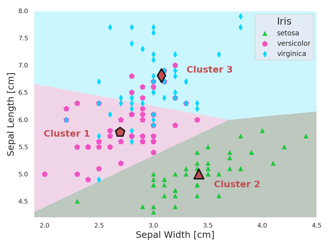
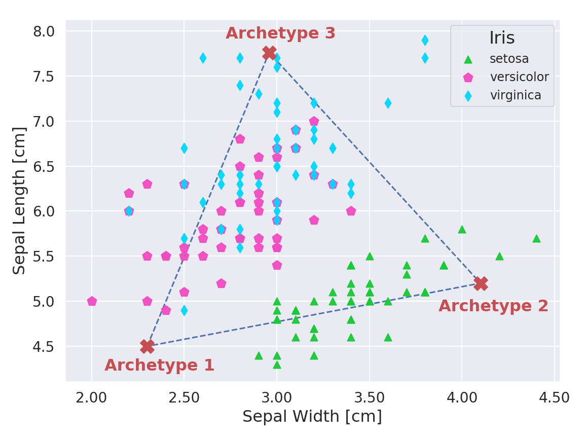
Colloquially, both the words “archetype” and “prototype” describe templates or original patterns from which all later forms are developed. However, the concept of a prototype is more common in machine learning and for example encountered as cluster-centroids in classification, where a query point is assigned to the class of the closest prototype. In an appropriate feature space such a prototype is a typical representative of its class, sharing all traits of the class members, ideally in equal proportion. By contrast, archetypes are characterized as being extreme points of the data, such that the complete data set can be well represented as a convex mixture of these extremes or archetypes. Archetypes thus form a polytope approximating the data convex hull. Based on the historic Iris flower data set (Anderson, 1935; Fisher, 1936), Figure 1 illustrates the different perspectives both approaches provide in exploring the data. In Figure 1(a) the cluster means as well as the decision boundaries in a 2-dimensional feature space are shown. The clustering was calculated using the k-Means algorithm. Each cluster mean is a typical average representative of its respective class, the aforementioned prototype. According to this clustering, the prototypical Iris virginica has a sepal width of 3.1cm and a sepal length of 6.8cm. On the other hand, Figure 1(b) shows the positions of the three archetypal Iris flowers, which are typical extreme representatives. The archetypal Iris virginica has a sepal width of 3.0cm and a sepal length of 7.8cm. All flowers within the simplex are characterized as weighted mixtures of these archetypes while, in terms of convex mixtures, the optimal location of flowers outside the simplex are normal projections onto its surface. In general, a clustering approach is more natural if the existence of a cluster structure can be presumed. Otherwise, archetypal analysis might offer an interesting perspective for exploratory data analysis.
2 Exploring Data Sets Through Archetypes
Archetypal analysis (AA) was first proposed by Cutler and Breiman (1994). It is a linear procedure where archetypes are selected by minimizing the squared error in representing each individual data point as a mixture of archetypes. Identifying the archetypes involves the minimization of a non-linear least squares loss.
2.1 Archetypal Analysis
Linear AA is a form of non-negative matrix factorization where a matrix of data vectors is approximated as with , , and usually . The so-called archetype matrix contains the archetypes with the model being subject to the following constraints:
| (1) |
Constraining the entries of and to be non-negative and demanding that both weight matrices are row stochastic implies a representation of the data vectors as a weighted sum of the rows of while simultaneously representing the archetypes themselves as a weighted sum of the data vectors in :
| (2) |
Due to the constraints on and in Eq. 1 both the representation of and in Eq. 2 are convex combinations. Therefore the archetypes approximate the data convex hull and increasing the number of archetypes improves this approximation. The central problem of AA is finding the weight matrices and for a given data matrix and a given number of archetypes. The non-linear optimization problem consists in minimizing the following residual sum of squares:
| (3) |
A probabilistic formulation of linear AA is provided by Seth and Eugster (2016) where it is observed that AA follows a simplex latent variable model and normal observation model. The generative process for the observations in the presence of archetypes with archetype weights is given by
| (4) |
with uniform concentration parameters for all , and weights summing up to . That is, the observations are distributed according to isotropic Gaussians with means and variance .
2.2 A Biological Motivation for Archetypal Analysis
Conceptionally, the motivation for Archetypal Analysis is purely statistical but the method itself always implied the possibility of interpretations with a more evolutionary flavour. By representing an individual data point as a mixture of pure types or archetypes, a natural link to the evolutionary development of biological systems is implicitly established. The publication by Shoval et al. (2012) entitled ’Evolutionary Trade-Offs, Pareto Optimality, and the Geometry of Phenotype Space’ made this connection explicit, providing a theoretical foundation of the ’archetype concept’. In general, evolutionary processes are multi-objective optimization problems and as such subject to unavoidable trade-offs: If multiple tasks need to be performed, no (biological) system can be optimal at all tasks at once. Examples of such trade-offs include those between longevity and fecundity in Drosophila melanogaster where long-lived flies show decreased fecundity (Djawdan et al., 1996) or predators that evolve to be fast runners but eventually have to trade-off their ability to subdue large or strong prey, e.g. cheetah versus lion (Garland, 2014). Such evolutionary trade-offs are known to affect the range of phenotypes found in nature (Tendler et al., 2015). In Shoval et al. (2012) it is argued that best-trade-off phenotypes are weighted averages of archetypes while archetypes themselves are phenotypes specialized at performing a single task optimally. An example of an evolutionary trade-off in the space of traits (or phenospace) for different species of bats (Microchiroptera) is shown in Figure 2. Based on a study of bat wings by Norberg et al. (1987), each species is represented in a two-dimensional space where the axis depict Body Mass and Wing Aspect Ratio. The latter is the square of the wingspan divided by the wing area.
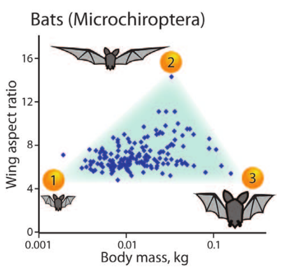
Table 1 gives an account of the task the archetypes indicated in Figure 2 have evolved to performing optimally. The trade-off situation can be interpreted using Pareto optimality theory (Steuer, 1986), which was recently used in biology to study trade-offs in evolution (Schuetz et al., 2012; El Samad et al., 2005). All phenotypes that have evolved over time lie within a restricted part of the phenospace, the so-called Pareto front, which is the set of phenotypes that cannot be improved at all tasks simultaneously. If there were a phenotype being better at all tasks than a second phenotype, then the latter would be eliminated over time by natural selection. Consequently phenotypes on the Pareto front are the best possible compromise between the different requirements or tasks.
| Archetype | Phenotype | Specialization |
|---|---|---|
| 1 | low aspect ratio, small body | hunting small insects near vegetation |
| 2 | high aspect ratio, medium body | hunting high flying large insects |
| 3 | low aspect ratio, large body | hunting animals near vegetation |
3 Related Work
Linear “Archetypal Analysis” (AA) was first proposed by Cutler and Breiman (1994). Since its conception, AA has known several advancements on the algorithmic side: In Stone and Cutler (1996) the authors propose an archetype model able to identify archetypes in space and time, named “archetypal analysis of spatio-temporal dynamics”. A similar problem is addressed in “Moving archetypes” by Cutler and Stone (1997). Model selection is the topic of Prabhakaran et al. (2012), where the authors are concerned with the optimal number of archetypes needed to characterize a given data set. An extension of the original archetypal analysis model to non-linear kernel archetypal analysis is proposed by Bauckhage and Manshaei (2014); Mørup and Hansen (2012). In Kaufmann et al. (2015), the authors use a copula based approach to make AA independent of strictly monotone transformations of the input data. The reasoning is that such transformations should in general not influence which points are identified as archetypes. Algorithmic improvements by adapting a Frank–Wolfe type algorithm to speed-up the calculation of archetypes are made by Bauckhage et al. (2015). A probabilistic version of archetypal analysis was introduced by Seth and Eugster (2016), lifting the restriction of archetypal analysis to real–valued data and instead allowing other observation types such as integers, binary, and probability vectors as input. Efficient “coresets for archetypal analysis” are proposed by Mair and Brefeld (2019) in order reduce the high computational cost due to the additional convexity-preserving constraints when identifying archetypes.
Although AA did not prevail as a commodity tool for pattern analysis, several applications have used it very successfully. In H. P. Chan et al. (2003), AA is used to analyse galaxy spectra which are viewed as weighted superpositions of the emissions from stellar populations, nebular emissions and nuclear activity. For the human genotype data studied by Huggins et al. (2007), inferred archetypes are interpreted as representative populations for the measured genotypes. In computer vision, AA has for example been used by Bauckhage and Thurau (2009) to find archetypal images in large image collections or by Canhasi and Kononenko (2015) to perform the analogous task for large document collections. In combination with deep learning, archetypal style analysis (Wynen et al., 2018) applies AA to learned image representations in order to realize artistic style manipulations.
Our work is based on the variational autoencoder model (VAE), arguably one of the most popular representatives of the class of “Deep Latent Variable Models”. VAEs were introduced by Kingma and Welling (2013); Rezende et al. (2014) and use an inference network to perform a variational approximation of the posterior distribution of the latent variables. Important work in this direction include Kingma et al. (2014); Rezende and Mohamed (2015) and Jang et al. (2017). More recently, Alemi et al. (2016) have discovered a close connection between VAE models and the Information Bottleneck principle (Tishby et al., 2000). Here, the Deep Variational Information Bottleneck (DVIB) is a VAE where not the input is reconstructed (i. e. decoded) but rather a datum , about which is known to contain information. Subsequently, the DVIB has been extended in multiple directions such as sparsity (Wieczorek et al., 2018) or causality (Parbhoo et al., 2018).
Akin to our work, AAnet is a model proposed by van Dijk et al. (2019) as an extension of linear archetypal analysis on the basis of standard, i. e. non-variational, autoencoders. In their work two regularization terms, applied to an intermediate representation, provide the latent archetypal convex representation of a non-linear transformation of the input. In contrast to our work, which is based on probabilistic generative models (VAE, DVIB), AAnet attempts to emulate the generative process by adding noise to the latent representation during training. Further, no side information is incorporated which can – and in our opinion should – be used to constrain potentially over-flexible neural networks and guide the optimisation process towards learning a meaningful representation.
4 Present Work
Archetypal analysis, as proposed by Cutler and Breiman (1994), is a linear method and cannot integrate any additional information about the data, e.g. labels, that might be available. Furthermore, the feature space in which AA is performed is spanned by features that had to be selected by the user based on prior knowledge. In the present work an extension of the original model is proposed such that appropriate representations can be learned end-to-end, side information can be incorporated to help learn these representations and non-linear relationships between features can be accounted for.
4.1 Deep Variational Information Bottleneck
We propose a model to generalise linear AA to the non-linear case based on the Deep Variational Information Bottleneck framework since it allows to incorporate side information by design and is known to be equivalent to the VAE in the case of , as shown in Alemi et al. (2016). In contrast to the data matrix in linear AA, a non-linear transformation giving rise to a latent representation of the data suitable for (non-linear) archetypal analysis is considered. I.e. the latent representation takes the role of the data in the previous treatment.
The DVIB combines the information bottleneck (IB) with the VAE approach (Tishby et al., 2000; Kingma and Welling, 2013). The objective of the IB method is to find a random variable which, while compressing a given random vector , preserves as much information about a second given random vector . The objective function of the IB is as follows
| (5) |
where is a Lagrange multiplier and denotes the mutual information. Assuming the IB Markov chain and a parametric form of Eq. 5 with parametric conditionals and , Eq. 5 is written as
| (6) |
As derived in Wieczorek et al. (2018), the two terms in Eq. 6 have the following forms:
| (7) | ||||
and
| (8) | ||||
Here denotes the entropy of in the discrete case or the differential entropy in the continuous case. The models in Eq. 7 and Eq. 8 can be viewed as the encoder and decoder, respectively. Assuming a standard prior of the form and a Gaussian distribution for the posterior , the KL divergence in Eq. 7 becomes a KL divergence between two Gaussian distributions which can be expressed in analytical form as in Kingma and Welling (2013). can then be estimated on mini-batches of size as
| (9) |
As for the decoder, in Eq. 8 is estimated using the reparametrisation trick proposed by Kingma and Welling (2013); Rezende et al. (2014):
| (10) | ||||
with the reparametrisation
| (11) |
As mentioned earlier, in the case of the original VAE is retrieved (Alemi et al., 2016). In our applications, we would like to predict not only the side information but also reconstruct the input . Similar to the approach proposed in Gomez-Bombarelli et al. (2018), we use an additional decoder branch to predict the reconstruction . This extension requires an additional term in the objective function Eq. 6 and an additional Lagrange multiplier . The mutual information estimate is obtained analogously to Eq. 10.
4.2 Deep Archetypal Analysis
Deep Archetypal Analysis can then be formulated in the following way. For the sampling of in Eq. 10 the probabilistic AA approach as in Eq. 4 can be used which leads to
| (12) |
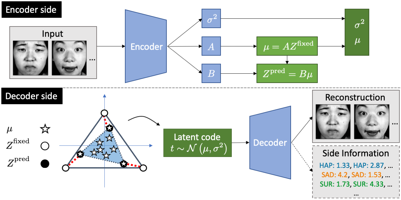
where the mean given through and variance are non-linear transformations of the data point learned by the encoder. We note that the means are convex combinations of weight vectors and the archetypes which in return are considered to be convex combinations of the means and weight vectors .111Note that (and not up to ), which reflects that deep neural networks usually require batch-wise training with batch size . By learning weight matrices and which are subject to the constraints formulated in Eq. 1 and parameterised by , a non-linear transformation of data is learned which drives the structure of the latent space to form archetypes whose convex combination yield the transformed data points. A major difference to linear AA is that for Deep AA we cannot identify the positions of the archetypes as there is no absolute frame of reference in latent space. We thus position archetypes at the vertex points of a -simplex and collect these fixed coordinates in the matrix . These requirements lead to an additional distance-dependent archetype loss of
| (13) |
where are the predicted archetype positions given the learned weight matrices and . For the loss function is minimized and the desired archetypal structure is achieved. The objective function of Deep AA is then given by
| (14) |
A visual illustration of Deep AA is given in Figure 3. The constraints on and can be guaranteed by using softmax layers and Deep AA can be trained with a standard stochastic gradient descent technique such as Adam (Kingma and Ba, 2014). Note that the model naturally allows to be relaxed to the VAE setting by omitting the side information term in Eq. 14.
4.3 The Necessity for Side Information
The goal of Deep AA is to identify meaningful archetypes in latent space which will subsequently allow the informed exploration of the given data set. The “meaning” of an archetype, and thereby the associated interpretation, can be improved by providing so-called side information, i.e. information in addition to the input data. If the input datum is for example an image, additional information could simply be a scalar- or vector-valued label. Using richer side information, e.g. additional images, is possible, too. The fundamental idea is that information about what constitutes a typical representative (in the archetypal sense) might not be information that is readily present in the input but dependent on – or even defined by – the side information. Taking a data set of car images as an example, what would be an archetypal car? Certainly, the overall size of a car would be a good candidate, such that smaller sports cars and larger pick-ups might be identified as archetypes. But introducing the fuel consumption of each car as side information would put sports cars and pick-ups closer together in latent space, as both car types often consume above average quantities of fuel. In this way, side information guides the learning of a latent representation which is informative with respect to exactly the side information provided. Consequently, typicality is not a characteristic of the data solely, but a function of the provided side information. And the selection of appropriate side information can only be linked to the question the user of a deep AA model tries to answer.
5 Experiments
5.1 Archetypal Analysis: Dealing With Non-linearity
Data generation.
For this experiment, data is generated that is a convex mixture of archetypes with . The generative process for the datum follows Eq. 4, where is a stochastic weight vector denoting the fraction of each of the archetypes needed to represent the data point . A total of data points is generated, of which are true archetypes. The variance is set to and the linear 3-dim data manifold is embedded in a dimensional space. Note that although linear and deep archetypal analysis is always performed on the full data set, only a fraction of that data is displayed when visualizing results.
Linear AA – non-linear data.
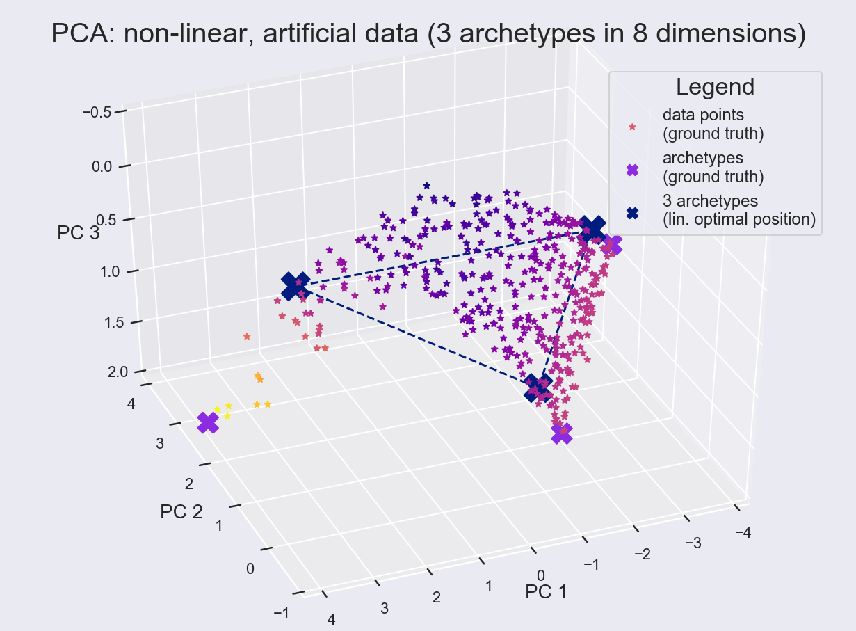
Data is generated as described above and an additional non-linearity is introduced by applying an exponential to one dimension of which results in a curved 8-dimensional data manifold. Linear archetypal analysis is then performed using the efficient Frank-Wolfe procedure proposed by Bauckhage et al. (2015). For visualization, PCA is used to recover the original 3-dimensional data submanifold which is embedded in the 8-dimensional space. The first three principal components of the ground truth data are shown in Figure 4(a) as well as the computed archetypes (connected by dashed lines). The positions of the computed archetypes occupy optimal positions according to the optimization problem in equation 3 but due to the non-linearity in the data it is impossible to recover the three ground truth archetypes.
Deep AA – non-linear data.
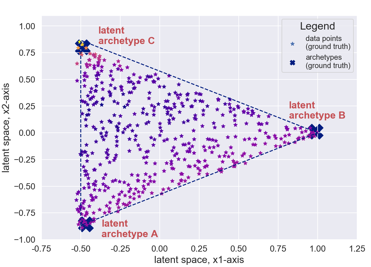
For data that has been generated as described in the previous paragraph, a strictly monotone transformation in form of an exponentiation should in general not change which data points are identified as archetypes. But this is clearly the case for linear AA as it is unable to recover the true archetypes after a non-linearity has been applied. Using that same data to train the deep AA architecture presented in Figure 3 generates the latent space structure shown in Figure 4(b), where the three archetypes A, B and C have been assigned to the appropriate vertices of the latent simplex. Moreover, the sequence of color stripes shown has been correctly mapped into the latent space. Within the latent space data points are again described as convex linear combinations of the latent archetypes. Latent data points can also be reconstructed in the original data space through the learned decoder network. The network architecture used for this experiment was a simple feedforward network (2 layered encoder and decoder), training for 20 epochs with a batch size of 100 and a learning rate of 0.001.
5.2 Archetypes in Image-based Sentiment Analysis
The Japanese Female Facial Expression (JAFFE) database was introduced by Lyons et al. (1998) and contains 213 images of 7 facial expressions (6 basic facial expressions + 1 neutral). The expressions are happiness, sadness, surprise, anger, disgust and fear. All expressions were posed by 10 Japanese female models. Each image has been rated on 6 emotion adjectives by 60 Japanese subjects on a 5 level scale (5-high, 1-low) and each image was then assigned a 6-dim. vector of average ratings. For the following experiments the advice of the creator of the JAFFE data set was followed to exclude fear images and the fear adjective from the ratings, as the models were not believed to be good at posing fear. All experiments based on the JAFFE data set are performed on the following architecture222The code is available via https://github.com/bmda-unibas/DeepArchetypeAnalysis:
- •
-
Encoder:
Input: image (128128)
3[64 Conv. (44) + Max-Pool. (22)]
Flatten + FC100
, , - •
-
Decoder (Image Branch):
Input: latent code
FC49
3[64 Conv. Transpose (44)]
Flatten + FC128128
FC128128 128128 reconstruction - •
-
Decoder (Side Information Branch):
Input: latent code
FC200-5 side information
ReLU activations are used in-between layers and sigmoid activations for the image intensities. The different losses are weighted as follows: we multiplied the archetype loss by a factor of 80, the side information loss by 560, and the KL divergence by 40. In the setting where only two labels are considered, the weight for archetype loss is increased to 120. The network was trained for 5000 epochs with a mini-batch size of 50 and a learning rate of 0.0001. For training a NVIDIA TITAN X Pascal GPU was used, where a full training sessions lasted approximately 30 minutes.
5.2.1 JAFFE: Latent Space Structure
Emotions conveyed through facial expressions are a suitable case to demonstrate the interpretability of learned latent representation in deep AA. First, the existence of archetypes is plausible as there clearly are expressions that convey a maximum of a given emotion, i. e. a person can look extremely/maximally surprised.
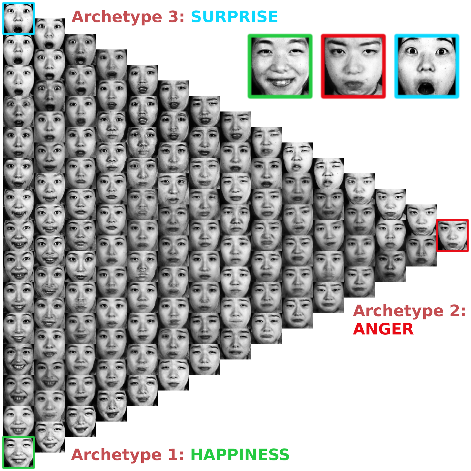
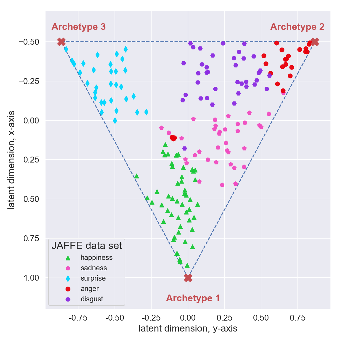
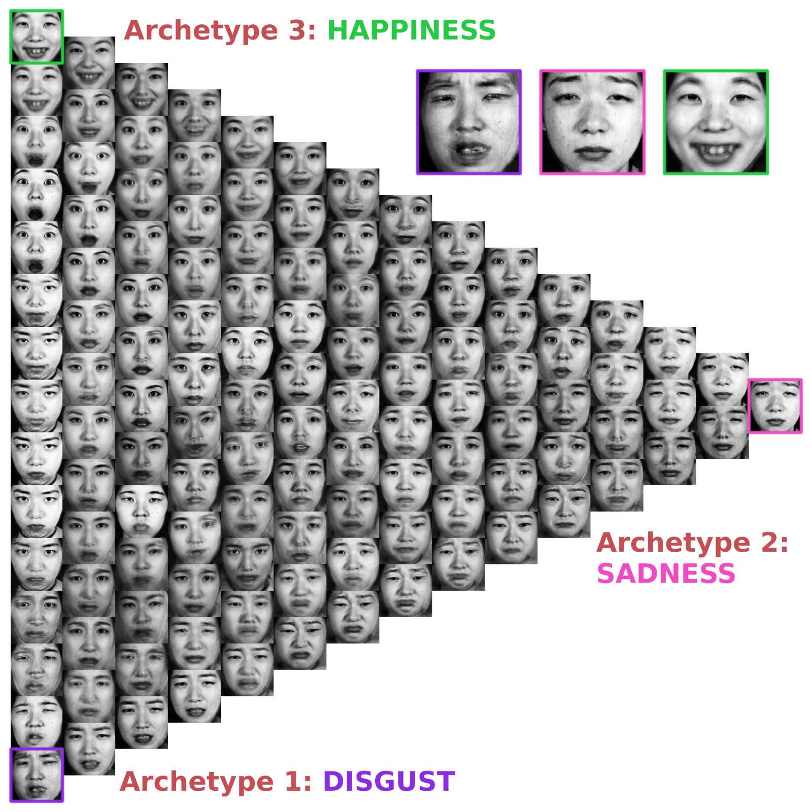
Second, facial expressions change continuously without having a clearly defined cluster structure. Moreover, these expressions lend themselves to being interpreted as mixtures of basic (or archetypal) emotional expressions – a perspective also enforced by the averaged ratings for each image which are essentially weight vectors with respect to the archetypal emotional expressions. Figure 5(a) shows the learned archetypes “happiness”, “anger” and “surprise” while expressions linked to the emotion adjective “sadness” are identified as mixtures between archetype 1 (happiness) and archetype 2 (anger). Figure 5(b) shows the positions of the latent means where the color coding is based on the argmax of the emotion rating, which is a 5-dimensional vector. An analogous situation is found in case of “disgust”, which, according to deep AA, is a mixture between archetype 2 (anger) and archetype 3 (surprise). Towards the center of the simplex, expressions are located which share equal weights with respect to the archetypes and thus resemble a more “neutral” facial expression, as shown in figure 8.
Side Information for JAFFE.
The JAFFE data set contains facial expressions posed by 10 Japanese female models. Based solely on the visual information, i.e. disregarding the emotion scores, these images could meaningfully be grouped together in a variety of ways, e. g. head shape, hair style, identity of the model posing the expressions… Interpreting resulting archetypes in general requires guiding information that tells the model which “definition of typicality” it is required to learn. While it is obvious to learn typical emotion expressions in case of JAFFE, most applications are arguably more ambiguous. In section 5.3 a chemical experiment is discussed, where each molecule can be described by a variety of properties. The side information introduced to the learning process will ultimately be the property the experimenter is interested in, and typicality will have to be understood with respect to that property.
5.2.2 JAFFE: Expressions As Weighted Mixtures
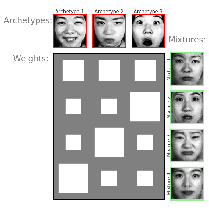
One advantage of deep AA compared to the plain Variational Autoencoder (VAE) is a globally interpretable latent structure. All latent means will be mapped inside the convex region spanned by the archetypes. And as archetypes represent extremes of the data set which are present to some percentage in all data points, these percentages or weights can be used to explore the latent space in an informed fashion. This might be especially of advantage in case of higher-dimensional latent spaces. For example will the center of the simplex always accommodate latent representations of input data that are considered mean samples of the data set. Moreover, directions within the simplex have meaning in the sense that when “walking” towards or away from a given archetype, the characteristics of that archetype will either be enforce or diminished in the decoded datum associated with the actual latent position. This is shown in the Hinton plot in Figure 6 where mixture 1 is a mean sample, i. e. with equal archetype weights. Starting at this position and moving on a straight line into the direction of archetype 3 increases its influence while equally diminishing the influence of both archetypes 1 and 2. This results in mixture 2 which starts to look surprised, but not as extremely surprised as archetype 3. In the same fashion mixture 3 and 4 are the results of walking straight into the direction of archetypes 2 or 1 which results in a sad face (mixture 3) and a slightly happy facial expression (mixture 4).
5.2.3 JAFFE: Deep AA Versus VAE
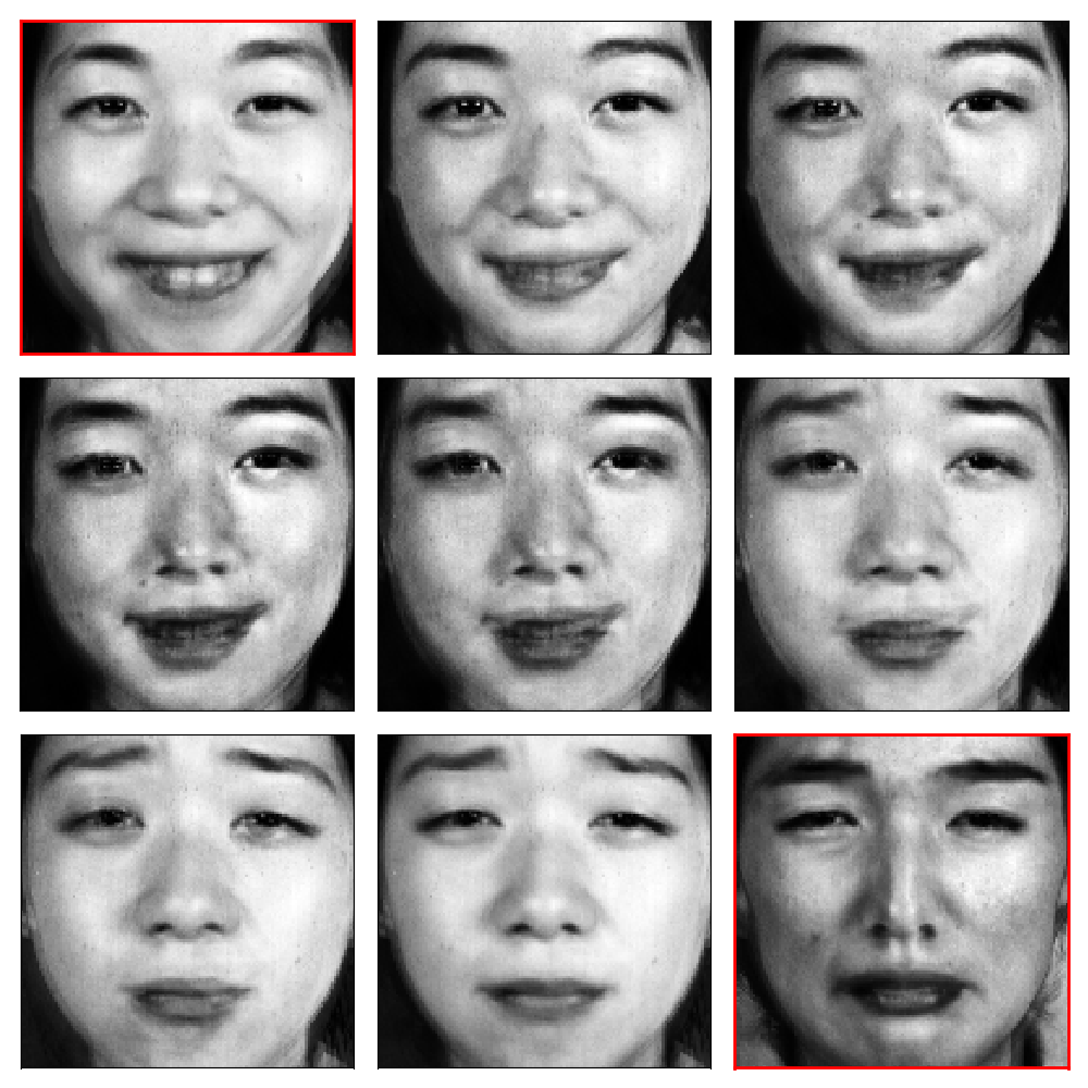
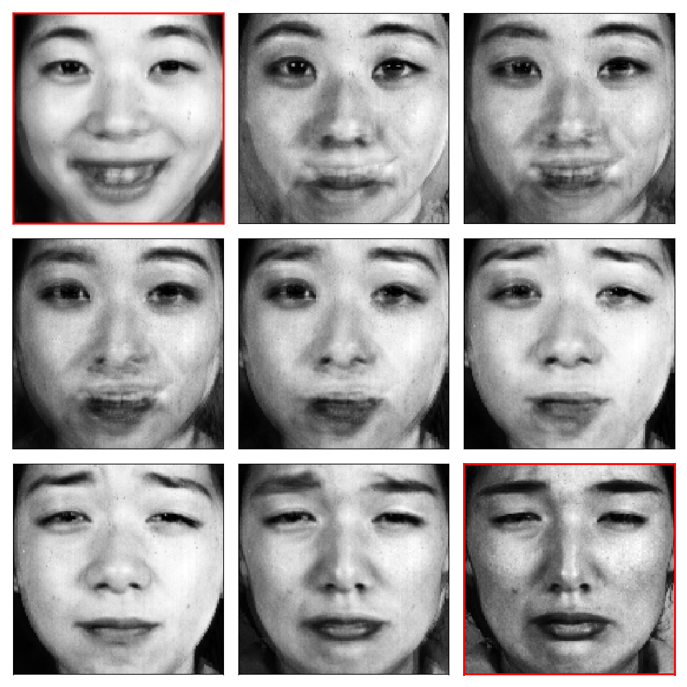
Deep AA is designed to be a model that simultaneously learns an appropriate representation and identifies meaningful latent archetypes. This model can be compared to a plain VAE where a latent space is learned first and subsequently linear AA is performed on that space in order to approximate the latent convex hull. Figure 7(a) shows the interpolation in the deep AA model between two images, neither of them archetypes, from “happy” to “sad”. Compared to Figure 7(b), which shows the same interpolation in a VAE model with subsequently performed linear AA, the interpolation based on deep AA gives a markedly better visual impression. In case of deep AA, this is explained by the fact that all data points are mapped into the simplex which ensures a relatively dense distribution of the latent means. On the other hand, the latent space of the VAE model has no hard geometrical restrictions and thus the distribution of the latent representatives will be less dense or even “patchy”, i. e. with larger empty areas in latent space. Especially with small data sets such as JAFFE, of which less than 200 images are used, interpolation quality might be strongly affected by the unboundedness of the latent space of VAE models.
5.3 The Chemical Universe Of Molecules
In the following section the application of deep AA to the domain of chemistry is explored. Starting with an initial set of chemical compounds, e. g. small organic molecules with cyclic cores (Visini et al., 2017), and iteratively applying a finite number of reactions, will eventually lead to a huge collection of molecules with extreme combinatorial complexity. But while the total number of all possible small organic molecules has been estimated to exceed (Kirkpatrick and Ellis, 2004), even this number pales in comparison to the whole chemical universe of organic chemistry. In general, the efficient exploration of chemical spaces requires methods capable of learning meaningful representations and endowing these spaces with a globally interpretable structure. Prominent examples of chemistry data sets include the family of GDB-xx data sets (generic database), e. g. GDB-13 (Blum and Reymond, 2009), which enumerates small organic molecules of up to 13 atoms, composed of the elements C, N, O, S and Cl, following simple chemical stability and synthetic feasibility rules. With more than 970 million structures, GDB-13 is the largest publicly available database of small organic molecule to date.
Exploring The Chemical Space.
As discussed in section 2.2, archetypal analysis lends itself to a distinctly evolutionary interpretation. Although this is certainly a more biological perspective, the basic principle is applicable to other fields. In chemistry, the principle of evolutive abiogenesis describes a process in which simple organic compounds increase in complexity (Miller, 1953). In the following experiment a structured chemical space is learned using as side information the heat capacity which quantifies the amount of energy (in Joule) needed to increase 1 Mol of molecules by 1 K at constant volume. A high number is important e. g. in applications dealing with the storage of thermal energy (Cabeza et al., 2015). In the following, all experiments are based on the QM9 data set (Ramakrishnan et al., 2014; Ruddigkeit et al., 2012), which contains molecular structures and properties of 134k organic molecules. Each molecule is made up of nine or less atoms, i. e. C, O, N, or F, without counting hydrogen. The QM9 data set is based on ab-initio density functional theory (DFT) calculations.

Experiment Setup.
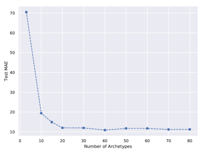
A total of 204 features were extracted for every molecule using the Chemistry Development Kit (Steinbeck et al., 2003). The neural architecture used has 3 hidden FC layers with 1024, 512 and 256 neurons, respectively and ReLU activation functions. For all experiments, the model was trained in a supervised fashion by reconstructing the molecules and the side information simultaneously. In Experiment 1, model selection was performed by continuously increasing the number of latent dimensions. Based on the knee of the mean absolute error (MAE), the appropriate number of latent archetypes was selected. In Experiments 2 and 3, the number of latent dimensions was fixed to 19, corresponding to the optimal number of 20 archetypes from the model selection procedure. During training, the Lagrange multiplier was steadily increased by increments of 1.01 every 500 iterations. For training, the Adam optimizer (Kingma and Ba, 2014) was used, with an initial learning rate of 0.01. A learning rate decay was introduced, with an exponential decay of 0.95 every 10k iterations. The batch size was 2048 and the model was trained for a total of 350k iterations. The data set is divided in training and test set with a 90%/10% split. For visualization, the 3-dimensional molecular representations haven been created with Jmol (2019).
Experiment 1: Model Selection.
MAE error is assessed while varying the number of archetypes. The result is shown in Figure 9. Model selection is performed by observing for which number of archetypes the MAE starts to converge. The knee of this curve is used to select the optimal number of archetypes, which is 20. Obviously, if the number of archetypes is smaller, it becomes more difficult to reconstruct the data. This is explained by the fact that there exists a large number of molecules with very similar heat capacities but at the same time distinctly different geometric configurations. As a consequence, molecules with different configurations are mapped to archetypes with the similar heat capacity, making it hard to resolve the many–to–one mapping in the latent space.
Experiment 2: Archetypal Molecules.
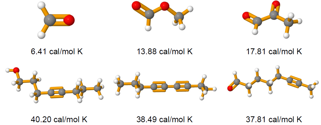
Archetypal molecules are identified along with the heat capacities associated with them. A fixed number of 20 archetypes is used for optimal exploration-exploitation trade-off, in accordance with the model selection discussed in the previous section. In chemistry, the heat capacity at constant volume is defined as where denotes the energy of a molecule and its temperature. This energy can be further decomposed into different parts, such that . Each part is associated with a different degree of freedom of the system. Here, stands for translational, for rotational, for vibrational and for the electronic contributions to the total energy of the system (Atkins and de Paula, 2010; Tinoco, 2002). With this decomposition in mind, the different archetypal molecules associated with a particular heat capacity are compared in Figure 10. In both panels of that figure, the rows correspond to the three molecules in the QM9 data set (test set) that have been mapped closest to a vertex of the latent simplex and have thus been identified as being extremes with respect to the heat capacity. Out of a total of 20 vertices, molecules in close proximity to four of them are displayed here. Panel 10(a) shows the configuration of six archetypal molecules. The upper three are all associated with a low heat capacity while the lower three all have a high heat capacity. This result can easily be interpreted, as the lower heat capacity can be traced back to the shorter chain length and the higher number of double bonds of these molecules, which makes them more stable and results in a lower vibrational energy and subsequently in a lower heat capacity. The inverse is observed for the linear archetypal molecules with higher heat capacities, which show, relative to their size, a lower number of double bonds and a long linear structure. Panel 10(b) shows both linear (lower row) and non-linear archetypal molecules (upper row) but with similar atomic mass. Here, the non-linear molecules containing a cyclic structure in their geometry, are more stable and therefore have an overall slightly lower heat capacity compared to their linear counterparts of the same weight, shown in the second row.
Experiment 3: Interpolation Between Two Archetypal Molecules.
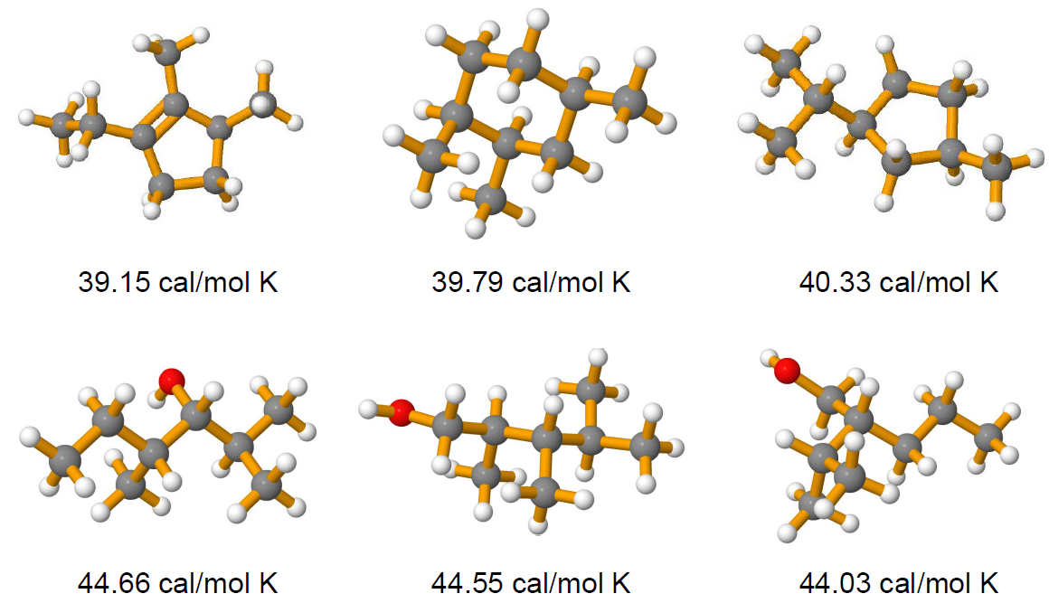
Interpolation is performed by plotting the samples from the test set which are closest to the connecting line between the two archetypes. As a result, one can observe a smooth transition from a molecule with a ring structure to a linear chain molecule. Both the starting and the end point of this interpolation is characterized by a similar heat capacity, such that these archetypes differ only in their geometric configuration but not with respect to their side information. As a consequence, any molecule in close proximity to that connecting line can differ only with respect to its structure, but must display a similarly high heat capacity. Figure 11 shows an example of such an interpolation.
Experiment 4: The Role Of Side Information And The Exploration Of Chemical Space.
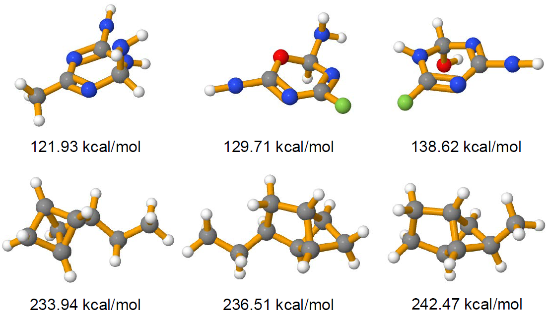
Deep AA structures latent spaces both according to the information contained in the input to the encoder as well as the side information provided. As a consequence, any molecule characterized as a true mixture of two or more archetypes, given a specific side information such as heat capacity, might suddenly be identified as archetypal should the side information change accordingly. In the following, archetypal molecules with respect to heat capacity as the side information are compared to archetypes obtained while providing the band gap energy of each molecule as the side information. In Figure 12(a) archetypal molecules with both the highest and the lowest heat capacities are displayed while 12(b) shows archetypes with highest and lowest band gap energies. The archetypes significantly differ in their structure as well as their atomic composition. For example, archetypal molecules with low heat capacity are rather small, with only few C and O atoms, while archetypal molecules with a low band gap energy are characterized by ring structures containing N and H atoms. This illustrates how essential side information is for defining typicality but also for the subsequent interpretation of the obtained structure of the latent space.

5.4 Alternative Priors For Deep Archetypal Analysis
The standard normal distribution is a typical choice for the prior distribution due to its simplicity and closed form solutions for the KL divergence. However, employing alternative priors might be beneficial for the structure of the latent space and have an impact on the identified archetypes.
Leaving the wide range of well explored priors for vanilla VAEs aside, we explore a hierarchical prior that directly corresponds to the generative model of linear AA (Eq. 4), i.e. isotropic Gaussian noise around a linear combination of the archetypes:
| (15) |
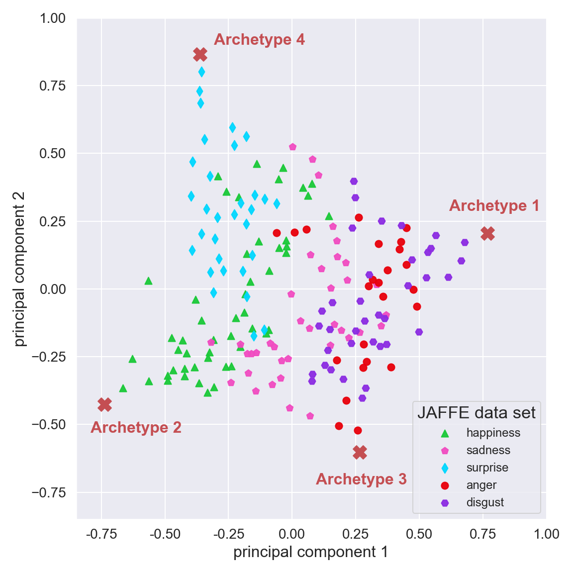
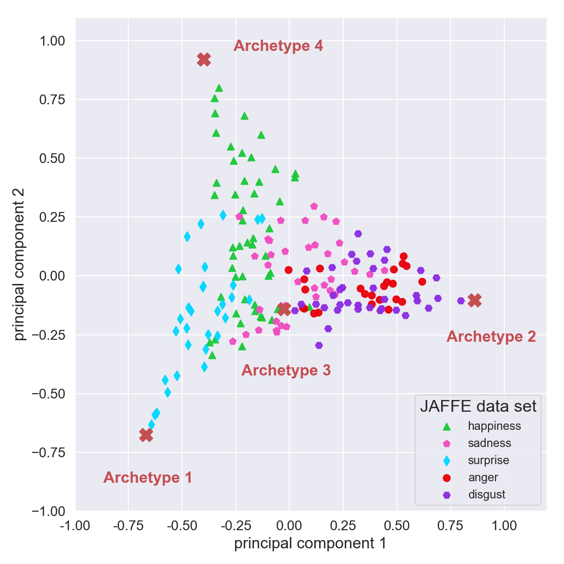
We rely on Monte-Carlo sampling for the estimation of the KL divergence in Eq. 7. For comparing the different priors qualitatively, we run Deep AA on the Japanese Face Expressions with four archetypes. The architecture used is similar to the previous experiments but we additionally learn the variance of the decoder. The Lagrange parameters or weights in Eq. 14 are set to 1000 for the archetype loss and to 100 for the KL divergence.
Figure 13 shows examples of the found archetypes for the standard normal prior and the sampling Dirichlet prior. In general, different priors do not seem to strongly affect the found archetypes. However, the latent spaces do differ, which can be seen in the projection to the first two principal components in Figure 14. As a reference, a uniformly filled simplex would result in a triangle in the projection. The difference is caused by large gaps in the higher-dimensional simplex when using the hierarchical prior, which we assume is mainly due to the high variance estimation of the KL divergence.
In our experience, the choice of the prior is not of primary concern for finding archetypes, as long as it encourages the latent space to be spread out inside the simplex – be that via a standard normal, a uniform or the presented hierarchical prior.


6 Conclusion
We have presented in this paper an extension of linear Archetypal Analysis, a technique for exploratory data analysis and interpretable machine learning. By performing Archetypal Analysis in the latent space of a Variational Autoencoder, we have demonstrated that the learned representation can be structured in a way that allows it to be characterized by its most extremal or archetypal representatives. As a result, each observation in a data set can be described as a convex mixture of these extremes. Endowed with such a structure, a latent space can be explored by varying the mixture coefficients with respect to the archetypes, instead of exploring the space by uniform sampling. Furthermore, we have demonstrated the need for including side information into the process of learning latent archetypal representations. As extremity is a form of typicality, a definition of what is understood to be “typical” needs to be given first. Providing such a definition is the role of side information and allows learning interpretable archetypes. In contrast to the original archetype model, our method offers three advantages: First, our model learns representations in a data-driven fashion, thereby reducing the need for expert knowledge. Second, our model can learn appropriate transformations to obtain meaningful archetypes, even if non-linear relations between features exist. Third, the incorporation of side information. The application of this new method is demonstrated on a sentiment analysis task, where emotion archetypes are identified based on female facial expressions, for which multi-rater based emotion scores are available as side information. A second application illustrates the exploration of the chemical space of small organic molecules and demonstrated how crucial side information is for interpreting the geometric configuration of these molecules.
References
- Alemi et al. (2016) Alemi AA, Fischer I, Dillon JV, Murphy K (2016) Deep variational information bottleneck. CoRR abs/1612.00410, URL http://arxiv.org/abs/1612.00410, 1612.00410
- Anderson (1935) Anderson E (1935) The irises of the gaspe peninsula. Bulletin of the American Iris Society 59:2–5
- Atkins and de Paula (2010) Atkins P, de Paula J (2010) Atkins’ Physical Chemistry. OUP Oxford
- Bauckhage and Manshaei (2014) Bauckhage C, Manshaei K (2014) Kernel archetypal analysis for clustering web search frequency time series. In: 2014 22nd International Conference on Pattern Recognition, pp 1544–1549, DOI 10.1109/ICPR.2014.274
- Bauckhage and Thurau (2009) Bauckhage C, Thurau C (2009) Making archetypal analysis practical. In: Denzler J, Notni G, Süße H (eds) Pattern Recognition, Springer Berlin Heidelberg, pp 272–281
- Bauckhage et al. (2015) Bauckhage C, Kersting K, Hoppe F, Thurau C (2015) Archetypal analysis as an autoencoder. In: Workshop New Challenges in Neural Computation 2015, pp 8–16, URL https://www.techfak.uni-bielefeld.de/~fschleif/mlr/mlr\_03\_2015.pdf
- Blum and Reymond (2009) Blum LC, Reymond JL (2009) 970 million druglike small molecules for virtual screening in the chemical universe database gdb-13. Journal of the American Chemical Society 131(25):8732–8733, DOI 10.1021/ja902302h, pMID: 19505099
- Cabeza et al. (2015) Cabeza LF, Gutierrez A, Barreneche C, Ushak S, Fernandez AG, Fernadez AI, Grageda M (2015) Lithium in thermal energy storage: A state-of-the-art review. Renewable and Sustainable Energy Reviews 42:1106 – 1112
- Canhasi and Kononenko (2015) Canhasi E, Kononenko I (2015) Weighted hierarchical archetypal analysis for multi-document summarization. Computer Speech & Language 37, DOI 10.1016/j.csl.2015.11.004
- Cutler and Breiman (1994) Cutler A, Breiman L (1994) Archetypal analysis. Technometrics 36(4):338–347, DOI 10.1080/00401706.1994.10485840, URL http://digitalassets.lib.berkeley.edu/sdtr/ucb/text/379.pdf
- Cutler and Stone (1997) Cutler A, Stone E (1997) Moving archetypes. Physica D: Nonlinear Phenomena 107(1):1–16, DOI 10.1016/s0167-2789(97)84209-1, URL https://doi.org/10.1016/s0167-2789(97)84209-1
- van Dijk et al. (2019) van Dijk D, Burkhardt D, Amodio M, Tong A, Wolf G, Krishnaswamy S (2019) Finding archetypal spaces for data using neural networks. arXiv preprint arXiv:190109078
- Djawdan et al. (1996) Djawdan M, Sugiyama TT, Schlaeger LK, Bradley TJ, Rose MR (1996) Metabolic aspects of the trade-off between fecundity and longevity in drosophila melanogaster. Physiological Zoology 69(5):1176–1195
- El Samad et al. (2005) El Samad H, Khammash M, Homescu C, Petzold L (2005) Optimal performance of the heat-shock gene regulatory network. Proceedings 16th IFAC World Congress 16, URL https://engineering.ucsb.edu/~cse/Files/IFACC\_HS\_OPT04.pdf
- Fisher (1936) Fisher RA (1936) The use of multiple measurements in taxonomic problems. Annals of Eugenics 7(Part II):179–188
- Garland (2014) Garland TJJ (2014) Quick guides: Trade-offs. Current Biology 24(2):R60–R61
- Gomez-Bombarelli et al. (2018) Gomez-Bombarelli R, Wei JN, Duvenaud D, Hernández-Lobato JM, Sánchez-Lengeling B, Sheberla D, Aguilera-Iparraguirre J, Hirzel TD, Adams RP, Aspuru-Guzik A (2018) Automatic chemical design using a data-driven continuous representation of molecules. ACS Central Science 4(2):268–276
- H. P. Chan et al. (2003) H P Chan B, Mitchell D, Cram L (2003) Archetypal analysis of galaxy spectra. Monthly Notices of the Royal Astronomical Society 338, DOI 10.1046/j.1365-8711.2003.06099.x
- Huggins et al. (2007) Huggins P, Pachter L, Sturmfels B (2007) Toward the human genotope. Bulletin of Mathematical Biology 69(8):2723–2735, DOI 10.1007/s11538-007-9244-7, URL https://doi.org/10.1007/s11538-007-9244-7
- Jang et al. (2017) Jang E, Gu S, Poole B (2017) Categorical Reparameterization with Gumbel-Softmax. International Conference on Learning Representations (ICLR)
- Jmol (2019) Jmol (2019) Jmol: an open-source java viewer for chemical structures in 3d URL http://www.jmol.org/
- Kaufmann et al. (2015) Kaufmann D, Keller S, Roth V (2015) Copula archetypal analysis. In: Gall J, Gehler P, Leibe B (eds) Pattern Recognition, Springer International Publishing, pp 117–128
- Kingma and Ba (2014) Kingma DP, Ba J (2014) Adam: A method for stochastic optimization. abs/1412.6980
- Kingma and Welling (2013) Kingma DP, Welling M (2013) Auto-encoding variational bayes. CoRR abs/1312.6114
- Kingma et al. (2014) Kingma DP, Mohamed S, Rezende DJ, Welling M (2014) Semi-supervised learning with deep generative models. In: Advances in Neural Information Processing Systems 27: Annual Conference on Neural Information Processing Systems 2014, December 8-13 2014, Montreal, Quebec, Canada, pp 3581–3589
- Kirkpatrick and Ellis (2004) Kirkpatrick P, Ellis C (2004) Chemical space. Nature 432(823):1476–4687, DOI 10.1038/432823a
- Lyons et al. (1998) Lyons MJ, Akamatsu S, Kamachi M, Gyoba J (1998) Coding facial expressions with gabor wavelets. 3rd IEEE International Conference on Automatic Face and Gesture Recognition pp 200–205, DOI 10.1109/AFGR.1998.670949, URL https://zenodo.org/record/3430156
- Mair and Brefeld (2019) Mair S, Brefeld U (2019) Coresets for archetypal analysis. In: Advances in Neural Information Processing Systems 32, Curran Associates, Inc., pp 7245–7253, URL http://papers.nips.cc/paper/8945-coresets-for-archetypal-analysis.pdf
- Miller (1953) Miller SL (1953) A production of amino acids under possible primitive earth conditions. Science pp 528–529
- Mørup and Hansen (2012) Mørup M, Hansen LK (2012) Archetypal analysis for machine learning and data mining. Neurocomputing 80:54–63
- Norberg et al. (1987) Norberg UM, Rayner JMV, Lighthill MJ (1987) Ecological morphology and flight in bats (mammalia; chiroptera): wing adaptations, flight performance, foraging strategy and echolocation. Philosophical Transactions of the Royal Society of London B, Biological Sciences 316(1179), URL https://royalsocietypublishing.org/doi/abs/10.1098/rstb.1987.0030
- Parbhoo et al. (2018) Parbhoo S, Wieser M, Roth V (2018) Causal Deep Information Bottleneck. arXiv e-prints arXiv:1807.02326, 1807.02326
- Prabhakaran et al. (2012) Prabhakaran S, Raman S, Vogt JE, Roth V (2012) Automatic model selection in archetype analysis. In: Pinz A, Pock T, Bischof H, Leberl F (eds) Pattern Recognition, Springer Berlin Heidelberg, pp 458–467
- Ramakrishnan et al. (2014) Ramakrishnan R, Dral PO, Rupp M, von Lilienfeld OA (2014) Quantum chemistry structures and properties of 134 kilo molecules. Scientific Data 1
- Rezende and Mohamed (2015) Rezende D, Mohamed S (2015) Variational inference with normalizing flows. In: Bach F, Blei D (eds) Proceedings of the 32nd International Conference on Machine Learning, PMLR, Lille, France, Proceedings of Machine Learning Research, vol 37, pp 1530–1538
- Rezende et al. (2014) Rezende DJ, Mohamed S, Wierstra D (2014) Stochastic backpropagation and approximate inference in deep generative models 32(2):1278–1286
- Ruddigkeit et al. (2012) Ruddigkeit L, van Deursen R, Blum LC, Reymond JL (2012) Enumeration of 166 billion organic small molecules in the chemical universe database gdb-17. Journal of Chemical Information and Modeling 52(11):2864–2875, DOI 10.1021/ci300415d, URL https://pubs.acs.org/doi/10.1021/ci300415d, pMID: 23088335
- Schuetz et al. (2012) Schuetz R, Zamboni N, Zampieri M, Heinemann M, Sauer U (2012) Multidimensional optimality of microbial metabolism. Science (New York, NY) 336:601–4, DOI 10.1126/science.1216882
- Seth and Eugster (2016) Seth S, Eugster MJA (2016) Probabilistic archetypal analysis. Machine Learning 102(1):85–113, DOI 10.1007/s10994-015-5498-8, URL https://doi.org/10.1007/s10994-015-5498-8
- Shoval et al. (2012) Shoval O, Sheftel H, Shinar G, Hart Y, Ramote O, Mayo A, Dekel E, Kavanagh K, Alon U (2012) Evolutionary trade-offs, pareto optimality, and the geometry of phenotype space. Science 336(6085):1157–1160, DOI 10.1126/science.1217405, URL http://science.sciencemag.org/content/336/6085/1157, http://science.sciencemag.org/content/336/6085/1157.full.pdf
- Steinbeck et al. (2003) Steinbeck C, Han YQ, Kuhn S, Horlacher O, Luttmann E, Willighagen E (2003) The Chemistry Development Kit (CDK): An open-source Java library for chemo- and bioinformatics. Journal of Chemical Information and Computer Sciences 43(2):493–500
- Steuer (1986) Steuer R (1986) Multiple Criteria Optimization: Theory, Computation and Application. John Wiley & Sons
- Stone and Cutler (1996) Stone E, Cutler A (1996) Introduction to archetypal analysis of spatio-temporal dynamics. Physica D: Nonlinear Phenomena 96(1-4):110–131, DOI 10.1016/0167-2789(96)00016-4, URL https://doi.org/10.1016/0167-2789(96)00016-4
- Tendler et al. (2015) Tendler A, Mayo A, Alon U (2015) Evolutionary tradeoffs, pareto optimality and the morphology of ammonite shells. BMC Systems Biology 9(1), DOI 10.1186/s12918-015-0149-z, URL https://doi.org/10.1186/s12918-015-0149-z
- Tinoco (2002) Tinoco I (2002) Physical Chemistry: Principles and Applications in Biological Sciences. No. S. 229-313 in Physical Chemistry: Principles and Applications in Biological Sciences, Prentice Hall
- Tishby et al. (2000) Tishby N, Pereira FC, Bialek W (2000) The information bottleneck method. arXiv preprint physics/0004057
- Visini et al. (2017) Visini R, Arus-Pous J, Awale M, Reymond JL (2017) Virtual exploration of the ring systems chemical universe. Journal of Chemical Information and Modeling 57(11):2707–2718, DOI 10.1021/acs.jcim.7b00457, URL https://doi.org/10.1021/acs.jcim.7b00457, pMID: 29019686, https://doi.org/10.1021/acs.jcim.7b00457
- Wieczorek et al. (2018) Wieczorek A, Wieser M, Murezzan D, Roth V (2018) Learning Sparse Latent Representations with the Deep Copula Information Bottleneck. International Conference on Learning Representations (ICLR)
- Wynen et al. (2018) Wynen D, Schmid C, Mairal J (2018) Unsupervised learning of artistic styles with archetypal style analysis. In: Advances in Neural Information Processing Systems, pp 6584–6593