Data-Driven Discovery of Coarse-Grained Equations

Abstract

Statistical (machine learning) tools for equation discovery require large amounts of data that are typically computer generated rather than experimentally observed. Multiscale modeling and stochastic simulations are two areas where learning on simulated data can lead to such discovery. In both, the data are generated with a reliable but impractical model, e.g., molecular dynamics simulations, while a model on the scale of interest is uncertain, requiring phenomenological constitutive relations and ad-hoc approximations. We replace the human discovery of such models, which typically involves spatial/stochastic averaging or coarse-graining, with a machine-learning strategy based on sparse regression that can be executed in two modes. The first, direct equation-learning, discovers a differential operator from the whole dictionary. The second, constrained equation-learning, discovers only those terms in the differential operator that need to be discovered, i.e., learns closure approximations. We illustrate our approach by learning a deterministic equation that governs the spatiotemporal evolution of the probability density function of a system state whose dynamics are described by a nonlinear partial differential equation with random inputs. A series of examples demonstrates the accuracy, robustness, and limitations of our approach to equation discovery.

1 Introduction

Empiricism, or the use of data to discern fundamental laws of nature, lies at the heart of the scientific method. With the advent of “machine learning”, this ancient facet of pursuit of knowledge takes the form of inference, from observational or simulated data, of either analytical relations between inputs and outputs [24] or governing equations for system states [11, 16, 18, 19, 27, 36]. The advantage of learning a governing equation, rather than an input-output map for a quantity of interest (QoI), is the possibility to “generalize” (extrapolate) over space and time and over different external inputs such as initial and boundary conditions. In this sense, learning a differential equation is akin to learning an iterative algorithm that generates a solution, rather than learning the solution itself. Of direct relevance to the present study is the use of sparse regression on noisy data to estimate the constant coefficients in nonlinear ordinary [8] and partial [22, 23] differential equations (ODEs and PDEs, respectively). This strategy has been generalized to recover variable coefficients [21] or nonlinear constitutive relations between several state variables [28].

In physical sciences, observational data are seldom, if ever, sufficient to accomplish this goal; instead, the data must be generated by solving a governing equation. This strategy provides a partial explanation for why machine learning methods are yet to discover new physical laws: to generate the data one needs to know the underlying equation, which is subsequently learned from these data. Multiscale modeling and stochastic simulations are two areas where learning on simulated data can lead to real discovery. In multiscale simulations, one is reasonably sure of an appropriate model at one scale (e.g., basic laws of molecular dynamics) and aims to learn a model at another scale (e.g., a continuum-scale PDE) from the data generated at the first scale. Examples of machine learning techniques for upscaling, i.e., discovery of coarse-grained dynamics from fine-grained simulations, and downscaling, i.e., discovery of fine-grained dynamics from coarse-grained simulations, can be found in [4, 9, 10, 25].

In stochastic simulations, one deals with governing equations that either contain uncertain (random) parameters or are driven by randomly fluctuating forcings that represent sub-grid variability and processes (e.g., Langevin equations and fluctuating Navier-Stokes equations). Solutions of such problems, or QoIs derived from them, are given in terms of their probability density functions (PDFs). The goal here is to learn the deterministic dynamics of either the PDF of a system state (e.g., the Fokker-Planck equation for a given Langevin equation [20]) or its statistical moments (e.g., a PDE describing the spatiotemporal evolution of the ensemble mean of the system state [35]). Human (as opposed to machine) learning of such deterministic PDEs or their nonlocal (integro-differential) counterparts relies, e.g., on stochastic homogenization of the underlying stochastic models or on the method of distributions [29]. The latter provides a systematic way to derive deterministic PDF or CDF (cumulative distribution function) equations, regardless of whether the noise is white or colored [33]. Stochastic computation via the method of distributions can be orders of magnitude faster than high-resolution Monte Carlo [1, 37].

While under certain conditions PDF equations can be exact, in general (e.g., when the noise is multiplicative and/or correlated) their derivation requires a closure approximation [1, 32, 37]. Such closures are usually derived either through perturbation expansions in the (small) variances of the input parameters or by employing heuristic arguments. Both approaches require considerable field-specific knowledge and can introduce uncontrollable errors. We propose replace the human learning of PDF/CDF equations with a machine learning method to infer closure terms from data. It is based on sparse regression for discovering relevant terms in a differential equation [8, 23, 24], although its goals are different. The data come from a relatively few Monte Carlo runs of the underlying differential equation with random inputs, rather than from elusive observational data. Our approach amounts to coarse-graining in probability space and is equally applicable to deterministic coarse-graining as well.

We posit that sparse regression for PDE learning is better suited for PDF/CDF equations than for general PDEs. First, random errors in data and/or random fluctuations in an underlying physical process undermine the method’s ability to learn a governing equation [21]; yet, their distributions might be easier to handle because of the smoothness of corresponding PDFs/CDFs [5, 6]. Second, the known properties of distributions and PDF/CDF equations significantly constrain the dictionary of possible terms, rendering the equation learning more tractable and truly physics-informed. For example, a PDF equation has to be conservative (i.e., has to conserve probability); and, according to the Pawula theorem [20, pp. 63-95], the Kramers-Moyal expansion (i.e., a Taylor-series expansion of a master equation) should stop at the first three terms to preserve a PDF’s positivity (giving rise to the Fokker-Plank equation). Finally, PDF equations tend to be linear, even if the underlying physical law describing each realization is nonlinear [29], which also limits the dictionary’s size. Such considerations are, or should be, a key feature of physics-informed machine learning.

Our strategy to learn PDF equations from noisy data is presented in section 2. A series of computational experiments in section 3 is used to illustrate the robustness and accuracy of our approach. Main conclusions drawn from our study are summarized in section 4.

2 Autonomous learning of PDF equations and their closure approximations

We start by formulating in section 2.1 a generic problem described by a nonlinear PDE with uncertain (random) parameters and/or driving forces. A deterministic equation for the PDF of its solution is formulated in section 2.2. In section 2.3, we present two sparse-regression strategies for discovery of PDF equations. These are referred to as direct equation learning (DEL) and constrained equation learning (CEL).

2.1 Problem formulation

Consider a real-valued system state $u(\mathbf{x},t):D\times\mathbb{R}^{+}\to D_{u}$ that is defined on the $d$-dimensional spatial domain $D\subset\mathbb{R}^{d}$ and has a range $D_{u}\subset\mathbb{R}$. Its dynamics is described by a PDE

$$\frac{\partial u}{\partial t}+\mathcal{N}_{\mathbf{x}}(u;{\bm{\lambda}}_{\mathcal{N}})=g(u;{\bm{\lambda}}_{g}),\qquad\mathbf{x}\in D,\quad t>0,$$ (1)

which is subject to a initial condition $u(\mathbf{x},0)=u_{\text{in}}(\mathbf{x})$ and boundary conditions on the boundary $\partial D$ of $D$ (to be specific, and without loss of generality, we consider a Dirichlet condition $u(\mathbf{x},t)=u_{\text{b}}(\mathbf{x},t)$ for $\mathbf{x}\in\partial D$). The linear or nonlinear differential operator $\mathcal{N}_{\mathbf{x}}$ contains derivatives with respect to $\mathbf{x}$ and is parameterized by a set of coefficients $\bm{\lambda}_{\mathcal{N}}(\mathbf{x},t)$. The source term $g(u)$, a real-valued smooth function of its argument, involves another set of parameters ${\bm{\lambda}}_{g}(\mathbf{x},t)$. The system parameters $\bm{\lambda}=\{\bm{\lambda}_{\mathcal{N}},{\bm{\lambda}}_{g}\}$ are uncertain and treated as random fields. They are characterized by a single-point joint PDF $f_{\bm{\lambda}}(\bm{\Lambda};\mathbf{x},t)$ and a two-point covariance function (a matrix) $\mathbf{C}_{\bm{\lambda}}(\mathbf{x},t;\mathbf{y},\tau)$, both of which are either inferred from data or provided by expert knowledge. The auxiliary functions $u_{\text{in}}(\mathbf{x})$ and $u_{\text{b}}(\mathbf{x},t)$ are also uncertain, being characterized by their respective single-point PDFs $f_{u_{\text{in}}}(U;\mathbf{x})$ and $f_{u_{\text{b}}}(U;\mathbf{x},t)$ and appropriate spatiotemporal auto-correlation functions.

Uncertainty in the input parameters renders predictions of the system state $u(\mathbf{x},t)$ uncertain (random) as well. Consequently, a solution to (1) is the PDF $f_{u}(U;\mathbf{x},t)$ of $u(\mathbf{x},t)$, whose mean $\mathbb{E}(u)\equiv\bar{u}(\mathbf{x},t)=\int Uf_{u}(U;\mathbf{x},t)\text{d}U$ and variance $\sigma_{u}^{2}(\mathbf{x},t)=\int U^{2}f_{u}(U;\mathbf{x},t)\text{d}U-\bar{u}^{2}$ serve as an unbiased prediction and a measure of predictive uncertainty, respectively. Here, the integration is over $D_{u}$.

Multiple uncertainty propagation tools can be used to estimate the PDF $f_{u}(U;\mathbf{x},t)$. These include (multilevel) Monte Carlo simulations (e.g., [30] and the references therein), which require one to draw multiple realizations of the inputs $\{\bm{\lambda},u_{\text{in}},u_{\text{b}}\}$ and solve (1) for each realization. This and other uncertainty quantification techniques are typically computationally expensive and provide little (if any) physical insight into either the expected (average) dynamics or the dynamics of the full PDF $f_{u}$. The method of distributions provides such an insight by yielding a deterministic PDE, which describes the spatiotemporal evolution of $f_{u}(U;\mathbf{x},t)$.

2.2 PDF equations

Regardless of whether the differential operator $\mathcal{N}_{\mathbf{x}}$ in (1) is linear or nonlinear, the PDF $f_{u}(U;\mathbf{x},t)$ satisfies a $(d+1)$-dimensional linear PDE [29]

$$\frac{\partial f_{u}}{\partial t}+\mathcal{L}_{\tilde{\mathbf{x}}}(f_{u};\bm{\beta})=0,\qquad\tilde{\mathbf{x}}\equiv(\mathbf{x},U)\in D\times D_{u},\quad t>0,$$ (2)

with a set of coefficients $\bm{\beta}(\tilde{\mathbf{x}},t)$. According to the Pawula theorem [20, pp. 63-95], the linear differential operator $\mathcal{L}_{\tilde{\mathbf{x}}}$ can include either first and second or infinite-order derivatives with respect to $\tilde{\mathbf{x}}$. Transition from (1) to (2) involves two steps: projection of the $d$-dimensional (linear or nonlinear) PDE (1) onto a $(d+1)$-dimensional manifold with the coordinate $\tilde{\mathbf{x}}$, and coarse-graining (stochastic averaging) of the resulting $(d+1)$-dimensional linear PDE with random inputs. For first-order hyperbolic PDEs, this procedure can be exact when the system parameters $\bm{\lambda}$ are certain [1] and requires closure approximations otherwise [7]. It is always approximate when PDEs involved are parabolic [3] or elliptic [37], in which case the meta-parameters $\bm{\beta}$ might depend on the moments of the PDF $f_{u}$ in a manner akin to the Boltzmann equation. Identification of the coefficients $\bm{\beta}(\tilde{\mathbf{x}},t)$, some of which might turn out to be 0, is tantamount to physics-informed learning of PDF equations.

When the system parameters $\bm{\lambda}$ are random constants—or when a space-time varying parameter, e.g., random field $\lambda(\mathbf{x})$, is represented via a truncated Karhunen-Loève expansion in terms of a finite number $N_{\text{KL}}$ of random variables $\lambda_{1},\ldots,\lambda_{N_{\text{KL}}}$—the PDF equation (2) is approximate, but an equation for the joint PDF $f_{u\bm{\lambda}}(U,\bm{\Lambda};\mathbf{x},t)$ of the inputs $\bm{\lambda}$ and the output $u$,

$$\frac{\partial f_{u\bm{\lambda}}}{\partial t}+\hat{\mathcal{L}}_{\tilde{\mathbf{x}}}(f_{u\bm{\lambda}};\hat{\bm{\beta}})=0,\qquad\tilde{\mathbf{x}}\equiv(\mathbf{x},U)\in D\times D_{u},\quad t>0,$$ (3)

is exact [32]. Similar to (2), the differential operator $\hat{\mathcal{L}}_{\tilde{\mathbf{x}}}$ is linear and consists of up to second-order derivatives with respect to $\tilde{\mathbf{x}}$; its dependence on $\bm{\Lambda}$ is parametric, $\hat{\bm{\beta}}=\hat{\bm{\beta}}(\bm{\Lambda},\mathbf{x},t)$. Since the number of parameters in the set $\bm{\lambda}$ can be very large, one has to solve (3) for multiple values of $\bm{\Lambda}$, which is computationally expensive. A workable alternative is to compute a PDF equation (2) for the marginal $f_{u}(U;\mathbf{x},t)$ by integrating (3) over $\bm{\Lambda}$. In general, this procedure requires a closure [32].

2.3 Physics-informed dictionaries

Traditional data assimilation approaches for parameter identification, and deep learning strategies for PDE learning, rely on a priori knowledge of a dictionary of plausible terms in the differential operator. This is where a key advantage of learning the dynamics of $f_{u}(U;\mathbf{x},t)$ in (2), rather than the underlying dynamics of $u(\mathbf{x},t)$ in (1), manifests itself. Theoretical properties of PDF equations significantly constrain the membership in a dictionary, ensuring a faster and more accurate convergence to an optimal solution. We propose two strategies for discovering the PDF equation: DEL seeks to learn the full operator in equation (2), and CEL utilizes partial knowledge of the operator. This is illustrated in the following formulation of an optimization problem.

Let $\hat{\mathbf{f}}_{u}\in\mathbb{R}^{M\times N\times P}$, with entries $\hat{f}_{u}^{ijk}\equiv f_{u}(U_{i},\mathbf{x}_{j},t_{k})$ for $i\in[1,M]$, $j\in[1,N]$ and $k\in[1,P]$, be a (numerical) solution of (2), at appropriate nodes of discretized $U\in D_{u}$, $\mathbf{x}\in D$, and $t\in[0,T]$, such that $U_{i}=U_{0}+i\Delta U$, $\mathbf{x}_{j}=\mathbf{x}_{0}+j\Delta\mathbf{x}$ and $t_{k}=t_{0}+k\Delta t$. Our goal is to discover the differential operator

$$\mathcal{L}_{\tilde{\mathbf{x}}}=\bm{\beta}(\tilde{\mathbf{x}},t)\cdot\underbrace{\left(1,\frac{\partial}{\partial\tilde{x}_{1}},\cdots,\frac{\partial}{\partial\tilde{x}_{d+1}},\frac{\partial^{2}}{\partial\tilde{x}_{1}^{2}},\frac{\partial^{2}}{\partial\tilde{x}_{1}\partial\tilde{x}_{2}},\cdots,\frac{\partial^{2}}{\partial\tilde{x}_{d+1}^{2}},\cdots\right)^{\top}}_{\text{The dictionary $\mathcal{H}$ consisting of $Q$ members}},$$ (4)

where $\bm{\beta}(\tilde{\mathbf{x}},t)=(\beta_{1},\ldots,\beta_{Q})^{\top}\in\mathbb{R}^{Q}$ is the $Q$-dimensional vector of unknown (variable) coefficients. This is accomplished by minimizing the discretized residual

$$\mathcal{R}_{ijk}(\bm{\beta})=\frac{\partial\hat{f}^{ijk}_{u}}{\partial t}+\mathcal{L}_{\tilde{\mathbf{x}}}(\hat{f}^{ijk}_{u};\bm{\beta}),$$ (5)

for all grid points $(U_{i},\mathbf{x}_{j},t_{k})$. The derivatives in (4) are approximated via finite differences, fast Fourier transforms, total variation regularized differentiation, etc., as discussed in [8, 23]. Accordingly, the vector of optimal coefficients, $\check{\bm{\beta}}$, is found as a solution of the minimization problem

$$\check{\bm{\beta}}(U,\mathbf{x},t)=\underset{\bm{\beta}(U,\mathbf{x},t)}{\text{argmin}}\left\{\frac{1}{MNP}\sum_{i=1}^{M}\sum_{j=1}^{N}\sum_{k=1}^{P}\mathcal{R}^{2}_{ijk}(\bm{\beta})+\gamma||\bm{\beta}||_{1}^{2}\right\}.$$ (6)

The $L_{1}$ norm, $\|\cdot\|_{1}$, is a regularization term that provides sparsification of the PDF equation, with $\gamma$ serving as a hyper-parameter coefficient. The residual, $\mathcal{R}_{ijk}$, represents a single training example indexed by the triplet $(i,j,k)$. In what follows, the subscript $\cdot_{ijk}$ is sometimes omitted to simplify the notation. Discovery of the full operator $\mathcal{L}_{\tilde{\mathbf{x}}}$, i.e., the solution of (4)–(6) is referred to as DEL.

The challenge in making the optimization problem (6) generalize to unseen space-time points is to identify a proper dictionary of derivatives in (4) that balances model complexity and predictability. On one hand, a larger hypothesis class $\mathcal{H}$ (here, parametrized by $Q$ coefficients $\beta_{q}(U,\mathbf{x},t)$ with $q=1,\ldots,Q$) has a higher chance of fitting the optimal operator $\mathcal{L}_{\tilde{\mathbf{x}}}$ that honors $\hat{\mathbf{f}}_{u}$. It does so by minimizing the bias at the cost of a higher variance. On the other hand, a smaller dictionary $\mathcal{H}$ discards hypotheses with large variance, automatically filtering out noise and outliers that prevent the model from generalizing.

Both features are often used in coordination to nudge the regression problem in the right direction. For instance, having variable instead of constant coefficients in (6) significantly increases the power of the model to describe simulation data. At the same time, the $L_{1}$ regularization favors the parsimony of (i.e., fewer terms in) the operator $\mathcal{L}_{\tilde{\mathbf{x}}}$; making the resulting PDF equation more interpretable and easier to manipulate analytically.

The construction of the dictionary in (4) and, hence, of the residual $\mathcal{R}(\bm{\beta})$ is guided by the following considerations. First, if the random state variable $u(\mathbf{x},t)$ is represented by a master equation, the Pawula theorem provides an exhaustive dictionary for PDF/CDF equations, i.e., specifies the form of $\mathcal{L}_{\tilde{\mathbf{x}}}$. It states that a truncated Taylor expansion of the master equation (i.e., the Kramers-Moyal expansion) must contain no higher than second-order derivatives for the function $f_{u}$ to be interpretable as a probability density; otherwise, it can become negative. Consequently, if we restrict our discovery to local PDEs, i.e., ignore the possibility of $f_{u}$ satisfying integro-differential equations or PDEs with fractional derivatives, then the dictionary containing first and second order derivativex terms in (4) is complete.

Second, the learned PDE for $f_{u}(U,\mathbf{x},t)$ has to conserve probability, $\int f_{u}\text{d}U=1$ for all $(\mathbf{x},t)\in D\times[0,T]$, i.e., the differential operator in (4) must be of the form $\bar{\mathcal{L}}_{\tilde{\mathbf{x}}}=\nabla_{\tilde{\mathbf{x}}}\cdot(\bar{\bm{\beta}}\nabla_{\tilde{\mathbf{x}}})$, where $\bar{\cdot}$ designates operators, and their coefficients, in the conservative form of the PDF equation. Accordingly, $\bar{\mathcal{L}}_{\tilde{\mathbf{x}}}(\cdot;\bar{\bm{\beta}})$ is a subset of its non-conservative counterpart $\mathcal{L}_{\tilde{\mathbf{x}}}(\cdot;\bm{\beta})$ in (2). The conservative form does not only constrain the form of the operator, but also facilitates its numerical approximation. For example, a conservation law can be discretized using a finite volume scheme ensuring that the learnt solution conserves probability.

In a typical coarse-graining procedure, only a fraction of the terms in a PDF/CDF equation (i.e, in the dictionary $\mathcal{H}$), those we refer to as closures, are unknown [29] and need to be learned from data. For example, an ensemble mean $\langle IO\rangle$ of two random fields, the model input $I$ and (a derivative of) the model output $O$ is written as $\langle IO\rangle=\langle I\rangle\langle O\rangle+\langle I^{\prime}O^{\prime}\rangle$, where the prime ^′ indicates zero-mean fluctuations about the respective means. The first term in this sum is a known term in a coarse-grained PDE, while the second requires a closure approximation, i.e., needs to be discovered. When applied to (1), the method of distributions [29] leads to an operator decomposition $\mathcal{L}_{\tilde{\mathbf{x}}}=\mathcal{K}_{\tilde{\mathbf{x}}}+\mathcal{C}_{\tilde{\mathbf{x}}}$, where $\mathcal{K}_{\tilde{\mathbf{x}}}$ is a known differential operator and the unknown operator $\mathcal{C}_{\tilde{\mathbf{x}}}$ contains the closure terms to be learned. With this decomposition, the discretized residual (5) takes the form

$$\mathcal{R}_{ijk}(\bm{\beta})=\frac{\partial\hat{f}_{u}^{ijk}}{\partial t}+\mathcal{K}_{\tilde{\mathbf{x}}}(\hat{f}_{u}^{ijk};\bm{\eta})+\mathcal{C}_{\tilde{\mathbf{x}}}(\hat{f}_{u}^{ijk};\bm{\beta}),$$ (7)

with known coefficients $\bm{\eta}$ and unknown coefficients $\bm{\beta}$, which are a subset of their counterparts in (5). Minimization of the residual (7) lies at the heart of CEL. We posit that CEL provides a proper framework for physics-informed equation discovery, in which physics informs the construction of the operator $\mathcal{K}_{\tilde{\mathbf{x}}}$ and observational/simulated data are used to infer the unknown closure operator $\mathcal{C}_{\tilde{\mathbf{x}}}$. In general, there are many more ways to constrain the dictionary $\mathcal{H}$ based on physical and mathematical properties of the differential equations one aims to learn. Depending on the problem, the scientific literature is full of versatile physical constraints that can and should improve the discovery of the equations.

Remark 1.

While generalization is what all human and machine learning aims to achieve, experience shows that the set over which a model generalizes is always bounded. This is why it is important to keep the human in the loop of discovering ever more generalizing models by learning interpretable models. With that purpose in mind, while deep learning techniques are good at fitting nonlinear functions, learning equations by sparse regression provides a better collaborative framework between the scientist and the machine.

2.4 Numerical implementation

Since the coefficients $\bm{\beta}(U,\mathbf{x},t)$ are functions of $(d+2)$ arguments, a numerical solution of the optimization problem in (6) might be prohibitively expensive. For example, a simulated annealing strategy (e.g., [4] and the references therein) calls for discretizing the coefficients $\bm{\beta}^{ijk}=\bm{\beta}(U_{i},\mathbf{x}_{j},t_{k})$ at the grid points $(U_{i},\mathbf{x}_{j},t_{k})$ at which the solution $\hat{f}_{u}^{ijk}$ is defined and optimizing over $\bm{\beta}^{ijk}$. With $Q$ features in the dictionary $\mathcal{H}$, this strategy yields $Q\times M\times N\times P$ unknown coefficients $\beta_{q}^{ijk}$ and an optimization problem with complexity $\mathcal{O}(QM^{3})$, where typically $M\approx 10^{3}$. Solving such a high-dimensional problem requires adequate computational resources, i.e., multithreading on GPUs, proper memory allocation, etc. It can be implemented by stacking the minimization problems over all grid points in one large matrix, as done in [21] for learning parametric PDEs.

A more efficient approach is to represent the variable coefficients $\beta_{q}(U,\mathbf{x},t)$ via a series of orthogonal polynomial basis functions (e.g., Chebyshev polynomials), $\psi_{r}(\cdot)$, such that

$$\beta_{q}(U,\mathbf{x},t)=\sum_{r}^{R}\sum_{s}^{S}\sum_{w}^{W}\alpha^{rsw}_{q}\psi_{r}(U)\psi_{s}(\mathbf{x})\psi_{w}(t),\qquad q=1,\ldots,Q,$$ (8)

where $\alpha^{rsw}_{q}\in\mathbb{R}$ denote the $d_{\text{pol}}=RSW$ coefficients in the polynomial representation of $\bm{\beta}_{q}$. With this approximation, the minimization problem (6) is solved over the unknown coefficients $\bm{\alpha}^{rsw}=(\alpha^{rsw}_{1},\ldots,\alpha^{rsw}_{Q})\in\mathbb{R}^{Q}$. For $d_{\text{coef}}=Qd_{\text{pol}}$ unknown coefficients $\beta_{q}^{ijk}$, the optimization dimension is now of order $\mathcal{O}(QR^{3})$, where typically $R\lesssim 10$. This dimension is many orders of magnitude smaller than the brute force parametric optimization in [21], so that the resulting optimization problem can be solved on a personal computer.

Given the data matrix $\hat{\mathbf{f}}_{u}\in\mathbb{R}^{M\times N\times P}$ and its numerical derivatives with respect to $U$, $\mathbf{x}$ and $t$ from the dictionary (4), we build the derivative feature matrix

$$\mathbf{F}=\begin{bmatrix}1&\partial_{x_{1}}\hat{f}_{u}^{111}&\cdots&\partial_{x_{d}}\hat{f}_{u}^{111}&\partial_{U}\hat{f}_{u}^{111}&\cdots&\partial_{U}^{2}\hat{f}_{u}^{111}\\ 1&\partial_{x_{1}}\hat{f}_{u}^{211}&\cdots&\partial_{x_{d}}\hat{f}_{u}^{211}&\partial_{U}\hat{f}_{u}^{211}&\cdots&\partial_{U}^{2}\hat{f}_{u}^{211}\\ \vdots&\vdots&\vdots&\ddots&\vdots\\ 1&\partial_{x_{1}}\hat{f}_{u}^{MNP}&\cdots&\partial_{x_{d}}\hat{f}_{u}^{MNP}&\partial_{U}\hat{f}_{u}^{MNP}&\cdots&\partial_{U}^{2}\hat{f}_{u}^{MNP}\\ \end{bmatrix}\in\mathbb{R}^{d_{\text{dis}}\times Q},\quad d_{\text{dis}}=MNP;$$ (9)

and its corresponding label vector (i.e., the known part of the PDF equation); e.g., based on the CEL formulation of the residual in (7),

$$\mathbf{V}=\begin{bmatrix}\partial_{t}\hat{f}_{u}^{111}+\mathcal{K}_{\tilde{\mathbf{x}}}(\hat{f}_{u}^{111};\bm{\eta})\\ \partial_{t}\hat{f}_{u}^{211}+\mathcal{K}_{\tilde{\mathbf{x}}}(\hat{f}_{u}^{211};\bm{\eta})\\ \vdots\\ \partial_{t}\hat{f}_{u}^{MNP}+\mathcal{K}_{\tilde{\mathbf{x}}}(\hat{f}_{u}^{MNP};\bm{\eta})\end{bmatrix}\in\mathbb{R}^{d_{\text{dis}}}.$$ (10)

For variable coefficients $\bm{\beta}(U,\mathbf{x},t)$, we define the vector $\mathbf{\Psi}^{rsw}\in\mathbb{R}^{d_{\text{dis}}}$ whose elements $\Psi^{rsw}_{ijk}\equiv\psi_{r}(U_{i})\psi_{s}(\mathbf{x}_{j})$ $\psi_{w}(t_{k})$ correspond to the grid-point elements in the columns of $\mathbf{F}$ and $\mathbf{V}$. For every polynomial coefficient vector $\mathbf{\Psi}^{rsw}$, the matrix form of the residual in (7) becomes

$$\mathcal{R}(\bm{\alpha}^{rsw})=\mathbf{V}+(\mathbf{F}\odot\bm{\Psi}^{rsw}\mathbf{1}^{\top})\bm{\alpha}^{rsw},$$ (11)

where $\odot$ is the Hadamard (element-wise) product, $\mathbf{1}\in\mathbb{R}^{Q}$ is a vector of ones, such that the outer product $\mathbf{\Psi}^{rsw}\mathbf{1}^{\top}$ broadcasts the variable coefficient vector $\mathbf{\Psi}^{rsw}$ into $Q$ identical columns. Let us introduce matrices

$$\bm{\mathcal{V}}=\begin{bmatrix}\mathbf{V}\\ \mathbf{V}\\ \vdots\\ \mathbf{V}\end{bmatrix}\in\mathbb{R}^{d_{\text{tot}}},\qquad\bm{\mathcal{F}}=\begin{bmatrix}\mathbf{F}\odot\mathbf{\Psi}^{111}\mathbf{1}^{\top}\\ \mathbf{F}\odot\mathbf{\Psi}^{211}\mathbf{1}^{\top}\\ \vdots\\ \mathbf{F}\odot\mathbf{\Psi}^{RSW}\mathbf{1}^{\top}\end{bmatrix}\in\mathbb{R}^{d_{\text{tot}}\times Q},\qquad\bm{\mathcal{A}}=\begin{bmatrix}\bm{\alpha}^{111}\\ \bm{\alpha}^{211}\\ \vdots\\ \bm{\alpha}^{RSW}\end{bmatrix}\in\mathbb{R}^{d_{\text{coef}}},$$ (12)

where $d_{\text{tot}}=d_{\text{dis}}d_{\text{pol}}$. Then, minimization of the residual in (11) over all variable coefficients leads to the optimization problem

$$\check{\bm{\mathcal{A}}}=\underset{\bm{\mathcal{A}}}{\text{argmin}}\left\|\bm{\mathcal{V}}+\bm{\mathcal{F}}\odot\bm{\mathcal{A}}\right\|^{2}_{2}+\gamma\left\|\bm{\mathcal{A}}\right\|^{2}_{1},$$ (13)

where $\left\|\cdot\right\|_{2}$ denoting the $L_{2}$ norm. A schematic representation of the resulting algorithm is shown in Figure 1.

Figure 1: A diagram of the algorithm for learning PDF equations from Monte Carlo simulations.

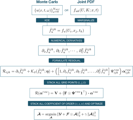
Following [8], our algorithm combines LASSO [31], i.e, $L_{1}$ regularization, with recursive feature elimination (RFE), which sequentially eliminates derivative features with small coefficients based on a tunable threshold at every iteration. This means that our algorithm has two hyper-parameters, $\gamma$ and the RFE threshold, which are chosen based on the test set error (rather than being part of the optimization variable $\mathbf{A}$) and a desired sparsity (i.e., a variance-bias balance). For this purpose, we test a few cross-validation algorithms for parameter estimation from Python’s scikit-learn package [17]. These algorithms, which rely on grid search to find the optimal regularization hyper-parameter $\gamma$, are LassoCV (an $n$-fold cross-validation set on each iteration), LassoLarsCV (an additional least-angle regression model), and LassoLarsIC (the Akaike or Bayes information criterion as an optimization variable over $\gamma$). They give very similar results when the optimal solution is in the vicinity of the hypothesis class, but might differ significantly when the solution is far from optimal. In general, the choice of the algorithm depends on whether one favors more sparsity or accuracy.

For $N_{\text{MC}}$ realizations of the random inputs, (1) is solved $N_{\text{MC}}$ times on the discretized space-time domain $D\times[0,T]$, yielding $N_{\text{MC}}$ solutions $u(\mathbf{x},t)$. These Monte Carlo results are then post-processed, e.g., with a Gaussian kernel density estimator (KDE) used in this study, to obtain the single-point PDF $f_{u}(U;\mathbf{x},t)$ on the discretized domain $D_{u}\times D\times[0,T]$. The KDE bandwidth is estimated for every grid point in $D\times[0,T]$ using Scott’s normal reference rule $h=3.49\,\sigma\,N_{\text{MC}}^{-1/3}$ [26], where $\sigma$ is the standard deviation of the data. The effect of the bandwidth on the solution is discussed in appendix D. Both the kernel type and the bandwidth are added hyper-parameters that can be optimized.

The matrices $\bm{\mathcal{V}}$ and $\bm{\mathcal{F}}$ in (13) can be very large, depending on the selected order of the polynomials ($R$, $S$ and $W$). We assume the coefficients to be time-independent, $\bm{\beta}=\bm{\beta}(U,\mathbf{x})$, so that $W=1$. This makes the resulting optimization problems numerically tractable on a personal computer. To increase the computational efficiency, we exclude grid points on which the labels, e.g., $\partial_{t}f_{u}(U;\mathbf{x},t)$, remain close to zero during the entire simulation. This sampling method leads to a significant reduction in computational cost (around a four-fold reduction in matrix size), especially in the case of a PDF that remains unchanged (equal zero) on the majority of the infinite domain.

To evaluate the generalization power of the method, we test its extrapolation power in time by fitting the hypothesis on the first $80\%$ of the time horizon $T$, i.e., on the domain $\mathcal{D}_{\text{train}}=D_{u}\times D\times[0,0.8T]$, and testing it on the remaining $20\%$ of the simulation, i.e., on $\mathcal{D}_{\text{test}}=D_{u}\times\mathcal{D}\times[0.8T,T]$).

3 Results

We validate our approach on a set of nonlinear problems with uncertain initial conditions and parameters. In these experiments, we use the method of distributions [29] to map the PDE (1) for the random field $u(\mathbf{x},t)$ onto either closed or unclosed PDEs of the marginal PDF $f_{u}(U;\mathbf{x},t)$. This illustrates the difficulties associated with analytical derivation of a PDF/CDF equation, and shows how our data-driven approach to PDE discover ameliorates them.

3.1 Nonlinear advection-reaction PDE with additive noise

This experiment, in which the derivation of a PDF equation is exact, serves to test the method’s accuracy in reconstruction of a PDF equation from $N_{\text{MC}}$ Monte Carlo runs. Let $u(x,t)$ be a real-valued state variable, whose dynamics is governed by

$$\frac{\partial u}{\partial t}+k\frac{\partial u}{\partial x}=rg(u),\qquad x\in\mathbb{R},\quad t\in\mathbb{R}^{+}$$ (14)

where $k\in\mathbb{R}^{+}$ and $r\in\mathbb{R}^{+}$ are deterministic advection and reaction rate constant, respectively. The initial condition $u(x,0)=u_{0}(x)$ is a random field with compact support in $\mathbb{R}$; it is characterized by a single-point PDF $f_{u_{0}}(U;x)$ and a two-point correlation function $\rho_{u_{0}}(x,y)$ specified for any two points $x,y\in\mathbb{R}$. The nonlinearity $g(u)$ is such that for any realization of $u_{0}(x)$ a solution of this problem, $u(x,t)$, is almost surely smooth. The PDF $f_{u}(U;x,t)$ satisfies exactly a PDE (A)

$$\frac{\partial f_{u}}{\partial t}+k\frac{\partial f_{u}}{\partial x}+r\frac{\partial g(U)f_{u}}{\partial U}=0,$$ (15)

subject to the initial condition $f_{u}(U;x,0)=f_{u_{0}}(U;x)$.

For the nonlinear source $g(u)=u^{2}$ used in this experiment, the analytical solution of (14) is $u(x,t)=[1/u_{0}(x-kt)-rt]^{-1}$. Uncertainty in the initial state, $u_{0}(x)=a\exp{[-(x-\mu)^{2}/(2\sigma^{2})]}$, is incapsulated in the real constants $a$, $\mu$, and $\sigma$. These parameters are sampled from independent Gaussian distributions, $a\sim\mathcal{N}(\eta_{a},\xi_{a})$, $\mu\sim\mathcal{N}(\eta_{\mu},\xi_{\mu})$, $\sigma\sim\mathcal{N}(\eta_{\sigma},\xi_{\sigma})$. The means and variances in these distributions are chosen to ensure that $u_{0}(x)$ almost surely has a compact support, $u(x\rightarrow\pm\infty,t)=0$, which ensures integrability of $u(x,\cdot)$ on $\mathbb{R}$. We set $k=1$, $r=1$, $T=0.5$, $\Delta t=0.0085$, $x\in[-2.0,3.0]$, $\Delta x=0.0218$, $\Delta U=0.0225$, $\eta_{a}=0.8$, $\xi_{a}=0.1$, $\eta_{\mu}=0.5$, $\xi_{\mu}=0.1$, $\eta_{\sigma}=0.45$, $\xi_{\sigma}=0.03$, and polynomial coefficients of order $M=3$ and $N=3$.

Figure 2: Error in estimation of the PDF $f_{u}$ on $\mathcal{D}_{\text{test}}$ (left) and the coefficients in the discovered PDF equation (16) (right) as function of the number of Monte Carlo realizations $N_{\text{MC}}$, without recursive feature elimination (RFE).

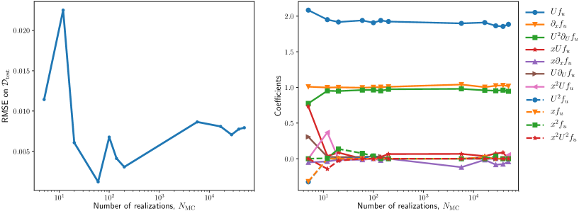
We use the grid search algorithm LassoCV to find $\gamma=0.0004$ that minimizes the test-set error, while seeking a sparse solution tunable by the RFE threshold. This direct equation learning (DEL) procedure leads to a PDE,

$$\frac{\partial\hat{f}_{u}}{\partial t}+\mathbf{0.996}\,\,\frac{\partial\hat{f}_{u}}{\partial x}+\mathbf{0.955}\,\,U^{2}\frac{\partial\hat{f}_{u}}{\partial U}+\mathbf{2.06}\,\,U\frac{\partial\hat{f}_{u}}{\partial U}=0,$$ (16)

which demonstrates our method’s ability to identify the relevant derivatives and their coefficients in equation (15) with $g(U)\equiv U^{2}$, eliminating all the remaining features in the dictionary $\mathcal{H}$; the original coefficients $k=1$ and $r=1$ are estimated with less than $5\%$ error. In the absence of recursive feature elimination, the algorithm yields 11 non-zero terms (Fig. 2), highlighting the importance of using RFE sparsification in addition to $L_{1}$ regularization. This is due to the variance-bias trade-off discussed in section 2.3.

The amount and quality of simulated data are characterized by two hyper-parameters: the number of Monte Carlo runs, $N_{\text{MC}}$, and the mesh size, $\Delta=\max\{\Delta U,\Delta x,\Delta t\}$. Figure 2 reveals that both the values of the coefficients $\bm{\beta}$ in the PDF equation (16) and the root mean square error (RMSE) its solution $\hat{f}_{u}$ in the extrapolation mode are relatively insensitive to $N_{\text{MC}}$ for around $N_{\text{MC}}>20$ realizations. This means that in this particular problem, the required number of Monte Carlo simulations is very small. But this is not always the case, as will be shown in section 3.3. The average RMSE is of order $\mathcal{O}(\Delta^{2})$, where $\Delta\approx 0.02$. This error is equivalent to a numerical scheme’s approximation error (a truncation error of the relevant Taylor expansion). The second-order error observed here is due to the use of a first-order finite difference scheme to create the derivative features. Higher-order accuracy can be obtained by using a more accurate numerical method, e.g., FFT, for calculating the derivatives.

Remark 2.

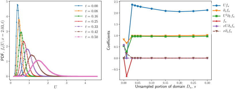
A solution $u(x,t)$ to (14) can be (nearly) deterministic in a part of the space-time domain $\mathcal{S}\in D\times[0,T]$, e.g., when $u(x,t)$ has a compact support; in this experiment the size of $\mathcal{S}$ is controlled by the support of the initial state $u_{0}(x)$ which is advected by (14) throughout the space-time domain $\mathbb{R}\times[0,T]$. This situation complicates the implementation of KDE and numerical differentiation, because the resulting PDF $f_{u}(U;x,t)$ is (close) to the Dirac delta function $\delta(\cdot)$; in this experiment, $f_{u}(U;x,t)\sim\delta(U)$ for $(x,t)\in\mathcal{S}$, as shown in Figure 3 for space-time points $(x=2.03,t)$ with small $t$. Consequently, a numerical implementation of our algorithm must provide an adequate approximation of the delta function and be able to handle sharp gradients with respect to $U$ in the neighborhood of $U=0$. (We found that rejecting data points near $u(x,t)=0$ from KDE leads to a poor MC approximation of $f_{u}(U;\cdot)$ and its derivatives, and to the discovery of an incorrect PDF equations on $\mathcal{D}_{\text{train}}$.) We address this issue by adding small perturbations $\xi$ to the initial state $u_{0}(x)$, i.e., by generating the training data from (14) subject to the initial condition $u^{\text{m}}_{0}(x)=\xi+u_{0}(x)$, where the random variable $\xi$ has the exponential PDF, $f_{\xi}(s)=\lambda\exp(-\lambda s)$ for $s\geq 0$ and $=0$ for $s<0$, with $\lambda\gg 1$ (in our experiments, $\lambda=10$). Another alternative is to omit training data from the simulation domain where the PDF has sharp profiles. In this case, the data in the domain $D^{o}_{u}\in[0,s|D_{u}|]$, with $s\in[0,1]$, are excluded from the training set $\mathcal{D}_{\text{train}}$ (Fig. 3b). Other strategies, which we defer for follow-up studies, include the discovery of PDF/CDF equations in the frequency domain.

Figure 3: PDF $f_{u}(U;x=2.03,t)$ (left) and the coefficient values in the discovered PDF equation using DEL (right) The effect of omitting training samples from the $U$ domain $D^{o}_{u}\in[0,s|D_{u}|]$, with $s\in[0,1]$, where the sharp PDF profiles complicate numerical differentiation. An RFE threshold of $0.1$ is used.

3.2 Nonlinear advection-reaction PDE with multiplicative noise

This test deals with a situation in which the exact PDF equation is not available and, hence, its multiple approximations have the right to exist, one of which we aim to discover. The setting is the same as in the previous section, except for the system parameter $k$ in (14) that is now random rather than deterministic. It is statistically independent from the random initial state $u_{0}(x)$ and has the PDF $f_{k}(K)$ with ensemble mean $\langle k\rangle$ and standard deviation $\sigma_{k}$. In the simulations reported below, we take $f_{k}(K)$ to be Gaussian with $\langle k\rangle=1$ and $\sigma_{k}=0.2$.

Figure 4: The coefficient values in the PDF equations, as function of the recursive feature elimination threshold, alternatively discovered via constrained equation learning (left), as in (7) or (17), and direct equation learning (right), as in (5).

The PDF $f_{u}(U;x,t)$ of the solution to this problem, $u(x,t)$, satisfies a PDE (A),

$$\frac{\partial f_{u}}{\partial t}+\langle k\rangle\frac{\partial f_{u}}{\partial x}+r\frac{\partial g(U)f_{u}}{\partial U}+\mathcal{C}(f_{u})=0.$$ (17)

This equation is formally exact but not computable since the operator $\mathcal{C}(f_{u})$ is unknown. It has to be conservative and is generally nonlocal [14, 15], taking the form of an integro-differential operator or, equivalently, a fractional-derivatives operator. One of its plausible approximations is (C)

$$\mathcal{C}(f_{u})=-\sigma_{k}^{2}\frac{\partial}{\partial x}\int_{0}^{t}\int_{D}\int_{D_{u}}G(U,V;x,y;t-\tau)\frac{\partial f_{u}}{\partial y}(V;y,\tau)\text{d}V\text{d}y\text{d}\tau,$$ (18)

where the kernel $G$ is the Green’s function of the two-dimensional advection equation. The spatiotemporal localization of (18) yields a PDF equation of the form (2). While one could include nonlocal terms in the dictionary $\mathcal{H}$, we leave this endeavor for future work; instead, our goal is to learn the localized version of $\mathcal{C}(f_{u})$ in (17). The resulting PDF equation, discovered via CEL (7), is compared with its counterpart discovered via DEL (5).

Figure 4 exhibits the coefficients of the PDF equations discovered with these two alternative strategies for equation discovery. These equations are not, and do not have to be, identical because the closure approximation is not unique. Nevertheless, the overall structure of the differential operators identified with the two strategies is largely consistent: the first eight most relevant features identified by direct learning, and two most relevant features in the learning with decomposition, involve the terms—$f_{u}$, $\partial_{x}f_{u}$ and $\partial_{U}f_{u}$—that must be present in the PDF equation based on the theoretical considerations leading to the unclosed PDE (17). The next most relevant term identified by both learning strategies is around $-0.02\partial_{x}^{2}f_{u}$, regardless of to the RFE threshold. Considering the value of $\sigma_{k}=0.2$, this is consistent with a theoretical diffusion-type localized closure $\mathcal{C}(f_{u})\approx-(\sigma_{k}^{2}/2)\partial_{x}^{2}f_{u}$ in (18).

Figure 4 reveals that the two learning strategies do differ in their identification of the variable coefficients $\bm{\beta}(U,x)$. For example, when small RFE thresholds are used, the direct learning identifies the coefficient of the feature $f_{u}$ to be $0.5+1.2U+0.35U^{2}$, instead of its counterpart $2U$ identified by the learning with decomposition. This discrepancy might either be a manifestation of non-uniqueness or reflect numerical differentiation error. Large RFE thresholds introduce additional dependency of this coefficient, $x^{2}U$.

Figure 5: Cross-validation error as function of the recursive feature elimination threshold for DEL (5) and CEL (17) (left). Cross-validation error as function of the extrapolation time fraction $\tau_{e}=t/T$ on the test set time domain $[0.7T,T]$, with corresponding training time domain $[0,0.7T]$ (right). The RMSE of the latter is lower because it is constrained by known derivative features, which reduces the hypothesis set.

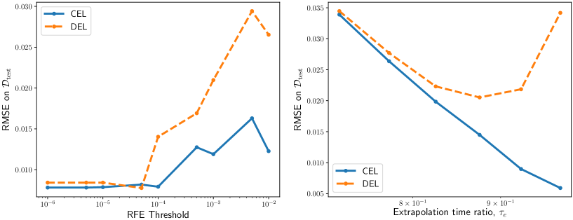
Over a wide range of the RFE threshold, learning with decomposition (17) outperforms direct learning (5) in terms of the RMSE on the test set (Fig. 5). This proves the point stated in section 2.3: constraining the hypothesis class with physics improves the approximation accuracy. That is, the more terms in a PDE we know, the more accurate the discovered PDE is likely to be.

Remark 3.

Given the lack of uniqueness, generalizability of a discovered PDE depends on the amount of information about the inputs one can transfer into its discovery. The PDF equation (17) with the closure $\mathcal{C}(f_{u})\approx-(\sigma_{k}^{2}/2)\partial_{x}^{2}f_{u}$ depends only on the first two moments of the random parameter $k$, its mean $\langle k\rangle$ and standard deviation $\sigma_{k}$, rather than on its full PDF $f_{k}(K)$. Hence, it might not generalize well to an arbitrary distribution of $k$. This can be remedied by learning a PDE for $f_{uk}(U,K;x,t)$, the joint PDF of the input $k$ and output $u(x,t)$. We show in B that the latter satisfies exactly an initial value problem

$$\frac{\partial f_{uk}}{\partial t}+K\frac{\partial f_{uk}}{\partial x}+r\frac{\partial g(U)f_{uk}}{\partial x}=0,\qquad f_{uk}(U,K;x,0)=f_{u_{0}}(U;x)f_{k}(K).$$ (19)

for any given input parameter distribution $f_{k}(K)$. This suggests that marginalization of $f_{uk}$ over $k$, i.e., transition from (19) to (17), transfers the information about $f_{k}(K)$ from the initial condition for the former to the differential operator in the latter; thus, leading to a weaker generalizability.

3.3 Nonlinear conservation laws

As a more nonlinear example of (1), we consider a smooth state variable $u(x,t)$ whose dynamics is governed by a hyperbolic conservation law with a nonlinear flux $g(u)$,

$$\frac{\partial u}{\partial t}+\frac{\partial g(u)}{\partial x}=0,\qquad u(x,0)=u_{0}(x),\qquad x\in\mathbb{R},\quad t>0.$$ (20)

Randomness comes from the uncertain initial state $u_{0}$, which is characterized by a single-point PDF $f_{u_{0}}(U;x)$ and a two-point correlation function $\rho_{u_{0}}(x,y)$. In the simulations reported below, we set $g(u)\equiv u^{2}/2$, i.e., analyze the inviscid Burgers equation; and $u_{0}(x)\equiv\xi+a\exp{[-(x-b)^{2}/(2c^{2})]}$ with Gaussian variables $\xi\sim\mathcal{N}(\eta_{\xi},\sigma_{\xi})$, $a\sim\mathcal{N}(\eta_{a},\sigma_{a})$, $b\sim\mathcal{N}(\eta_{b},\sigma_{b})$, and $c\sim\mathcal{N}(\eta_{c},\sigma_{c})$. We focus on the simulation time horizon $T$ before a shock develops. Once again, our goal is to discover a governing equation for $f_{u}(U;x,t)$, the single-point PDF of $u(x,t)$, from $N_{\text{MC}}$ Monte Carlo realizations of (20).

Figure 6: Error in estimation of the PDF $f_{u}$ on $\mathcal{D}_{\text{test}}$ (left) and the coefficients in the discovered PDF equation (right) for inviscid Burgers model without a shock. These are plotted as function of the number of Monte Carlo realizations $N_{\text{MC}}$, with the RFE threshold of $0.001$. Only the features whose values exceed $0.01$ are shown, out of $21$ non-zero features.

When applied to (20) with smooth solutions, the method of distributions yields the exact integro-differential equation [29]

$$\frac{\partial f_{u}}{\partial t}+g^{\prime}(U)\frac{\partial f_{u}}{\partial x}+g^{\prime\prime}(U)\frac{\partial F_{u}}{\partial x}=0,\qquad F_{u}(U;x,t)=\int_{-\infty}^{U}f_{u}(\tilde{U};x,t)\text{d}\tilde{U},$$ (21)

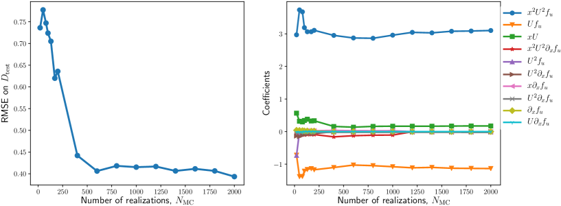
where $g^{\prime}(U)$ and $g^{\prime\prime}(U)$ are the first and second derivatives of $g(U)$, respectively. Its local approximation within the dictionary $\mathcal{H}$ in (4) is not unique. Given the superior behavior of CEL (7) observed above, we report in Figure 6 the results of this strategy only. The RMSE of predicted PDF $f_{u}$ over the test set $\mathcal{D}_{\text{test}}$ is an order of magnitude higher than in the previous experiments on advection-reaction equations. Both this error and the concomitant estimates of the coefficients in the learnt PDF equation require a larger number of Monte Carlo realizations to stabilize compared to the previous experiment, and that with a significant error.

An alternative to learning a PDF equation for $f_{u}(U;x,t)$ is to discover a CDF equation that governs the dynamics of $F_{u}(U;x,t)$, the single-point CDF of $u(x,t)$. The integration of (22) over $U$ leads to the PDE [29]

$$\frac{\partial F_{u}}{\partial t}+U\frac{\partial F_{u}}{\partial x}=0,$$ (22)

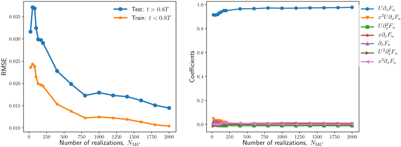
which is exact. Both the uniqueness of this CDF equation and the form of its differential operator suggest that its discovery from the dictionary $\mathcal{H}$ in (4) might be more tractable than the discovery of the corresponding PDF equation. Figure 7 demonstrates this to be case. In the absence of recursive feature elimination, the test set error is optimal when a few extra terms are included. These are advection ($\partial_{x}F_{u}$) and diffusion ($\partial_{x}^{2}F_{u}$) terms that account for Monte Carlo sampling error and its associated KDE approximation. When an RFE threshold of 0.03 is used, with $N_{\text{MC}}=50000$ realizations, the CDF equation is recovered almost exactly; with coefficient $1.001U$. This finding demonstrates the importance of choosing the “right” observable to learn. In this sense, it is akin to construction of reduced order models via the Koopman operator and dynamic mode decomposition [12, 13].

Figure 7: Error in estimation of the CDF $F_{u}$ on $\mathcal{D}_{\text{train}}$ and $\mathcal{D}_{\text{test}}$ (left) and the coefficients in the discovered CDF equation (right) for inviscid Burgers model without a shock. These are plotted as function of the number of Monte Carlo realizations $N_{\text{MC}}$. An RFE threshold of $0.001$ is used and only the features whose values exceed $0.01$ are shown, out of $22$ non-zero features.

The results presented above are for smooth solutions on the space-time domain before a shock or discontinuity develops. However, many nonlinear hyperbolic conservation laws (20), including the inviscid Burgers’ equation (20) with $g(u)\equiv u^{2}/2$, develop such discontinuities in finite time. When a shock develops, the PDE (20) is valid only in parts of the simulation domain where $u(x,t)$ is differentiable, and has to be supplemented with an equation for the position of and jump across the shock, i.e., with the Rankine-Hugoniot condition. Accordingly, PDF/CDF equations, such as (21) and (22), for problems with a shock are also invalid across the shock front and require special treatment [1, 34].

Specifically, (22) has to be replaced with [6]

$$\frac{\partial F_{u}}{\partial t}+U\frac{\partial F_{u}}{\partial x}=\beta_{1}(U,x,t),$$ (23)

This CDF equation is exact even in the presence of shocks; while the “kinetic defect” $\beta_{1}(U,x,t)$ is unique, its functional form is generally unknown. This equation falls within the dictionary $\mathcal{H}$ in (4) and, hence, has a chance of being discovered from $N_{\text{MC}}$ Monte Carlo realizations, $u^{(m)}(x,t)$ with $m=1,\ldots,N_{\text{MC}}$, of a solution to (20). These realizations are computed using a finite volume algorithm with a van Leer flux limiter to resolve the shock front without tracking its position. In this simulation, a periodic boundary condition is used.

As before, we explore two alternative strategies for equation discovery: DEL with the dictionary $\mathcal{H}$ in (4), and CEL in which only the source term $\beta_{1}(U,x,t)$ in (23) has to be learned. In both cases, the coefficients $\bm{\beta}$ are approximated with polynomials (8) in $U$ and $x$; their time dependence is reflected through the selection of training data. Let $t_{\text{sh}}^{(m)}$ with $m=1,\ldots,N_{\text{MC}}$ denote the shock breaking times in each of the $N_{\text{MC}}$ Monte Carlo realizations of (20). The test and training set sampling time interval $[t_{\text{st}},t_{\text{end}}]$ is chosen to contain the minimal shock breaking time $t_{\text{sh}}\equiv\min\{t_{\text{sh}}^{(1)},\ldots,t_{\text{sh}}^{(N_{\text{MC}})}\}$, such that $0\leq t_{\text{st}}\leq t_{\text{sh}}\leq t_{\text{end}}\leq T$. We investigate the relative importance of pre- and post-shock data in terms of the post-shock sampling fraction,

$$p_{s}=\frac{t_{\text{end}}-t_{\text{sh}}}{t_{\text{end}}-t_{\text{st}}}.$$ (24)

Figure 8 demonstrates the performance of the two learning strategies, DEL and CEL, as function of $p_{s}=t_{\text{end}}/t_{\text{sh}}-1$; the latter corresponds to the sampling time interval whose length is kept constant, $|t_{\text{end}}-t_{\text{st}}|=t_{\text{sh}}$, for all $p_{s}$. The results of the DEL approach (top row) show that the learning algorithm accounts for the shock by adding advection terms in both $U$ and $x$ but with an increasing RMS error as the sampling time domain enters the post-shock region $t>t_{\text{sh}}$. Compared to the DEL approach, CEL with only polynomial features (bottom row) starts with a smaller cross-validation error for $p_{s}<0.5$, showing the approximation power of this constrained approach, as justified by known existence theorems. The drastic increase in error for $p_{s}>0.5$ can be explained by the fact that i) the optimal source term $\beta_{1}(U,x,t)$ is typically time-dependent (here assumed time-independent) and ii) a polynomial approximation of $\beta_{1}$ cannot capture a spatially localized shock region.

Figure 8: Error in estimation of the CDF $F_{u}$ on $\mathcal{D}_{\text{test}}$ (left column) and the learned coefficients (right column) for the inviscid Burgers model with a shock. These are plotted as function of the post-shock sampling fraction, $p_{s}$, defined in (24). DEL identifies the differential operator for the CDF equation (top row), while CEL infers the polynomial representation of the kinetic defect term (bottom row). Only the features whose values exceed $0.01$ are shown, out of $23$ non-zero features in the top row, and $27$ features in the bottom row.

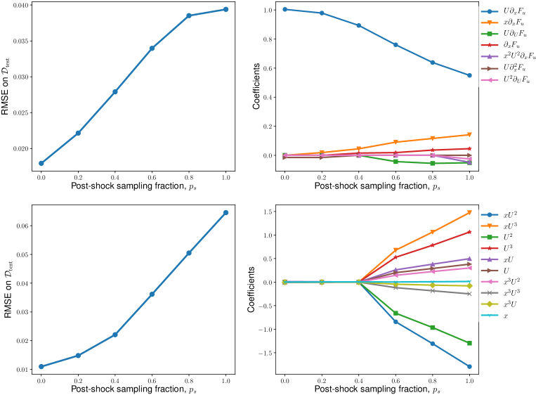
The similar trend in the change of the coefficients in CEL motivates the time-dependent representation of the kinetic defect $\beta_{1}(U,x,t)=\beta_{1}(U,x)\mathcal{I}(t\in[t_{\text{i}},t_{\text{i+1}}])$, where $\mathcal{I}$ is the indicator function for the membership in disjoint sampling intervals $[t_{\text{i}},t_{\text{i+1}}]$ on a regular grid, such that $i=0,\ldots,n-1$ and $n(t_{\text{i+1}}-t_{\text{i}})<T$. While this approach is computationally more expensive than including time polynomials in the source term, it does not assume a specific functional form. We will investigate this and other strategies for explicit treatment of time dependence in a follow-up study.

4 Discussion and conclusions

We presented a sparse-regression strategy for discovering coarse-grained equations from data generated with either a fine-scale model or Monte Carlo simulations of a model with random/uncertain coefficients and inputs. Motivated by the latter setting, we used this strategy to learn deterministic partial differential equations (PDEs) for the probability density function (PDF) or cumulative distribution function (CDF) of a random system state. The learning is not only data-driven but also physics-informed, in the sense that the construction of a dictionary of plausible terms in the differential operator, i.e., the formulation of scientific hypotheses, is driven by theoretical considerations such as the Pawula theorem [20, pp. 63-95]. Our sparse-regression strategy can be ran in two modes. The first, direct equation-learning (DEL), discovers a differential operator from the whole dictionary. The second, constrained equation learning (CEL), discovers only those terms in the differential operator that need to be discovered, i.e., learns closure approximations.

Our analysis leads to the following major conclusions.

• Discovery of PDF/CDF equations is advantageous because they are known to be linear and satisfy a number of theoretical constraints that reduce both the hypothesis set and the dictionary size.

• Selection of an observable whose dynamics is to be learned is key for successful equation discovery. In our example, the discovery of a CDF equation turned out to be significantly more robust than that of the corresponding PDF equation.

• The hyper-parameters used to fine-tune the algorithm, especially those used to generate and postprocess Monte Carlo data, play an important role in its performance. For example, the KDE bandwidth that leads to the accurate discovery of a differential operator can also add irrelevant terms.

• Our algorithm can be used to reverse-engineer black-box simulators by rediscovering the equations they solve from their output data. This can be used for solution verification, particularly when the solver does not strictly use rigorous numerical techniques, as occurs in physics-informed neural networks [18].

Future studies will deal with a number of theoretical and computational aspects of equation discovery, some of which are mentioned below. First, our framework provides a venue for hypothesis testing, since it relies on physical considerations to construct a dictionary of plausible terms in the operator. In this study, we constrained such a dictionary to the class of local models. Future studies will deal with account for nonlocality by incorporating integro-differential or fractional-derivative terms in the dictionary.

Second, the accuracy and computational efficiency of the proposed algorithm require further investigation and improvement. Future lines of research include the establishment of a relationship between a numerical scheme used to approximate the derivatives in a dictionary and the accuracy of learning; and the deployment of advanced techniques for optimization over tunable hyper-parameters such as the KDE bandwidth and the regularization coefficient.

Finally, we used a threshold on the labels $\partial_{t}f_{u}$ to exclude grid points on which the PDF does not change throughout the simulation from the training set. A more robust strategy might use the Kullback-Leibler divergence for feature elimination before running the optimization algorithm.

Appendix A Derivation of the PDF equation

Consider a generalized function

$$\pi_{u}(U-u)\equiv\delta(U-u(x,t)),$$ (25)

where $\delta(\cdot)$ is the Dirac delta function. If the random variable $u$ at any space-time point $(x,t)$ has a PDF $f_{u}(U;x,t)$, then, by definition of the ensemble average $\mathbb{E}[\cdot]$,

$$\begin{split}\mathbb{E}[\pi_{u}(U-u)]&=\int_{-\infty}^{+\infty}\pi_{u}(U-\tilde{U})f_{u}(\tilde{U};x,t)\text{d}\tilde{U}\\ &=\int_{-\infty}^{+\infty}\delta(U-\tilde{U})f_{u}(\tilde{U};x,t)\text{d}\tilde{U}\\ &=f_{u}(U;x,t).\end{split}$$ (26)

That is, the ensemble average of $\pi_{u}$ coincides with the single-point PDF of $u(x,t)$. This suggests a two-step procedure for derivation of PDF equations. First, one derives an equation for $\pi_{u}(U-u)$. Second, one ensemble-averages (homogenizes) the resulting equation.

The first step relies on rules of differential calculus applied, in the sense of distributions, to the function $\pi_{u}(U-u)$,

$$\frac{\partial\pi_{u}}{\partial u}=-\frac{\partial\pi_{u}}{\partial U},\qquad\frac{\partial\pi_{u}}{\partial t}=\frac{\partial\pi_{u}}{\partial u}\frac{\partial u}{\partial t}=-\frac{\partial\pi_{u}}{\partial U}\frac{\partial u}{\partial t},\qquad\frac{\partial\pi_{u}}{\partial x}=-\frac{\partial\pi_{u}}{\partial U}\frac{\partial u}{\partial x}.$$ (27)

Multiplying both sides of (14) with $\partial_{U}\pi_{u}$, using the above relations and the sifting property of the delta function, $g(u)\delta(U-u)=g(U)\delta(U-u)$ for any “good” function $g(u)$, we obtain a linear stochastic PDE for $\pi_{u}$,

$$\frac{\partial\pi_{u}}{\partial t}+k\frac{\partial\pi_{u}}{\partial x}+r\frac{\partial g(U)\pi_{u}}{\partial U}=0.$$ (28)

For deterministic parameters $k$ and $r$, the ensemble average of this PDE yields (15), a deterministic equation for the PDF $f_{u}(U;x,t)$. If one or two of these parameters are random (e.g., $k$), then ensemble averaging of this PDF is facilitated by a Reynolds decomposition that represents all the independent and dependent variables involved as the sums of their ensemble means and zero-mean fluctuations about these means, e.g., $k=\langle k\rangle+k^{\prime}$ and $\pi_{u}=f_{u}+\pi_{u}^{\prime}$ with $\mathbb{E}[k^{\prime}]=0$ and $\mathbb{E}[u^{\prime}(x,t)]=0$. For the deterministic $r$, the ensemble average of (28) yields an unclosed PDE for $f_{u}(U;x,t)$,

$$\frac{\partial f_{u}}{\partial t}+\langle k\rangle\frac{\partial f_{u}}{\partial x}+r\frac{\partial g(U)f_{u}}{\partial U}+\mathcal{C}(f_{u})=0,\qquad\mathcal{C}(f_{u})\equiv\mathbb{E}\left[k^{\prime}\frac{\partial\pi_{u}^{\prime}}{\partial x}\right]=\frac{\partial\mathbb{E}[k^{\prime}\pi_{u}^{\prime}]}{\partial x};$$ (29)

which is the same as (17).

Appendix B Derivation of the joint PDF equation

Consider a generalized function

$$\pi_{uk}(U-u,K-k)=\delta(U-u(x,t))\delta(K-k).$$ (30)

Let $f_{uk}(U,K;x,t)$ denote a joint PDF of the random input $k$ and the random output $u$ at any space-time point $(x,t)$. In analogy to (26), $\mathbb{E}[\pi_{uk}]=f_{uk}(U,K;x,t)$. A procedure similar to that used to derive a stochastic PDE (28) now yields a deterministic PDE for $\pi_{uk}$,

$$\frac{\partial\pi_{uk}}{\partial t}+K\frac{\partial\pi_{uk}}{\partial x}+\frac{\partial g(U)\pi_{uk}}{\partial U}=0.$$ (31)

The randomness of $\pi_{uk}$ stems from the random initial state $u_{0}$, rather than the model coefficients. Consequently, the averaging of this equation is trivial and exact, and given by (19). This equation is subject to the initial condition $f_{uk}(U,K;x,0)=f_{u_{0},k}(U,K;x)$. If $u_{0}(x)$ and $k$ are mutually independent, then $f_{uk}(U,K;x,0)=f_{u_{0}}(U;x)f_{k}(K)$.

The solution can be obtained numerically with a linear solver or, in some cases, analytically. For example, if $g(U)\equiv 0$, then the method of characteristics yields an exact PDF solution

$$f_{uk}(U,K;x,t)=f_{u_{0}}(U;x-Kt)f_{k}(K).$$ (32)

Appendix C Derivation of closure approximations

One way to approximate the mixed ensemble moment $C_{k\pi}=\langle k^{\prime}\pi_{u}^{\prime}\rangle$ in (29) is to subtract (29) from (28), giving an equation for the random fluctuations $\pi_{u}^{\prime}(U;x,t)$,

$$\frac{\partial\pi_{u}^{\prime}}{\partial t}+k^{\prime}\frac{\partial\pi_{u}^{\prime}}{\partial x}+k^{\prime}\frac{\partial f_{u}}{\partial x}+\langle k\rangle\frac{\partial\pi_{u}^{\prime}}{\partial x}+r\frac{\partial g(U)\pi_{u}^{\prime}}{\partial U}-\mathcal{C}(f_{u})=0.$$ (33)

Multiplying (33) by $k^{\prime}$ and taking the ensemble average, we obtain an unclosed PDE for $C_{k\pi}$,

$$\frac{\partial C_{k\pi}}{\partial t}+\frac{\partial\langle k^{\prime}k^{\prime}\pi_{u}^{\prime}\rangle}{\partial x}+\langle k^{\prime}k^{\prime}\rangle\frac{\partial f_{u}}{\partial x}+\langle k\rangle\frac{\partial C_{k\pi}}{\partial x}-\frac{\partial\langle k^{\prime}k^{\prime}\pi_{u}^{\prime}\rangle}{\partial x}+\frac{\partial g(U)C_{k\pi}}{\partial U}=0.$$ (34)

This equation is closed by neglecting the third-order term, $\langle k^{\prime}k^{\prime}\pi_{u}^{\prime}\rangle$, which yields a two-dimensional advection equation for $C_{k\pi}$,

$$\frac{\partial C_{k\pi}}{\partial t}+\langle k\rangle\frac{\partial C_{k\pi}}{\partial x}+\frac{\partial g(U)C_{k\pi}}{\partial U}=-\sigma_{k}^{2}\frac{\partial f_{u}}{\partial x}.$$ (35)

A closed system of PDEs (29) and (35) defines the joint dynamics of two dependent variables, $f_{u}(U;x,t)$ and $C_{k\pi}(U;x,t)$. To reduce this system to a single equation for $f_{u}(U;x,t)$, we write the solution of (35) as

$$C_{k\pi}(U;x,t)=-\sigma_{k}^{2}\int_{0}^{t}\int_{-\infty}^{+\infty}\int_{D_{u}}G(U,V;x,y;t-\tau)\frac{\partial f_{u}(V;y,\tau)}{\partial y}\text{d}V\text{d}y\text{d}\tau,$$ (36)

where $G(U,V;x,y;t-\tau)$ is the Green’s function for (35), defined as the solution of $\partial_{t}G-\mathbf{U}\cdot\nabla_{\tilde{\mathbf{x}}}G=\delta(U-V)\delta(x-y)\delta(t-\tau)$ subject to the homogeneous initial and boundary conditions. Here, $\tilde{\mathbf{x}}=(x,U)^{\top}$ and $\mathbf{U}=(\langle k\rangle,g(U))^{\top}$. Taking the derivative of this solution with respect to $x$ leads directly to (18).

Appendix D Hyper-parameter tuning

Hyper-parameter tuning can significantly increase the optimization dimensionality. To avoid this, we investigate the dependence of RMSE on two of these parameters: the polynomial order used to represent the coefficients $\bm{\beta}$ and the KDE bandwidth used to process Monte Carlo realizations. The polynomial order increases the representation accuracy but decreases the sparsity of the discovered PDEs. Figure 9 reveals that the sparsity reaches a plateau at polynomial order of $2$. This is the order we use in the numerical experiments reported in section 3.

Figure 9: RMSE and sparsity in the closure as function of the polynomial order in the advection-reaction closure problem of section 3.2. The results show marginal gains in accuracy and sparsity when the polynomial order is $\geq 2$.

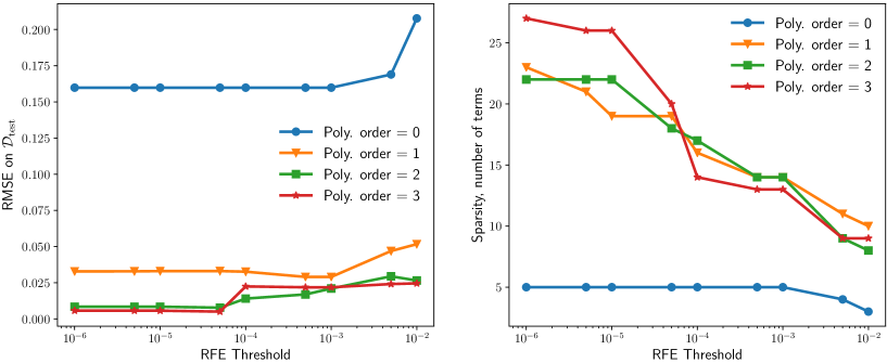
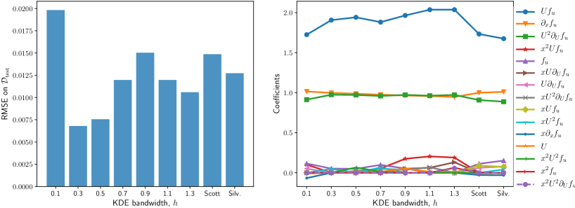
Figure 10 demonstrates that the KDE bandwidth plays a big role in the accuracy of an estimated PDF $f_{u}$ and its corresponding derivatives. We found that Scott’s or Silverman’s rule for estimating the bandwidth does not guarantee optimal coefficients, in comparison to fixed bandwidths. On the other hand, a bandwidth of $h=1.3$ leads to accurate estimates of the relevant model coefficients, but also adds irrelevant terms with large coefficients.

Figure 10: Error and coefficients as function of the KDE bandwidth.

References

- Alawadhi et al. [2018] A. Alawadhi, F. Boso, and D. M. Tartakovsky. Method of distributions for water-hammer equations with uncertain parameters. Water Resour. Res., 54(11):9398–9411, 2018.
- Barajas-Solano and Tartakovsky [2016] D. Barajas-Solano and A. M. Tartakovsky. Probabilistic density function method for nonlinear dynamical systems driven by colored noise. Phys. Rev. E, 93:052121, 2016.
- Boso and Tartakovsky [2016] F. Boso and D. M. Tartakovsky. The method of distributions for dispersive transport in porous media with uncertain hydraulic properties. Water Resour. Res., 52(6):4700–4712, 2016. doi: 10.1002/2016WR018745.
- Boso and Tartakovsky [2018] F. Boso and D. M. Tartakovsky. Information-theoretic approach to bidirectional scaling. Water Resour. Res., 54(7):4916–4928, 2018.
- Boso and Tartakovsky [2020a] F. Boso and D. M. Tartakovsky. Learning on dynamic statistical manifolds. Proc. Roy. Soc. A, page 20200213, 2020a. doi: 10.1098/rspa.2020-0213.
- Boso and Tartakovsky [2020b] F. Boso and D. M. Tartakovsky. Data-informed method of distributions for hyperbolic conservation laws. SIAM J. Sci. Comput., 42(1):A559–A583, 2020b. doi: 10.1137/19M1260773.
- Boso et al. [2014] F. Boso, S. V. Broyda, and D. M. Tartakovsky. Cumulative distribution function solutions of advection-reaction equations with uncertain parameters. Proc. R. Soc. A, 470(2166):20140189, 2014. doi: 10.1098/rspa.2014.0189.
- Brunton et al. [2016] S. L. Brunton, J. L. Proctor, J. N. Kutz, and W. Bialek. Discovering governing equations from data by sparse identification of nonlinear dynamical systems. Proc. Natl. Acad. Sci. U.S.A., 113(15):3932–3937, 2016.
- Felsberger and Koutsourelakis [2018] L. Felsberger and P. Koutsourelakis. Physics-constrained, data-driven discovery of coarse-grained dynamics. Comm. Comput. Phys., 25, 2018. doi: 10.4208/cicp.OA-2018-0174.
- Geneva and Zabaras [2019] N. Geneva and N. Zabaras. Quantifying model form uncertainty in Reynolds-averaged turbulence models with Bayesian deep neural networks. J. Comput. Phys., 383:125–147, 2019.
- Geneva and Zabaras [2020] N. Geneva and N. Zabaras. Modeling the dynamics of PDE systems with physics-constrained deep auto-regressive networks. J. Comput. Phys., 403:109056, 2020. doi: 10.1016/j.jcp.2019.109056.
- Lu and Tartakovsky [2020a] H. Lu and D. M. Tartakovsky. Lagrangian dynamic mode decomposition for construction of reduced-order models of advection-dominated phenomena. J. Comput. Phys., 407:109229, 2020a. doi: 10.1016/j.jcp.2020.109229.
- Lu and Tartakovsky [2020b] H. Lu and D. M. Tartakovsky. Prediction accuracy of dynamic mode decomposition. SIAM J. Sci. Comput., 42(3):A1639–A1662, 2020b. doi: 10.1137/19M1259948.
- Maltba et al. [2018] T. Maltba, P. Gremaud, and D. M. Tartakovsky. Nonlocal PDF methods for Langevin equations with colored noise. J. Comput. Phys., 367:87–101, 2018.
- Neuman and Tartakovsky [2009] S. P. Neuman and D. M. Tartakovsky. Perspective on theories of anomalous transport in heterogeneous media. Adv. Water Resour., 32(5):670–680, 2009. doi: 10.1016/j.advwatres.2008.08.005.
- Pang et al. [2019] G. Pang, L. Lu, and G. E. Karniadakis. fpinns: Fractional physics-informed neural networks. SIAM J. Sci. Comput., 41(4):A2603–A2626, 2019.
- Pedregosa et al. [2011] F. Pedregosa, G. Varoquaux, A. Gramfort, V. Michel, B. Thirion, O. Grisel, M. Blondel, P. Prettenhofer, R. Weiss, V. Dubourg, J. Vanderplas, A. Passos, D. Cournapeau, M. Brucher, M. Perrot, and E. Duchesnay. Scikit-learn: Machine learning in Python. J. Mach. Learn. Res., 12:2825–2830, 2011.
- Raissi et al. [2017] M. Raissi, P. Perdikaris, and G. E. Karniadakis. Machine learning of linear differential equations using Gaussian processes. J. Comput. Phys., 348:683–693, 2017.
- Raissi et al. [2019] M. Raissi, P. Perdikaris, and G. E. Karniadakis. Physics-informed neural networks: A deep learning framework for solving forward and inverse problems involving nonlinear partial differential equations. J. Comput. Phys., 378:686–707, 2019.
- Risken [1989] H. Risken. The Fokker-Planck Equation: Methods of Solution and Applications. Springer-Verlag, New York, 2nd edition, 1989.
- Rudy et al. [2019] S. Rudy, A. Alla, S. L. Brunton, and J. N. Kutz. Data-driven identification of parametric partial differential equations. SIAM J. Appl. Dyn. Syst., 18(2):643–660, 2019.
- Rudy et al. [2017] S. H. Rudy, S. L. Brunton, J. L. Proctor, and J. N. Kutz. Data-driven discovery of partial differential equations. Sci. Adv., 3(4):1–7, 2017.
- Schaeffer [2017] H. Schaeffer. Learning partial differential equations via data discovery and sparse optimization. Proc. Roy. Soc. A, 473(2197), 2017. doi: 10.1098/rspa.2016.0446.
- Schmidt and Lipson [2009] M. Schmidt and H. Lipson. Distilling free-form natural laws from experimental data. Science, 324(5923):81–85, 2009.
- Schöberl et al. [2017] M. Schöberl, N. Zabaras, and P.-S. Koutsourelakis. Predictive coarse-graining. J. Comput. Phys., 333:49–77, 2017.
- Scott [1979] D. W. Scott. On optimal and data-based histograms. Biometrika, 66(3):605–610, 1979.
- Sirignano and Spiliopoulos [2018] J. Sirignano and K. Spiliopoulos. DGM: A deep learning algorithm for solving partial differential equations. J. Comput. Phys., 375:1339–1364, 2018.
- Tartakovsky et al. [2020] A. M. Tartakovsky, C. Ortiz Marrero, P. Perdikaris, G. D. Tartakovsky, and D. Barajas‐Solano. Physics‐informed deep neural networks for learning parameters and constitutive relationships in subsurface flow problems. Water Resour. Res., 56(5):e2019WR026731, 2020.
- Tartakovsky and Gremaud [2016] D. M. Tartakovsky and P. A. Gremaud. Method of distributions for uncertainty quantification. In R. Ghanem, D. Higdon, and H. Owhadi, editors, Handbook of Uncertainty Quantification. Springer International Publishing, Switzerland, 2016. doi: 10.1007/978-3-319-11259-6.27-1.
- Taverniers and Tartakovsky [2020] S. Taverniers and D. M. Tartakovsky. Estimation of distributions via multilevel monte carlo with stratified sampling. J. Comput. Phys., 419:109572, 2020. doi: 10.1016/j.jcp.2020.109572.
- Tibshirani [1996] R. Tibshirani. Regression shrinkage and selection via the lasso. J. Roy. Stat. Soc. B, 58(1):267–288, 1996.
- Venturi et al. [2013] D. Venturi, D. M. Tartakovsky, A. M. Tartakovsky, and G. E. Karniadakis. Exact PDF equations and closure approximations for advective-reactive transport. J. Comput. Phys., 243:323–343, 2013.
- Wang et al. [2013a] P. Wang, A. M. Tartakovsky, and D. M. Tartakovsky. Probability density function method for Langevin equations with colored noise. Phys. Rev. Lett., 110(14):140602, 2013a. doi: 10.1103/PhysRevLett.110.140602.
- Wang et al. [2013b] P. Wang, D. M. Tartakovsky, J. K. D. Jarman, and A. M. Tartakovsky. CDF solutions of Buckley–Leverett equation with uncertain parameters. Multiscale Model. Simul., 11(1):118–133, 2013b. doi: 10.1137/120865574.
- Winter et al. [2003] C. L. Winter, D. M. Tartakovsky, and A. Guadagnini. Moment equations for flow in highly heterogeneous porous media. Surv. Geophys., 24(1):81–106, 2003.
- Wu and Xiu [2020] K. Wu and D. Xiu. Data-driven deep learning of partial differential equations in modal space. J. Comput. Phys., 408:109307, 2020. doi: 10.1016/j.jcp.2020.109307.
- Yang et al. [2019] H.-J. Yang, F. Boso, H. A. Tchelepi, and D. M. Tartakovsky. Probabilistic forecast of single-phase flow in porous media with uncertain properties. Water Resour. Res., 55(11):8631–8645, 2019.