Overcoming Output Constraints in Iterative Learning Control Systems by Reference Adaptation

Abstract

Iterative Learning Control (ILC) schemes can guarantee properties such as asymptotic stability and monotonic error convergence, but do not, in general, ensure adherence to output constraints. The topic of this paper is the design of a reference-adapting ILC (RAILC) scheme, extending an existing ILC system and capable of complying with output constraints. The underlying idea is to scale the reference at every trial by using a conservative estimate of the output’s progression. Properties as the monotonic convergence above a threshold and the respect of output constraints are formally proven. Numerical simulations and experimental results reinforce our theoretical results.

1 Introduction

Iterative Learning Control (ILC) is a control scheme suitable for systems operating in a repetitive manner. ILC tracks a desired reference and aims at improving its accuracy from repetition to repetition by exploiting the information of previous trials, see Bristow et al. (2006) for a survey. ILC can achieve better performance than conventional feedback systems as the latter does not exploit available information from previous trials, see, e.g., Moore et al. (1992). ILC finds much appeal in fields such as robotics, manufacturing, and biomedical applications due to the possibility of repeating trials; such fields have greatly benefited from the implementation of ILC systems, see, e.g. Elci et al. (2002), Seel et al. (2011), Rogers and Tutty (2016), and Pandit and Buchheit (1999).

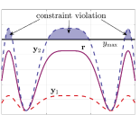
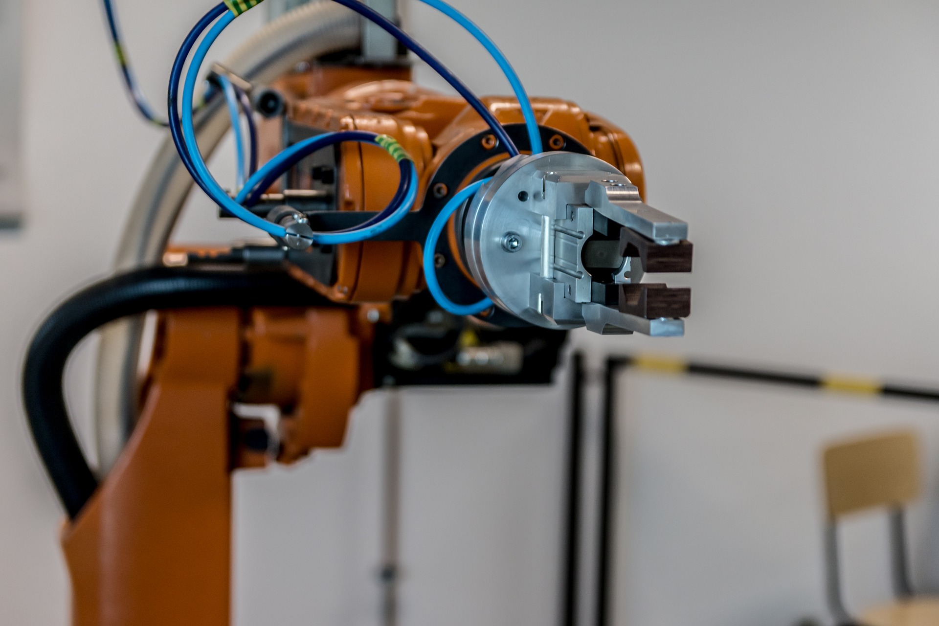
A relevant class of systems for ILC applications are those subject to output constraints. A robotic manipulator, for example, is commonly restricted when it comes to possible positions and paths; violating these constraints may potentially damage the system. In general, ILC systems can guarantee monotonic error convergence, meaning that the difference between the output and the desired trajectory decreases in a suitable norm at every trial. However, compliance with output constraints is, in general, not guaranteed. For example, Fig. 1 depicts an ILC system learning the desired trajectory $\mathbf{r}$ while being constrained by the maximum value $y_{\mathrm{max}}$.

Figure 1: Illustration of the output-constrained ILC problem and a robotic manipulator restricted by output constraints

Although the system is monotonically convergent, the output constraints are violated during the second trial. This paper addresses this problem and proposes a modular solution extending the ILC system, thus ensuring compliance with the output constraints while maintaining monotonic error convergence.

Output-constrained ILC systems have already been investigated elsewhere and can be classified in two different categories. In the first class, novel update laws based on constrained optimization have been introduced. For example, Jin et al. (2014) propose an update-law based on a high-dimensional and constrained optimization problem. This requires accurate knowledge of the plant dynamics to ensure compliance with the output constraints in time-varying ILC systems. In the second class, methods like the one proposed by Sebastian et al. (2018a) combine ILC with additional feedback control to handle linear, time-varying, multi-input multi-output systems with input and output constraints. Sebastian et al. (2018b) validate this approach for a robotic manipulator where an underlying feedback controller is implemented to avoid the violation of constraints.

The approach in this paper is to update the reference trajectory for each trial based on a low-dimensional optimization problem. It does not require accurate knowledge of the plant dynamics and ensures compliance with the output constraints while maintaining the existing ILC system’s monotonic error convergence. In contrast to previous work, the proposed RAILC scheme is a modular extension requiring neither high-dimensional optimization nor the design of an underlying feedback controller. The proposed method is validated using a two-wheeled inverted pendulum robot (TWIPR), whose task is to learn a highly accurate motion in the presence of output constraints.

The remainder of this paper is structured as follows. Section 2 introduces notation. Section 3 briefly summarizes the structure of conventional ILC system consisting of a linear plant, learning function, and Q-filter. Section 4 formulates the problem. Section 5 introduces a RAILC algorithm and discusses its properties formally. Section 6 presents a TWIPR and validates the RAILC scheme in both simulation and experiment. The simulation results of the RAILC algorithm are also compared to those of the conventional ILC. Finally, Section 7 gives concluding remarks.

2 Notation

Let $\rm I\!N_{\mathrm{0}}$ and $\rm I\!N$ denote the set of nonnegative, respectively positive, integers, $\rm I\!R$ the set of real numbers and $\rm I\!R_{>0}$, respectively $\rm I\!R_{\geq 0}$, the set of positive, respectively nonnegative, real numbers. Vectors are in bold type and lower-case letters, e.g., $\mathbf{v}$. Matrices are in bold type and upper-case letters, e.g., $\mathbf{A}$. Matrix $\mathbf{A}^{T}$ denotes the transpose of the matrix $\mathbf{A}$. Indices of vectors are used to denote the ILC trial, e.g., $\mathbf{v}_{j}$ denotes the vector $\mathbf{v}$ on the $j^{\mathrm{th}}$ ILC trial. Let $\left|\left|{\mathbf{v}}\right|\right|$ denote a norm of the vector $\mathbf{v}$, and $\left|\left|{\mathbf{A}}\right|\right|$ the corresponding, induced matrix norm of the matrix $\mathbf{\mathbf{A}}$. Particular examples are the Euclidean norm, denoted by $\left|\left|{\boldsymbol{\cdot}}\right|\right|_{2}$, and the infinite norm, denoted by $\left|\left|{\boldsymbol{\cdot}}\right|\right|_{\infty}$. The spectral radius of a square matrix $\mathbf{A}$ is denoted by $\rho\left(\mathbf{A}\right)$. The maximum singular value of matrix $\mathbf{A}$ is denoted by $\overline{\sigma}\left(\mathbf{A}\right)$.

3 Lifted-System ILC in a Nutshell

Consider the discrete-time, linear, time-invariant SISO system at its $j^{\mathrm{th}}$ trial, $j\in\rm I\!N_{\mathrm{0}}$,

$$\left\{\begin{array}[]{cl}\mathbf{x}_{j}(n+1)&=\mathbf{A}\mathbf{x}_{j}(n)+\mathbf{B}u_{j}(n)+d(n)\\ y_{j}(n)&=\mathbf{C}\mathbf{x}_{j}(n)\end{array}\right.\,,$$ (1)

where $n\in\left\{1,...,N\right\}$ is the sample index and $N\in\rm I\!N$ is the numbers of samples in each trial. Let, $\forall n\in\left\{1,...,N\right\}$, $\mathbf{x}(n)\in\rm I\!R^{k}$ denote the $k$ dimensional state vector, $u(n)\in\rm I\!R$ the input variable, $y(n)\in\rm I\!R$ the output variable and $d(n)\in\rm I\!R$ an unknown disturbance, which is the same for all trials. Let $\mathbf{A}\in\rm I\!R^{k\times k}$ denote the system matrix, $\mathbf{B}\in\rm I\!R^{k\times 1}$ the input matrix, and $\mathbf{C}\in\rm I\!R^{1\times k}$ the output matrix.

System (1) can be rewritten in its so-called lifted form, i.e.,

$$\mathbf{y}_{j}=\mathbf{P}\mathbf{u}_{j}+\mathbf{d}\,,$$ (2)

where, at each iteration $j\in\rm I\!N_{\mathrm{0}}$,

$$\mathbf{u}_{j} =\begin{bmatrix}u_{j}(0)&u_{j}(1)&\dots&u_{j}(N-1)\end{bmatrix}^{T}$$ (3a)

$$\mathbf{y}_{j} =\begin{bmatrix}y_{j}(m)&y_{j}(m+1)&\dots&y_{j}(m+N-1)\end{bmatrix}^{T}$$ (3b)

$$\mathbf{d} =\begin{bmatrix}d(m)&d(m+1)&\dots&d(m+N-1)\end{bmatrix}^{T}$$ (3c)

and $m\in\rm I\!N_{\mathrm{0}}$ denotes the system’s relative degree, see Bristow et al. (2006). For system (1) the parameters $p_{ij}\in\rm I\!R$ of the plant matrix $\mathbf{P}$ are given by

$$\forall i,j\in\rm I\!N\qquad p_{ij}=\left\{\begin{array}[]{cl}\mathbf{C}\mathbf{A}^{i-j+m-1}\mathbf{B}&\forall i\geq j\\ 0&\forall i<j\end{array}\right.\,.$$ (4)

The goal of an ILC system is to have output $\mathbf{y}_{j}$ follow a desired trajectory $\mathbf{r}\in\rm I\!R^{N}$. To this end, a learning matrix, namely $\mathbf{L}\in\rm I\!R^{N\times N}$, and a Q-filter, namely $\mathbf{Q}\in\rm I\!R^{N\times N}$, need to be designed (see, e.g. Bristow et al. (2006)), thus leading to the update law

$$\forall j\in\rm I\!N,\qquad\mathbf{u}_{j+1}=\mathbf{Q}\left(\mathbf{u}_{j}+\mathbf{L}\mathbf{e}_{j}\right)\,,$$ (5)

where $\mathbf{e}_{j}\in\rm I\!R^{N}$ denotes the error trajectory defined as

$$\forall j\in\rm I\!N,\qquad\mathbf{e}_{j}:=\mathbf{r}-\mathbf{y}_{j}\,.$$ (6)

Note that the matrices $\mathbf{P}$, $\mathbf{L}$ and $\mathbf{Q}$ are regular.

Definition 1

(Asymptotic Stability, see Bristow et al. (2006)): The ILC system with dynamics (2) and update law (5) is asymptotically stable if the limit

$$\mathbf{e}_{\infty}: =\lim_{j\rightarrow\infty}\mathbf{e}_{j}$$

$$=\left[\mathbf{I}-\mathbf{P}\left[\mathbf{I}-\mathbf{Q}\left(\mathbf{I}-\mathbf{L}\mathbf{P}\right)\right]^{-1}\mathbf{Q}\mathbf{L}\right]\left(\mathbf{r}-\mathbf{d}\right)$$ (7)

uniquely exists. In what follows, let $\mathbf{e}_{\infty}$ be named residual error.

Note that, if $\mathbf{Q}=\mathbf{I}$, by (7), $\mathbf{e}_{\infty}=0$.

Proposition 1

(Bristow et al., 2006, Theorem 1)s The ILC system with dynamics (2) and update law (5) is asymptotically stable if and only if

$$\rho\left(\mathbf{Q}\left(\mathbf{I}-\mathbf{L}\mathbf{P}\right)\right)<1\,.$$ (8)

See (Bristow et al., 2006, Theorem 1).

Despite asymptotic stability, the error trajectory can take arbitrarily large values, thus generating large learning transients. The concept of monotonic convergence narrows the set of possible error trajectories.

Definition 2

(Monotonic Convergence, see Bristow et al. (2006)): The system composed of plant (2) and update law (5) is monotonically convergent under a given norm $\left|\left|{\boldsymbol{\cdot}}\right|\right|$ if

$$\forall j\in\rm I\!N_{\mathrm{0}},\quad\left|\left|{\mathbf{e}_{\infty}-\mathbf{e}_{j+1}}\right|\right|\leq\gamma\left|\left|{\mathbf{e}_{\infty}-\mathbf{e}_{j}}\right|\right|\,,$$ (9)

where $\gamma\in[0,1)$ is the convergence rate.

Proposition 2

The system (2)-(5) is monotonically convergent under a given norm $\left|\left|{\boldsymbol{\cdot}}\right|\right|$ if

$$\gamma:=\left|\left|{\mathbf{P}\mathbf{Q}\left(\mathbf{I}-\mathbf{L}\mathbf{P}\right)\mathbf{P}^{-1}}\right|\right|<1\,.$$ (10)

See Bristow et al. (2006).

Monotonic convergence is traditionally verified for the spectral and the infinite norms, i.e., respectively,

$$\gamma_{\mathrm{2}} :=\overline{\sigma}\left(\mathbf{P}\mathbf{Q}\left(\mathbf{I}-\mathbf{L}\mathbf{P}\right)\mathbf{P}^{-1}\right)$$ (11)

and

$$\gamma_{\infty} :=\left|\left|{\mathbf{P}\mathbf{Q}\left(\mathbf{I}-\mathbf{L}\mathbf{P}\right)\mathbf{P}^{-1}}\right|\right|_{\infty}\,.$$ (12)

Definition 3

(Monotonic convergence above athreshold, see Seel et al. (2017)): System (2)-(5) is monotonically convergent above a threshold $\kappa\in\rm I\!R_{\geq 0}$ under a given norm $\left|\left|{\boldsymbol{\cdot}}\right|\right|$ if

$$\forall j\in\rm I\!N_{\mathrm{0}}:\left|\left|{\mathbf{e}_{j}}\right|\right|\geq\kappa\quad\implies\left|\left|{\mathbf{e}_{j+1}}\right|\right|\leq\left|\left|{\mathbf{e}_{j}}\right|\right|\,.$$ (13)

Proposition 3

(Seel et al., 2017, Theorem 1) System (2)-(5) is monotonically convergent above the threshold $\epsilon=\left|\left|{\left(\mathbf{I}-\mathbf{P}\mathbf{Q}\mathbf{P}^{-1}\right)\left(\mathbf{r}-\mathbf{d}\right)}\right|\right|$ under a given norm $\left|\left|{\boldsymbol{\cdot}}\right|\right|$ if

$$\gamma<1\,.$$ (14)

See (Seel et al., 2017, Theorem 1).

By Propositions 1-3, to ensure properties as asymptotic stability and monotonic convergence, standard design methods, see, e.g., Bristow et al. (2006), can be employed. Commonly, the Q-filter is chosen as a low-pass filter so that frequencies above its bandwidth are cut-off from the learning, thus increasing robustness. The learning matrix $\mathbf{L}$ is typically designed by either tuning the parameters of a PD-function, applying $\mathcal{H}_{\infty}$ optimization, or by solving a quadratic optimal problem.

4 Problem Formulation

Consider system (2)-(5) with a desired trajectory $\mathbf{r}$. Both the Q-filter and the learning matrix are designed such that asymptotic stability and monotonic error convergence are guaranteed.

Additionally, the output $\mathbf{y}_{j}$ is constrained by an upper bound $y_{\mathrm{max}}\in\rm I\!R_{>0}$, which must not be violated on any trial, i.e.,

$$\forall j\in\rm I\!N_{\mathrm{0}},\qquad\left|\left|{\mathbf{y}_{j}}\right|\right|_{\infty}<y_{\mathrm{max}}\,.$$ (15)

Despite monotonic convergence, the conventional ILC system does not necessarily enforce output constraints (see Fig. 1). We propose to extend the designed ILC in a modular fashion, so that output constraints are satisfied and monotonic error convergence maintained.

To ensure the problem being well-posed, some assumptions are needed.

Assumption 1

There is a known initial input trajectory $\mathbf{u}_{\mathrm{0}}$ leading to an initial output trajectory $\mathbf{y}_{\mathrm{0}}$ such that

$$\left|\left|{\mathbf{y}_{\mathrm{0}}}\right|\right|_{\infty}\leq y_{\mathrm{max}}\,.$$ (16)

Assumption 2

The reference trajectory $\mathbf{r}$ is chosen such that

$$\left|\left|{\mathbf{r}}\right|\right|_{\infty}\leq y_{\mathrm{max}}\,.$$ (17)

5 Reference-Adapting ILC

The basic idea of this reference-adapting iterative learning control (RAILC) scheme is to adapt the reference trajectory $\mathbf{r}$ at each ILC trial to ensure that the output trajectory $\mathbf{y}_{j}$ does not exceed the maximum value $y_{\mathrm{max}}$. To this end, let

$$\forall j\in\rm I\!N_{\mathrm{0}},\qquad{\mathbf{r}}_{j}\in\rm I\!R^{N}$$ (18)

denote the adapted reference trajectory at the $j^{\mathrm{th}}$ trial leading to the adapted update law

$$\forall j\in\rm I\!N_{\mathrm{0}},\qquad\mathbf{u}_{j+1}=\mathbf{Q}\left(\mathbf{u}_{j}+\mathbf{L}\left({\mathbf{r}}_{j}-\mathbf{y}_{j}\right)\right)\,.$$ (19)

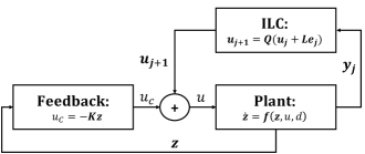
Figure 2: Block diagram of the RAILC system

Let $\overline{\epsilon}\in\rm I\!R$ denote an upper bound such that

$$\overline{\epsilon}\geq\max_{\forall j\in\rm I\!N}{\left|\left|{\left(\mathbf{I}-\mathbf{P}\mathbf{Q}\mathbf{P}^{-1}\right)\left({\mathbf{r}}_{j}-\mathbf{d}\right)}\right|\right|_{\infty}}\,.$$ (20)

Algorithm 1

The adapted reference trajectory ${\mathbf{r}}_{j}$ is

$$\forall j\in\rm I\!N_{\mathrm{0}},\qquad{\mathbf{r}}_{j}:=\mathbf{y}_{j}+a_{j}\left(\mathbf{r}-\mathbf{y}_{j}\right)$$ (21)

with

$$a_{j}=\max\tilde{a}_{j}$$ (22a)

$$\mathrm{s.t.}\quad \tilde{a}_{j}\in[0,1]$$ (22b)

$$\tilde{a}_{j}\leq\frac{y_{\mathrm{max}}-\left|\left|{\mathbf{y}_{j}+\tilde{a}_{j}(\mathbf{r}-\mathbf{y}_{j})}\right|\right|_{\infty}-\overline{\epsilon}}{\gamma_{\infty}\left|\left|{\mathbf{r}-\mathbf{y}_{j}}\right|\right|_{\infty}}$$ (22c)

Note that the optimization problem (22) can be efficiently solved using bisection, which makes the algorithm applicable to embedded systems with low computational power.

Consider the upper bound $\overline{\epsilon}$ required to solve the optimization problem (22). In the trivial case of $\mathbf{Q}=\mathbf{I}$, $\overline{\epsilon}$ can be set to zero. In the case of $\mathbf{Q}\neq\mathbf{I}$ an argument similar to the one in Seel et al. (2017) can be applied. In fact, $\mathbf{I}-\mathbf{P}\mathbf{Q}\mathbf{P}^{-1}$ commonly takes the form of a high-pass filter. Under the assumption that $\mathbf{r}$, $\mathbf{d}$, $\mathbf{y}_{\mathrm{0}}$ and therefore ${\mathbf{r}}_{j}$ have spectra well below the high-pass filter’s cutoff frequency, the upper bound $\overline{\epsilon}$ can be assumed to be a small positive number.

Next, conditions for the existence of a solution to the optimization problem (22) are investigated.

Proposition 4

For a given $\overline{\epsilon}$ and $\mathbf{y}_{j}$, there is a solution to (22) if

$$y_{\mathrm{max}}-\overline{\epsilon}\geq\left|\left|{\mathbf{y}_{j}}\right|\right|_{\infty}\,.$$ (23)

$\tilde{a}_{j}=0$ clearly is a feasible solution of (22) if $y_{\mathrm{max}}-\left|\left|{\mathbf{y}_{j}}\right|\right|_{\infty}-\overline{\epsilon}\geq 0$; i.e., if (23) holds. Proposition 4 implies that a solution to the optimization problem (22) is guaranteed to exist if

$$y_{\mathrm{max}}-\left|\left|{\mathbf{y}_{j}}\right|\right|_{\infty}\geq\overline{\epsilon}.$$

As previously discussed, $\overline{\epsilon}$ can be assumed to be a small number. Hence, if $\mathbf{y}_{j}$ is not “too close” to $y_{\mathrm{max}}$, a solution to (22) exists.

Under this assumption, we can now focus on the output constraints.

Proposition 5

If there is a solution to the optimization problem (22), the output constraint (15) is guaranteed to hold in the next trial.

If a solution to (22) exists, the following is true

$$a_{j}\gamma_{\infty}\left|\left|{\mathbf{r}-\mathbf{y}_{j}}\right|\right|_{\infty}\leq y_{\mathrm{max}}-\left|\left|{{\mathbf{r}}_{j}}\right|\right|_{\infty}-\overline{\epsilon}\,.$$ (24)

Furthermore, (21) gives

$$a_{j}\left|\left|{\mathbf{r}-\mathbf{y}_{j}}\right|\right|_{\infty}=\left|\left|{{\mathbf{r}}_{j}-\mathbf{y}_{j}}\right|\right|_{\infty}\,,$$ (25)

which, incorporated into (24), yields

$$\gamma_{\infty}\left|\left|{{\mathbf{r}}_{j}-\mathbf{y}_{j}}\right|\right|_{\infty}+\overline{\epsilon}\leq y_{\mathrm{max}}-\left|\left|{{\mathbf{r}}_{j}}\right|\right|_{\infty}\,.$$ (26)

By combining (19) and (2), one obtains

$$\mathbf{u}_{j+1}=\mathbf{Q}\left(\mathbf{I}-\mathbf{L}\mathbf{P}\right)\mathbf{u}_{j}+\mathbf{Q}\mathbf{L}\left({\mathbf{r}}_{j}-\mathbf{d}\right)$$ (27)

and

$$\mathbf{y}_{j+1}=\mathbf{P}\mathbf{Q}\left(\mathbf{I}-\mathbf{L}\mathbf{P}\right)\mathbf{P}^{-1}\mathbf{y}_{j}+\\ \left(\mathbf{I}-\mathbf{P}\mathbf{Q}\mathbf{P}^{-1}\right)\mathbf{d}+\mathbf{P}\mathbf{Q}\mathbf{L}{\mathbf{r}}_{j}\,,$$ (28)

which leads to

$${\mathbf{r}}_{j}-\mathbf{y}_{j+1}=\mathbf{P}\mathbf{Q}\left(\mathbf{I}-\mathbf{L}\mathbf{P}\right)\mathbf{P}^{-1}\left({\mathbf{r}}_{j}-\mathbf{y}_{j}\right)+\\ \left(\mathbf{I}-\mathbf{P}\mathbf{Q}\mathbf{P}^{-1}\right)\left({\mathbf{r}}_{j}-\mathbf{d}\right)\,.$$ (29)

By applying the inequalities of norms, and by incorporating (20) and (12), one obtains

$$\left|\left|{{\mathbf{r}}_{j}-\mathbf{y}_{j+1}}\right|\right|_{\infty}\leq\gamma_{\infty}\left|\left|{{\mathbf{r}}_{j}-\mathbf{y}_{j}}\right|\right|_{\infty}+\overline{\epsilon}\,.$$ (30)

Combining this with (26) yields

$$\left|\left|{{\mathbf{r}}_{j}-\mathbf{y}_{j+1}}\right|\right|_{\infty}\leq y_{\mathrm{max}}-\left|\left|{{\mathbf{r}}_{j}}\right|\right|_{\infty}\,,$$ (31)

which, by adding $\left|\left|{\mathbf{y}_{j+1}}\right|\right|_{\infty}$, equals

$$\left|\left|{\mathbf{y}_{j+1}}\right|\right|_{\infty}\leq y_{\mathrm{max}}+\left|\left|{\mathbf{y}_{j+1}}\right|\right|_{\infty}-\left|\left|{{\mathbf{r}}_{j}}\right|\right|_{\infty}-\\ \left|\left|{{\mathbf{r}}_{j}-\mathbf{y}_{j+1}}\right|\right|_{\infty}\,.$$ (32)

Next, consider the norm inequality

$$\left|\left|{{\mathbf{r}}_{j}-\mathbf{y}_{j+1}}\right|\right|_{\infty}\geq\left|\left|{\mathbf{y}_{j}}\right|\right|_{\infty}-\left|\left|{{\mathbf{r}}_{j}}\right|\right|_{\infty},$$ (33)

equivalently,

$$0\geq\left|\left|{\mathbf{y}_{j+1}}\right|\right|_{\infty}-\left|\left|{{\mathbf{r}}_{j}}\right|\right|_{\infty}-\left|\left|{{\mathbf{r}}_{j}-\mathbf{y}_{j+1}}\right|\right|_{\infty}\,.$$ (34)

Combining the latter with (32) yields

$$\left|\left|{\mathbf{y}_{j+1}}\right|\right|_{\infty}\leq y_{\mathrm{max}}\,,$$ (35)

which concludes the proof.

Also, the monotonic convergence properties of the RAILC system are investigated.

Proposition 6

System (2)-(22) is monotonically convergent above a threshold $\hat{\kappa}=\frac{\hat{\epsilon}}{1-\hat{\gamma}}$, with

$$\hat{\epsilon}:=\left|\left|{\left(\mathbf{I}-\mathbf{P}\mathbf{Q}\mathbf{P}^{-1}\right)\left(\mathbf{r}-\mathbf{d}\right)}\right|\right|\,,$$ (36)

under a given norm $\left|\left|{\boldsymbol{\cdot}}\right|\right|$ if

$$\hat{\gamma}:=\max_{j\in\rm I\!N_{\mathrm{0}}}\left\{\left|\left|{\mathbf{P}\mathbf{Q}\left(\mathbf{I}-a_{j}\mathbf{L}\mathbf{P}\right)\mathbf{P}^{-1}}\right|\right|\right\}<1\,.$$ (37)

By combining (19) and (21), one obtains

$$\mathbf{u}_{j+1}=\mathbf{Q}\left(\mathbf{I}-a_{j}\mathbf{L}\mathbf{P}\right)\mathbf{u}_{j}+a_{j}\mathbf{Q}\mathbf{L}\left(\mathbf{r}-\mathbf{d}\right)\,,$$ (38)

which substituted into (2) gives

$$\mathbf{y}_{j+1}=\mathbf{P}\mathbf{Q}\left(\mathbf{I}-a_{j}\mathbf{L}\mathbf{P}\right)\mathbf{P}^{-1}\mathbf{y}_{j}+\\ \left(\mathbf{I}-\mathbf{P}\mathbf{Q}\mathbf{P}^{-1}\right)\mathbf{d}+a_{j}\mathbf{P}\mathbf{Q}\mathbf{L}\mathbf{r}\,.$$ (39)

Working the latter into (6) leads to

$$\mathbf{e}_{j+1}=\mathbf{P}\mathbf{Q}\left(\mathbf{I}-a_{j}\mathbf{L}\mathbf{P}\right)\mathbf{P}^{-1}\mathbf{e}_{j}+\\ \left(\mathbf{I}-\mathbf{P}\mathbf{Q}\mathbf{P}^{-1}\right)\left(\mathbf{r}-\mathbf{d}\right)\,.$$ (40)

Taking the norm, inserting (36) and (37), and applying the inequalities of norms leads to

$$\left|\left|{\mathbf{e}_{j+1}}\right|\right|\leq\hat{\gamma}\left|\left|{\mathbf{e}_{j}}\right|\right|+\hat{\epsilon}\,,$$ (41)

which, by subtracting $\left|\left|{\mathbf{e}_{j}}\right|\right|$, gives

$$\left|\left|{\mathbf{e}_{j+1}}\right|\right|-\left|\left|{\mathbf{e}_{j}}\right|\right|\leq\left(\hat{\gamma}-1\right)\left|\left|{\mathbf{e}_{j}}\right|\right|+\hat{\epsilon}\,.$$ (42)

Furthermore, the monotonic convergence of the form

$$\left|\left|{\mathbf{e}_{j+1}}\right|\right|\leq\left|\left|{\mathbf{e}_{j}}\right|\right|$$ (43)

equals $\left|\left|{\mathbf{e}_{j+1}}\right|\right|-\left|\left|{\mathbf{e}_{j}}\right|\right|\leq 0\,,$ which, by (42), is guaranteed if

$$\left(\hat{\gamma}-1\right)\left|\left|{\mathbf{e}_{j}}\right|\right|+\hat{\epsilon}\leq 0\,.$$ (44)

The latter is equivalent to

$$\left|\left|{\mathbf{e}_{j}}\right|\right|\geq\frac{\hat{\epsilon}}{1-\hat{\gamma}},$$ (45)

thus concluding the proof. Recall the argument that $\overline{\epsilon}$ can be set to a small number, if $\mathbf{r}$, $\mathbf{d}$, and $\mathbf{y}_{\mathrm{0}}$ have spectra below the cutoff frequency of $\mathbf{I}-\mathbf{P}\mathbf{Q}\mathbf{P}^{-1}$. By (36), the same argument applies to $\hat{\epsilon}$. Regarding (37), consider the following proposition.

Proposition 7

System (2)-(22) fulfills

$$\hat{\gamma}_{\mathrm{2}}:=\max_{j\in\rm I\!N}\left\{\left|\left|{\mathbf{P}\mathbf{Q}\left(\mathbf{I}-a_{j}\mathbf{L}\mathbf{P}\right)\mathbf{P}^{-1}}\right|\right|_{2}\right\}<1$$ (46)

if

$$\gamma_{\mathrm{2}}<1\quad\textit{and}\quad\left|\left|{\mathbf{P}\mathbf{Q}\mathbf{P}^{-1}}\right|\right|_{2}\leq 1\,.$$ (47)

The proof follows directly from Proposition 8 (see App. B). Therefore, the RAILC system is monotonically convergent above a threshold under the Euclidean norm, if the conventional ILC system is monotonically convergent under the Euclidean norm and the mild requirement of $\left|\left|{\mathbf{P}\mathbf{Q}\mathbf{P}^{-1}}\right|\right|_{2}\leq 1$.

Summarizing the above results, the following statements can be given for the proposed RAILC scheme.

• Under mild assumptions on the spectra of $\mathbf{r}$, $\mathbf{d}$ and $\mathbf{y}_{\mathrm{0}}$, the upper bound $\overline{\epsilon}$ can be assumed to be a small number.

• If $y_{\mathrm{max}}-\overline{\epsilon}\geq\left|\left|{\mathbf{y}_{j}}\right|\right|_{\infty}$, a solution to the optimization problem (22) exists.

• If a solution to the optimization problem (22) exists, the reference adaption scheme ensures that the output trajectory $\mathbf{y}_{j+1}$ of the next trial satisfies the output constraints (15).

• If the conventional ILC system is monotonically convergent under the Euclidean norm and $\left|\left|{\mathbf{P}\mathbf{Q}\mathbf{P}^{-1}}\right|\right|_{2}\leq 1$, the RAILC system is monotonically convergent above a threshold under the Euclidean norm.

• The low-dimensional nature of the optimization problem (22) makes the RAILC scheme applicable to systems with low computing power.

• The above results were derived under the assumption of $\mathbf{P}$, $\mathbf{L}$ and $\mathbf{Q}$ being regular. Subsequently, the RAILC scheme can also be applied to time-varying, non-causal systems.

6 Experimental Results

As a demonstrator for the proposed RAILC, we consider a TWIPR, supposed to perform complex and repeated maneuvers. The robot consists of the pendulum body housing the main electronics, i.e., a microcomputer, inertial measurement units, motors and accumulator. Wheels are mounted onto the motors, which combined with the robot’s body create an inverted pendulum. Aiming at keeping the vehicle in an upright position, the system is clearly unstable, thus requiring feedback control. Two aspects encourage the use of ILC: the possibility of repeating trials and the lack of precise knowledge regarding the dynamics and the disturbances.

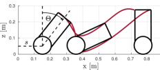
First, let us briefly introduce the TWIPR’s dynamics. We consider a TWIPR moving along a straight line. The motor torque is the input variable and is denoted by $u\in\rm I\!R$. Let $\Theta\in\rm I\!R$ denote the pendulum’s pitch angle and let $s\in\rm I\!R$ denote the robot’s position (see Fig. 3).

Figure 3: The two-wheeled inverted pendulum robot

The state vector $\mathbf{z}\in\rm I\!R^{4}$ is defined as

$$\mathbf{z}=\left[\Theta\hskip 5.69046pt\dot{\Theta}\hskip 5.69046pts\hskip 5.69046pt\dot{s}\right]^{T}\,.$$ (48)

A thorough derivation of the TWIPR’s dynamics can be found in Kim and Kwon (2015). It has been successfully employed elsewhere, see, e.g., Music et al. (2018), whose notation is also employed here. By this, let the dynamics be

$$\forall t\in\rm I\!R_{\geq 0},\qquad\dot{\mathbf{z}}(t)=f\left(\mathbf{z}(t),u(t)\right)\,.$$ (49)

To stabilize the inverted pendulum, the controller input $u_{\mathrm{C}}\in\rm I\!R$ is calculated by a time-discrete feedback controller of the form

$$u_{\mathrm{c}}=-\mathbf{K}\mathbf{z}\,,$$ (50)

with sampling time $T=0.02\ \mathrm{sec}$. The feedback matrix $\mathbf{K}^{1\times 4}$ is designed using pole-placement and the linearised (at the upright equilibrium), discretised form of the dynamics (49).

For demonstration purposes, the reference trajectory

$$r(n)=1.22\rm{sin}\left(2/3\pi Tn\right)$$ (51)

with $N=150$ samples is chosen, whose lifted form is denoted by $\mathbf{r}\in\rm I\!R^{N}$. To perform this trajectory an ILC system is implemented, which calculates the input variable $u_{\mathrm{ILC}}\in\rm I\!R$, which is an additional motor torque leading to the overall input

$$\forall n=1,\dots,N,\quad u(n)=u_{\mathrm{C}}(n)+u_{\mathrm{ILC}}(n)\,.$$ (52)

Figure 4: Block diagram of the ILC system

The lifted form of the ILC’s input variable $u_{\mathrm{ILC}}$ is denoted by $\mathbf{u}_{j}\in\rm I\!R^{N}$, where $j\in\rm I\!N$ denotes the trial index. To update the input trajectory $\mathbf{u}_{j}$, an ILC law as in (5), is applied, where $\mathbf{L}\in\rm I\!R^{N\times N}$ denotes the lifted form of the learning function and $\mathbf{Q}\in\rm I\!R^{N\times N}$ denotes the lifted form of the Q-filter. To design both these transfer functions, the dynamics of the closed loop plant are linearised leading to the lifted form $\mathbf{P}\in\rm I\!R^{N\times N}$ and the linear dynamics (2), where $\mathbf{y}_{j}\in\rm I\!R^{N}$ denotes the pitch trajectory. The learning matrix and Q-filter are calculated using quadratic optimal design, see Bristow et al. (2006), yielding an asymptotically stable, monotonically convergent ILC system with the convergence rates

$$\gamma_{\mathrm{2}}=0.5$$ (53)

and

$$\gamma_{\infty}=0.64\,.$$ (54)

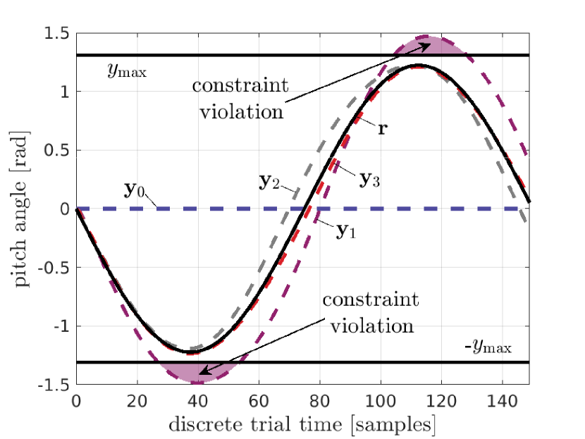
The ILC is output-constrained as, due to the TWIPR’s design, the pitch angle is limited by

$$\forall j\in\rm I\!N_{\mathrm{0}},\quad\left|\left|{\mathbf{y}_{j}}\right|\right|_{\infty}\leq y_{\mathrm{max}}=1.31\ [\mathrm{rad}]\,.$$ (55)

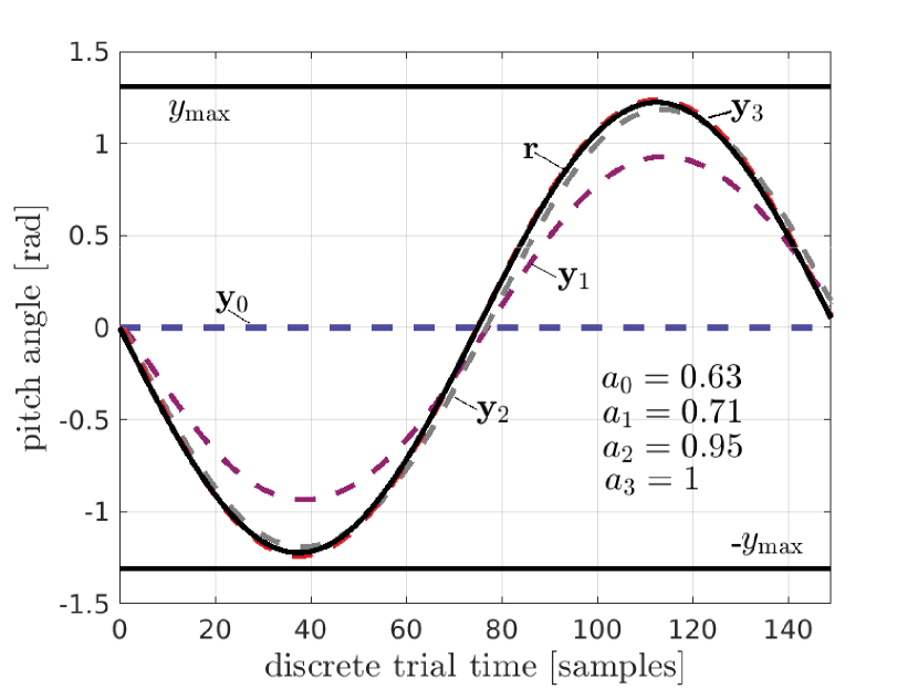
To demonstrate the impact of this restriction, consider the simulation results of applying the conventional ILC system to the TWIPR’s non-linear dynamics, which are displayed in Fig. 4. On the first trial, the output trajectory $\mathbf{y}_{\mathrm{1}}$ violates the constraints characterized by $y_{\mathrm{max}}$.

Figure 5: Output Progression of the conventional ILC

To ensure that the output constraints are not violated, the RAILC algorithm is applied in simulation first. To meet Assumption 1, the initial input trajectory

$$\mathbf{u}_{\mathrm{0}}=\mathbf{0}$$ (56)

is chosen. Assumption 2 is also satisfied as the reference trajectory does not exceed the maximum value. Lastly, the upper bounde estimate $\overline{\epsilon}$ is chosen as

$$\overline{\epsilon}=2\left|\left|{\left(\mathbf{I}-\mathbf{P}\mathbf{Q}\mathbf{P}^{-1}\right)\mathbf{r}}\right|\right|_{\infty}\,.$$ (57)

Results in Fig. 5 show that the RAILC system complies with the output constraints as derived in Proposition 5.

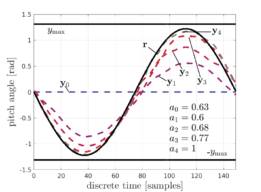
Figure 6: Output Progression of the RAILC in simulation

Afterwards, the RAILC algorithm is experimentally validated using the TWIPR. Fig. 6 illustrates that the RAILC algorithm also complies with the output constraints when applied experimentally.

Figure 7: Experimental Output Progression of the RAILC

Due to (53) and (9), the conventional ILC system is monotonically convergent. As

$$\left|\left|{\mathbf{P}\mathbf{Q}\mathbf{P}^{-1}}\right|\right|_{2}=1$$ (58)

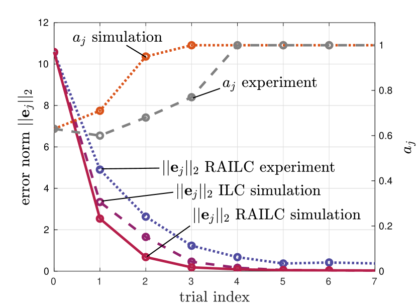
also fulfills the condition of Proposition 7, the RAILC system is monotonically convergent above a threshold under the Euclidean norm. Fig. 7 shows the progression of the error norms and validates this theoretical finding in both simulation and experiment. Furthermore, in simulation, the RAILC achieves a faster decline of the error norm than the conventional ILC system.

Figure 8: Progression of the error norms $\left|\left|{\mathbf{e}_{j}}\right|\right|$ and $a_{j}$

A solution to the reference adaptation problem, as discussed in Proposition 1, has been obtained at every trial, both in simulation and experiment. Fig. 7 shows that, in simulation, the value of $a_{j}$ is monotonically increasing and equals one from the third trial onward. In the experiment, $a_{j}$ is not monotonically increasing as there is a decrease in the first trial. From there onward, $a_{j}$ is monotonically increasing and reaches one on the fourth trial.

7 Conclusion

We have extended standard ILC schemes in a modular fashion to cope with output-constrained systems. By adapting the reference trajectory based on a conservative estimate of the output progression, the violation of output constraints is avoided. Under mild assumptions on disturbances, reference trajectory and the output trajectory, the existence of a solution is guaranteed. A condition for the RAILC error to monotonically converge above a threshold was given. It has been shown that this threshold can be expected to be close to zero. The RAILC approach has been applied to a TWIPR, and both simulation and experimental results have been shown. While the conventional ILC system violates output constraints, the RAILC system complies with them. Furthermore, the RAILC system exhibits monotonic convergence above a small threshold in both simulation and experiment. Finally, simulation results show that applying RAILC does not slow down the decline of the error norm when compared to the conventional ILC.

Ongoing work investigates conditions for the existence of a solution to the optimization problem (22). Furthermore, we will study the possibility of using RAILC to increase performance.

Appendix A Proposition 8

Lemma 1

Given a matrix $\mathbf{A}\in\rm I\!R^{N\times N}$, a matrix $\mathbf{B}\in\rm I\!R^{N\times N}$, and a vector $\mathbf{v}\in\rm I\!R^{N\times N}$ with

$$\left|\left|{\mathbf{v}}\right|\right|_{2}=1\,,$$ (59)

if (sufficient condition)

$$\left|\left|{\mathbf{B}-\mathbf{A}}\right|\right|_{2}<1\,,$$ (60)

then

$$\mathbf{v}^{T}\left(\mathbf{B}^{T}\mathbf{A}+\mathbf{A}^{T}\mathbf{B}\right)\mathbf{v}>\mathbf{v}^{T}\mathbf{A}^{T}\mathbf{A}\mathbf{v}+\mathbf{v}^{T}\mathbf{B}^{T}\mathbf{B}\mathbf{v}-1\,.$$ (61)

Combining (60), (59), and the submultiplicativity of norms gives

$$1>\left|\left|{\mathbf{B}-\mathbf{A}}\right|\right|_{2}=\left|\left|{\mathbf{B}-\mathbf{A}}\right|\right|_{2}\left|\left|{\mathbf{v}}\right|\right|_{2}\\ \geq\left|\left|{\mathbf{B}\mathbf{v}-\mathbf{A}\mathbf{v}}\right|\right|_{2}=\sqrt{{\left(\mathbf{B}\mathbf{v}-\mathbf{A}\mathbf{v}\right)}^{T}\left(\mathbf{B}\mathbf{v}-\mathbf{A}\mathbf{v}\right)}\,,$$ (62)

which, by taking the squares and expanding, leads to (61), thus, concluding the proof.

Proposition 8

Given a matrix $\mathbf{A}\in\rm I\!R^{N\times N}$, a matrix $\mathbf{B}\in\rm I\!R^{N\times N}$, and a scalar $a\in(0,1]$, if (sufficient condition)

$$\left|\left|{\mathbf{B}-\mathbf{A}}\right|\right|_{2}<1\quad\mathit{and}\quad\left|\left|{\mathbf{B}}\right|\right|_{2}\leq 1\,,$$ (63)

then

$$\left|\left|{\mathbf{B}-a\mathbf{A}}\right|\right|_{2}<1\,.$$ (64)

First, let $\mathbf{w}\in\rm I\!R^{N}$ denote a vector such that

$$\mathbf{w}=\underset{\left|\left|{\mathbf{x}}\right|\right|_{2}=1}{\mathrm{argmax}}\left\{\left|\left|{\left(\mathbf{B}-a\mathbf{A}\right)\mathbf{x}}\right|\right|_{2}\right\}\,,$$ (65)

which, according to the definition of induced matrix norms, implies

$$\left|\left|{\mathbf{B}-a\mathbf{A}}\right|\right|_{2}=\left|\left|{\left(\mathbf{B}-a\mathbf{A}\right)\mathbf{w}}\right|\right|_{2}=\\ \sqrt{\mathbf{w}^{T}\mathbf{B}^{T}\mathbf{B}\mathbf{w}-a\mathbf{w}^{T}\left(\mathbf{B}^{T}\mathbf{A}+\mathbf{A}^{T}\mathbf{B}\right)\mathbf{w}+a^{2}\mathbf{w}^{T}\mathbf{A}^{T}\mathbf{A}\mathbf{w}}\,.$$ (66)

Lemma 1 further gives

$$\mathbf{w}^{T}\left(\mathbf{B}^{T}\mathbf{A}+\mathbf{A}^{T}\mathbf{B}\right)\mathbf{w}>\mathbf{w}^{T}\mathbf{A}^{T}\mathbf{A}\mathbf{w}+\mathbf{w}^{T}\mathbf{B}^{T}\mathbf{B}\mathbf{w}-1\,,$$ (67)

which combined with (66) leads to

$$\left|\left|{\mathbf{B}-a\mathbf{A}}\right|\right|_{2}<\\ \sqrt{(1-a)\mathbf{w}^{T}\mathbf{B}^{T}\mathbf{B}\mathbf{w}+a+(a^{2}-a)\mathbf{w}^{T}\mathbf{A}^{T}\mathbf{A}\mathbf{w}}\,.$$ (68)

Submultiplicativity of norms, (63), and (65) give

$$\mathbf{w}^{T}\mathbf{B}^{T}\mathbf{B}\mathbf{w}\leq 1\,,$$ (69)

which combined with

$$a\in(0,1]~{}\implies~{}a^{2}\leq a~{}\implies~{}a^{2}-a\leq 0$$ (70)

and (68) leads to

$$\left|\left|{\mathbf{B}-a\mathbf{A}}\right|\right|_{2}<\sqrt{1-a+a}=1\,.$$ (71)

This concludes the proof.

References

• Bristow et al. (2006) Bristow, D. A., Tharayil, M., Alleyne, A. G., 2006. A survey of iterative learning control. IEEE control systems magazine 26 (3), 96–114.
• Elci et al. (2002) Elci, H., Longman, R. W., Phan, M. Q., Juang, J.-N., Ugoletti, R., Aug 2002. Simple learning control made practical by zero-phase filtering: applications to robotics. IEEE Transactions on Circuits and Systems I: Fundamental Theory and Applications 49 (6), 753–767.
• Jin et al. (2014) Jin, X., Wang, Z., Kwong, R. H., 2014. Convex optimization based iterative learning control for iteration-varying systems under output constraints. In: 11th IEEE International Conference on Control & Automation (ICCA). IEEE, Piscataway, NJ, pp. 1444–1448.
• Kim and Kwon (2015) Kim, S., Kwon, S., 2015. Dynamic modeling of a two-wheeled inverted pendulum balancing mobile robot. International Journal of Control, Automation and Systems 13 (4), 926–933.
• Moore et al. (1992) Moore, K. L., Dahleh, M., Bhattacharyya, S. P., Jul 1992. Iterative learning control: A survey and new results. J. Robotic Syst. 9 (5), 563–594.
• Music et al. (2018) Music, Z., Molinari, F., Gallenmüller, S., Ayan, O., Raisch, J., Nov 2018. Design of a Networked Controller for a Two-Wheeled Inverted Pendulum Robot. ResearchGate.
• Pandit and Buchheit (1999) Pandit, M., Buchheit, K.-H., May 1999. Optimizing iterative learning control of cyclic production processes with application to extruders. IEEE Trans. Control Syst. Technol. 7 (3), 382–390.
• Rogers and Tutty (2016) Rogers, E., Tutty, O. R., Sep 2016. Iterative learning control with applications in energy generation, lasers and health care. Proceedings. Mathematical, Physical, and Engineering Sciences / The Royal Society 472 (2193).
• Sebastian et al. (2018a) Sebastian, G., Tan, Y., Oetomo, D., Mareels, I., 2018a. Feedback-based iterative learning design and synthesis with output constraints for robotic manipulators. IEEE Control Systems Letters 2 (3), 513–518.
• Sebastian et al. (2018b) Sebastian, G., Tan, Y., Oetomo, D., Mareels, I., 2018b. Iterative learning control for linear time-varying systems with input and output constraints. In: The 2018 Australian & New Zealand Control Conference - ANZCC 2018. IEEE, [Piscataway, New Jersey], pp. 87–92.
• Seel et al. (2011) Seel, T., Schauer, T., Raisch, J., Jan 2011. Iterative Learning Control for Variable Pass Length Systems. IFAC Proceedings Volumes 44 (1), 4880–4885.
• Seel et al. (2017) Seel, T., Schauer, T., Raisch, J., Mar 2017. Monotonic convergence of iterative learning control systems with variable pass length. Int. J. Control 90 (3), 393–406.