Automatic structured variational inference
Luca Ambrogioni1 Kate Lin2 Emily Fertig2 Sharad Vikram2
Max Hinne1 Dave Moore2 Marcel van Gerven1
1Department of Artificial Intelligence, Donders Institute for Brain, Cognition and Behaviour Radboud University, Nijmegen, the Netherlands 2Google Research, San Francisco, CA, USA
Abstract
Stochastic variational inference offers an attractive option as a default method for differentiable probabilistic programming. However, the performance of the variational approach depends on the choice of an appropriate variational family. Here, we introduce automatic structured variational inference (ASVI), a fully automated method for constructing structured variational families, inspired by the closed-form update in conjugate Bayesian models. These convex-update families incorporate the forward pass of the input probabilistic program and can therefore capture complex statistical dependencies. Convex-update families have the same space and time complexity as the input probabilistic program and are therefore tractable for a very large family of models including both continuous and discrete variables. We validate our automatic variational method on a wide range of low- and high-dimensional inference problems. We find that ASVI provides a clear improvement in performance when compared with other popular approaches such as the mean-field approach and inverse autoregressive flows. We provide an open source implementation of ASVI in TensorFlow Probability.
1 Introduction
The aim of probabilistic programming is to automate every aspect of probabilistic inference in arbitrary probabilistic models (programs), so that the user can focus her attention on modeling. Stochastic gradient-based variational methods have recently emerged as a powerful alternative to MCMC for inference in differentiable probabilistic programming languages (Wingate and Weber, 2013; Kucukelbir et al., 2017; Tran et al., 2016; Kucukelbir et al., 2015; Bingham et al., 2019). This trend is a consequence of the increasing automatization of variational inference (VI) techniques, which evolved from requiring highly mathematically sophisticated and model-specific tools, to generic algorithms that can be applied to a broad class of problems without model-specific derivations (Hoffman et al., 2013; Kingma and Welling, 2013; Hernández-Lobato and Adams, 2015; Ranganath et al., 2014). However, applications of VI usually require the user to specify a parameterized variational family. In general, it is relatively easy to automate the construction of the variational distribution under a mean-field approximation, where the approximate posterior distribution factorizes as a product of univariate distributions. However, while there is a substantial body of model-specific research on structured variational families, few existing methods can be used for automatically constructing an appropriate scalable structured variational approximation for an arbitrarily chosen probabilistic model. Instead, existing methods either ignore most of the prior structure of the model (e.g. ADVI with the multivariate Gaussian distribution (Kucukelbir et al., 2017)) or require strict assumptions such as local conjugacy (e.g. structured stochastic VI (Hoffman and Blei, 2015)). In addition, several of these methods require the use of ad-hoc gradient estimators or variational lower bounds (Tran et al., 2015; Ranganath et al., 2016).
In this paper we introduce an automatic procedure for constructing variational approximations that incorporate the structure of the probabilistic model, while being flexible enough to capture the distribution of the observed data. The construction of these variational approximations is fully automatic and the resulting variational distribution has the same time and space complexity as the input probabilistic program. The new family of variational models, which we call the convex-update variational family, interpolates the evidence coming from the observed data with the feedforward structure of the model prior. Specifically, the parameters of the posterior distribution of each latent variable are a convex combination of the parameters induced by the parents of that variable, and a term reflecting the influence of the data. This mimics the evidence update in the expectation parameters of conjugate exponential family models, where this posterior is given in closed form. The convex-update variational family can be trained using standard inference techniques and gradient estimators and can therefore be used as a drop-in replacement of the mean-field approach in automatic differentiation stochastic VI. We refer to this new form of fully automatic inference as automatic structured variational inference (ASVI). A full implementation is open-sourced in TensorFlow Probability as tfp.experimental.build_asvi_surrogate_posterior.
2 Preliminaries
VI is used to approximate the posterior over the latent variables of a probabilistic program with a member of a parameterized family of probability distributions . The vector of variational parameters is obtained by maximizing the evidence lower bound (ELBO):
| (1) |
where is a likelihood function. The resulting variational posterior (i.e. the maximum of this optimization problem) depends on the choice of the parameterized family and is equal to the exact posterior only when the latter is included in the family. In this paper we restrict our attention to probabilistic programs that are specified in terms of conditional probabilities and densities chained together by deterministic functions:
| (2) |
where is a family of probability distributions and is a subset of parent variables such that the resulting graphical model is a directed acyclic graph (DAG). The vector-valued functions specify the value of the parameters of the distribution of the latent variable given the values of all its parents.
2.1 Convex updates in conjugate models
Exponential family distributions play a central role in Bayesian statistics as the only families that support conjugate priors, where the posterior is available via an analytic expression (Diaconis and Ylvisaker, 1979). An exponential family distribution can be parameterized by a vector of expectation parameters , where is the vector of sufficient statistics of the data. We can assign to these parameters a conjugate prior distribution , which in turn is parameterized by the prior expectation . Upon observing independently sampled datapoints, under some boundary assumptions, it can be shown that the posterior expectation parameters are a convex combination of the prior parameters and the maximum likelihood estimator (Diaconis and Ylvisaker, 1979):
| (3) |
where is a vector of convex combination coefficients and denotes the element-wise product. A derivation of this result is given in Supplementary Material A.
For example, in a Gaussian model with known precision and a Gaussian prior over the mean, the posterior mean is given by
| (4) |
where is the precision of the prior. This formula shows that the posterior parameters are a trade-off between the prior hyper-parameters and the values induced by the data.
3 Convex-update variational families
"2D\lst@ttfamily–
Consider the following probabilistic model:
| (5) |
where is a likelihood function and is a prior distribution parameterized by a vector of parameters . We do not assume the likelihood or the prior to be in the exponential family; simply that the parameters are defined in a convex domain. We can construct a convex-update parameterized variational family by mimicking the form of the parameter update rule in conjugate models:
| (6) |
where is now a vector of learnable parameters with entries ranging from to and is a vector of learnable parameters with the same range of possible values as . In practice, it is convenient to express each as the logistic sigmoid of a logit parameter, so that we can perform unconstrained optimization in the logit space.
In a model with a single latent variable, the convex-update parameterization is over-parameterized and equivalent to mean field. However, the power of this approach becomes evident in multivariate models constructed by chaining basic probability distributions together. Consider a probabilistic program specified in the form of Eq. (2). We can construct a structured variational family by applying the convex-update form to each latent conditional distribution in the model:
| (7) |
with , and the convex update operator:
| (8) |
The multivariate structured distributions induced by this family have several appealing theoretical properties that justify their usage in structured inference problems:
-
1.
The family always contains the original probabilistic program (i.e. the prior distribution). This is trivial to see as we can obtain the prior by setting . On the other hand, setting results in the standard mean-field approximation. Note that none of the commonly used automatic structured variational approaches share this basic property.
-
2.
The family includes both the exact filtering and smoothing posterior of univariate linear Gaussian time series models of the form
(9) In this case, the filtering conditional posterior is given by the Kalman filter update:
(10) where is the Kalman gain, corresponding to in ASVI. The smoothing update has a similar form where the data term is augmented with an estimate integrating all future observations.
-
3.
The convex-update family has a very parsimonious parameterization compared to other structured families. The number of parameters is , where is the total number of parameters of the conditional distributions. In contrast, the common multivariate normal approach scales as . However, this parsimonious parameterization implies that the convex-update family cannot capture dependencies that are not already present in the prior of the probabilistic program. Specifically, the convex-update family cannot model correlations originating from colliding arrows in the directed acyclic graph (‘explaining away’ dependencies).
4 Discrete latent variables and stochastic control flow
While this paper is focused on differentiable probabilistic programming, the pseudo-conjugate family can be applied equally well to models with discrete latent variables and combinatorial link functions. Consider a conditional Bernoulli variable:
| (11) |
where the array collects the values of its parents. Since the parameter is defined in a convex domain, we can construct a convex-update variational posterior:
| (12) |
It is easy to see that the same procedure can be applied to binomial, categorical, multinomial and Poisson variables among others. Using discrete variables, we can also construct convex-update families with stochastic control flows. For example, a binary latent can determine whether the stochastic computation proceeds on one branch of the computation tree rather than another. This has the nice feature of having an approximate posterior program with the same stochastic flow structure of the prior program where the probability of each gate is biased by the observed data.
5 Automatic structured variational inference
Construction of the variational family (7) can be straightforwardly automated by probabilistic programming systems. A variational program is defined by running the input program under a nonstandard interpretation: at each random variable site
the variational program instead samples from the convex-update distribution (Eq. (6)),
where and are trainable variables. Because each variable definition is rewritten ‘locally’, the variational program has the same control-flow structure, dependence graph, and time complexity as the original model. Local transformations of this kind may be implemented by effect handlers (Plotkin and Pretnar, 2009), a mechanism supported in multiple recent probabilistic programming frameworks (Moore and Gorinova, 2018; Bingham et al., 2019; Phan et al., 2019).
We provide an open-source implementation of ASVI for joint distribution models in TensorFlow Probability (TFP; Dillon et al., 2017), which uses an effect-handling-like mechanism (Python coroutines) to transform an input joint distribution into a structured variational surrogate. Figure 2 shows a simplified version.
Our implementation operates in the default parameterization of each TFP distribution class, which is typically similar (if not exactly equal) to the expectation parameterization; e.g., normal distributions expose a location-scale parameterization. Constrained variational parameters are defined as differentiable transformations of unconstrained variables, where each distribution is annotated with appropriate constraining transformations for its parameters. For example, the softplus transformation enforces that scale parameters have positive values. For variables such as log-normal distributions whose definition involves a bijective transformation of a base variable , the convex-update family has an analogous form and defines a convex update on the union of the parameters .
Given a structured variational program, the ELBO (1) may be estimated by Monte Carlo sampling and optimized with stochastic gradient estimates, obtained via the reparameterization trick for continuous-valued variables and score-function estimator for discrete variables (Ranganath et al., 2014; Kucukelbir et al., 2017).
6 Related work
Most structured VI approaches require model specific derivations and variational bounds. However, several forms of model-agnostic structured variational distributions have been introduced. The most commonly used fully automatic approach is probably automatic differentiation variational inference (ADVI) (Kucukelbir et al., 2017). The ADVI variational family is constructed by mapping the values of all latent variables to an unbounded coordinate space based on the support of each distribution. The variational distribution in this new space is then parameterized as either a spherical (mean field) or a fully multivariate normal distribution. While this approach is broadly applicable, it exploits very little information from the original probabilistic model and has scalability problems due to the cubic complexity of Bayesian inference when the multivariate distribution is used. Hierarchical VI accounts for dependencies between latent variables by coupling the parameters of their factorized distributions through a joint variational prior (Ranganath et al., 2016). While this method is very generic, it requires user input in order to define the variational prior and it uses a modified variational lower bound. Copula VI models the dependencies between latent variables using a vine copula function (Tran et al., 2015). In the context of probabilistic programming, copula VI shares some of the same limitations of hierarchical VI: it requires the appropriate specification of bivariate copulas and it needs a specialized inference technique. The approach that is closest to our current work is structured stochastic VI (Hoffman et al., 2013). Similar to our approach, its variational posteriors have the same conditional independence structure as the input probabilistic program. However, this method is limited to conditionally conjugate models with exponential family distributions. Furthermore, the resulting ELBO is intractable and needs to be estimated using specialized techniques. Similarly, conjugate-Computation Variational Inference uses conjugate Bayesian updates in non-conjugate models with locally conjugate components (Khan and Lin, 2017). This differs from our approach as we use the convex updates for all the variables in the model.
Normalizing flows are general deep learning methods designed to approximate arbitrary probability densities through a series of learnable invertible mappings with tractable Jacobians (Rezende and Mohamed, 2015; Kingma et al., 2016; Dinh et al., 2016; Kingma and Dhariwal, 2018; Papamakarios et al., 2017; Kobyzev et al., 2020). Flows have been used in stochastic VI as very expressive and highly parameterized variational families (Rezende and Mohamed, 2015; Kingma et al., 2016). Most normalizing flow architectures used in VI do not incorporate the conditional independence structure of the prior probabilistic program. Structured conditional continuous normalizing flows are a new class of normalizing flows that have the conditional independence structure of the true posterior (Weilbach et al., 2020). These architectures are based on faithful inversion (Webb et al., 2018) and implement the dependency structure using sparse matrices. Conversely to ASVI, this approach only exploits the graphical structure of the probabilistic program and therefore ignores the specific form of the conditional distributions and link functions.
Structured VI is most commonly applied in time series models such as hidden Markov models and autoregressive models. In these cases the posterior distributions inherit strong statistical dependencies from the sequential nature of the prior. Structured VI for time series usually use structured variational families that capture the temporal dependencies, while being fully-factorized in the non-temporal variables (Eddy, 1996; Foti et al., 2014; Johnson and Willsky, 2014; Karl et al., 2016; Fortunato et al., 2017). This differs from our convex-update families, where both temporal and non-temporal dependencies are preserved.
7 Applications
We first evaluate ASVI on a set of standardized Bayesian inference tasks to compare ASVI to other automated inference methods. We then apply ASVI to a both a deep Bayesian smoothing and a deep generative modeling task, to demonstrate that ASVI scales to large datasets while producing high quality posteriors. The code needed to run ASVI and baselines on the standardized tasks can be found in this repository.
7.1 Inference Gym tasks
| ASVI | Mean field | Small IAF | Large IAF | MVN | AR(1) | |
|---|---|---|---|---|---|---|
| BR | ||||||
| BRG | ||||||
| LZ | ||||||
| LZG | ||||||
| ES | N/A | |||||
| R | N/A |
| ASVI | Mean field | Small IAF | Large IAF | MVN | AR(1) | ||
|---|---|---|---|---|---|---|---|
| BR | M | ||||||
| SD | |||||||
| BRG | M | ||||||
| SD | |||||||
| LZ | M | ||||||
| SD | |||||||
| LZG | M | ||||||
| SD | |||||||
| ES | M | N/A | |||||
| SD | N/A | ||||||
| R | M | N/A | |||||
| SD | N/A |
Inference Gym (IG; Sountsov et al., 2020) is a Python library for evaluating probabilistic inference algorithms. It defines a set of standardized inference tasks and provides implementations as TFP joint distribution models (Piponi et al., 2020) and as Stan programs (Carpenter et al., 2017), which are used to compute ‘ground truth’ posterior statistics via MCMC.
For each task we evaluate ASVI against a suite of baseline variational posteriors, including mean field (MF), inverse autoregressive flows (Kingma et al., 2016; Papamakarios et al., 2017) with eight hidden units (Small IAF) and 512 hidden units (Large IAF), and a multivariate normal posterior (MVN). Where possible, we also compare to an AR(1) posterior. For each method the ELBO is optimized to convergence (up to 100000 steps, although significantly fewer were required in most cases) using the Adam optimizer, with learning rate set by a hyperparameter sweep for each task/method pair—this tuning was particularly important for the IAF models. Further details are provided in the supplement.
Time series. We consider two discretized stochastic differential equation (SDE) models, defined by conditional densities of the following form:
| (13) | ||||
| (14) |
where represents the latent process with drift function and volatility function , and observations are taken with noise standard deviation . The first model describes Brownian (BR) motion without drift, and the second model is a stochastic Lorenz dynamical system (LZ). Full model specifications are provided in the supplementary material. We also include variants of both models that include global variables (BRG and LZG) where the innovation and observation noise scale parameters are unknown. We simulate each model forward 30 steps and assume that noisy observations are taken of the first ten and last ten steps, and the middle ten are unobserved.
Hierarchical regression models. We also evaluate ASVI on two standard Bayesian hierarchical models: Eight Schools (ES; Gelman et al., 2013), which models the effect of coaching programs on standardized test scores, and Radon (R; Gelman and Hill, 2007), a hierarchical linear regression model that predicts Radon measurements taken in houses. Full descriptions are provided in the supplementary material.
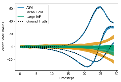
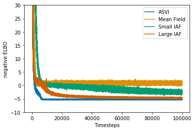
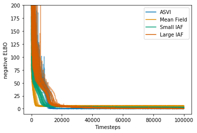
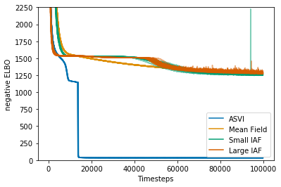
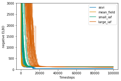
Results. Table 1 shows that ASVI and the large IAF produce the best ELBOs; ASVI is competitive with the large IAF on all tasks despite having far fewer parameters. Similarly, in Table 2 we see that ASVI’s estimates of posterior means and standard deviations are consistently among the best relative to MCMC ground truth. Mean field fails to converge to the true posterior estimate in all four models, indicating that inclusion of prior structure in ASVI is needed to capture the dependencies in the true posterior. Qualitatively, we observe in Figure 3 that only the ASVI posterior captures the ground truth posterior in the Lorenz task, indicating that ASVI is able to capitalize on strong prior structure when it exists. Figure 1 in the supplementary material shows loss trajectories. For all but the Radon model, ASVI tends to converge in fewer iterations than the large IAF, the other highest-performing surrogate posterior.
7.2 Deep Bayesian smoothing with neural SDEs
So far, we performed inference in simple time series and hierarchical models with relatively low-dimensional state spaces. We will now test the performance of ASVI on a high-dimensional problem with complex nonlinearities parameterized by deep networks. As a latent model, we use neural (discretized) stochastic differential equations (SDE) (Chen et al., 2018; Li et al., 2020):
| (15) |
where is a nonlinear function parameterized by a neural network and is standard multivariate Brownian motion (see Supplementary Material C for the details of the architecture). This latent process generates noise-corrupted observations through a deep network :
| (16) |
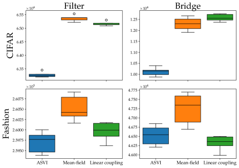
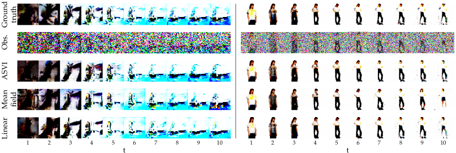
In our examples, is a generator which converts latent vectors into RGB images. We tested two kinds of pre-trained generators: A DCGAN trained on CIFAR10 and a DCGAN trained on FashionGEN (Radford et al., 2015) (see Supplementary Material C). In the former case, the latent space is -dimensional, while in the latter it is -dimensional. We considered two inference challenges: filtering, where we aim to remove the noise from a series of images generated by a trajectory in the latent process, and bridging, where we reconstruct a series of intermediate observations given the beginning (first three time points) and the end (last two time points) of a trajectory. In both cases, we assume knowledge of the dynamical and generative models, discretize the neural SDE using an Euler–Maruyama scheme and backpropagate through the integrator (Chen et al., 2018).
Figure 5 shows the filtering performance of ASVI and two baselines (mean field, and linear Gaussian model; see Supplementary Material C for the details) in a bridging problem. The quantitative results (negative ELBOs) are shown in Figure 4. ASVI always reaches tighter lower bounds except in the Fashion bridge experiment where it has slightly lower performance than the linear coupling baseline. This tighter variational bound results in discernibly higher quality filtered images in both CIFAR10 and Fashion, as shown in Figure 5. The figure also shows several samples from the ASVI bridge posterior. As expected, the generated images diverge in the unobserved period and reconverge at the end.
7.3 Deep amortized generative modeling
| MNIST | kMNIST | fMNIST | ||||
|---|---|---|---|---|---|---|
| no labels | labels | no labels | labels | no labels | labels | |
| ASVI | ||||||
| MF | ||||||
Finally, we apply an amortized form of ASVI to a deep generative modeling problem. The goal is to model the joint distribution of a set of binary images paired with class labels . We use a deep variational autoencoder with three layers of latent variables , and coupled in a feed-forward fashion through ReLU fully-connected networks:
| (17) |
where and are fully-connected two-layer networks with ReLU activations, linear output units, and and hidden units respectively, while and are linear layers. The amortized convex-update distribution has the following form:
| (18) |
where the mean vectors are the activation of the -th layer (post ReLU) of a fully-connected 6-layer ReLU inference network (with layer sizes ) that takes the image as input. The scale parameter vectors were obtained by connecting a linear layer to the -th layer, followed by a softplus transformation. The details of all architectures are given in Supplementary Material D. The amortized family was parameterized by and the weights and biases of the inference network. Note that this amortization scheme is not fully automatic as it require the choice of the inference networks. The mean-field baseline had the same form given in Eq. (18), but with the expectation of the distribution fully determined by . We did not include a comparison with the other baselines as it is computationally unfeasible in this larger scale experiment.
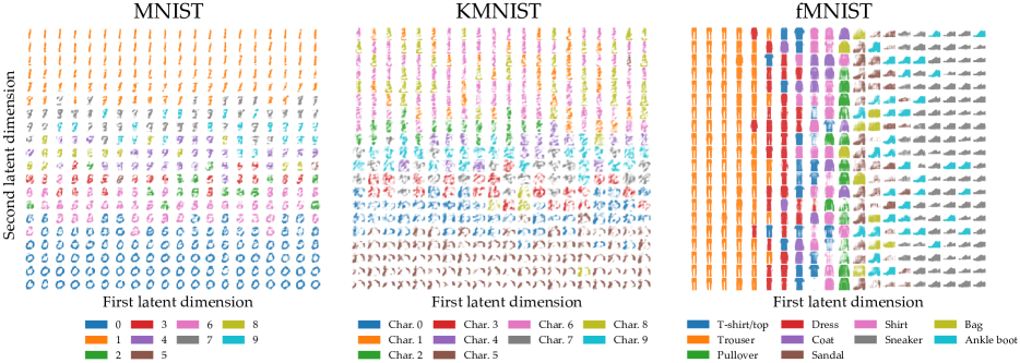
We tested the performance of these deep variational generative models on three computer vision datasets: MNIST, FashionMNIST and KMNIST (LeCun et al., 1998; Xiao et al., 2017; Clanuwat et al., 2018). Furthermore, we performed two types of experiment. In the first, images and labels were generated jointly. In the second, only images were generated. Table 3 reports the performance of ASVI and mean-field baseline quantified as the test set ELBO. The ELBO was estimated by sampling the latent variables times per test image from the variational posterior. Mean ELBO and SEM were obtained by repeating the estimation times. ASVI achieves higher performance in all experiments for all datasets. Figure 6 shows a randomized selection of images generated by the ASVI model together with the corresponding label.
8 Discussion
We introduced an automatic algorithm for constructing an appropriately structured variational family, given an input probabilistic program. The resulting method can be used on any probabilistic program specified by a directed Bayesian network, and always preserves the forward-pass structure of the input program. The main limitation of the convex-update family is that it cannot capture dependencies induced by colliding arrows in the input graphical model. Consequently, in a model such as a standard Bayesian neural network, where the prior over the weights is decoupled, the convex-update family is a mean-field family. Despite this limitation, our results demonstrate good performance (competitive with a high-capacity IAF) on small Bayesian hierarchical models with colliding arrows in the prior graphical model, through capturing the forward structure alone. Designing structured surrogates that efficiently capture the full posterior dependence structure is an interesting direction for ongoing work.
References
- Wingate and Weber (2013) D. Wingate and T. Weber. Automated variational inference in probabilistic programming. ArXiv preprint arXiv:1301.1299, 2013.
- Kucukelbir et al. (2017) A. Kucukelbir, D. Tran, R. Ranganath, A. Gelman, and D. M. Blei. Automatic differentiation variational inference. The Journal of Machine Learning Research, 18(1):430–474, 2017.
- Tran et al. (2016) D. Tran, A. Kucukelbir, A. B Dieng, M. Rudolph, D. Liang, and D. M. Blei. Edward: A library for probabilistic modeling, inference, and criticism. ArXiv preprint arXiv:1610.09787, 2016.
- Kucukelbir et al. (2015) A. Kucukelbir, R. Ranganath, A. Gelman, and D. Blei. Automatic variational inference in Stan. In Advances in Neural Information Processing Systems, 2015.
- Bingham et al. (2019) E. Bingham, J. P. Chen, M. Jankowiak, F. Obermeyer, N. Pradhan, T. Karaletsos, R. Singh, P. Szerlip, P. Horsfall, and N. D. Goodman. Pyro: Deep universal probabilistic programming. The Journal of Machine Learning Research, 20(1):973–978, 2019.
- Hoffman et al. (2013) M. D. Hoffman, D. M. Blei, C. Wang, and J. Paisley. Stochastic variational inference. The Journal of Machine Learning Research, 14(1):1303–1347, 2013.
- Kingma and Welling (2013) D. P. Kingma and M. Welling. Auto-encoding variational Bayes. ArXiv preprint arXiv:1312.6114, 2013.
- Hernández-Lobato and Adams (2015) J. M. Hernández-Lobato and R. Adams. Probabilistic backpropagation for scalable learning of Bayesian neural networks. In International Conference on Machine Learning, pages 1861–1869, 2015.
- Ranganath et al. (2014) R. Ranganath, S. Gerrish, and D. Blei. Black box variational inference. In International Conference on Artificial Intelligence and Statistics, 2014.
- Hoffman and Blei (2015) M. Hoffman and D. Blei. Stochastic structured variational inference. In International Conference on Artificial Intelligence and Statistics, 2015.
- Tran et al. (2015) D. Tran, D. Blei, and E. M. Airoldi. Copula variational inference. In Advances in Neural Information Processing Systems, 2015.
- Ranganath et al. (2016) R. Ranganath, D. Tran, and D. Blei. Hierarchical variational models. In International Conference on Machine Learning, 2016.
- Diaconis and Ylvisaker (1979) P. Diaconis and D. Ylvisaker. Conjugate priors for exponential families. The Annals of Statistics, 7(2):269–281, 1979.
- Plotkin and Pretnar (2009) G. Plotkin and M. Pretnar. Handlers of algebraic effects. In European Symposium on Programming. Springer, 2009.
- Moore and Gorinova (2018) D. Moore and M. I. Gorinova. Effect handling for composable program transformations in Edward2. arXiv preprint arXiv:1811.06150, 2018.
- Phan et al. (2019) D. Phan, N. Pradhan, and M. Jankowiak. Composable effects for flexible and accelerated probabilistic programming in NumPyro. ArXiv preprint arXiv:1912.11554, 2019.
- Dillon et al. (2017) J. V Dillon, I. Langmore, D. Tran, E. Brevdo, S. Vasudevan, D. Moore, B. Patton, A. Alemi, M. Hoffman, and R. A. Saurous. Tensorflow distributions. ArXiv preprint arXiv:1711.10604, 2017.
- Khan and Lin (2017) M. E. Khan and W. Lin. Conjugate-computation variational inference: Converting variational inference in non-conjugate models to inferences in conjugate models. In International Conference on Artificial Intelligence and Statistics, 2017.
- Rezende and Mohamed (2015) D. J. Rezende and S. Mohamed. Variational inference with normalizing flows. In International Conference on Machine Learning, 2015.
- Kingma et al. (2016) D. P Kingma, T. Salimans, R. Jozefowicz, X. Chen, I. Sutskever, and M. Welling. Improved variational inference with inverse autoregressive flow. In Advances in Neural Information Processing Systems, 2016.
- Dinh et al. (2016) L. Dinh, J. Sohl-Dickstein, and S. Bengio. Density estimation using real NVP. arXiv preprint arXiv:1605.08803, 2016.
- Kingma and Dhariwal (2018) D. P. Kingma and P. Dhariwal. Glow: Generative flow with invertible 1x1 convolutions. In Advances in Neural Information Processing Systems, 2018.
- Papamakarios et al. (2017) G. Papamakarios, T. Pavlakou, and I. Murray. Masked autoregressive flow for density estimation. In Advances in Neural Information Processing Systems, 2017.
- Kobyzev et al. (2020) I. Kobyzev, S. Prince, and M. Brubaker. Normalizing flows: An introduction and review of current methods. IEEE Transactions on Pattern Analysis and Machine Intelligence, 2020.
- Weilbach et al. (2020) C. Weilbach, B. Beronov, F. Wood, and W. Harvey. Structured conditional continuous normalizing flows for efficient amortized inference in graphical models. In International Conference on Artificial Intelligence and Statistics, 2020.
- Webb et al. (2018) S. Webb, A. Golinski, R. Zinkov, N. Siddharth, T. Rainforth, Y. W. Teh, and F. Wood. Faithful inversion of generative models for effective amortized inference. In Advances in Neural Information Processing Systems, 2018.
- Eddy (1996) S. R. Eddy. Hidden Markov models. Current Opinion in Structural Biology, 6(3):361–365, 1996.
- Foti et al. (2014) N. Foti, J. Xu, D. Laird, and E. Fox. Stochastic variational inference for hidden Markov models. In Advances in Neural Information Processing Systems, 2014.
- Johnson and Willsky (2014) M. Johnson and A. Willsky. Stochastic variational inference for Bayesian time series models. In International Conference on Machine Learning, 2014.
- Karl et al. (2016) M. Karl, M. Soelch, Ju. Bayer, and P. van der Smagt. Deep variational Bayes filters: Unsupervised learning of state space models from raw data. arXiv preprint arXiv:1605.06432, 2016.
- Fortunato et al. (2017) M. Fortunato, C. Blundell, and O. Vinyals. Bayesian recurrent neural networks. arXiv preprint arXiv:1704.02798, 2017.
- Sountsov et al. (2020) P. Sountsov, A. Radul, and contributors. Inference gym, 2020.
- Piponi et al. (2020) D. Piponi, D. Moore, and J. V. Dillon. Joint distributions for TensorFlow Probability. ArXiv preprint arXiv:2001.11819, 2020.
- Carpenter et al. (2017) B. Carpenter, A. Gelman, M. D. Hoffman, D. Lee, B. Goodrich, M. Betancourt, M. Brubaker, J. Guo, P. Li, and A. Riddell. Stan: A probabilistic programming language. Journal of Statistical Software, 76(1), 2017.
- Gelman et al. (2013) A. Gelman, J. B. Carlin, H. S. Stern, D. B. Dunson, A. Vehtari, and D. B. Rubin. Bayesian Data Analysis. CRC Press, 3rd edition, 2013.
- Gelman and Hill (2007) A. Gelman and J. Hill. Data Analysis using Regression and Multilevel/Hierarchical Models. Cambridge University Press, 2007.
- Chen et al. (2018) T. Q. Chen, Y. Rubanova, J. Bettencourt, and D. K. Duvenaud. Neural ordinary differential equations. In Advances in Neural Information Processing Systems, 2018.
- Li et al. (2020) X. Li, T. L. Wong, R. T.Q. Chen, and D. Duvenaud. Scalable gradients for stochastic differential equations. arXiv preprint arXiv:2001.01328, 2020.
- Radford et al. (2015) A. Radford, L. Metz, and S. Chintala. Unsupervised representation learning with deep convolutional generative adversarial networks. ArXiv preprint arXiv:1511.06434, 2015.
- LeCun et al. (1998) Y. LeCun, L. Bottou, Y. Bengio, and P. Haffner. Gradient-based learning applied to document recognition. Proceedings of the IEEE, 86(11):2278–2324, 1998.
- Xiao et al. (2017) H. Xiao, K. Rasul, and R. Vollgraf. Fashion-MNIST: a novel image dataset for benchmarking machine learning algorithms. arXiv preprint arXiv:1708.07747, 2017.
- Clanuwat et al. (2018) T. Clanuwat, M. Bober-Irizar, A. Kitamoto, A. Lamb, K. Yamamoto, and D. Ha. Deep learning for classical Japanese literature. ArXiv preprint arXiv:1812.01718, 2018.
Appendix A Convex updates in conjugate models
Consider an exponential family likelihood and its expectation parameter:
| (19) |
where is the natural parameter. The conjugate prior is
| (20) |
where is a base density, is the relevant prior natural parameter and is the natural "prior count" parameter. This also induces a prior over the expectation parameters . In Section 2.1, we parameterize this prior using the prior expectations of the expectation parameters
| (21) |
The result in Eq. 3 follows from the fact that . To see this, we can integrate both sides of the trivial identity:
| (22) |
and notice that . This result can be proven when vanishes at the boundary values of the integral using the generalized divergence theorem (Diaconis, 1979). Using this result, we can use the conjugate update rules and to obtain
| (23) | ||||
| (24) | ||||
| (25) |
where is the number of datapoints and can be shown to be the maximum likelihood estimator of the expectation parameter.
Appendix B Details of the Inference Gym experiments
B.1 Inference Gym tasks
Time series models
As a first application, we focus on timeseries models and SDEs. We used two models, both from the Inference Gym (Sountsov et al., 2020).
The first model (BR) is a Brownian motion without drift, governed by , where is a Gaussian white noise process with scale . The value of is observed with noise standard deviation equal to . The data are generated with and . In the BRG model with global variables, both and are treated as random variables with LogNormal(loc=0, scale=2) priors.
The second model (LZ) is a stochastic Lorenz system (nonlinear SDE):
| (26a) | ||||
| (26b) | ||||
| (26c) | ||||
where , and are Gaussian white noise processes with standard deviation . The value of is observed with Gaussian noise with standard deviation ; and are left unobserved. When global variables are allowed (the LZG model), and are treated as unknown random variables with LogNormal(loc=-1., scale=1.) priors.
All processes were discretized with the Euler–Maruyama method ( for BR and for LZ) and the transition probability was approximated as Gaussian (this approximation is exact for tending to ). Each model was integrated for steps.
Hierarchical models
Eight Schools (Gelman et al., 2013) models the effect of coaching programs on standardized test scores, and is specified as follows:
| (27) | ||||
| (28) | ||||
| (29) | ||||
| (30) |
where indexes the schools, represents the prior average treatment effect and controls the variance between schools. The and are observed.
The Radon model (Gelman and Hill, 2007) is a Bayesian hierarchical linear regression model that predicts measurements of Radon, a carcinogenic gas, taken in houses in the United States. The hierarchical structure is reflected in the grouping of houses by county, and the model is specified as follows:
| (31) | ||||
| (32) | ||||
| (33) | ||||
| (34) | ||||
| (35) | ||||
| (36) |
where is the effect for county (with prior mean and standard deviation ) and the are regression coefficients. The log Radon measurement in house , , depends on the effect for the county to which the house belongs, as well as features (the log uranium measurement in county ), (the floor of the house on which the measurement was taken), and (the mean floor by county, a contextual effect). indicates a Normal distribution with mean and variance , truncated to nonnegative values.
B.2 Baselines
Mean Field ADVI
The ADVI (MF) surrogate posterior is constructed with the same procedure as the ASVI posterior, but using only the parameters, or equivalently, fixing . As with ASVI, therefore, the surrogate posterior for each variable is in the same distribution family as its prior. This differs slightly from Kucukelbir et al. (2017), in which surrogate posteriors are always bijectively transformed normal distributions, although we have no reason to believe that this difference is material to our experiments.
Inverse Autoregressive Flows
Inverse Autoregressive Flows (IAFs) are normalizing flows which autoregressively transform a base distribution (Kingma et al., 2016) with a masked neural network (Papamakarios et al., 2017). We build an IAF posterior by transforming a standard Normal distribution with two sequential two-layer IAFs built with tfp.bijectors.MaskedAutoregressiveFlow. The output of the flow is split and restructured to mirror the support of the prior distribution, and then constrained to the support of the prior (for example, by applying a sigmoid transformation to constrain values between zero and one, or a softplus to constrain values to be positive). In our experiments, we use two different-sized IAF posteriors: the “Large” IAF has 512 hidden units in each layer and the “Small” IAF has 8 hidden units in each layer.
Multivariate Normal
The MVN surrogate posterior is built by defining a full-covariance Multivariate Normal distribution with trainable mean and covariance, restructuring the support to the support of the prior, and constraining the samples to the prior support if necessary.
AR(1)
The autoregressive model surrogate learns a linear Gaussian conditional between each pair of successive model variables:
where each and parameterize a learned linear transformation, and is a learned diagonal variance matrix. The linear Gaussian autoregression operates on unconstrained values, which may then be then pushed through constraining transformations as required by the model. To stabilize the optimization, we omit direct dependence on global variables, i.e., when is a global variable we fix (these are generally the first few variables sampled in each model).
B.3 Training details
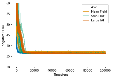
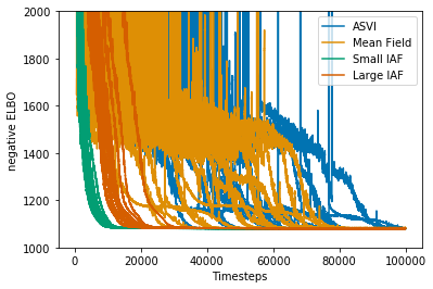
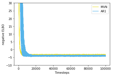
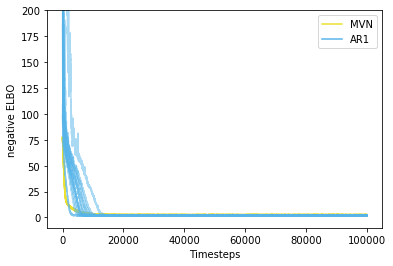
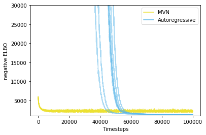
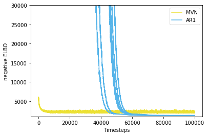
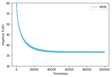
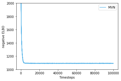
For each of the following inference tasks and posterior baselines, we fit a posterior using full-batch gradient descent on a 1-sample Monte Carlo estimate of the ELBO. We use the Adam optimizer with a learning rates selected by hyperparameter sweep: 1e-2 learning rate for ASVI, MF, and AR(1), 1e-3 for the MVN and Small IAF, and 5e-5 for the Large IAF. Each posterior was trained for 100000 iterations; in Figure 7 and Figure 8, we report the training curves for each posterior-task pair. We find that ASVI successfully converges in all tasks; in most cases, ASVI converges well before 100000 iterations, while MF, Large IAF, and Small IAF fail to converge to a good solution in a few of the tasks.
Appendix C Details of the neural SDE experiment
C.1 Models
The function had the following form
| (37) |
where and were matrices whose entries were sampled in each of the repetitions from a centered normal with SD equal to . Those matrices encodes the forward dynamical model and they were assumed to be known during the experiment. This is a Kalman filter-like setting where the form of the forward model is known and the inference is performed in the latent units. The neural SDE was integrated using Euler–Maruyama integration with step size equal to from to . We trained the model by back-propagating though the integrator.
We used two DCGAN generators as emission models. The networks were the DCGAN implemented in PyTorch. In the CIFAR experiment, we used the following architecture:
The network pretrained on CIFAR was obtained from the GitHub repository: csinva/gan-pretrained-pytorch. The FashionGEN network was downloaded from the pytorch GAN zoo repository. The architectural details are given in Radford et al. (2015).
C.2 Baselines
The ADVI (MF) baseline was obtained by replacing all the conditional Gaussian distributions in the probabilistic program with Gaussian distributions with uncoupled trainable mean and standard deviation parameters. ADVI (MN) was not computationally feasible in this larger scale experiment. Therefore, we implemented a a linear Gaussian model whith conditional densities:
| (38) |
where the matrix , and the vectors and are learnable parameters.
Appendix D Details of the autoencoder experiment
We used the following architectures in our deep autoencoder experiments.
Decoder 1 ()
Decoder 2 ()
Decoder 3 ()
Decoder 4 ()
Inference network ()