Optimal Transport Based Seismic Inversion: Beyond Cycle Skipping

Abstract

Full-waveform inversion (FWI) is today a standard process for the inverse problem of seismic imaging. PDE-constrained optimization is used to determine unknown parameters in a wave equation that represent geophysical properties. The objective function measures the misfit between the observed data and the calculated synthetic data, and it has traditionally been the least-squares norm. In a sequence of papers, we introduced the Wasserstein metric from optimal transport as an alternative misfit function for mitigating the so-called cycle skipping, which is the trapping of the optimization process in local minima. In this paper, we first give a sharper theorem regarding the convexity of the Wasserstein metric as the objective function. We then focus on two new issues. One is the necessary normalization of turning seismic signals into probability measures such that the theory of optimal transport applies. The other, which is beyond cycle skipping, is the inversion for parameters below reflecting interfaces. For the first, we propose a class of normalizations and prove several favorable properties for this class. For the latter, we demonstrate that FWI using optimal transport can recover geophysical properties from domains where no seismic waves travel through. We finally illustrate these properties by the realistic application of imaging salt inclusions, which has been a significant challenge in exploration geophysics.

1 Introduction

The goal in seismic exploration is to estimate essential geophysical properties, most commonly the wave velocity, based on the observed data. The development of human-made seismic sources and advanced recording devices facilitate seismic inversion using entire wavefields in time and space rather than merely travel time information as in classical seismology. The computational technique full-waveform inversion (FWI) [26, 53] was a breakthrough in seismic imaging, and it follows the established strategy of a partial differential equation (PDE) constrained optimization. FWI can achieve results with stunning clarity and resolution [59]. Unknown parameters in a wave equation representing geophysical properties are determined by minimizing the misfit between the observed and PDE-simulated data, i.e.,

$$m^{*}=\operatorname*{argmin}\limits_{m}\{J(f(m),g)+\mathscr{R}(m)\},$$ (1)

where $m$ is the model parameter, which can be seen as a function or discrete as a vector. The misfit $J$ is the objective function, $f(m)$ is the PDE-simulated data given model parameter $m$, $g$ is the observed data, and $\mathscr{R}(m)$ represents the added regularization. In both time [53] and frequency domain [44], the least-squares norm $J(f,g)=||f-g||^{2}_{2}$ has been the most widely used misfit function, which we will hereafter denote as $L^{2}$. In this paper, we focus on the effects of a different choice of the objective function $J$ and avoid adding any regularization $\mathscr{R}(m)$. This is to focus on the properties of the misfit function.

(a) Observed data $g$

(b) Synthetic data $f$

(c) The difference $f-g$

(d) Comparison of the traces at $x=3\,$km

Figure 1: (a) The observed data $g$; (b) the synthetic data $f$; (c) the difference $f-g$; (d) the comparison between two traces at $x=3\,$km, i.e., $f(3,t)$ and $g(3,t)$. Inversion using the $L^{2}$ norm suffers from cycle-skipping issues in this scenario, which is further discussed in Section 6.2.

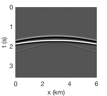
It is, however, well known that FWI based on the $L^{2}$ norm is sensitive to the initial model, the data spectrum, and the noise in the measurement [60]. Cycle skipping can occur when the phase mismatch between the two wave-like signals is greater than half of the wavelength. The fastest way to decrease the $L^{2}$ norm is to match the next cycle instead of the current one, which can lead to an incorrectly updated model parameter. It is a dominant type of local-minima trapping in seismic inversion due to the oscillatory nature of the seismic waves. For example, Figure 1a and Figure 1b show two datasets, which are 2D wavefields measured at the upper boundary. Their phase mismatch is about one wavelength; see Figure 1c and Figure 1d. $L^{2}$-based inversion for this case suffers from cycle-skipping issues. We will discuss inversions based on this example in Section 6.2. When the velocity in the model is too slow compared to the true value, the simulated signal will arrive later than the observed true signal. It is, therefore, natural to study the effects on the mismatch from shifts between the signals.

(a) 2nd order derivative of Gaussian

(b) 4th order derivative of Gaussian

(c) $L^{2}$ misfit

(d) $W_{2}$ misfit

(e) $L^{2}$ misfit

(f) $W_{2}$ misfit

Figure 2: (a) Ricker wavelet $f(t)$ and its shift $f(t-s)$; (b) signal $g(t)$ and its shift $g(t-s)$; (c) the $L^{2}$ norm and (d) the $W_{2}$ distance between $f(t)$ and $f(t-s)$ in terms of shift $s$; (e) the $L^{2}$ norm and (f) the $W_{2}$ distance between $g(t)$ and $g(t-s)$ as a function of $s$. The exponential scaling (3) is applied to normalize the signals for the $W_{2}$ computation; see Section 4.

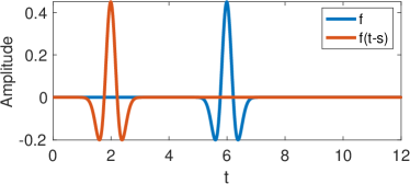
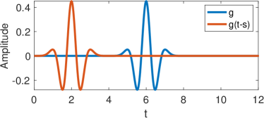
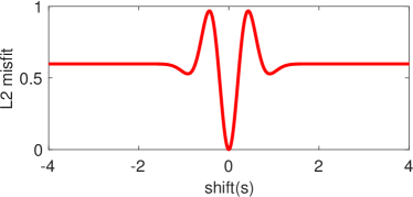
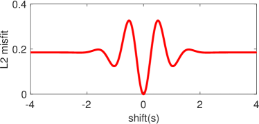
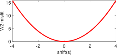
The quadratic Wasserstein distance ($W_{2}$) is ideal for dealing with this type of problem as it has perfect convexity with respect to translation and dilation (Theorem 3.1). We will prove the theorem in Section 3 in a new and more general form. The convexity was the original motivation for us to introduce the Wasserstein distance as the misfit function in seismic inversion [12, 13], which has now been picked up and developed in parallel by many other research groups and generalized to other Wasserstein metric beyond $W_{2}$ [36, 37, 9, 52]. Figure 2 is an illustration of the convexity of the $W_{2}$ metric regarding data translation. The signals used in this example are the Ricker wavelet [49] and the more oscillatory fourth-order derivative of Gaussian. The $W_{2}$ metric precisely captures the data shift $s$ as the misfit is $s^{2}$ independent of the profile of the signal. It is not the case for the $L^{2}$ norm whose basin of attraction depends on the spectral property of the signal.

Although the original goal of introducing optimal transport was to mitigate cycle skipping as discussed above, we will see in this paper that there are other good properties beyond reducing cycle skipping. These properties will be divided into two parts. The first is the effect of data normalization [17], which is an essential preprocessing step of transforming seismic signals to probability densities. In optimal transport theory, there are two main requirements for functions $f$ and $g$ that are compactly supported on a domain $\Pi$:

$$f\geq 0,\quad g\geq 0,\quad<f>\ =\int_{\Pi}f=\int_{\Pi}g=\ <g>.$$

Since these constraints are not expected for seismic signals, different approaches have been promoted to tackle this issue. There exists a significant amount of work from the applied mathematics community to generalize optimal transport to the so-called unbalanced optimal transport [67, 18, 10]. Regarding the non-positivity, the Kantorovich-Rubinstein norm was proposed to approximate the 1-Wasserstein metric [36] and mapping seismic signals into a graph space by increasing the dimensionality of the optimal transport problem by one is also demonstrated to be a feasible solution [34, 35].

Another way to achieve data positivity and mass conservation is to directly transform the seismic data into probability densities by linear or nonlinear scaling functions [46, 17, 16, 66]. In this paper, we focus on the fundamental properties of such data normalizations on $W_{2}$-based inversion. In [66], we normalized the signals by adding a constant and then scaling:

$$\tilde{f}=\frac{f+b}{<f+b>},\quad\tilde{g}=\frac{g+b}{<g+b>},\quad b>0.$$ (2)

An exponential based normalization (Equation (3)) was proposed in [46]. Later, the softplus function defined in Equation (4) [20] as a more stable version of the exponential scaling, soon became popular in practice.

$$\tilde{f}=\frac{\exp(bf)}{<\exp(bf)>},\quad\tilde{g}=\frac{\exp(bg)}{<\exp(bg)>},\quad b>0.$$ (3)

$$\tilde{f}=\frac{\log(\exp(bf)+1)}{<\log(\exp(bf)+1)>},\quad\tilde{g}=\frac{\log(\exp(bg)+1)}{<\log(\exp(bg)+1)>},\quad b>0.$$ (4)

In Figure 2, the exponential normalization (3) is applied to transform the signed functions into probability distributions before the computation of the $W_{2}$ metric.

We remark that (3) and (4) suppress the negative parts of $f$ which works well in most experiments, but it is also possible to add the objective function with the normalization (3) and (4) applied to $-f$ to avoid biasing towards either side. Although the linear normalization (2) does not give a convex misfit function with respect to simple shifts [65], it works remarkably well in realistic large-scale examples [66]. Earlier, adding a constant to the signal was to guarantee a positive function, but empirical observations motivate us to continue studying the positive influences of certain data scaling methods. In Assumption 4.1, we summarize several essential features for which we can later prove several desirable properties. This class of normalization methods allows us to apply the Wasserstein distance to signed signals, which can thus be seen as a type of unbalanced optimal transport.

We prove that the Wasserstein distance is still a metric $d(f,g)=W_{2}(\tilde{f},\tilde{g})$ in Theorem 4.2. Also, by adding a positive constant to the signals, one turns $W_{2}$ into a “Huber-type” norm (Theorem 4.6). Researchers have studied the robustness of the Huber norm [21], which combines the best properties of $\ell^{2}$ norm and $\ell^{1}$ norm by being strongly convex when close to the target or the minimum and less steep for extreme values or outliers. For seismic inversion, the “Huber-type” property means irrelevant seismic signals which are far apart in time will not excessively influence the optimal transport map as well as the misfit function. By adding a positive constant to the normalized data, we could guarantee the regularity of the optimal map between the synthetic and the observed data (Theorem 4.8) and consequently enhance the low-frequency contents in the gradient.

The second topic beyond cycle skipping is the remarkable property of $W_{2}$ in producing useful information from below the lowest reflecting interface. This is one part of the Earth from which no seismic waves return to the surface to be recorded. The most common type of recorded data in this scenario is seismic reflection. Reflections carry essential information of the deep region in the subsurface, especially when there are no transmission waves or other refracted waves traveling through due to a narrow range of the recording. Conventional $L^{2}$-based FWI using reflection data has been problematic in the absence of a highly accurate initial model. In simple cases, some recovery is still possible, but it usually takes thousands of iterations. The entire scheme is often stalled because the high-wavenumber model features updated by reflections slow down the reconstruction of the missing low-wavenumber components in the velocity. This issue can be mitigated by using the $W_{2}$-based inversion because of its sensitivity to small amplitudes and the low-frequency bias. We will show several tests, including the salt body inversion, that partial inversion for velocity below the deepest reflecting layer is still possible by using the $W_{2}$ metric. It is another significant advantage of applying optimal transport to seismic inversion beyond reducing local minima.

The focus in this paper is on the properties of the $W_{2}$-based objective function in full-waveform inversion, and the mathematical analysis here plays an important role. Therefore, the numerical examples are straight forward using the same wave propagator to generate both the synthetic and the observed data and without regularization or postprocessing. In a realistic setting, the wave source for the synthetic data is only an estimation. There are also modeling and numerical errors in the wave simulation as well as noisy data. What makes us confident of the practical value of the techniques discussed here is the emerging popularity in the industry and successful application to real field data, which have been reported [43, 47, 41]. We include one numerical example to show the robustness of $W_{2}$-based inversion in Section 6 by using a perturbed synthetic source and adding correlated data noise.

2 Background

The primary purpose of this section is to present relevant background on two important topics involved in this paper, full-waveform inversion and optimal transport. We will also briefly review the adjoint-state method, which is a computationally efficient technique in solving large-scale inverse problems through local optimization algorithms.

2.1 Full-Waveform Inversion

Full-waveform inversion (FWI) is a nonlinear inverse technique that utilizes the entire wavefield information to estimate subsurface properties. It is a data-driven method to obtain high-resolution images by minimizing the difference or misfit between observed and synthetic seismic waveforms [60]. The goal of full-waveform inversion is to estimate the true velocity field through the solution of the optimization problem in (1). In this paper, we consider the inverse problem of finding the velocity parameter of a 2D acoustic wave equation (5) on the domain $\Omega=\{(x,z)\in\mathbb{R}^{2}:z\geq 0\}$, from knowing the wave solution on the part of the boundary $\partial\Omega=\{(x,z)\in\mathbb{R}^{2}:z=0\}$.

Figure 3: A diagram of FWI as an optimization problem. The step in red is where we propose to use the Wasserstein metric.

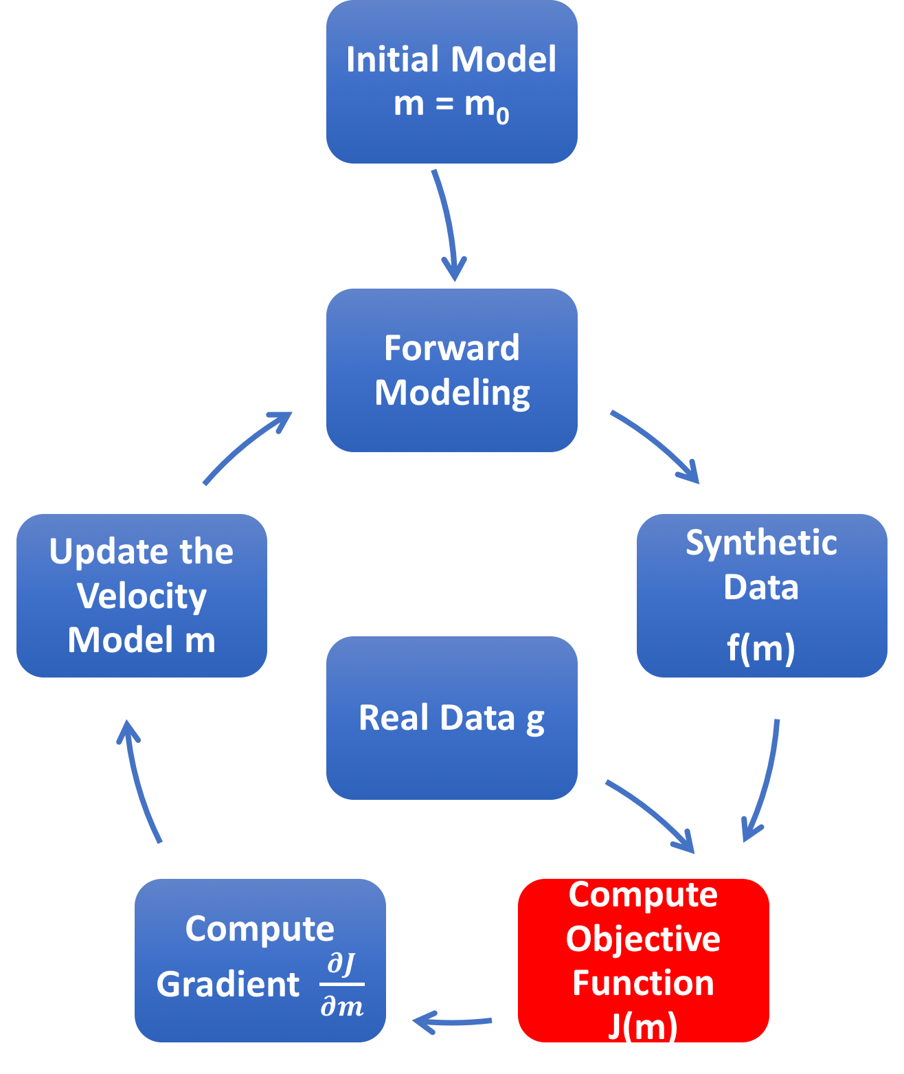
In Figure 3, we highlight the major components of the FWI workflow in each iteration. Starting with an initial velocity parameter, one forward solve gives the synthetic data $f=Ru$. Here, $R$ is an extraction operator that outputs the wavefield $u(\mathbf{x},t)$ on the boundary $\partial\Omega$. $u(\mathbf{x},t)$ is the solution to the following wave equation on spatial domain $\Omega$, from time $0$ to $T_{\text{max}}$:

$$\left\{\begin{array}[]{rl}&m(\mathbf{x})\frac{\partial^{2}u(\mathbf{x},t)}{\partial t^{2}}-\mathop{}\!\mathbin{\bigtriangleup}u(\mathbf{x},t)=s(\mathbf{x},t),\\ &u(\mathbf{x},0)=0,\ \frac{\partial u}{\partial t}(\mathbf{x},0)=0\ \text{on}\ \Omega,\\ &\nabla u\cdot\mathbf{n}=0\ \text{on}\ \partial\Omega.\\ \end{array}\right.$$ (5)

The model parameter is $m(\mathbf{x})=\frac{1}{v(\mathbf{x})^{2}}$ where $v(\mathbf{x})$ is the wave velocity and $s(\mathbf{x},t)$ is the known source term. It is a linear PDE but a nonlinear map from the $m(\mathbf{x})$ to $u(\mathbf{x},t)$. Wave simulation is the most resource-intensive part of the workflow due to the size of the discretized problem in geophysical applications. For realistic applications with hundreds of different wave sources, wave simulations are also done as an embarrassingly parallel task on supercomputers. The difference between the synthetic data $f(m)$ and the real data $g$ is calculated by an objective function $J(m)$. The conventional choice is the least-squares norm ($L^{2}$), as we discussed that suffers from cycle skipping and sensitivity to noise [59]:

$$J_{L^{2}}(m)=\frac{1}{2}\sum_{i_{s}}\int\limits_{\partial\Omega}\int\limits_{0}^{T_{\text{max}}}\left|f_{i_{s}}(\mathbf{x},t;m)-g_{i_{s}}(\mathbf{x},t)\right|^{2}dtd\mathbf{x}.$$

In practice, the objective function is a summation over multiple sources where $i_{s}$ is the index representing the wavefield or data generated by different source term $s(\mathbf{x},t)$ in (5). The summation over the source helps broaden the bandwidth of the observed data, capture waves from various illumination angles, and reduce the effects of noise.

The adjoint-state method is used here to compute the FWI gradient of the objective function; see detailed derivations in [11, 7, 42]. For large-scale PDE-constrained optimizations, the adjoint-state method is a common practice to efficiently compute the gradient of a function or an operator numerically [6]. It has broad applications in general inverse problems beyond seismic imaging [8, 61, 32].

Based on the adjoint-state method [42], one only needs to solve two wave equations numerically to compute the Fréchet derivative or gradient with respect to model parameters in FWI. The first one is the forward propagation (5). The second one is the following adjoint equation on the domain $\Omega$ from time $T_{\text{max}}$ to $0$:

$$\left\{\begin{array}[]{rl}&m\frac{\partial^{2}w(\mathbf{x},t)}{\partial t^{2}}-\mathop{}\!\mathbin{\bigtriangleup}w(\mathbf{x},t)=-R^{*}\frac{\delta J}{\delta f},\\ &w(\mathbf{x},T_{\text{max}})=0,\ \frac{\partial w}{\partial t}(\mathbf{x},T_{\text{max}})=0\ \text{on}\ \Omega,\\ &\nabla w\cdot\mathbf{n}=0\ \text{on}\ \partial\Omega.\\ \end{array}\right.$$ (6)

The adjoint equation above requires zero final condition at time $T_{\text{max}}$. Thus, (6) is often referred to as backpropagation in geophysics. Solving the adjoint equation is also practically done in parallel. Once we have the forward wavefield $u$ and adjoint wavefield $w$, the gradient is calculated as follows

$$~{}\frac{\delta J}{\delta m}=-\sum_{i_{s}}\int_{0}^{T_{\text{max}}}\frac{\partial^{2}u_{i_{s}}(\mathbf{x},t)}{\partial t^{2}}w_{i_{s}}(\mathbf{x},t)dt.$$ (7)

We remark that a modification of the misfit function only impacts the source term of the adjoint wave equation (6) [36].

Using the gradient formula (7), the velocity parameter is updated by an optimization method, as the last step in Figure 3 before entering the next iteration. In this paper, we use L-BFGS with the backtracking line search following the Wolfe conditions [29]. The step size is required to both give a sufficient decrease in the objective function and satisfy the curvature condition [64].

In [66], we proposed a trace-by-trace objective function based on $W_{2}$. A trace is the time history measured at one receiver. The entire dataset consists of the time history of all the receivers. For example, with $\mathbf{x}$ fixed, $f(\mathbf{x},t)$ is a trace. The corresponding misfit function is

$$J_{W_{2}}(m)=\frac{1}{2}\sum_{i_{s}}\int\limits_{\partial\Omega}W_{2}^{2}(f_{i_{s}}(\mathbf{x},t;m),g_{i_{s}}(\mathbf{x},t))d\mathbf{x},$$ (8)

Mathematically it is $W_{2}$ metric in the time domain and $L^{2}$ norm in the spatial domain. In Section 2.2, we will define the $W_{2}$ metric formally.

2.2 Optimal Transport

The optimal mass transport problem seeks the most efficient way of transforming one distribution of mass to the other, relative to a given cost function. It was first brought up by Monge in 1781 [38] and later expanded by Kantorovich [23]. Optimal transport-related techniques are nonlinear as they explore both the signal amplitude and the phases. The significant contributions of the mathematical analysis of optimal transport problem since the 1990s  [57] together with current advancements in numerical methods [39], have driven the recent development of numerous applications based on optimal transport [25].

Given two probability densities $f=d\mu$ and $g=d\nu$, we are interested in the measure-preserving map $T$ such that $f=g\circ T$.

Definition 2.1 (Measure-preserving map).

A transport map $T:X\rightarrow Y$ is measure-preserving if for any measurable set $B\in Y$,

$$~{}\mu(T^{-1}(B))=\nu(B).$$

If this condition is satisfied, $\nu$ is said to be the push-forward of $\mu$ by $T$, and we write $\nu=T_{\#}\mu$.

If the optimal transport map $T(x)$ is sufficiently smooth and $\det(\nabla T(x))\neq 0$, Definition 2.1 naturally leads to the requirement

$$f(x)=g(T(x))\det(\nabla T(x)).$$ (9)

The transport cost function $c(x,y)$ maps pairs $(x,y)\in X\times Y$ to $\mathbb{R}\cup\{+\infty\}$, which denotes the cost of transporting one unit mass from location $x$ to $y$. The most common choices of $c(x,y)$ include $|x-y|$ and $|x-y|^{2}$, which denote the Euclidean norms for vectors $x$ and $y$ hereafter. While there are many maps $T$ that can perform the relocation, we are interested in finding the optimal map that minimizes the total cost. If $c(x,y)=|x-y|^{p}$ for $p\geq 1$, the optimal transport cost becomes the class of Wasserstein metric:

Definition 2.2 (The Wasserstein metric).

We denote by $\mathscr{P}_{p}(X)$ the set of probability measures with finite moments of order $p$. For all $p\in[1,\infty)$,

$$W_{p}(\mu,\nu)=\left(\inf_{T_{\mu,\nu}\in\mathcal{M}}\int_{\mathbb{R}^{n}}\left|x-T_{\mu,\nu}(x)\right|^{p}d\mu(x)\right)^{\frac{1}{p}},\quad\mu,\nu\in\mathscr{P}_{p}(X).$$ (10)

$T_{\mu,\nu}$ is the measure-preserving map between $\mu$ and $\nu$, or equivalently, $(T_{\mu,\nu})_{\#}\mu=\nu$. $\mathcal{M}$ is the set of all such maps that rearrange the distribution $\mu$ into $\nu$.

Equation (10) is based on the Monge’s problem for which the optimal map does not always exist since “mass splitting” is not allowed. For example, consider $\mu=\delta_{1}$ and $\nu=\frac{1}{2}\delta_{0}+\frac{1}{2}\delta_{2}$, where $\delta_{x}$ is the Dirac measure. The only rearrangement from $\mu$ to $\nu$ is not technically a map (function). Kantorovich relaxed the constraints [23] and proposed the following alternative formulation (11). Instead of searching for a function $T$, the transference plan $\pi$ is considered. The plan is a measure supported on the product space $X\times Y$ where $\pi(x,y_{1})$ and $\pi(x,y_{2})$ are well-defined for $y_{1}\neq y_{2}$. The optimal transport problem under the Kantorovich formulation becomes a linear problem in terms of the plan $\pi$:

$$~{}\inf_{\pi}I[\pi]=\bigg{\{}\int_{X\times Y}c(x,y)d\pi\ |\ \pi\geq 0\ \text{and}\ \pi\in\Gamma(\mu,\nu)\bigg{\}},$$ (11)

where $\Gamma(\mu,\nu)=\{\pi\in\mathcal{P}(X\times Y)\ |\ (P_{X})_{\#}\pi=\mu,(P_{Y})_{\#}\pi=\nu\}$. Here $(P_{X})$ and $(P_{Y})$ denote the two projections, and $(P_{X})_{\#}\pi$ and $(P_{Y})_{\#}\pi$ are two measures obtained by pushing forward $\pi$ with these two projections.

One special property of optimal transport is the so-called c-cyclical monotonicity. It offers a powerful tool to characterize the general geometrical structure of the optimal transport plan from the Kantorovich formulation. It has been proved that optimal plans for any cost function have c-cyclically monotone support [58]. In addition, the concept can be used to formulate a sufficient condition of the optimal transport plan [58, 4, 24] under certain mild assumptions [1]. Later, we will use this property to prove Theorem 3.1, one of the key results in the paper.

Definition 2.3 (Cyclical monotonicity).

We say that a set $\xi\subseteq X\times Y$ is c-cyclically monotone if for any $m\in\mathbb{N}^{+}$, $(x_{i},y_{i})\in\xi$, $1\leq i\leq m$, implies

$$\sum_{i=1}^{m}c(x_{i},y_{i})\leq\sum_{i=1}^{m}c(x_{i},y_{i-1}),\ (x_{0},y_{0})\equiv(x_{m},y_{m}).$$

We focus on the quadratic cost ($p=2$) and the quadratic Wasserstein distance ($W_{2}$). We also assume that $\mu$ does not give mass to small sets [4], which is a necessary condition to guarantee the existence and uniqueness of the optimal map under the quadratic cost for Monge’s problem. This requirement is natural for seismic signals. Brenier [4] also proved that the optimal map coincides with the optimal plan in the sense that $\pi=(Id\times T)_{\#}\mu$ if Monge’s problem has a solution. Thus, one can extend the notion of cyclical monotonicity to optimal maps.

The $W_{2}$ distance is related to the Sobolev norm $\dot{H}^{-1}$ [40] and has been proved to be insensitive to mean-zero noise [13, 15]. If both $f=d\mu$ and $g=d\nu$ are bounded from below and above by constants $c_{1}$ and $c_{2}$, the following non-asymptotic equivalence holds,

$$\frac{1}{c_{2}}\|f-g\|_{\dot{H}^{-1}}\leq W_{2}(\mu,\nu)\leq\frac{1}{c_{1}}\|f-g\|_{\dot{H}^{-1}},$$ (12)

where $||f||_{\dot{H}^{-1}}=\big{\|}|\xi|^{-1}\hat{f}(\xi)\big{\|}_{L^{2}}$, $\hat{f}$ is the Fourier transform of $f$, and $\xi$ represents the frequency. If $d\zeta$ is an infinitesimal perturbation that has zero total mass [57],

$$~{}W_{2}(\mu,\mu+d\zeta)=\|d\zeta\|_{\dot{H}_{(d\mu)}^{-1}}+o(d\zeta),$$ (13)

which shows the asymptotic connections. Here, $\dot{H}_{(d\mu)}^{-1}$ is the $\dot{H}^{-1}$ norm weighted by measure $\mu$.

The $1/|\xi|$ weighting suppresses higher frequencies, as seen from the definition of the $\dot{H}^{-1}$ norm. It is also referred to as the smoothing property of the negative Sobolev norms. The asymptotic and non-asymptotic connections in (12) and (13) partially explain the smoothing properties of the $W_{2}$ metric, which applies to any data dimension [15]. It is also a natural result of the optimal transport problem formulation. On the other hand, the $L^{2}$ norm is known to be sensitive to noise [60]. The noise insensitivity of the Wasserstein metric has been used in various applications [27, 45].

Theorem 2.4 ($W_{2}$ insensitivity to noise [13]).

Consider probability density function $f=g+\delta$, where $\delta$ is mean-zero noise (random variable with zero mean) with variance $\eta$, piecewise constant on $N$ intervals (numerical discretization). Then

$$||f-g||_{2}^{2}=\mathcal{O}(\eta),\quad W_{2}^{2}(f,g)=\mathcal{O}\left(\frac{\eta}{N}\right).$$

Remark 2.5.

Theorem 2.4 holds for general (signed) signals of zero mean if the data is normalized by the linear scaling (2).

3 Full-Waveform Inversion with the Wasserstein Metric

A significant source of difficulty in seismic inversion is the high degree of nonlinearity and nonconvexity. FWI is typically performed with the $L^{2}$ norm as the objective function using local optimization algorithms in which the subsurface model is described by using a large number of unknowns, and the number of model parameters is determined a priori [54]. It is relatively inexpensive to update the model through local optimization algorithms, but the convergence highly depends on the choice of a starting model. Mathematically, it is related to the highly nonconvex nature of the PDE-constrained optimization problem and results in finding only local minima.

The current challenges of FWI motivate us to modify the objective function in the general framework in Figure 3 by replacing the traditional $L^{2}$ norm with a new metric of better convexity and stability for seismic inverse problems. Engquist and Froese [12] first proposed to use the Wasserstein distance as an alternative misfit function measuring the difference between synthetic data $f$ and observed data $g$. This new objective function has several properties advantageous for seismic inversion. In particular, the convexity of the objective function with respect to the data translation is a crucial property. Large-scale perturbations of the velocity parameter mainly change the phases of the time-domain signals [22, 60, 13]. The convexity regarding the data shift is the key to avoid the so-called cycle-skipping issues, which is one of the main challenges of FWI. Results regarding the convexity are given in Theorem 3.1 below.

Seismic signals are in both the time and the spatial domain. One can solve a 2D or 3D optimal transport problem to compute the Wasserstein distance [36, 37], or use the trace-by-trace approach (8), which utilizes the explicit solution to the 1D optimal transport problem [57]. It is fast and accurate to compute the Wasserstein distance between 1D signals, so the trace-by-trace approach is cost-effective for implementation. Nevertheless, benefits have been observed regarding the lateral coherency of the data by solving a 2D or 3D optimal transport problem to compute the $W_{2}$ metric [43, 33]. Both approaches have been appreciated by the industry [62, 47]. One can refer to [66, 37] for more discussions.

The translation and dilation in the wavefields are direct effects of variations in the velocity $v$, as can be seen from the D’Alembert’s formula that solves the 1D wave equation [13]. In particular, we will reformulate the theorems in [13] as a joint convexity of $W_{2}$ with respect to both signal translation and dilation and prove it in a more general setting. In practice, the perturbation of model parameters will cause both signal translation and dilation simultaneously, and the convexity with respect to both changes is an ideal property for gradient-based optimization.

Since seismic signals are partial measurements of the boundary value in (5), they are compactly supported in $\mathbb{R}^{d}$ and bounded from above. It is therefore natural to assume

$$\int_{\mathbb{R}^{d}}\int_{\mathbb{R}^{d}}|x-y|^{2}f(x)g(y)dxdy<+\infty.$$ (14)

Normalization is a very important step in seismic inversion that turns oscillatory seismic signals into probability measures. It is one prerequisite of optimal transport [46, 35, 17, 66]. In this section, we regard the normalized synthetic data and observed data as probability densities $f=d\mu$ and $g=d\nu$ compactly supported on convex domains $X,Y\subseteq\mathbb{R}^{d}$, respectively.

Next, we will improve our result in [13] with a stronger convexity proof in the following Theorem 3.1, which states a joint convexity in multiple variables with respect to both translation and dilation changes in the data. Assume that $s_{k}\in\mathbb{R},\ k=1,\dots,d$ is a set of translation parameters and $\{e_{k}\}_{k=1}^{d}$ is the standard basis of the Euclidean space $\mathbb{R}^{d}$. $A=\text{diag}(1/\lambda_{1},\dots,1/\lambda_{d})$ is a dilation matrix where $\lambda_{k}\in\mathbb{R}^{+},k=1,\dots,d$. We define $f_{\Theta}$ as jointly the translation and dilation transformation of function $g$ such that

$$f_{\Theta}(x)=\det(A)g(A(x-\sum_{k=1}^{d}s_{k}e_{k})).$$ (15)

We will prove the convexity in terms of the multivariable

$$\Theta=\{s_{1},\dots,s_{d},\lambda_{1},\dots,\lambda_{d}\}\in\mathbb{R}^{2d}.$$

Theorem 3.1 (Convexity of $W_{2}$ in translation and dilation).

Let $g=d\nu$ be a probability density function with finite second moment and $f_{\Theta}$ is defined by (15). If, in addition, $g$ is compactly supported on convex domain $Y\subseteq\mathbb{R}^{d}$, the optimal transport map between $f_{\Theta}(x)$ and $g(y)$ is $y=T_{\Theta}(x)$ where $\langle T_{\Theta}(x),e_{k}\rangle=\frac{1}{\lambda_{k}}(\langle x,e_{k}\rangle-s_{k}),k=1,\dots,d$. Moreover, $I(\Theta)=W_{2}^{2}(f_{\Theta}(x),g)$ is a strictly convex function of the multivariable $\Theta$.

Proof of Theorem 3.1.

First, we will justify that $y=T_{\Theta}(x)$ is a measure-preserving map according to Definition 2.1. It is sufficient to check that $T_{\Theta}$ satisfies Equation (9):

$$f_{\Theta}(x)=\det(A)g(T_{\Theta}(x))=\det(\nabla T_{\Theta}(x))g(T_{\Theta}(x)).$$

Since $f_{\Theta}$ and $g$ have finite second moment by assumption, (14) holds. Next, we will show that the new joint measure $\pi_{\Theta}=(Id\times T_{\Theta})\#\mu_{\Theta}$ is cyclically monotone. This is based on two lemmas from [57, p80] and the fundamental theorem of optimal transport in [1, p10] on the equivalence of optimality and cyclical monotonicity under the assumption of  (14).

For $c(x,y)=|x-y|^{2}$, the cyclical monotonicity in Definition 2.3 is equivalent to

$$\sum_{i=1}^{m}x_{i}\cdot(T(x_{i})-T(x_{i-1}))\geq 0,$$

for any given set of $\{x_{i}\}_{i=1}^{m}\subset X$. For $T_{\Theta}(x)$, we have

$$\sum_{i=1}^{m}x_{i}\cdot(T_{\Theta}(x_{i})-T_{\Theta}(x_{i-1})) =\sum_{i=1}^{m}\sum_{k=1}^{d}\langle x_{i},e_{k}\rangle\cdot(\langle T_{\Theta}(x_{i}),e_{k}\rangle-\langle T_{\Theta}(x_{i-1}),e_{k}\rangle)$$

$$=\sum_{i=1}^{m}\sum_{k=1}^{d}\frac{1}{\lambda_{k}}\langle x_{i},e_{k}\rangle\cdot(\langle x_{i},e_{k}\rangle-\langle x_{i-1},e_{k}\rangle)$$

$$=\frac{1}{2}\sum_{k=1}^{d}\frac{1}{\lambda_{k}}\sum_{i=1}^{m}|\langle x_{i},e_{k}\rangle-\langle x_{i-1},e_{k}\rangle|^{2}\geq 0,$$ (16)

which indicates that the support of the transport plan $\pi_{\Theta}=(Id\times T_{\Theta})\#\mu_{\Theta}$ is cyclically monotone. By the uniqueness of monotone measure-preserving optimal maps between two distributions [31], we assert that $T_{\Theta}(x)$ is the optimal map between $f_{\Theta}$ and $g$. The squared $W_{2}$ distance between $f_{\Theta}$ and $g$ is

$$I(\Theta)=W_{2}^{2}(f_{\Theta},g) =\int_{X}|x-T_{\Theta}(x)|^{2}f_{\Theta}(x)dx$$

$$=\int_{Y}\sum_{k=1}^{d}|(\lambda_{k}-1)\langle y,e_{k}\rangle+s_{k}|^{2}d\nu$$

$$=\sum_{k=1}^{d}a_{k}(\lambda_{k}-1)^{2}+2\sum_{k=1}^{d}b_{k}s_{k}(\lambda_{k}-1)+\sum_{k=1}^{d}s_{k}^{2},$$ (17)

where $a_{k}=\int_{Y}|\langle y,e_{k}\rangle|^{2}d\nu$ and $b_{k}=\int_{Y}\langle y,e_{k}\rangle d\nu$.

$I(\Theta)$ is a quadratic function whose Hessian matrix $H(\Theta)$ is

$$\begin{pmatrix}I_{s_{1}s_{1}}&\dots&I_{s_{1}s_{d}}&I_{s_{1}\lambda_{1}}&\dots&I_{s_{1}\lambda_{d}}\\ \vdots&\ddots&\vdots&\vdots&\ddots&\vdots\\ I_{s_{d}s_{1}}&\dots&I_{s_{d}s_{d}}&I_{s_{d}\lambda_{1}}&\dots&I_{s_{d}\lambda_{d}}\\ I_{\lambda_{1}s_{1}}&\dots&I_{\lambda_{1}s_{d}}&I_{\lambda_{1}\lambda_{1}}&\dots&I_{\lambda_{1}\lambda_{d}}\\ \vdots&\ddots&\vdots&\vdots&\ddots&\vdots\\ I_{\lambda_{d}s_{1}}&\dots&I_{\lambda_{d}s_{d}}&I_{\lambda_{d}\lambda_{1}}&\dots&I_{\lambda_{d}\lambda_{d}}\\ \end{pmatrix}=2\,\begin{pmatrix}1&\dots&0&b_{1}&\dots&0\\ \vdots&\ddots&\vdots&\vdots&\ddots&\vdots\\ 0&\dots&1&0&\dots&b_{d}\\ b_{1}&\dots&0&a_{1}&\dots&0\\ \vdots&\ddots&\vdots&\vdots&\ddots&\vdots\\ 0&\dots&b_{d}&0&\dots&a_{d}\\ \end{pmatrix}.$$

$H(\Theta)$ is a symmetric matrix with eigenvalues:

$$a_{k}+1\pm\sqrt{a_{k}^{2}-2a_{k}+4b_{k}^{2}+1},\ k=1,\dots,d.$$

Since $a_{k}=\int_{Y}|\langle y,e_{k}\rangle|^{2}d\nu\geq 0$ by definition, and

$$\quad\left(a_{k}+1\right)^{2}-\left(\sqrt{a_{k}^{2}-2a_{k}+4b_{k}^{2}+1}\right)^{2}$$

$$=4\left(\int_{Y}|\langle y,e_{k}\rangle|^{2}d\nu\int_{Y}1^{2}d\nu-\left(\int_{Y}\langle y,e_{k}\rangle d\nu\right)^{2}\right)$$

$$\geq 0\quad\text{by Cauchy-Schwarz inequality},~{}$$ (18)

all the eigenvalues of $H(\Theta)$ are nonnegative. Given any $k=1,\dots,d$, the equality in (18) holds if and only if $l(y)=|\langle y,e_{k}\rangle|^{2}$ is a constant function, $\forall y\in Y$, which contradicts the fact that $Y$ is a convex domain. Therefore, the Hessian matrix of $I(\Theta)$ is symmetric positive definite, which completes our proof that $W_{2}^{2}(f_{\Theta},g)$ is a strictly convex function with respect to $\Theta=\{s_{1},\dots,s_{d},\lambda_{1},\dots,\lambda_{d}\}$, the combination of translation and dilation variables. ∎

Figure 4: $W^{2}_{2}(f_{[\mu,\sigma]},g)$ where $f_{[\mu,\sigma]}$ and $g$ are probability density functions of normal distribution $\mathcal{N}(\mu,\sigma^{2})$ and $\mathcal{N}(0,1)$.

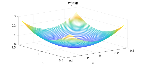
In Figure 4, we illustrate the joint convexity of the squared $W_{2}$ distance with respect to both translation and dilation by comparing density functions of normal distributions. We set $f_{[\mu,\sigma]}$ as the density function of the 1D normal distribution $\mathcal{N}(\mu,\sigma^{2})$. The reference function $g$ is the density of $\mathcal{N}(0,1)$. Figure 4 is the optimization landscape of $W^{2}_{2}(f_{[\mu,\sigma]},g)$ as a multivariable function. It is globally convex with respect to both translation $\mu$ and dilation $\sigma$.

Note that Theorem 3.1 applies when $f$ and $g$ are probability density functions, which is not the case for seismic data. We will discuss more on this topic in Section 4. Let us consider that we can transform the data into density functions and compute the $W_{2}$ distance. The convexity of the “normalized” $W_{2}$ with respect to translation and dilation depends on the choice of normalization function. We will prove that the softplus scaling (4) still keeps the good convexity when the hyperparameter $b$ in (4) is large.

4 Data Normalization

We discuss the intrinsic convexity of the Wasserstein distance in Section 3, but the fact that functions should be restricted to probability distributions is the primary constraint of applying optimal transport to general signals, in particular, oscillatory seismic waves. So far, mathematical extensions of the optimal transport theory to signed measures are quite limited [30, 2]. Different strategies have been proposed in the literature to tackle this issue numerically.

The dual formulation of the 1-Wasserstein distance ($W_{1}$) coincides in expression with the so-called Kantorovich Rubinstein (KR) norm while the latter is well-defined for all functions. Using the KR norm as an alternative to $W_{1}$ is a feasible approach in seismic inversion [36, 37]. Another interesting strategy is to map the discrete signed signals into a graph space and then compare the Wasserstein distance between the obtained point clouds [50, 55, 35, 34]. One can also choose to penalize the matching filter between datasets to be an identity based on the Wasserstein metric instead of working with the data itself [51, 52]. Here, we focus on a different approach: to transform the data into probability density functions using a nonlinear scaling function before the comparison.

Since properties of the Wasserstein distance are deeply rooted in the theory of optimal transport, which studies probability measures, all the strategies above have advantages as well as limitations. It is efficient to compute the KR norm for 2D and 3D data, but the norm does not preserve the convexity regarding data shifts. The graph-based idea may preserve the convexity if the displacements along with the amplitude and the phase are well-balanced, but inevitably increases the dimensionality of the optimal transport problem. Compared to these strategies, the approach we present here is remarkably efficient as it does not increase the dimensionality of the data such that it uses the closed-form solution to the 1D optimal transport problem. The benefits in terms of computational costs are significant for practical large-scale applications.

We have discussed normalization before in [46, 17], but not until here are any rigorous results given. In [12], the signals were separated into positive and negative parts $f^{+}=\max\{f,0\}$, $f^{-}=\max\{-f,0\}$ and scaled by the total sum. However, the approach cannot be combined with the adjoint-state method [42], while the latter is essential to solve large-scale problems. This separation scaling introduces discontinuities in derivatives from $f^{+}$ or $f^{-}$, and the discontinuous Fréchet derivative of the objective function with respect to $f$ cannot be obtained. The squaring $f^{2}$ or the absolute-value scaling $\left|f\right|$ are not ideal either since they are not one-to-one maps, and consequently lead to nonuniqueness and potentially more local minima for the optimization problem (1). One can refer to [17] for more discussions.

Later, the linear scaling (2) [66] and the exponential-based methods [46], (3) and (4) are observed to be effective in practice. The main issue of data normalization is how to properly transform the data, as one can see from the literature or practice that some scaling methods seem to work better than others. This section focuses on presenting several useful scaling methods and explaining their corresponding impacts on the $W_{2}$ misfit function. We aim to offer better understandings of the role that the normalization function plays in inversion. First, we generalize the class of effective normalization functions that satisfy Assumption 4.1.

Assumption 4.1.

Given a scaling function $\sigma:\mathbb{R}\rightarrow\mathbb{R}^{+}$, we define the normalization operator $P_{\sigma}$ on function $f:\Pi\rightarrow\mathbb{R}$ as follows: for $x\in\Pi_{1},\ t\in\Pi_{2}$ where $\Pi=\Pi_{1}\times\Pi_{2}$,

$$(P_{\sigma}f)(x,t)=\dfrac{\sigma(y(x,t))+c}{S_{\sigma}(x)},\quad S_{\sigma}(x)=\int_{\Pi_{2}}\left(\sigma(f(x,\tau))+c\right)d\tau,\quad c\geq 0.$$ (19)

The scaling function $\sigma$ satisfies the following assumption

1. $\sigma$ is one-to-one;

2. $\sigma:\mathbb{R}\rightarrow\mathbb{R}^{+}$ is a $C^{\infty}$ function.

Functions that satisfy Assumption 4.1 include the linear scaling $\sigma_{l}(x;b)$, the exponential scaling $\sigma_{e}(x;b)$ and the softplus function $\sigma_{s}(x;b)$, where $b$ is a hyperparameter. We use the definition “hyperparameter” to distinguish it from the velocity parameter that are determined in the inversion process.

$$\sigma_{l}(x;b)=x+b,\qquad\sigma_{e}(x;b)=\exp(bx),\qquad\sigma_{s}(x;b)=\log\left(\exp(bx)+1\right).$$

Equivalent definitions are in Equation (2), (3) and (4).

In the rest of Section 4, we prove several properties for the class of normalization operators that satisfy Assumption 4.1 and discuss their roles in improving optimal transport-based FWI. Since the normalization (19) is performed on a domain $\Pi_{2}$, and the properties apply for any $x\in\Pi_{1}$, we will assume $f$ and $g$ are functions that are defined on the domain $\Pi_{2}$ (instead of $\Pi$) for the rest of the section. As mentioned in Section 2.1, we consider the trace-by-trace approach (1D optimal transport) for seismic inversion. Hence, $\Pi_{2}\subseteq\mathbb{R}$, but all the properties in this section hold for $\Pi_{2}\subseteq\mathbb{R}^{d},d\geq 2$ as well.

4.1 A Metric for Signed Measures

Let $\mathcal{P}_{s}({\Pi_{2}})$ be the set of finite signed measures that are compactly supported on domain ${\Pi_{2}}\subseteq\mathbb{R}^{d}$. Consider $f=d\mu$ and $g=d\nu$ where $\mu,\nu\in\mathcal{P}_{s}({\Pi_{2}})$. We denote $\tilde{f}=P_{\sigma}(f)$ and $\tilde{g}=P_{\sigma}(g)$ as normalized probability densities, where $P_{\sigma}$ is any scaling operator that satisfies Assumption 4.1. We shall use $W_{2}(\tilde{f},\tilde{g})$ as the objective function measuring the misfit between original seismic signals $f$ and $g$. It can also be viewed as a new loss function $W_{\sigma}(f,g)=W_{2}(\tilde{f},\tilde{g})$ which defines a metric between $f$ and $g$.

Theorem 4.2 (Metric for signed measures).

Given $P_{\sigma}$ that satisfies Assumption 4.1, $W_{\sigma}$ defines a metric on $\mathcal{P}_{s}({\Pi_{2}})$.

Proof.

Since $W_{2}$ is a metric on probability measures with finite second moment, $W_{\sigma}$ is symmetric, nonnegative and finite on $\mathcal{P}_{s}({\Pi_{2}})$. Also, we have that

$$W_{\sigma}(f,f)=W_{2}(P_{\sigma}(f),P_{\sigma}(f))=0.$$

If $W_{\sigma}(f,g)=0$, then the following holds:

$$P_{\sigma}(f)=\frac{\sigma(f)+c}{\int_{\Pi_{2}}\sigma(f(\tau))d\tau+c|{\Pi_{2}}|}=\frac{\sigma(g)+c}{\int_{\Pi_{2}}\sigma(g(\tau))d\tau+c|{\Pi_{2}}|}=P_{\sigma}(g).$$

Since $f$ and $g$ are both compactly supported on ${\Pi_{2}}$, $\exists x^{*}\in{\Pi_{2}}$ such that $f(x^{*})=g(x^{*})=0$. Together with $\tilde{f}(x^{*})=\tilde{g}(x^{*})$, we have

$$\int_{\Pi_{2}}\sigma(f(\tau))d\tau=\frac{\sigma(f(x^{*}))+c}{(P_{\sigma}f)(x^{*})}-c|{\Pi_{2}}|=\frac{\sigma(g(x^{*}))+c}{(P_{\sigma}g)(x^{*})}-c|{\Pi_{2}}|=\int_{\Pi_{2}}\sigma(g(\tau))d\tau.$$

Together with (4.1) and the fact that $\sigma$ is one-to-one, we have $f=g$ on ${\Pi_{2}}$.

All that remains to check is the triangle inequality. Consider $h=d\rho$ where $\rho\in\mathcal{P}_{s}({\Pi_{2}})$.

$$W_{\sigma}(f,g)+W_{\sigma}(g,h) =W_{2}(\tilde{f},\tilde{g})+W_{2}(\tilde{g},\tilde{h})$$

$$\leq W_{2}(\tilde{f},\tilde{h})=W_{\sigma}(f,h).$$

∎

Remark 4.3 (Variance and invariance under mass subtraction).

One can extend the optimal mass transportation problem between nonnegative measures whose mass is not normalized to unity [57]. Unlike the 1-Wasserstein distance ($W_{1}$) which corresponds to the case of $p=1$ in (10), $W_{2}(f,g)$ is not invariant under mass subtraction. This property can easily be extended to a set of functions $\{\bar{h}\in L^{2}({\Pi_{2}}):f+\bar{h}\geq 0,g+\bar{h}\geq 0\}$ since generally

$$W_{2}(f+\bar{h},g+\bar{h})\neq W_{2}(f,g),$$

while the $L^{2}$ norm and the $W_{1}$ distance remain unchanged:

$$||(f+\bar{h})-(g+\bar{h})||_{L^{2}}=||f-g||_{L^{2}},$$

$$W_{1}(f+\bar{h},g+\bar{h})=W_{1}(f,g).$$

$W_{2}$ has the unique feature of variance under mass subtraction/addition. Later, we will see that this feature gives us the Huber-type property (Theorem 4.6) and regularization effects (Theorem 4.8) by adding a positive constant $c$ to the signals.

4.2 Hyperparameter $b$: Effects on Convexity

We list three specific scaling functions that satisfy Assumption 4.1, i.e., (2), (3) and (4). In particular, the exponential scaling and the softplus function are defined by the hyperparameter $b$, which controls the convexity of the normalized Wasserstein distance. Without loss of generality, we set $c=0$ in (19).

(a) Linear scaling

(b) Exponential (small $b$)

(c) Exponential (large $b$)

(d) Softplus (small $b$)

(e) Softplus (large $b$)

Figure 5: Optimization landscape of the $W_{2}$ metric between Ricker wavelets $f(x)$ and $f(x-s)$, generated by (a) the linear, (b)(c) the exponential with small and large $b$ and (d)(e) the softplus scaling with small and large $b$.

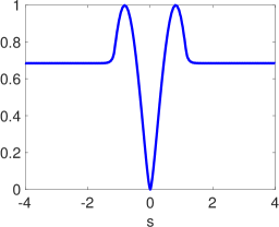
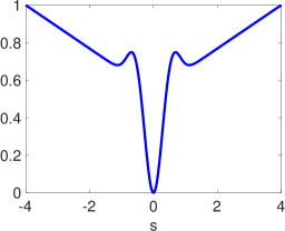
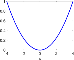
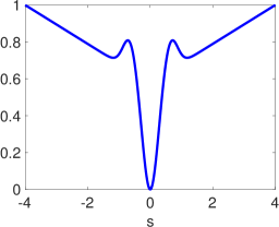
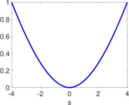
We compare the optimization landscape of the normalized $W_{2}$ metric between function $f(x)$ and its shift $f(x-s)$. The linear scaling affects the convexity of $W_{2}$ with respect to translation [17]; see Figure 5a. Figure 5b and 5c are obtained by the exponential scaling. We choose scalar $b$ such that $||bf||_{\ell_{\infty}}\approx 0.5$ in Figure 5b and $||bf||_{\ell_{\infty}}\approx 4$ in Figure 5c. The objective function plot in Figure 5c is more quadratic than the one in Figure 5b, while the latter is nonconvex. The larger the $b$, the more suppressed the negative counterparts of the waveform. Similar patterns are also observed in Figure 5d and 5e for the softplus scaling function. Nevertheless, one should note that an extremely large $b$ is not preferred for the exponential scaling due to the risk of noise amplification and potentially machine overflow. Empirically, $b$ should be chosen properly in the range $0.2\leq||bf||_{\ell_{\infty}}\leq 6$. In this sense, the softplus scaling $\sigma_{s}$ is more stable than the exponential scaling.

We present an extended result based on Theorem 3.1. Here, we consider signed functions $g$ and $f_{\Theta}$ defined by (15), compactly supported on $\Pi_{\mathscr{K}},\forall\Theta\in\mathscr{K}$. Here, $\mathscr{K}$ is a compact subset of $\mathbb{R}^{2d}$ which represents the set of transformation parameters. Under these assumptions, the convexity of the $W_{2}$ metric is preserved when comparing signed functions.

Corollary 4.4 (Convexity of $W_{2}$ with the softplus scaling).

Let $\widetilde{f_{\Theta,b}}$ and $\widetilde{g_{b}}$ be normalized functions of $f_{\Theta}$ and $g$ based on the softplus scaling (4) with hyperparameter $b$. Then, there is $b^{*}\in\mathbb{R}^{+}$ such that $I(\Theta,b)=W^{2}_{2}(\widetilde{f_{\Theta,b}},\widetilde{g_{b}})$ is strictly convex with respect to $\Theta$ if $b>b^{*}$.

Proof.

One key observation is that $I(\Theta,b)$ is a smooth function of multivariable $\Theta$ and the scalar variable $b$. As $b\rightarrow+\infty$,

$$\lim\limits_{b\rightarrow+\infty}\widetilde{f_{\Theta,b}}=\frac{f_{\Theta}^{+}}{\int_{\Pi_{\mathscr{K}}}f_{\Theta}^{+}}\coloneqq\widetilde{f_{\Theta}^{+}}\quad,\lim\limits_{b\rightarrow+\infty}\widetilde{g_{b}}=\frac{g^{+}}{\int_{\Pi_{\mathscr{K}}}g^{+}}\coloneqq\widetilde{g^{+}}.$$

Since $\widetilde{f_{\Theta}^{+}}$ and $\widetilde{g^{+}}$ are nonnegative functions with equal total sum, $\lim\limits_{b\rightarrow+\infty}I(\Theta,b)=W_{2}^{2}(\widetilde{f_{\Theta}^{+}},\widetilde{g^{+}})$ is strictly convex in $\Theta$ by Theorem 3.1. The Hessian of $W_{2}^{2}(\widetilde{f_{\Theta}^{+}},\widetilde{g^{+}})$ in $\Theta$, $H^{+}(\Theta)$, is symmetric positive definite, for all $\Theta\in\mathscr{K}$. If we denote the Hessian of $I(\Theta,b)$ with respect to $\Theta$ as $H(\Theta,b)$ which is also a matrix valued smooth function in $\Theta$ and $b$, then $\lim\limits_{b\rightarrow+\infty}H(\Theta,b)=H_{\Theta}^{+}$. Therefore, there is a $b^{*}$ such that when $b>b^{*}$, $H(\Theta,b)$ is symmetric positive definite for all $\Theta\in\mathscr{K}$, which leads to the conclusion of the corollary. ∎

4.3 Hyperparameter $c$: Huber-Type Property

While the choice of $b$ is essential for preserving the ideal convexity of the $W_{2}$ metric with respect to shifts (Theorem 3.1), the other hyperparameter $c\geq 0$ in (19) regularizes the quadratic Wasserstein metric as a “Huber-type” norm, which can be generalized to the entire class of normalization functions that satisfies Assumption 4.1. In statistics, the Huber norm [21] is a loss function used in robust regression, that is less sensitive to outliers in data than the squared error loss. For a vector $\mathbf{\eta}$, the Huber norm of $s\mathbf{\eta}$, $s\geq 0$, is $\mathcal{O}(s^{2})$ for small $s$ and $\mathcal{O}(s)$ once $s$ is larger than a threshold. For optimal transport-based FWI, the Huber property is good for not overemphasizing the mass transport between seismic events that are far apart and physically unrelated as $s^{2}\gg s$ for large $s$. The big-O notation is defined as follows.

Definition 4.5 (Big-O notation).

Let $f$ and $g$ be real-valued functions with domain $\mathbb{R}$. We say $f(x)=\mathcal{O}(g(x))$ if there are positive constants $M$ and $k$, such that $|f(x)|\leq M|g(x)|$ for all $x\geq k$. The values of $M$ and $k$ must be fixed for the function $f$ and must not depend on $x$.

Assuming ${\Pi_{2}}\subseteq\mathbb{R}$, we will next show that the positive constant $c$ in the data normalization operator $P_{\sigma}$, defined in (19), turns the $W_{2}$ metric into a “Huber-type” norm . The threshold for the transition between $\mathcal{O}(s^{2})$ and $\mathcal{O}(s)$ depends on the constant $c$ and the support ${\Pi_{2}}$. The constant $c$ is added after signals become nonnegative, and the choice of $\sigma$ in Assumption 4.1 is independent of the Huber-type property. Without loss of generality, we state the theorem in the context of probability densities to avoid unrelated discussions on making data nonnegative.

Theorem 4.6 (Huber-type property for 1D signal).

Let $f$ and $g$ be probability density functions compactly supported on ${\Pi_{2}}\subseteq\mathbb{R}$ and $g(x)=f(x-s)$ on ${\Pi^{s}_{2}}=\{x\in\mathbb{R}:x-s\in{\Pi_{2}}\}$ and zero otherwise. Consider $\tilde{f}$ and $\tilde{g}$ as new density functions defined by linear normalization (2) for a given $c>0$, then

$$W^{2}_{2}(\tilde{f},\tilde{g})=\begin{cases}\mathcal{O}(|s|^{2}),&\text{if $|s|\leq\frac{1}{c}+|\operatorname{supp}(f)|$},\\ \mathcal{O}(|s|),&\text{otherwise}.\end{cases}$$

Proof.

Without loss of generality, we assume $f$ is compactly supported on an interval $[a_{1},a_{2}]\subseteq{\Pi_{2}}$ and $s\geq 0$. Note that $\tilde{f}$ and $\tilde{g}$ are no longer compactly support on the domain ${\Pi_{2}}$. In one dimension, one can solve the optimal transportation problem explicitly in terms of the cumulative distribution functions

$$F(x)=\int_{0}^{x}f(t)\,dt,\quad G(x)=\int_{0}^{x}g(t)\,dt.$$

It is well known [57, Theorem 2.18] that the optimal transportation cost is

$$W_{2}^{2}(f,g)=\int_{0}^{1}|F^{-1}(t)-G^{-1}(t)|^{2}\,dt.$$ (20)

If additionally the target density $g$ is positive, the optimal map from $f$ to $g$ becomes

$$T(x)=G^{-1}(F(x)).$$ (21)

Based on the 1D explicit formula (20),

$$\begin{split}&W^{2}_{2}(\tilde{f},\tilde{g})=\int_{0}^{1}|\tilde{F}^{-1}(y)-\tilde{G}^{-1}(y)|^{2}dy=\\ &\begin{cases}2\int_{y_{1}}^{y_{3}}|{F}^{-1}(y)-\frac{y}{c_{1}}|^{2}dy+\int_{y_{3}}^{y_{2}}|{F}^{-1}(y)-{F}^{-1}(y-c_{1}s)+s|^{2}dy,&|s|\leq\frac{1}{c}+|a_{2}-a_{1}|,\\ 2\int_{y_{1}}^{y_{2}}|\tilde{F}^{-1}(y)-\frac{y}{c_{1}}|^{2}dy+\int_{y_{2}}^{y_{3}}\frac{1}{c^{2}}dy,&\text{otherwise}.\end{cases}\end{split}$$

Here $F,G,\tilde{F},\tilde{G}$ are cumulative distribution functions of $f,g,\tilde{f},\tilde{g}$ respectively. $|{\Pi_{2}}|$ denotes the Lebesgue measure of the bounded domain ${\Pi_{2}}$, $c_{1}=\frac{c}{1+c|{\Pi_{2}}|}$, $y_{1}=c_{1}a_{1}$, $y_{2}=c_{1}a_{2}+\frac{1}{1+c|{\Pi_{2}}|}$ and $y_{3}=c_{1}a_{1}+c_{1}s$. Since $y_{1}$ and $y_{2}$ are independent of $s$, it is not hard to show that $W^{2}_{2}(\tilde{f},\tilde{g})$ is linear in $s$ if $s>\frac{1}{c}+|a_{2}-a_{1}|$ while $W^{2}_{2}(\tilde{f},\tilde{g})=\mathcal{O}(s^{2})$ if $0\leq s\leq\frac{1}{c}+|a_{2}-a_{1}|$. ∎

Remark 4.7.

For higher dimensions ${\Pi_{2}}\subseteq\mathbb{R}^{d}$, choosing the map $T$ along the shift direction gives $W_{2}^{2}(\tilde{f},\tilde{g})\leq\mathcal{O}(s)$ for large $s$. The optimal map can reduce $W_{2}^{2}(\tilde{f},\tilde{g})$ to $\mathcal{O}(\log(s))$ if $d=2$, which grows more slowly as $s$ increases. We focus on $d=1$ and do not elaborate the details for higher dimensions here since the trace-by-trace approach (8) is mainly used in this paper and also in practice.

Based on the subadditivity of the $W_{2}$ distance under rescaled convolution [57],

$$W_{2}^{2}(\tilde{f},\tilde{g})=W_{2}^{2}(\frac{{f}+c}{1+c|{\Pi_{2}}|},\frac{{g}+c}{1+c|{\Pi_{2}}|})\leq\frac{W_{2}^{2}({f},{g})}{(1+c|{\Pi_{2}}|)^{2}}\leq W_{2}^{2}({f},{g}).$$

The inequality shows that adding a constant $c$ to the data decreases the loss computed by the original objective function and explains the “Huber-type” property.

(a)

(b)

(c)

(d)

Figure 6: (a) The original signal $f$ and $g=f(t-s)$; (b) normalized signals $\tilde{f}$ and $\tilde{g}$ with $c=0$ and (c) with $c=2$ in (19); parameter $b$ is fixed in both (b) and (c). (d) The Huber effect of linear constant $c$ on the loss function $W(\tilde{f},\tilde{g})$ as a function of the shift $s$.

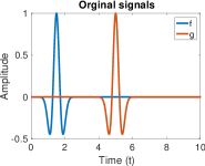
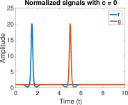
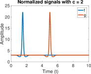
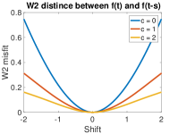
The Huber-type property is also often observed in numerical tests. Consider functions $f$ and $g$ where $f$ is a single Ricker wavelet and $g=f(t-s)$; see Figure 6a. We apply the softplus scaling $\sigma_{s}$ in (4) to obtain probability densities $\tilde{f}$ and $\tilde{g}$. According to Corollary 4.4, with a proper choice of the hyperparameter $b$, the convexity proved in Theorem 3.1 holds. Thus, the Huber-type property proved in Theorem 4.6 still applies. With $b$ fixed, Figure 6d shows the optimization landscape of the objective function with respect to shift $s$ for different choices of $c$. We observe that as $c$ increases, the objective function becomes less quadratic and more linear for the large shift, which conveys the same message as Theorem 4.6. Figure 6b shows the normalized Ricker wavelets for $c=0$ while Figure 6c shows the data with constant $c=2$ applied in (19). The major differences between the original signal and the normalized ones are that we suppress the negative counterparts of the wavelets while stretching the positive peaks. The phases remain unchanged, and the original signal can be recovered since $\sigma_{s}$ is a one-to-one function that satisfies Assumption 4.1.

4.4 The Gradient-Smoothing Property

In this section, we demonstrate another important property, which is to improve the regularity of the optimal map $T$, as a result of adding the constant $c$ in (19).

(a)

(b)

Figure 7: The black arrows represent the optimal map $T$. (a) Function $f$ is compactly supported on $[3.5,6.5]$. Function $g$ is compactly supported on $[0,3]\cup[7,10]$. The optimal map between $f$ and $g$ is discontinuous at $t=5$. (b) Signals $f$ and $g$ after linear normalization. The optimal map $T$ becomes a continuous function by adding the constant $c=0.3$ as stated in Theorem 4.8.

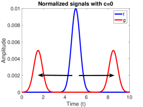
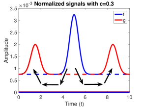
Based on the settings of optimal transport problem, the optimal map is often discontinuous even if $f,g\in C^{\infty}$; see Figure 7a for an example in which the corresponding cumulative distribution functions $F$ and $G$ are monotone but not strictly monotone. However, by adding a positive constant $c$ to the signals, we have improved the smoothness for the optimal map, as seen in Figure 7b. The smoothing property is based on the following Theorem 4.8. Since the positive constant $c$ is applied after the signed functions are normalized to be probability densities in Assumption 4.1, we will hereafter show the improved regularity by applying the linear scaling (2) to the probability densities with a positive constant $c$.

Theorem 4.8 (The smoothing property in the map).

Consider bounded probability density functions $f,g\in C^{k,\alpha}({\Pi_{2}})$ where ${\Pi_{2}}$ is a bounded convex domain in $\mathbb{R}^{d}$ and $0<\alpha<1$. If the normalized signals $\tilde{f}$ and $\tilde{g}$ are obtained by the linear scaling (2) with $c>0$, then the optimal map $T$ between $\tilde{f}$and $\tilde{g}$ is $C^{k+1,\alpha}({\Pi_{2}})$.

Proof.

We first consider the case of $d=1$. By adding a nonzero constant to $f$ and $g$, we guarantee that the cumulative distribution function of $\tilde{f}$ and $\tilde{g}$, i.e., $\tilde{F}$ and $\tilde{G}$, to be strictly monotone and thus invertible in the classical sense. The optimal map $T$ is explicitly determined in (21). Since $f,g\in C^{k,\alpha}$, $\tilde{F},\tilde{G},\tilde{F}^{-1},\tilde{G}^{-1}$ and $T$ are all in $C^{k+1,\alpha}$.

For higher dimensions $d\geq 2$, one can characterize the optimal map by the following Monge-Ampère equation [4]:

$$\det(D^{2}u(x))=\frac{\tilde{f}(x)}{\tilde{g}(\nabla u(x))},\quad x\in{\Pi_{2}}.$$ (22)

Note that $\tilde{f}$ and $\tilde{g}$ are bounded from below by $\frac{c}{1+c|{\Pi_{2}}|}$. Thus, $\frac{\tilde{f}}{\tilde{g}}\in C^{k,\alpha}({\Pi_{2}})$. Since $\Pi_{2}$ is convex, Caffarelli’s regularity theory for optimal transportation applies [5]. Thus, the solution $u$ to (22) is $C^{k+2,\alpha}$ and the optimal transport map $T=\nabla u$ is $C^{k+1,\alpha}$ [4]. ∎

One advantage of adding a constant in the data normalization (19) is to enlarge $\mathcal{M}$, the set of all maps that rearrange the distribution $f$ into $g$. For example, $f$ and $g$ shown in Figure 7a are $C^{\infty}$ functions, but all feasible measure-preserving maps between them are discontinuous. After normalizing $f$ and $g$ by adding a positive constant such that they are strictly positive, smooth rearrangement maps are available, and the optimal one is a $C^{\infty}$ function for the case in Figure 7b.

The regularity of the optimal map is crucial for optimal transport based seismic inversion, particularly for low-wavenumber reconstruction. A smooth optimal map improves the smoothness of the data Fréchet derivative $\frac{\delta J}{\delta f}$ where $J$ is the squared $W_{2}$ metric. We will prove the statement in Corollary 4.9. The term $\frac{\delta J}{\delta f}$ is also the source of the adjoint wave equation (6), which directly determines the frequency content of the adjoint wavefield $w$. We recall that the model gradient $\frac{\delta J}{\delta m}$ is computed as a convolution of the forward and the adjoint wavefields, $u$ and $w$ in (7). Thus, a smoother source term for the adjoint wave equation (6) results in a smoother adjoint wavefield $w$, and therefore a smoother model gradient $\frac{\delta J}{\delta m}$. A smoother gradient can be seen as low-pass filtering of the original gradient and thus focuses on low-wavenumber content for the subsurface model update.

(a)

(b)

Figure 8: (a) The $W_{2}$ data gradient (24) by linear scaling with $c=1$ (blue) and $c=0$ (red); (b) the Fourier transform of the functions in (a).

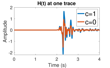
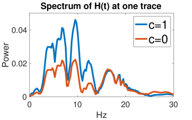
Figure 8 shows a 1D example in which the adjoint source has stronger low-frequency modes after data normalization following (19) with $c>0$ than the one corresponding to the normalization with $c=0$. The following corollary states the general smoothing effect in the gradient by adding a positive constant $c$ in the normalization of data.

Corollary 4.9 (The smoothing effect in the gradient).

Under the same assumptions of Theorem 4.8, the Fréchet derivative of $W_{2}(\tilde{f},\tilde{g})$ with respect to $f$ is $C^{k+1,\alpha}$.

Proof.

By chain rule of the Fréchet derivative, we have

$$~{}I=\frac{\delta W_{2}^{2}(\tilde{f},\tilde{g})}{\delta f}=\frac{\delta W_{2}^{2}(\tilde{f},\tilde{g})}{\delta\tilde{f}}\frac{\delta\tilde{f}}{\delta f}.$$ (23)

Since $\frac{\delta\tilde{f}}{\delta f}\in C^{\infty}$ for all scaling methods that satisfy Assumption 4.1, we only check the regularity of

$$~{}H=\frac{\delta W_{2}^{2}(\tilde{f},\tilde{g})}{\delta\tilde{f}}.$$ (24)

We first consider the case of $d=1$, where $H(t)$ is a 1D function defined on $\mathbb{R}$. Based on the 1D explicit formula (20), we can write down $H$ explicitly by taking the first variation [66]. An important observation is that

$$~{}\frac{dH}{dt}=2\ (t-G^{-1}F(t))=2(t-T(t)),$$ (25)

where $T$ is the optimal map between $\tilde{f}$ and $\tilde{g}$. By Theorem 4.8, $T\in C^{k+1,\alpha}$, and thus $H\in C^{k+2,\alpha}$, which proves that $I$ in (24) is at least $C^{k+1,\alpha}$.

Next, we discuss the case of $d\geq 2$. One can linearize the Monge-Ampère equation in (22) and obtain a second-order linear elliptic PDE of $\psi$ [13]:

$$\begin{cases}\tilde{g}(\nabla u)\text{tr}\left((D^{2}u)_{adj}D^{2}\psi\right)+\det(D^{2}u)\nabla\tilde{g}(\nabla u)\cdot\nabla\psi=\delta f,\\ \nabla\psi\cdot\mathbf{n}=0\quad\text{on}\ \partial{\Pi_{2}},\end{cases}$$ (26)

where $A_{\text{adj}}=\det(A)A^{-1}$ is the adjugate of matrix $A$, $u$ is the solution to (22), $\delta f$ is the mean-zero perturbation to $\tilde{f}$. If we denote (26) as a linear operator $\mathcal{L}$ where $\mathcal{L}\psi=\delta f$, $H$ in (24) becomes

$$H=\left|x-\nabla u\right|^{2}-2(\mathcal{L}^{-1})^{*}\left(\nabla\cdot\left((x-\nabla u)\tilde{f}\right)\right).$$

In Theorem 4.8, we have already shown that $u\in C^{k+2,\alpha}$. The right hand side of the elliptic operator, $\nabla\cdot\left((x-\nabla u)\tilde{f}\right)$, is then in $C^{k,\alpha}$. As a result, $H$ is $C^{k+2,\alpha}$ if $\mathcal{L}$ is not degenerate, and $C^{k+1,\alpha}$ if it is degenerate [15]. Therefore, the Fréchet derivative of $W_{2}(\tilde{f},\tilde{g})$ with respect to $f$ is at least $C^{k+1,\alpha}$ for $d\geq 1$. ∎

Theorem 4.8 and Corollary 4.9 demonstrate the smoothing effects achieved by adding a positive $c$ in (4.1). Nevertheless, as we have shown in [15], the “smoothing” property plays a much more significant role in using the quadratic Wasserstein metric as a measure of data discrepancy in computational solutions of inverse problems. We have characterized in [15], analytically and numerically, many principal benefits of the $W_{2}$ metric, such as the insensitivity to noise (Theorem 2.4) and the convex optimization landscape (Theorem 3.1), can be explained by the intrinsic smoothing effects of the quadratic Wasserstein metric. In Section 5, we will see how the smoothing property, which is related to the frequency bias of the $W_{2}$ metric, keeps tackling the challenging inversion scenarios that are noise-free and beyond the scope of local-minima trapping.

5 Model Recovery Below the Reflectors

Subsurface velocities are often discontinuous, which arises naturally due to the material properties of the underlying physical system. Due to data acquisition limitations, seismic reflections are often the only reliable information to interpret the geophysical properties in deeper areas. Inspired by the realistic problem with salt inclusion, we create a particular layered model whose velocity only varies vertically. Despite its simple structure, it is notably challenging for conventional methods to invert with reflections. No seismic waves return to the surface from below the reflecting layer. Nevertheless, we will see that partial inversion for velocity below the reflecting interface is still possible by using $W_{2}$ as the objective function in this PDE-constrained optimization.

(a) True velocity

(b) Initial velocity

(c) $L^{2}$-based inversion

(d) $W_{2}$-based inversion

Figure 9: The layered model: (a) true velocity; (b) initial velocity; (c) $L^{2}$-based velocity inversion and (d) $W_{2}$-based velocity inversion.

5.1 The Layered Example

The target velocity model we aim to reconstruct contains two layers of homogenous constant velocity; see Figure 9a. The second layer with wave speed 4 km/s is unknown to the initial model (Figure 9b). The wave source in the test is a Ricker wavelet with a peak frequency of 5 Hz. There are 23 sources and 301 receivers on top in the first layer with wave speed 2 km/s. The total recording time is 3 seconds. There is naturally no back-scattered information from the interior of the second layer returning to the receivers. Due to both the physical and numerical boundary conditions [14], reflections from the interface are the only information for the reconstruction.

The numerical inversion is solved iteratively as an optimization problem. Both experiments are manually stopped after 260 iterations. Figure 9c shows the final result using the $L^{2}$ norm. The vertical velocity changes so slowly that it does not give much more information than indicating the location of the interface. Nevertheless, the $W_{2}$ result in Figure 9d gradually recovers not only the layer interface but also the majority of the sub-layer velocity.

(a) Objective functions $J_{L^{2}}$ and $J_{W_{2}}$

(b) Model error $||m_{\text{iter}}-m_{*}||_{F}$

Figure 10: (a) Normalized data misfit convergence curve based on the objective function and (b) normalized $2$-norm of the model Error.

5.2 Tackling Issues Beyond Local Minima

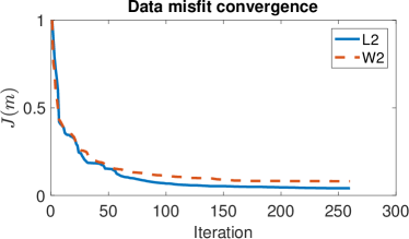
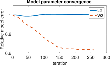
In Figure 10a, both the normalized $L^{2}$ norm and $W_{2}$ distance are reduced from 1 to nearly 0. The plots indicate that $L^{2}$-based inversion does not suffer from local minima in this layered example. The velocity is initiated correctly above the interface. In Figure 10b, $L^{2}$-based inversion has a model convergence curve that is radically different from its data convergence in Figure 10a. The normalized model error, measured by the Frobenius norm of $m_{\text{iter}}-m_{*}$ where $m_{\text{iter}}$ is the reconstruction at the current iteration and $m_{*}$ is the truth, remains unchanged. On the other hand, the $W_{2}$-based inversion has both the $W_{2}$ distance and the model error decreasing rapidly in the first 150 iterations. Since the computational cost per iteration is the same in both cases by computing the $W_{2}$ distance explicitly in 1D [66], the $W_{2}$-based inversion lowers the model error much more quickly. Both the inversion results in Figure 9 and the convergence curves in Figure 10 illustrate that the $W_{2}$-based inversion gives a better reconstruction. Other features of $W_{2}$ other than the convexity for translations and dilations (Theorem 3.1) are playing critical roles in this velocity inversion.

At first glance, it seems puzzling that $W_{2}$-based FWI can even recover velocity in the model where no seismic wave goes through. The fact that there is no reflection from below the known interface in the measured data is, of course, also informative. After analyzing the layered example more carefully, we have summarized two essential properties of the quadratic Wasserstein metric that contribute to the better inversion result, small-amplitude sensitivity and frequency bias.

(a)

(b)

Figure 11: The layered model: (a) $L^{2}$ and (b) $W_{2}$ inversion velocity after 50, 100 and 200 iterations.

Figure 12: Analogy for the true two-layer velocity (solid line), the narrower (dash-dot line) and the wider Wolf ramps (dashed line).

5.3 Small-Amplitude Sensitivity

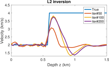
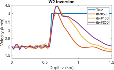
Figure 11a and Figure 11b are the vertical velocity profiles of $L^{2}$-based and $W_{2}$-based FWI at the 50th, 100th and 200th iterations. The inverted velocity profile at the 50th iteration has a gradual transition from 4 km/s back to 2 km/s around $z=1$ km. The simulated reflector is present in the earlier iterations of both $L^{2}$- and $W_{2}$-based inversion. It is often referred to as overshoot. However, this simulated reflector is the key information to uncover the velocity model below the interface.

Although the inverted velocity at 50th iteration does not have the discontinuity at $z=0.6$ km as in the true velocity, there is an frequency-dependent reflectivity caused by the linear velocity transition zone from $z=0.5$ km to $z=1$ km. In 1937, Alfred Wolf [63] first analyzed this particular type of reflectivity dispersion. We extract the linear transition zones and create the analogous versions in Figure 12. The solid plot in Figure 12 represents our target model, while the dashed plots are two types of Wolf ramps, similar to the velocity profiles at the 50th and the 100th iteration in Figure 11.

All three velocity models in Figure 12 produce strong reflections of the same phase, due to the jump in velocity at $z=1$ km. However, the energy reflected is relatively smaller from the ones with Wolf ramps. In addition to that, the linear transition zone generates another reflection which has extremely small energy. If the amplitude of the difference in reflection is $\varepsilon$, the $L^{2}$ misfit is $\mathcal{O}(\varepsilon^{2})$ while the $W_{2}$ misfit is $\mathcal{O}(\varepsilon)$. Since the reflection amplitude $\varepsilon\ll 1$, the $W_{2}$ metric measures the misfit $\mathcal{O}(\varepsilon)\gg\mathcal{O}(\varepsilon^{2})$. Consequently, $W_{2}$-based inversion can correct the velocity model furthermore based on the relatively bigger residual.

(a) Reflections from the narrow Wolf ramp

(b) Reflections from the wide Wolf ramp

Figure 13: Reflections produced by the 3hz and the 7hz Ricker wavelets from the (a) narrow and (b) wide Wolf ramps in Figure 12.

5.4 Frequency Bias

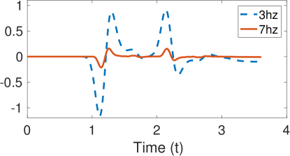
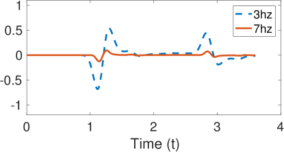
As illustrated in [28, Figure 2], the amplitude of the Wolf ramp reflection coefficient at the normal incident is bigger for lower frequencies and smaller for higher frequencies. This is also observed in Figure 13. The difference between the true data reflection and the one from Wolf ramps is more significant for 3Hz data than the 7Hz one. When the simulated data and the observed data are sufficiently close to each other, inverse matching with the quadratic Wasserstein metric can be viewed as the weighted $\dot{H}^{-1}$ seminorm [40, 15] which has a $1/\mathbf{k}$ weighting on the data spectrum with $\mathbf{k}$ representing the wavenumber. As a result, the $W_{2}$ objective function “sees” more of the stronger low-frequency reflections caused by the Wolf Ramp than the $L^{2}$ norm. Based on its better sensitivity to the low-frequency modes, the $W_{2}$-based inversion can keep updating the velocity model and reconstruct the second layer in Figure 9a by minimizing the “seen” data misfit.

(a) $||m^{\text{low}}_{\text{iter}}-m^{\text{low}}_{*}||_{F}$

(b) $||m^{\text{high}}_{\text{iter}}-m^{\text{high}}_{*}||_{F}$

(c) $||f^{\text{low}}_{\text{iter}}-g^{\text{low}}||_{2}$

(d) $||f^{\text{high}}_{\text{iter}}-g^{\text{high}}||_{2}$

Figure 14: (a) Low-wavenumber and (b) high-wavenumber model convergence; (c) low-frequency and (d) high-frequency $2$-norm data residual for $L^{2}$-based and $W_{2}$-based inversion.

(a) $L^{2}$-FWI at iteration 0

(b) $L^{2}$-FWI at iteration 100

(c) $L^{2}$-FWI at iteration 200

(d) $W_{2}$-FWI at iteration 0

(e) $W_{2}$-FWI at iteration 100

(f) $W_{2}$-FWI at iteration 200

Figure 15: Three-layer model: the residual spectrum for $L^{2}$-based and $W_{2}$ based inversion at iteration 0, 100 and 200.

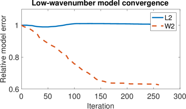
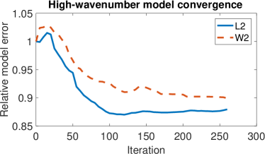
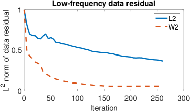
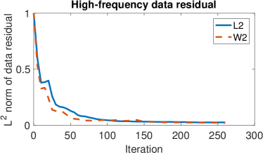
In Figure 10b, we observe that the $2$-norm of the model error in $L^{2}$-based inversion barely changes. We decompose all velocity models in the experiment into low-wavenumber (with Fourier modes $|\mathbf{k}|\leq 30$) and high-wavenumber (with Fourier modes $|\mathbf{k}|>30$ ) parts by bandpass filters. We are interested in the model error decay of each part in the inversion. Similarly, we divide the data residual of both inversions into the low- and high-frequency parts. The residual is computed as the difference between synthetic data $f(\mathbf{x},t;m)$ generated by the model $m$ at current iteration and the true data $g(\mathbf{x},t)$:

$$\text{residual}=f(\mathbf{x},t;m)-g(\mathbf{x},t).$$

The differences between the two objective functions are more clear in Figure 14, which illustrates different convergence patterns for the smooth and oscillatory parts of both the model and the data. The low-wavenumber model error (Figure 14a) and the low-frequency data residual (Figure 14c) of the $W_{2}$-based inversion decreases much more rapidly than the $L^{2}$-based inversion, while the latter shows sensitivity in reducing the high-wavenumber model error and high-frequency residuals, based on Figure 14b and Figure 14d.

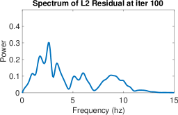
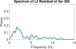
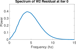
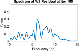
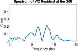
Another way of analyzing the error reduction with respect to different objective functions is to look at their data residual in the Fourier domain. Figure 15 consists of six plots of the residual spectrum of two inversion schemes at three different iterations. By comparing the change of spectrum as the iteration number increases, one can observe that the inversion driven by $L^{2}$ norm has a different pattern in changing the residual spectrum with the $W_{2}$-based inversion. It focuses on reducing the high-frequency residual in early iterations and slowly decreasing the low-frequency residual later. On the other hand, inversion using the $W_{2}$ metric reduces the smooth parts of the residual first (Figure 15e) and then gradually switches to the oscillatory parts (Figure 15f).

The fact that $W_{2}$ is more robust than $L^{2}$ in reconstructing low-wavenumber components while $L^{2}$-FWI converges faster and achieves higher resolution for the high-wavenumber features was already observed in [66], in an inversion example with difficulties of local minima. For the two-layer example discussed above, the $L^{2}$-based inversion does not suffer from local minima trapping, but the properties for these two inversion schemes still hold. Rigorous analysis has been done in [15], where the $L^{2}$ norm and the $W_{2}$ metric were discussed under both the asymptotic and non-asymptotic regimes for data comparison. Theorems have demonstrated that $L^{2}$ norm is good at achieving high resolution in the reconstruction, while the $W_{2}$ metric gives better stability with respect to data perturbation. Using $W_{2}$-based inversion to build a good starting model for the $L^{2}$-based inversion in a later stage is one way to combine useful features of both methods.

6 Numerical Examples

In this section, we demonstrate several numerical examples under both synthetic and somewhat more realistic settings. We will see applications of the $W_{2}$ convexity analysis in Section 3, and more importantly, other improvements in Section 5 that are beyond local-minima trapping. The $L^{2}$ norm and the $W_{2}$ metric will be used as the objective function, and their inversion results will be compared. In particular, we stick with the so-called trace-by-trace approach (8) for inversions using the $W_{2}$ metric.

6.1 The Marmousi Model

The true velocity of the Marmousi model is presented in Figure 16a, which was created to produce complex seismic data that require advanced processing techniques to obtain a correct Earth image. It has become a standard benchmark for methods and algorithms for seismic imaging since 1988 [56]. The initial model shown in Figure 16b lacks all the layered features. We will invert the Marmousi model numerically using the $L^{2}$ norm and the $W_{2}$ metric under one synthetic setting and a more realistic setting in terms of the observed true data.

6.1.1 Synthetic Setting

Under the same synthetic setting, the true data and the synthetic data are generated by the same numerical scheme. The wave source is a 10 Hz Ricker wavelet. A major challenge for the $L^{2}$-based inversion is the phase mismatches in the data generated by the true and initial velocities. After 300 L-BFGS iterations, the $L^{2}$-based inversion converges to a local minimum, as shown in Figure 16c, which is also a sign of cycle skipping due to the lack of convexity with respect to data translation. The $W_{2}$-based inversion, on the other hand, recovers the velocity model correctly, as seen in Figure 16d. As discussed in Section 3, the $W_{2}$ metric has the important convexity with respect to data translation and dilation. Hence, the initial model is within the basin of attraction for the $W_{2}$-based inversion. Once the background velocity is correctly recovered, the missing high-wavenumber features can also be reconstructed correctly.

6.1.2 A More Realistic Setting

For field data inversions, source approximation, the elastic effects, anisotropy, attenuation, noisy measurement, and many other factors could bring modeling errors to the forward propagation. To discuss the robustness of the $W_{2}$-based method with respect to the accuracy of the source estimation and the noise in the measurements, we present another test with more challenging settings.

(a) True velocity

(b) Initial velocity

(c) $L^{2}$ inversion

(d) $W_{2}$ inversion

(e) $L^{2}$ inversion (with noise)

(f) $W_{2}$ inversion (with noise)

Figure 16: The Marmousi model inversion: (a) the true and (b) initial velocities; (c)(d): the $L^{2}$ and $W_{2}$ inversion results for the synthetic setting; (e)(f): the $L^{2}$ and $W_{2}$ inversion results for the realistic setting. We use the linear scaling (2) as the data normalization to calculate the $W_{2}$ metric. All axes are associated with the unit km.

(a) Noise in the data

(b) Estimation of the source wavelet

Figure 17: The realistic setting for the Marmousi model: (a) noisy and clean observed datasets comparison at one trace; (b) estimation of the source wavelet by the linear waveform inversion.

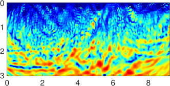
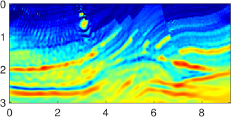
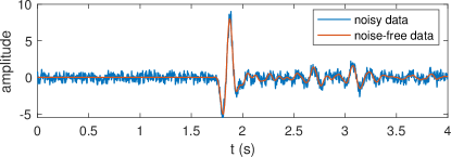
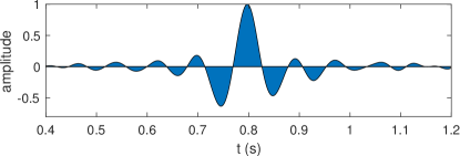
The observed data is generated by a Ricker wavelet centered at 10 Hz as in the previous test, which is additionally polluted by mean-zero correlated random noise; see an illustration of the noisy data in Figure 17a. We estimate the source profile by linear least-squares waveform inversion of the direct wave [44, 48]. A homogeneous medium of $1.5$ km/s is used as the velocity model in the linear inversion. The reconstructed source wavelet is shown in Figure 17b. Inversion results are illustrated in Figure 16e and Figure 16f. The presence of noise and the inaccurate wave source deteriorates the $L^{2}$ result, but only mildly change the $W_{2}$-based inversion. Most structures are recovered with relatively lower resolution. Inaccuracies are present for the shallow part. Nevertheless, in comparison, the $W_{2}$ metric is more robust than the $L^{2}$ norm for small perturbations in the data that come from modeling error or measurement noise.

6.1.3 The Scaling Method

In the $W_{2}$-based Marmousi model inversions, we transform the wavefields into probability densities by the linear scaling (2). The constant $c$ is chosen to be the $\ell^{\infty}$ norm of the observed data. Although the normalized $W_{2}$ metric lacks strict convexity in terms of data translations as we have pointed out in [17], the linear scaling still works remarkably well in practice for most cases, including the realistic inversions in the industry. Also, normalization methods (3) and (4) give similar results and are therefore not included. Nevertheless, data normalization is an important step for $W_{2}$-based full-waveform inversion. More analysis and discussions are presented in Section 4.

It is observed here and in many other works on optimal transport-based FWI that a slight improvement in the convexity of the misfit function seems to produce significant effects on the inversion in mitigating cycle-skipping issues [66, 37]. It is also the case for the linear scaling (2). The linear scaling does not preserve the convexity of the $W_{2}$ metric with respect to translation, but as a sign of improvement, the basin of attraction is larger than the one for the $L^{2}$ norm, as shown previously in Figure 2c and Figure 5a. We can point to three reasons that may contribute to the success of the linear scaling in practice. First, as discussed in Section 4, adding a constant to the signals before being compared by the $W_{2}$ metric brings the Huber effect for better robustness with respect to outliers. Second, it smooths the FWI gradient and thus emphasizes the low-wavenumber components of the model parameter. Third, the convexity with respect to signal translation only covers one aspect of the challenges in realistic inversions. The synthetic data is rarely a perfect translation of the observed data in practice. The nonconvexity caused by the linear scaling might not be an issue in realistic settings, while the outstanding benefits of adding a positive constant dominate.

6.2 The Circular Inclusion Model

We have presented the Marmousi model to demonstrate that $W_{2}$-based inversion is superior to $L^{2}$. We also show that the linear scaling (2) is often good enough as a normalization method. However, to address the importance of data normalization in applying optimal transport, we create a synthetic example in which the linear scaling (2) affects the global convexity of $W_{2}$.

We want to demonstrate the issues above with a circular inclusion model in a homogeneous medium (with $6$ km in width and $4.8$ km in depth). It is also referred to as the “Camembert” model [19]. The true velocity is shown in Figure 18a, where the anomaly in the middle has wave speed $4.6$ km/s while the rest is $4$ km/s. The initial velocity we use in the inversion is a homogeneous model of $4$ km/s. We have 13 sources of 10 Hz Ricker wavelet equally aligned on the top of the domain, while 201 receivers are on the bottom. The recorded signals contain mainly transmissions, which are also illustrated in Figure 1 as an example of the cycle-skipping issues. Figure 1c shows the initial data fit, which is the difference between the observed data and the synthetic data generated by the initial velocity model. As seen in Figure 18b, the inversion with the $L^{2}$ norm as the objective function suffers from local minima trapping.

(a) True velocity

(b) $L^{2}$ inversion

(c) $W_{2}$, square

(d) $W_{2}$, linear

(e) $W_{2}$, exponential

(f) $W_{2}$, softplus

Figure 18: Velocity model with circular inclusion: (a) True velocity; (b) $L^{2}$ inversion; (c)-(f): $W_{2}$-based inversion using the square, the linear, the exponential ($b=0.2$) and the softplus scaling ($b=0.2$).

(a) $L^{2}$ inversion

(b) $W_{2}$, square

(c) $W_{2}$, linear

(d) exponential

(e) $W_{2}$, softplus

Figure 19: Circular inversion: the data fit in the final models for the $L^{2}$ inversion and the $W_{2}$ inversions with the square, linear, exponential, and softplus scalings. All figures are plotted under the same colormap. The initial data fit is presented in Figure 1c.

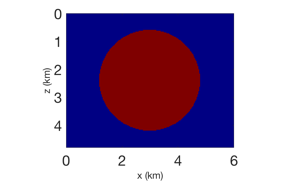
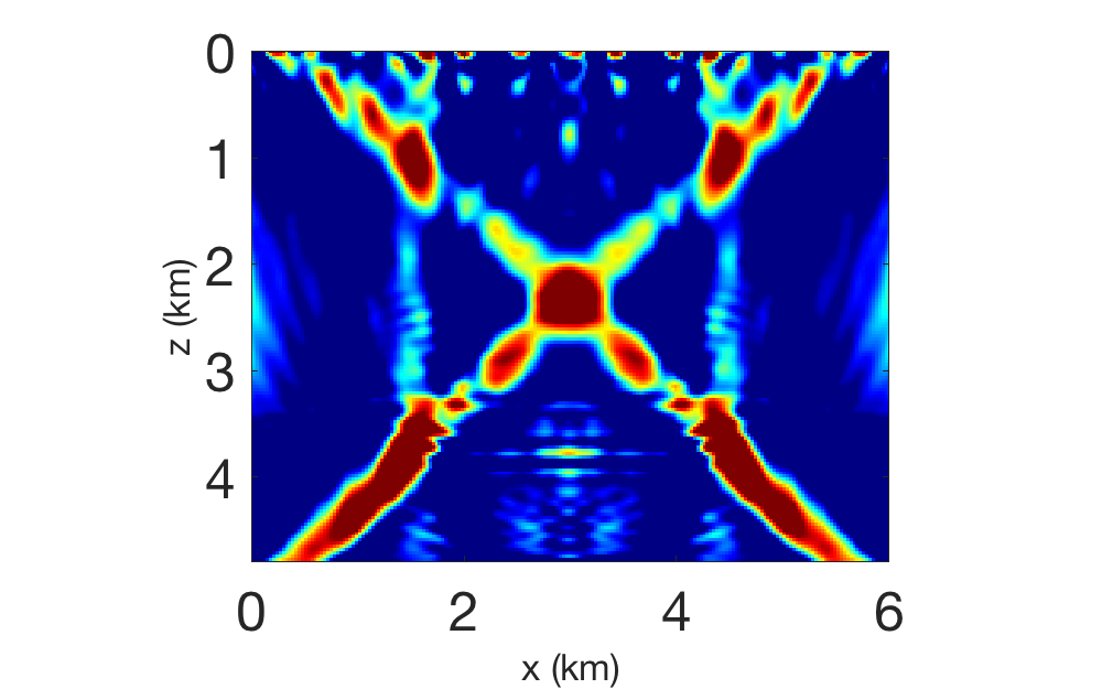
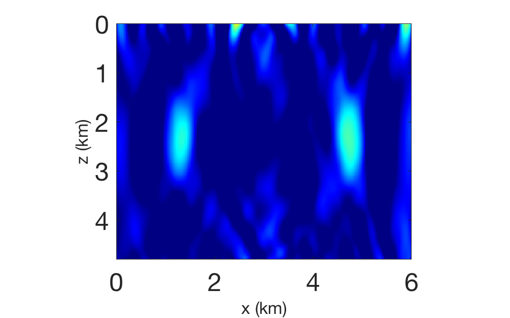
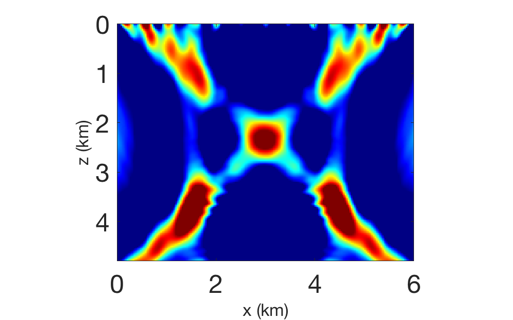
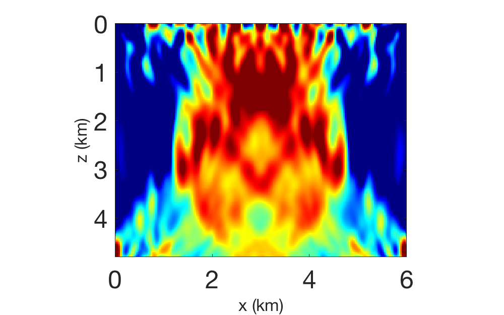
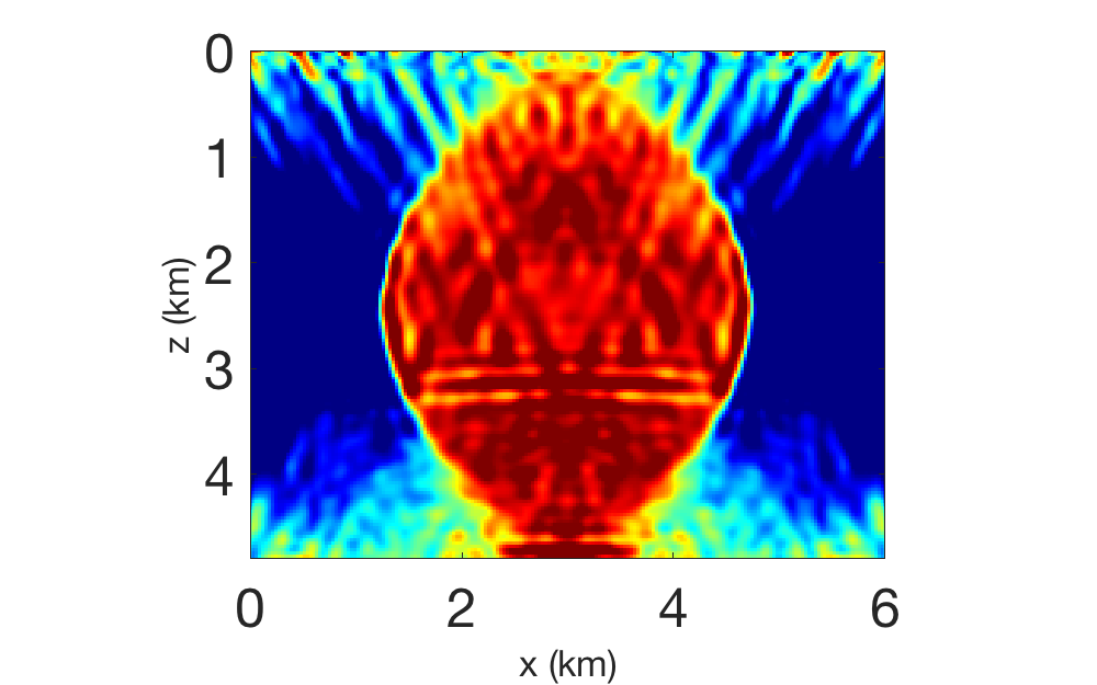
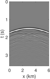
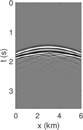
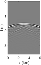
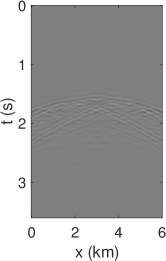
Figure 18c to Figure 18f present inversion results by using the $W_{2}$ metric as the objective function, but with different data normalization methods: the square scaling [17], the linear scaling $\sigma_{l}$, the exponential scaling $\sigma_{e}$, and the softplus scaling $\sigma_{s}$, respectively. As shown in Figure 18c and Figure 18d, $W_{2}$-based inversion under the square scaling and the linear scaling also suffer from cycle-skipping issues whose final inversion results share similarities with the reconstruction by the $L^{2}$ norm. Theoretically, the $W_{2}$ metric is equipped with better convexity, but the data normalization step may weaken the property if an improper scaling method is used. On the other hand, the exponential scaling and the softplus scaling can keep the convexity of the $W_{2}$ metric when applied to signed functions. The additional hyperparameter $b$ in the scaling functions helps to preserve the convexity; see Corollary 4.4 and the discussions in Section 4.2.

Exponential functions amplify both the signal and the noise significantly, making the softplus scaling a more stable method, especially when applied with the same hyperparameter $b$. In this “Camembert model”, Figure 18f with the softplus scaling and $b=0.2$ is the closest to the truth, while Figure 18e by the exponential scaling with $b=0.2$ lacks good resolution around the bottom part. All the figures are plotted under the same color scale. We think data normalization is the most important issue for optimal transport based seismic inversion. We have devoted the entire Section 4 to this important topic, and more developments in the optimal transport theory are necessary to ultimately resolve the issue.

Finally, we present the data misfit of the converged models in Figure 19, which are the differences between the observed data and the synthetic data at convergence from different methods. Compared with the initial data fit in Figure 1c, the square scaling for the $W_{2}$ inversion hardly fits any data, while inversions with the $L^{2}$ norm and the linear scaling reduce partial initial data residual. The exponential and the softplus scaling are better in performance, while the latter stands out for the best data fitting under the setup of this experiment.

(a) Adjoint sources comparison at one trace

(b) Detailed view inside the red box in (a)

Figure 20: Circular inversion: comparison of normalized adjoint sources (the Fréchet derivative of the objective function with respect to the synthetic data) at the first iteration for the $L^{2}$ inversion, the $W_{2}$ inversion with the square, linear, exponential, and softplus scalings.

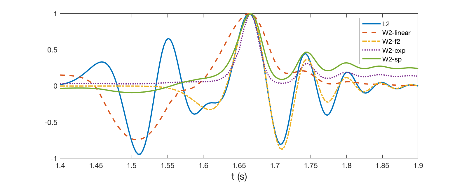
In Figure 20, we compare the adjoint source of different methods at the first iteration. To better visualize the differences, we focus on one of the traces and zoom into the wave-type features. The $L^{2}$ adjoint source is simply the difference between the observed and the synthetic signals, while the one by the linear scaling is closer to its envelope. The enhancement in the low-frequency contents matches our analysis in Section 4. It also partially explains why the linear scaling alone is often observed to mitigate the cycle-skipping issues effectively. The adjoint source by the square scaling has the oscillatory features of the seismic data. The exponential and the softplus scaling methods share similar adjoint sources at the first iteration of the inversion.

Remark 6.1.

Although inversion with the linear scaling fails in the “Camembert” example, it often works well in realistic cases where the recorded data contain various types of seismic waveforms; for example, see Figure 9d and Figure 16d. For cases where the linear scaling struggles, one can turn to the softplus scaling [46], as shown in Figure 18. With properly chosen hyperparameters, the softplus scaling keeps the convexity of the $W_{2}$ metric, which we proved in Corollary 4.4. Hence, the inversion process does not suffer from cycle-skipping issues.

6.3 The Salt Model

In this section, we invert a more realistic model problem, which represents the challenging deep-layer reconstruction with reflections. It is an application of other improvements of the $W_{2}$-based inversion discussed in Section 5 that are beyond tackling local minima.

(a) The original, low-pass filtered and high-pass filtered true velocity

(b) The original, low-pass filtered and high-pass filtered initial velocity

Figure 21: Salt reconstruction: (a) the true and (b) the initial velocity.

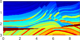
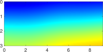
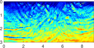
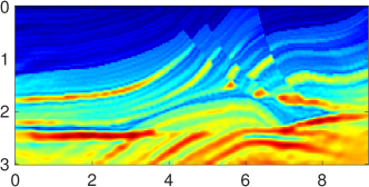
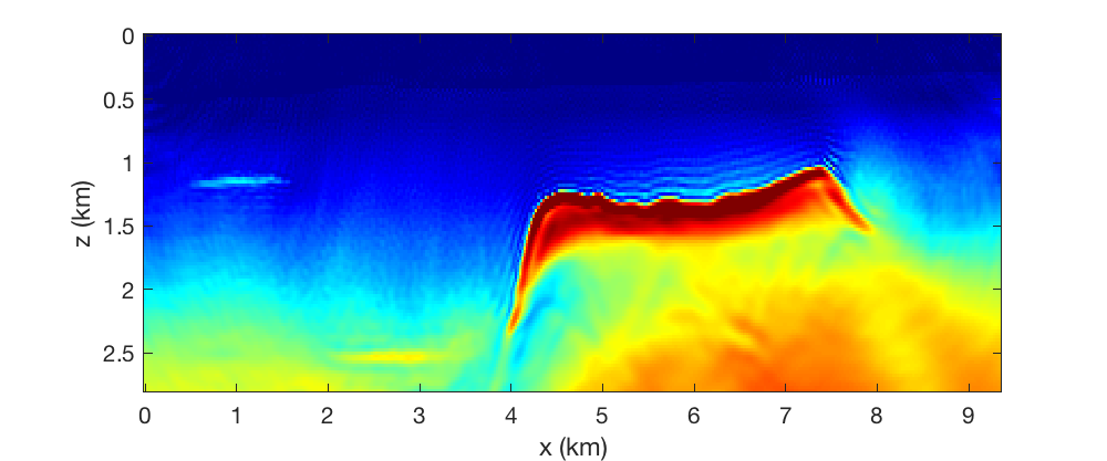
We consider Figure 21a as the true velocity model, which is also part of the 2004 BP benchmark (2.8 km in depth and 9.35 km in width). The model is representative of the complex geology in the deep-water Gulf of Mexico. The main challenges in this area are obtaining a precise delineation of the salt and recovering information on the sub-salt velocity variations [3]. All figures displayed here contain three parts: the original, the low-pass, and high-pass filtered velocity models.

The well-known velocity model with strongly reflecting salt inclusion can be seen as a further investigation of Section 5 in a more realistic setting. The inversion results from these sharp discontinuities in velocity are the same as the layered model in Section 5. With many reflections and refraction waves contributing to the inversion in the more realistic models, it is harder to determine the most relevant mechanisms. Different from the layered example in Section 5, the observed data here contains diving waves, which are wavefronts continuously refracted upwards through the Earth due to the presence of a vertical velocity gradient. However, reflections still carry the essential information of the deep region in the subsurface and are the driving force in the salt inclusion recovery.

6.3.1 The Synthetic Setting

The inversion starts from an initial model with the smoothed background without the salt (Figure 21b). We place 11 sources of 15 Hz Ricker wavelet and 375 receivers equally on the top. The total recording time is 4 seconds. The observed data is dominated by the reflection from the top of the salt inclusion. After 100 iterations, FWI using both objective functions can detect the salt upper boundary. Figure 22a and Figure 22b also show that the high-wavenumber components of the velocity models are partially recovered in both cases, while the smooth components barely change. This is different from the Marmousi example, where high-wavenumber components cannot be correctly recovered ahead of the smooth modes.

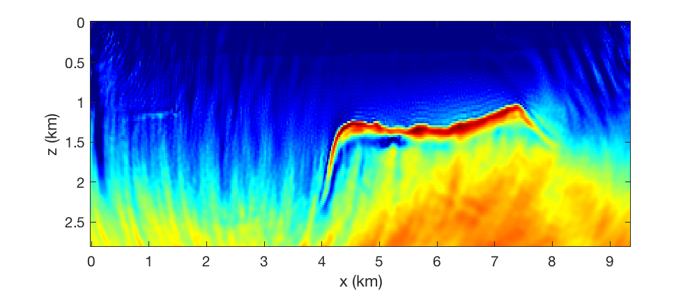
With more iterations, the $W_{2}$-based inversion gradually recovers most parts of the salt body (Figure 23b), which is much less the case for $L^{2}$-based inversion, as shown in Figure 23a. In particular, one can observe that a wrong sublayer is created after 600 L-BFGS iterations in Figure 23a from which one may have a misleading interpretation about the Earth. Figure 23b matches the original salt body. In general, features related to the salt inclusion can be better determined by using optimal transport-related metrics as the misfit function with the help of both refraction and reflection; also see [65, Figure 4] for example.

(a) The original, low-pass filtered and high-pass filtered $L^{2}$-FWI after 100 iterations

(b) The original, low-pass filtered and high-pass filtered $W_{2}$-FWI after 100 iterations

Figure 22: Salt reconstruction: (a)the $L^{2}$-based and (b) $W_{2}$-based inversion after 100 L-BFGS iterations.

(a) The original, low-pass filtered and high-pass filtered $L^{2}$-FWI after 600 iterations

(b) The original, low-pass filtered and high-pass filtered $W_{2}$-FWI after 600 iterations

Figure 23: Salt reconstruction: (a)the $L^{2}$-based and (b)) $W_{2}$-based inversion after 600 L-BFGS iterations.

(a) Comparison between the clean data and the noisy data

(b) $L^{2}$-based inversion

(c) $W_{2}$-based inversion

Figure 24: Salt reconstruction under the realistic setting: (a) the comparison between the clean data and the noisy data, which is also generated by a refined mesh (b) $L^{2}$-based inversion and (c) $W_{2}$-based inversion after convergence.

6.3.2 A More Realistic Setting

Similar to Section 6.1.2, we present another test where a refined finite-difference mesh simulates the observed data, and thus a different wave propagator is used in this inversion test. Additionally, the reference data contains correlated mean-zero noise. Other setups remain the same. Figure 24a compares samples of the (noisy) observed data used in this test and the one in the previous test. Figure 24b is the inversion using the $L^{2}$ norm as the objective function, while Figure 24c presents the inversion results based on the $W_{2}$ metric where the linear scaling (2) is used to normalize the signals. Both tests are stopped after the L-BFGS algorithm can no longer find a feasible descent direction. With the presence of noise, both methods correctly reconstruct the upper boundary of the salt body based on the phase information of the reflections. However, amplitudes of the wave signals are corrupted by the noise, which affects the reconstruction of the entire salt body.

The $W_{2}$-based inversion with the noisy data can still recover a significant amount of the salt body. However, the thickness of the layer is smaller than the one from the synthetic setting (Figure 23b). It is expected based on our discussion on the small-amplitude sensitivity in Section 5.3. The energy reflected by the upper boundary of the salt is minimal, but it is critical for the $W_{2}$ metric to reconstruct the model features below the reflecting interface in the previous synthetic setting. The small reflection can be obscured by the presence of noise and modeling error under this realistic setting.

Nevertheless, the $W_{2}$-based reconstruction has almost no footprint from the noise except the salt body, while the $L^{2}$-based inversion has a distinct noise pattern; see Figure 24b. It is an interesting phenomenon observed from all numerical tests of $W_{2}$-based inversion. Instead of over-fitting the noise or the wrong information in the data, $W_{2}$-based inversion stops with no feasible descent direction, while $L^{2}$-based inversion continues updating the model parameter, but mainly fits the noise and numerical errors which in turn gives noisy and incorrect reconstructions. It is another demonstration of the good stability of the $W_{2}$ metric for data-fitting problems, as discussed in [15].

7 Conclusion

In this paper, we have analyzed several favorable new properties of the quadratic Wasserstein distance connected to seismic inversion, compared to the standard $L^{2}$ techniques. We have presented a sharper convexity theorem regarding both translation and dilation changes in the signal. The improved theorem offers a more solid theoretical foundation for the wide range of successful field data inversions conducted in the exploration industry. It shows why trapping in local minima, the so-called cycle skipping, is avoided, and the analysis gives guidance to algorithmic developments.

Data normalization is a central component of the paper. It has always been a limitation for optimal transport applications, including seismic imaging, which needs to compare signed signals where the requirement of non-negativity and the notion of equal mass are not natural. We study different normalization methods and define a class with attractive properties. Adding a buffer constant turns out to be essential. In a sequence of theorems, we show that the resulting relevant functional for optimization is a metric, and the normalized signals are more regular than the original ones. We also prove a Huber-norm type of property, which reduces the influence of seismic events that are far apart and should not affect the optimization. The analysis here explains the earlier contradictory observations [66] that linear normalization often worked better in applications than many other scaling methods, even if it lacks convexity with respect to shifts [17].

The final contribution of the paper is to present and analyze the remarkable capacity of the $W_{2}$-based inversion of sublayer recovery with only the reflection data even when there is no seismic wave returning to the surface from this domain. The conventional $L^{2}$ norm does not perform well, and here it is not the issue of cycle skipping. Both amplitude and frequency play a role. Compared to the $W_{2}$ metric, the $L^{2}$ norm lacks sensitivity to small-amplitude signals. We saw this in numerical tests and from classical refraction analysis. The inherent insensitivity of the $L^{2}$ norm to low-frequency contents of the residual is a primary reason behind the fact that $L^{2}$-FWI often fails to recover the model kinematics. $W_{2}$-based inversion captures the essential low-frequency modes of the data residual, directly linked to the low-wavenumber structures of the velocity model. This property is important for applications of this type, where the initial model has poor background velocity.

With this paper, the mathematical reasons for the favorable properties of $W_{2}$-based inversion become quite clear. There are still several other issues worth studying that could have important practical implications. Examples are further analysis of other forms of optimal transport techniques as, for example, unbalanced optimal transport and $W_{1}$. The scalar wave equation is the dominating model in practice, but elastic wave equations and other more realistic models are gaining ground, and extending the analysis and best practices to these models will be essential.

References

- [1] Ambrosio, L.; Gigli, N. A user’s guide to optimal transport. in Modelling and Optimisation of Flows on Networks, pp. 1–155, Springer, 2013.
- [2] Ambrosio, L.; Mainini, E.; Serfaty, S. Gradient flow of the Chapman-Rubinstein-Schatzman model for signed vortices. Ann. Inst. H. Poincaré Anal. Non Linéaire 28 (2011), no. 2, 217–246.
- [3] Billette, F.; Brandsberg-Dahl, S.: The 2004 BP velocity benchmark, in 67th EAGE Conference & Exhibition, European Association of Geoscientists & Engineers, 2005 pp. cp–1.
- [4] Brenier, Y. Polar factorization and monotone rearrangement of vector-valued functions. Comm. Pure Appl. Math. 44 (1991), no. 4, 375–417.
- [5] Caffarelli, L. A. The regularity of mappings with a convex potential. J. Amer. Math. Soc. 5 (1992), no. 1, 99–104.
- [6] Cao, Y.; Li, S.; Petzold, L.; Serban, R. Adjoint sensitivity analysis for differential-algebraic equations: The adjoint DAE system and its numerical solution. SIAM J. Sci. Comput. 24 (2003), no. 3, 1076–1089.
- [7] Chavent, G. Nonlinear least squares for inverse problems: theoretical foundations and step-by-step guide for applications, Springer Science & Business Media, 2010.
- [8] Chavent, G.; Dupuy, M.; Lemmonier, P. History matching by use of optimal control theory. Society of Petroleum Engineers Journal 15 (1975), no. 01, 74–86.
- [9] Chen, J.; Chen, Y.; Wu, H.; Yang, D. The quadratic Wasserstein metric for earthquake location. J. Comput. Phys. 373 (2018), 188–209.
- [10] Chizat, L.; Peyré, G.; Schmitzer, B.; Vialard, F.-X. Unbalanced optimal transport: Dynamic and Kantorovich formulation. J. Funct. Anal. 274 (2018), no. 11, 3090–3123.
- [11] Demanet, L. Class Notes for Topics in Applied Mathematics: Waves and Imaging. MIT Course Number 18.325 (2016).
- [12] Engquist, B.; Froese, B. D. Application of the Wasserstein metric to seismic signals. Commun. Math. Sci. 12 (2014), no. 5, 979–988.
- [13] Engquist, B.; Froese, B. D.; Yang, Y. Optimal transport for seismic full waveform inversion. Commun. Math. Sci. 14 (2016), no. 8, 2309–2330.
- [14] Engquist, B.; Majda, A. Absorbing boundary conditions for numerical simulation of waves. Proc. Natl. Acad. Sci. USA 74 (1977), no. 5, 1765–1766.
- [15] Engquist, B.; Ren, K.; Yang, Y. The quadratic Wasserstein metric for inverse data matching. Inverse Problems 36 (2020), no. 5, 055 001.
- [16] Engquist, B.; Yang, Y. Seismic imaging and optimal transport. Commun. Inf. Syst. 19 (2019), no. 2, 95–145.
- [17] Engquist, B.; Yang, Y. Seismic inversion and the data normalization for optimal transport. Methods Appl. Anal. 26 (2019), no. 2, 133–148.
- [18] Gangbo, W.; Li, W.; Osher, S.; Puthawala, M. Unnormalized optimal transport. J. Comput. Phys. 399 (2019), 108 940.
- [19] Gauthier, O.; Virieux, J.; Tarantola, A. Two-dimensional nonlinear inversion of seismic waveforms: Numerical results. Geophysics 51 (1986), no. 7, 1387–1403.
- [20] Glorot, X.; Bordes, A.; Bengio, Y.: Deep sparse rectifier neural networks, in Proceedings of the fourteenth international conference on artificial intelligence and statistics, 2011 pp. 315–323.
- [21] Huber, P. J. Robust regression: asymptotics, conjectures and Monte Carlo. Ann. Statist. 1 (1973), no. 5, 799–821.
- [22] Jannane, M.; Beydoun, W.; Crase, E.; Cao, D.; Koren, Z.; Landa, E.; Mendes, M.; Pica, A.; Noble, M.; Roeth, G.; et al. Wavelengths of earth structures that can be resolved from seismic reflection data. Geophysics 54 (1989), no. 7, 906–910.
- [23] Kantorovich, L. V. Mathematical methods of organizing and planning production. Management Science 6 (1960), no. 4, 366–422.
- [24] Knott, M.; Smith, C. S. On the optimal mapping of distributions. J. Optim. Theory Appl. 43 (1984), no. 1, 39–49.
- [25] Kolouri, S.; Park, S.; Thorpe, M.; Slepčev, D.; Rohde, G. K. Transport-based analysis, modeling, and learning from signal and data distributions. arXiv preprint arXiv:1609.04767 (2016).
- [26] Lailly, P.: The seismic inverse problem as a sequence of before stack migrations, in Conference on Inverse Scattering: Theory and Application, Society for Industrial and Applied Mathematics, Philadelphia, PA, 1983 pp. 206–220.
- [27] Lellmann, J.; Lorenz, D. A.; Schonlieb, C.; Valkonen, T. Imaging with Kantorovich–Rubinstein discrepancy. SIAM J. Imaging Sci. 7 (2014), no. 4, 2833–2859.
- [28] Liner, C. L.; Bodmann, B. G. The Wolf ramp: Reflection characteristics of a transition layer. Geophysics 75 (2010), no. 5, A31–A35.
- [29] Liu, D. C.; Nocedal, J. On the limited memory BFGS method for large scale optimization. Math. Program. 45 (1989), no. 1-3, 503–528.
- [30] Mainini, E. A description of transport cost for signed measures. J. Math. Sci. 181 (2012), no. 6, 837–855.
- [31] McCann, R. J. Existence and uniqueness of monotone measure-preserving maps. Duke Math. J. 80 (1995), no. 2, 309–324.
- [32] McGillivray, P. R.; Oldenburg, D. Methods for calculating Fréchet derivatives and sensitivities for the non-linear inverse problem: A comparative study 1. Geophysical prospecting 38 (1990), no. 5, 499–524.
- [33] Messud, J.; Sedova, A.: Multidimensional optimal transport for 3D FWI: demonstration on field data, in 81st EAGE Conference and Exhibition 2019, vol. 2019, European Association of Geoscientists & Engineers, 2019 pp. 1–5.
- [34] Métivier, L.; Allain, A.; Brossier, R.; Mérigot, Q.; Oudet, E.; Virieux, J. Optimal transport for mitigating cycle skipping in full-waveform inversion: A graph-space transform approach. Geophysics 83 (2018), no. 5, R515–R540.
- [35] Métivier, L.; Brossier, R.; Merigot, Q.; Oudet, E. A graph space optimal transport distance as a generalization of distances: application to a seismic imaging inverse problem. Inverse Problems 35 (2019), no. 8, 085 001.
- [36] Métivier, L.; Brossier, R.; Mérigot, Q.; Oudet, E.; Virieux, J. Measuring the misfit between seismograms using an optimal transport distance: application to full waveform inversion. Geophysical Journal International 205 (2016), no. 1, 345–377.
- [37] Métivier, L.; Brossier, R.; Mérigot, Q.; Oudet, E.; Virieux, J. An optimal transport approach for seismic tomography: application to 3D full waveform inversion. Inverse Problems 32 (2016), no. 11, 115 008.
- [38] Monge, G. Mémoire sur la théorie des déblais et de remblais. Histoire de l’académie royale des sciences de paris, avec les Mémoires de Mathématique et de Physique pour la même année (1781), 666–704.
- [39] Peyré, G.; Cuturi, M. Computational optimal transport. Foundations and Trends in Machine Learning 11 (2019), no. 5-6, 355–607.
- [40] Peyre, R. Comparison between distance and norm, and localization of Wasserstein distance. ESAIM Control Optim. Calc. Var. (2018).
- [41] Pladys, A.; Brossier, R.; Irnaka, M.; Kamath, N.; Métivier, L. Assessment of optimal transport based FWI: 3D OBC Valhall case study. in SEG Technical Program Expanded Abstracts 2019, pp. 1295–1299, Society of Exploration Geophysicists, 2019.
- [42] Plessix, R.-E. A review of the adjoint-state method for computing the gradient of a functional with geophysical applications. Geophysical Journal International 167 (2006), no. 2, 495–503.
- [43] Poncet, R.; Messud, J.; Bader, M.; Lambaré, G.; Viguier, G.; Hidalgo, C.: Fwi with optimal transport: a 3d implementation and an application on a field dataset, in 80th EAGE Conference and Exhibition 2018, 1, European Association of Geoscientists & Engineers, 2018 pp. 1–5.
- [44] Pratt, R. G.; Worthington, M. Inverse theory applied to multi-source cross-hole tomography. Part 1: Acoustic wave-equation method. Geophysical Prospecting 38 (1990), no. 3, 287–310.
- [45] Puthawala, M. A.; Hauck, C. D.; Osher, S. J. Diagnosing forward operator error using optimal transport. J. Sci. Comput. 80 (2019), no. 3, 1549–1576.
- [46] Qiu, L.; Ramos-Martínez, J.; Valenciano, A.; Yang, Y.; Engquist, B. Full-waveform inversion with an exponentially encoded optimal-transport norm. in SEG Technical Program Expanded Abstracts 2017, pp. 1286–1290, Society of Exploration Geophysicists, 2017.
- [47] Ramos-Martínez, J.; Qiu, L.; Kirkebø, J.; Valenciano, A.; Yang, Y. Long-wavelength FWI updates beyond cycle skipping. in SEG Technical Program Expanded Abstracts 2018, pp. 1168–1172, Society of Exploration Geophysicists, 2018.
- [48] Ribodetti, A.; Operto, S.; Agudelo, W.; Collot, J.-Y.; Virieux, J. Joint ray+ born least-squares migration and simulated annealing optimization for target-oriented quantitative seismic imaging. Geophysics 76 (2011), no. 2, R23–R42.
- [49] Ricker, N. Further developments in the wavelet theory of seismogram structure. Bulletin of the Seismological Society of America 33 (1943), no. 3, 197–228.
- [50] Scarinci, A.; Fehler, M.; Marzouk, Y. Robust bayesian moment tensor inversion using transport-lagrangian distances. in SEG Technical Program Expanded Abstracts 2019, pp. 2123–2127, Society of Exploration Geophysicists, 2019.
- [51] Sun, B.; Alkhalifah, T. The application of an optimal transport to a preconditioned data matching function for robust waveform inversion. Geophysics 84 (2019), no. 6, R923–R945.
- [52] Sun, B.; Alkhalifah, T. Stereo optimal transport of the matching filter. in SEG Technical Program Expanded Abstracts 2019, pp. 1285–1289, Society of Exploration Geophysicists, 2019.
- [53] Tarantola, A. Inversion of seismic reflection data in the acoustic approximation. Geophysics 49 (1984), no. 8, 1259–1266.
- [54] Tarantola, A. Inverse Problem Theory: Methods for Data Fitting and Model Parameter Estimation, SIAM, 2005.
- [55] Thorpe, M.; Park, S.; Kolouri, S.; Rohde, G. K.; Slepčev, D. A transportation distance for signal analysis. J. Math. Imaging Vision 59 (2017), no. 2, 187–210.
- [56] Versteeg, R. The Marmousi experience: Velocity model determination on a synthetic complex data set. The Leading Edge 13 (1994), no. 9, 927–936.
- [57] Villani, C. Topics in Optimal Transportation, Graduate Studies in Mathematics, vol. 58, American Mathematical Society, Providence, RI, 2003.
- [58] Villani, C. Optimal Transport: Old and New, vol. 338, Springer Science & Business Media, 2008.
- [59] Virieux, J.; Asnaashari, A.; Brossier, R.; Métivier, L.; Ribodetti, A.; Zhou, W. An introduction to full waveform inversion. in Encyclopedia of exploration geophysics, pp. R1–1, Society of Exploration Geophysicists, 2017.
- [60] Virieux, J.; Operto, S. An overview of full-waveform inversion in exploration geophysics. Geophysics 74 (2009), no. 6, WCC1–WCC26.
- [61] Vogel, C. R. Computational Methods for Inverse Problems, vol. 23, SIAM, 2002.
- [62] Wang, D.; Wang, P. Adaptive quadratic Wasserstein full-waveform inversion. in SEG Technical Program Expanded Abstracts 2019, pp. 1300–1304, Society of Exploration Geophysicists, 2019.
- [63] Wolf, A. The reflection of elastic waves from transition layers of variable velocity. Geophysics 2 (1937), no. 4, 357–363.
- [64] Wolfe, P. Convergence conditions for ascent methods. SIAM Rev. 11 (1969), no. 2, 226–235.
- [65] Yang, Y.; Engquist, B. Analysis of optimal transport and related misfit functions in full-waveform inversion. Geophysics 83 (2018), no. 1, A7–A12.
- [66] Yang, Y.; Engquist, B.; Sun, J.; Hamfeldt, B. F. Application of optimal transport and the quadratic Wasserstein metric to full-waveform inversion. Geophysics 83 (2018), no. 1, R43–R62.
- [67] Zhou, D.; Chen, J.; Wu, H.; Yang, D.; Qiu, L. The Wasserstein–Fisher–Rao metric for waveform based earthquake location. arXiv preprint arXiv:1812.00304 (2018).