Bayesian Inference for Big Spatial Data Using Non-stationary Spectral Simulation
Abstract
It is increasingly understood that the assumption of stationarity is unrealistic for many spatial processes. In this article, we combine dimension expansion with a spectral method to model big non-stationary spatial fields in a computationally efficient manner. Specifically, we use Mejía and Rodríguez-Iturbe, (1974)’s spectral simulation approach to simulate a spatial process with a covariogram at locations that have an expanded dimension. We introduce Bayesian hierarchical modelling to dimension expansion, which originally has only been modeled using a method of moments approach. In particular, we simulate from the posterior distribution using a collapsed Gibbs sampler. Our method is both full rank and non-stationary, and can be applied to big spatial data because it does not involve storing and inverting large covariance matrices. Additionally, we have fewer parameters than many other non-stationary spatial models. We demonstrate the wide applicability of our approach using a simulation study, and an application using ozone data obtained from the National Aeronautics and Space Administration (NASA).
1 Introduction
There is increasing interest in using spatial statistical methods to model environmental processes. This is partially due to the emergence of remote sensing instruments and the popularity of Geographic Information Systems (GIS) software (e.g. see, Stein et al.,, 2006; Kalkhan,, 2011, for standard references). The main goal of these analyses is to make predictions at observed and unobserved locations and provide uncertainty quantification. Early works make the assumption that the process is weakly stationary (e.g., see Cressie,, 1993, for a review); that is, the covariance between the response at two different locations is a function of the spatial lag. However, non-stationary processes are much more common in environmental systems observed over large heterogeneous spatial domains (see Bradley et al.,, 2016, for a disscussion). There are many models for non-stationary spatial data, and reduced ranks basis function expansions have become a popular choice (Banerjee et al.,, 2008; Cressie and Johannesson,, 2008). However, there are inferential issues with reduced rank methods in the spatial setting (Stein,, 2014), and consequently, there is renewed interest in proposing computationally efficient full-rank models (Nychka et al.,, 2015; Datta et al.,, 2016a; Katzfuss,, 2017; Bradley et al.,, 2018; Katzfuss et al.,, 2018). Thus, in this article our primary goal is to develop an efficient full rank non-stationary spatial statistical model.
There are numerous methods available to model non-stationary spatial data. For example, process convolution (Higdon,, 1998; Paciorek and Schervish,, 2006; Neto et al.,, 2014) convolves a known spatially referenced function with a spatial process typically assumed to be Gaussian. There are several related, but different approaches available. For example, using a finite integral representation of a process convolution results in a basis function expansion (Cressie and Wikle,, 2011, page 157). Several parameterizations of basis function expansions are available, including: fixed rank kriging (Cressie and Johannesson,, 2008), lattice kriging (Nychka et al.,, 2015), the predictive process (Banerjee et al.,, 2008), and a stochastic partial differential equation approach (Lindgren et al.,, 2011), among others.
An alternative to modelling nonstationarity with spatial basis functions is to assume a deformation (Sampson and Guttorp,, 1992). Here, Euclidean space is “deformed,” or warped, so that far away locations can be more correlated, and vice versa. The parameter space for this method is considerably smaller than many parameterizations using spatial basis function expansions (e.g., see Cressie and Johannesson,, 2008; Kang and Cressie,, 2011, for examples), and is full rank. A similar but different approach to deformation is referred to as “dimension expansion” (Bornn et al.,, 2012). This method involves extending the dimension of the locations to a higher dimensional space. This methodology is based on the surprising result that every non-stationary covariance function in can be written as a stationary covariogram defined on locations in (Perrin and Meiring,, 2003). Recently, Bornn et al., (2012) proposed a method of moments approach to analyzing spatio-temporal data using dimension expansion. To our knowledge the dimension expansion approach has not been implemented using a Bayesian framework.
Thus, our first contribution is to introduce dimension expansion to the Bayesian setting to analyze big spatial data. To achieve a computationally efficient approach to dimension expansion in the Bayesian setting we offer three technical results. In our first technical result, we provide a “non-stationary version” of Bochner’s Theorem (Bochner,, 1959). That is, we show that a non-stationary covariance function can be written as a convolution of the cosine function with a spectral density. The proof of this result simply involves combining Perrin and Meiring, (2003)’s dimension expansion result with Bochner’s Theorem. This result opens up new opportunities to use spectral methods to model non-stationary spatial process. Other methods exist (e.g. see, Priestley,, 1965; Martin,, 1982) to model non-stationary data using spectral densities. However, these methods involve difficult to interpret types of “quasi-stationarity” assumptions (see, Sayeed and Jones,, 1995, for a discussion), while our approach can be easily interpreted through dimension expansion. Castruccio and Guinness, (2017) have also proposed an approach that uses evolutionary spectrum and incorporates an axial symmetric structure into their model.
The second technical result developed in this manuscript follows from our non-stationary version of Bochner’s Theorem. Specifically, we extend Mejía and Rodríguez-Iturbe, (1974)’s method for spectral simulation of a stationary spatial processes to non-stationary spatial processes. This makes it straightforward to simulate in the high-dimensional non-stationary setting because spectral simulation does not require the inverse and storage of a high-dimensional covariance matrix (i.e., is matrix free). In practice, Gaussian spatial datasets correspond to a likelihood that is difficult to compute in high dimensions (i.e., when the dimension of the data is large) because this requires computation and dynamic memory.
Our algorithm is a type of collapsed Gibbs sampler (Liu,, 1994) and it involves two steps. The first step is to augment the likelihood with an -dimensional random vector. Then non-stationary spectral simulation is used within each step of Gibbs sampler to simulate this random vector from it’s prior distribution. This strategy is computationally feasible, full-rank, does not require storage of large matrices, and can be implemented on irregularly spaced locations. This last feature is particularly important as spectral methods based on the discrete Fourier transform often require regularly spaced locations (Fuentes,, 2002; Fuentes et al.,, 2008).
The remaining sections of this article are organized as follows. Section 2 introduces our proposed statistical model, and our first two theoretical results. In Section 3, we describe our implementation, which includes inference using a collapsed Gibbs sampler. In Section 4, we present a simulation study, and compare our approach to two different state-of-the art methods in spatial statistics referred to as the Nearest Neighbor Gaussian Process (NNGP; Datta et al.,, 2016b) and the general Vecchia approximation (Katzfuss and Guinness,, 2017). In Section 5, we implement our model using the benchmark ozone dataset analyzed in (Cressie and Johannesson,, 2008) and (Zhang et al.,, 2018). Finally, Section 6 contains a discussion. For ease of exposition all proofs are given in the appendices.
2 Methodology
Let be a spatial process defined for all s, where is the spatial domain of interest in -dimensional Euclidean space, . We observe the value of at a finite set of locations , , . The data is decomposed additively with
where s, is the Gaussian process of principal interest, and the Gaussian process represents measurement error. The measurement error is assumed to be uncorrelated with mean-zero and variance function .
The process is further decomposed as
where is a known -dimensional vector of covariates, and is unknown. For any collection of locations , the random vector is assumed to have the probability density function (pdf),
| (1) |
where is the multivariate normal distribution with mean , covariance matrix , and is an identity matrix. The pdf will be specified in Section 2.2, but is approximately normal with mean zero, and covariance matrix , where the -th element of is
where
, and is a Euclidean distance. This covariance function uses the aforementioned dimension expansion approach from Bornn et al., (2012). Here, is an matrix consisting of known basis functions. This use of spatial basis functions is similar to the model in Shand and Li, (2017). It will be useful to organize the -dimensional vectors , and . To model Z set define the prediction locations such that the observed locations . Define the corresponding diagonal matrix .
2.1 The Bayesian Hierarchical Model
In this section, we summarize the statistical model used for inference. The model is organized using the “data model”, “process model”, and “parameter model” notation used in Cressie and Wikle, (2011), as follows:
| (2) |
In Equation (2), O is an incidence matrix, is a p-dimensional vector of zeros; “” is a shorthand for a multivariate normal distribution with mean and positive definite covariance matrix ; “” is a shorthand for the inverse gamma distribution with shape and scale ; and “” is a shorthand for a uniform distribution with lower bound and upper bound . All hyperparameters are chosen so that the corresponding prior distribution is “flat”. Example specifications are provided in Section 4 and Section 5.
Process Model 1, Parameter 1, and Parameter Models 35 are fairly standard assumptions for Gaussian data, as they lead to easy to sample full-conditional distributions within a Gibbs sampler (Cressie and Wikle,, 2011). Parameter model 6 and 7 are used to avoid identifiability issues and leads to a conjugate full-conditional distribution (see Banerjee et al.,, 2015, page 124). It is common to assume Process Model 2 is is the multivariate normal distribution with mean zero and covariance matrix (Banerjee et al.,, 2015; Cressie and Wikle,, 2011). However, is only approximately normal with mean-zero and covariance matrix (see Section 2.2 for details).
2.2 Theoretical Considerations
A non-stationary extension of Bochner’s Theorem is stated in Theorem 1.
Theorem 1:Let be a positive definite function on , which is assumed to be compact and bounded. Then there exists a function and a measure such that for any pair of locations ,
| (3) |
where the 2d-dimensional vector .
Proof: See Appendix A.
The proof of Theorem 1 involves a simple combination of the result in Perrin and Meiring, (2003) and Bochner’s Theorem. We use Theorem 1 to define a nonstationary covariance function . That is, in our model we choose a specific form for and , and we use Equation (3) to define our nonstationary covariance function.
Additionally, in practice we assume , which is similar to the strategy used in Bornn et al., (2012) and Shand and Li, (2017). This leads naturally to questions on how to specify spatial basis functions. In general, we use radial basis functions with equally spaced knot locations as suggested in Nychka, (2001) and Cressie and Johannesson, (2008). One might also consider the use of information criteria to adaptively select knot locations (Bradley et al.,, 2011; Tzeng and Huang,, 2017).
There are several things we can learn from Theorem 1. First, every non-stationary covariance function can be written as a convolution in 2d-dimensional space according to (3). Second, is a deformation, which shows an explicit connection between dimension expansion and deformation. Furthermore, this deformation induces non-stationarity, since leads to the classical version of Bochner’s Theorem. Third, if we assume a specific form of , we can use Equation (3) to approximate the covariance function. For example, when is the exponential covariance function (as is the case in (2)), then has a corresponding Cauchy density (Stein,, 1999). We provide a discussion and consider several other covariograms. Our empirical results suggest that the results appear robust to the choice of covariogram. Denote the density corresponding to with . Moreover, the ability to simulate from the spectral density without mathematical operations of covariance matries, allows us to completely circumvent computing and storing a covariance matrix (Mejía and Rodríguez-Iturbe,, 1974).
Theorem 2: Let , , and . Then for a given the random process,
| (4) |
, and , and converges in distribution (as ) to a mean-zero Gaussian process with covariance in Equation (3) with spectral density .
Proof: See Appendix A.
The proof of Theorem 2 involves a simple combination of the result in Perrin and Meiring, (2003) and Cressie, (1993, pg. 204). In practice, to use Theorem 2, we need to specify the spectral density. In our implementation, we assume that , where for each , and is the Cauchy density. This choice of the Cauchy density leads to the exponential covariogram (Cressie,, 1993).
It is arguably more common to simulate using a Cholesky decomposition. However, this requires order computation and order memory. Theorem 2 allows us to simulate without these memory and computational problems. It follows from the transformation theorem (Resnick,, 2013) that the pdf of is given, under our specification, by
| (5) |
where is the indicator function. Again, from Cressie, (1993, pg. 204) and Theorem 2 the pdf in (5) is roughly Gaussian with mean zero and covariance .
3 Collapsed Gibbs Sampling
In this section, we outline the steps needed for collapsed Gibbs sampling. Gibbs sampling requires simulating from full-conditional distributions (Gelfand and Smith,, 1990). In a collapsed Gibbs sampler, some of the events conditioned on in the full-conditional distribution are integrated out (Liu,, 1994). For simplicity, we use the bracket notation, where [] represents the conditional distribution of a X given Y for generic random variables X and Y. In Algorithm 1, we present the steps needed for our proposed collapsed Gibbs sampler.
The expressions for the full-conditional distributions listed in Algorithm 1 are derived in Appendix B. This collapsed Gibbs sampler can easily be modified to allow for heterogeneous variances, and allow for other choices for prior distributions.
The main motivation for collapsed Gibbs sampling is that Step 4 of Algorithm 1 is computationally straightforward. Additionally, in Step 5, the full-conditional distribution has a known, and easy to sample from expression. This is significant, as this full-conditional distribution traditionally involves inverses and determinants of high-dimensional matrices. Specifically, the following relationship holds,
where . Then,
This gives
where , and , where we emphasis that is a computationally advantageous diagonal matrix.
4 Simulation Studies
We simulate data in a variety of settings, and compare to the current state-of-the-art in spatial statistics, the nearest neighbor Gaussian process (NNGP) model (Datta et al.,, 2016b) and the general Vecchia approximation (Katzfuss and Guinness,, 2017; Katzfuss et al.,, 2018). The data are generated in several different ways, all of which differs from the model we fit. That is, we assume , where Y is a fixed and known -dimensional vector and . We choose based on the signal-noise-ratios (SNR equal to 2, 3, 5, and 10). For each SNR we allow for three different missing data assumptions. Specifically, 5% missing at random, 10% missing at random, and 20% missing at random. In total, this produces 60 settings.
To define we use a nonlinear function proposed by Friedman et al., (1991), where for :
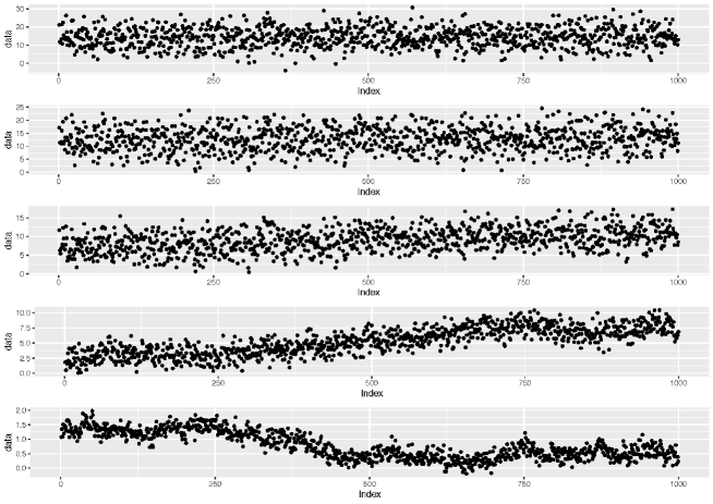
which implies that far away observations may be less similar, suggesting nonstationarity. Then we propose five simulation cases,
and , where the matrix . So, the is a stationary term. In Case 1, the data is generated from a highly nonstationary process and is a five dimensional vector consisting of independent draws from a uniform distribution. In Case 3, we weight the process half with a nonlinear term and half with a stationary term. In Case 5, we only have a stationary term. So the data is rough in Case 1 and gradually becomes smoother as we consider other cases. We show examples of the data in Figure (1).
We generate 1,000 observations over this one-dimensional domain for each case. For Case 2 to Case 4, is set to be equal to the sample variance of the elements in the vector . We fixed . SNR is defined to be
so that
Each SNR has five different cases as we mention above. In practice, we often do not observe all the useful covariates. Thus, when implementing methods for spatial prediction, we only use , which removes .
In our model, the 20-dimensional vector was chosen to consist of Gaussian radial basis functions over equally spaced knots. That is, , where
and are the equally-spaced knots points over , and is equal to 1.5 times the median of non-zero distances between the points in . We set the spectral density equal to
In Table (1), we provide the root mean squared prediction error (RMSPE) of each model for the data in the first row in Figure (1). The RMSPE is defined as
| (6) |
where is the posterior mean from fitting the each model. Here we see that our method (referred to as the Expanded Spectral Density (ESD) method) clearly outperform NNGP and the Vecchia approximation. Our model performs well in terms of estimation as well. Using the data in the first row of Figure (1), and a half-t prior for , we have a posterior mean of equal to 5.79 and highest posterior density interval, (2.68, 9.96). The true value is 4.813, which is contained in the interval.
| Method | RMSPE |
|---|---|
| ESD | 1.94 |
| NNGP | 3.24 |
| Vecchia Approximation | 3.05 |
4.1 Comparisons Over Multiple Replicates
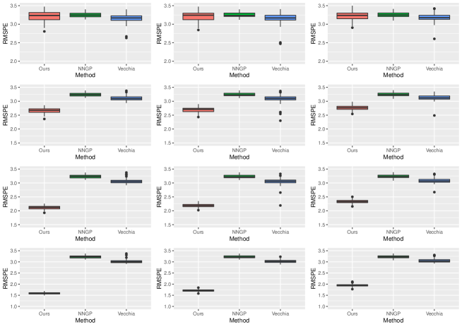
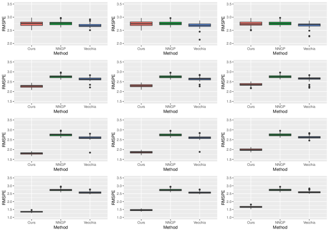
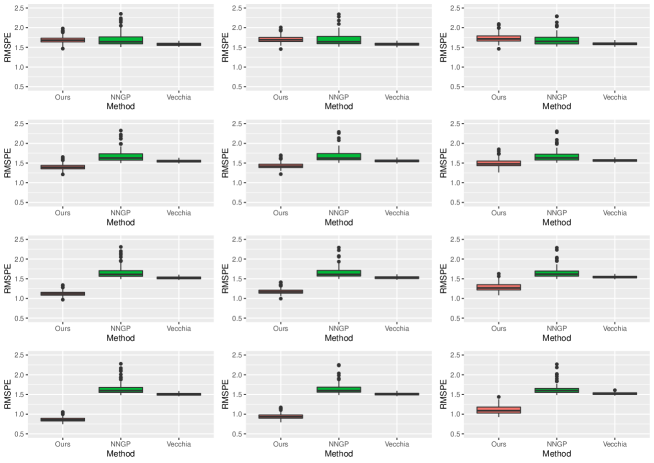
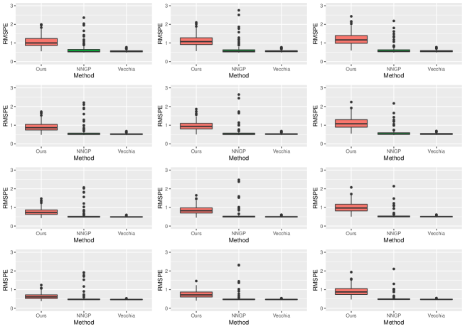
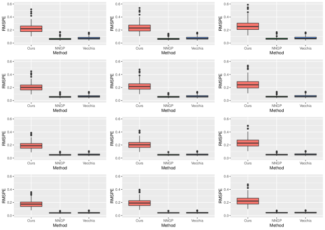
To implement NNGP, we use 15 nearest neighbors which is consistent with what is suggested in Datta et al., (2016a). For the general Vecchia approximation, we use 15 nearest neighbors which is the same as NNGP. We also use the R-package spNNGP (AO Finley,, 2017) and GpGp (Guinness and Katzfuss,, 2018). We record the performance (in terms of RMSPE) over the signal noise ratio (SNR) and the proportion of missing in the datasets for each case. The results are show in Figure (2) to Figure (6) for Case 1 to Case 5, respectively. For each figure, the first row is for SNR equal 2, the second row if for SNR equal 3, the third row is for SNR equal 5 and the fourth row is for SNR equal 10. For each row, the left plot has 5% of the data missing, the middle plot has 10% of the data missing and the right plot has 20% of the data missing. The boxplot is computed over 100 independent replicates of the one thousand dimensional dataset. We compare each simulation with NNGP and the general Vecchia approximation.
For both Case 1 and Case 2, we find that our method outperforms the NNGP and the general Vecchia approximation when SNR equals 3, 5 and 10. However, we have a similar result with NNGP and perform slight worse than general Vecchia approximation when SNR=2. In Case 3, we find that our method outperforms the NNGP and general Vecchia approximation when SNR equals 5 and 10, and only slightly outperforms NNGP and general Vecchia approximation when SNR=3. Additionally, ESD performs slightly worse than general Vecchia approximation when SNR=2 and we are in Case 3. In Case 4, we find that general Vecchia approximation outperforms our method, and our method outperforms than NNGP in a few replicates. In Case 5, the stationary case, general Vecchia approximation and NNGP outperform our method, which is not surprising considering that our method is derived for nonstationary processes. Based on the results, we believe our model performs well in highly nonlinear setting with moderate to high signal-to-noise ratios. However, we find the RMSPE is worse than NNGP and general Vecchia approximation when as the process becomes smoother.
5 Real Data Application
5.1 Ozone Data Application: Data Description
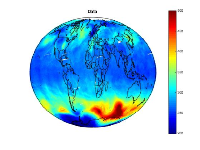
As an illustration, we analyze the ozone dataset used in Cressie and Johannesson, (2008), which has become a benchmark dataset in the spatial statistics literature (Zhang et al.,, 2018). This dataset consists of values of total column ozone (TCO) in Dobson units (see Figure (7) for a plot of the data). The dataset was obtained through a Dobson spectrophotometer on board the Nimbus-7 polar orbiting satellite on October 1st, 1988. For details on how these data were collected see Cressie and Johannesson, (2008). This dataset is made publically available by the Centre for Environmental Informatics at the University of Wollongong’s National Institute for Applied Statistics Research Australia (https://hpc.niasra.uow.edu.au/ckan/).
 |
5.2 Analysis
We present an analysis of the ozone dataset using ESD. We partition the data into a training set and a prediction set. We randomly generated three different 5% missing at random datasets for evaluating the prediction performance of all methods. A total of 5,000 MCMC iterations of the Gibbs sampler in Algorithm 1 were used. The first 1,000 iterations were treated as a burn-in. We informally check trace plots for convergence, and no lack of convergence was detected. Since d=2, is an dimensional matrix, which we denote with , where is an r-dimensional vector, i=1,2. Using the R-package FRK, we choose 92, 364 and 591 equally-spaced bisquare basis functions, which defines a 92, 364 and 591-dimensional vector (Zammit-Mangion and Cressie,, 2017). Then, we set , and we take . This choice of isolates the effect of the latitude and longitude on the non-stationarity of the process. The covariates are defined to be .
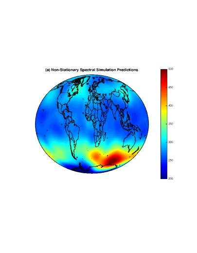
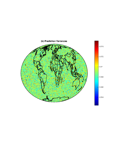
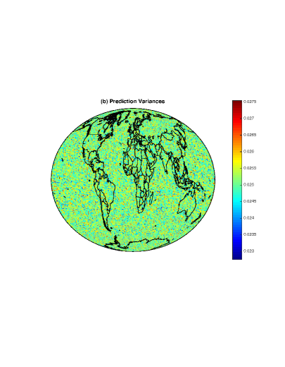
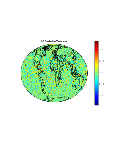
Figure (8) displays the prediction and prediction variances using non-stationary spectral simulation. Upon comparison of Figure (7) to Figure (8a),Figure (9a) and Figure (10a) , we see that we obtain small in-sample error. Additionally, Figure (8b), Figure (9b) and Figure (10b) shows that our prediction error is relatively constant over the globe. We randomly select 5% of the total observations to act as a validation dataset, and compute the root mean squared prediction error (RMSPE). Specifically, we compute the average square distance between the validation data and its corresponding prediction, and then we take the square root. RMSPE for our method is around 16.55, 9.86 and 7.52 for 92, 364 and 591 basis functions, respectively (see Table 2). We also computed the RMSPE for the fixed rank kriging method as implemented through the R-package FRK (Zammit-Mangion and Cressie,, 2017). The FRK predictor is based on and uses as its basis set. The RMSPE for FRK is approximately 76.41, and hence, we outperform the FRK predictor in terms of RMSPE. We do compare to other methods as well. In Zhang et al., (2018) paper, they compare the Smoothed Full-Scale Approximation (SFSA), Full-Scale Approximation using a block modulating function (FSAB) (Sang and Huang,, 2012), NNGP, and a local Gaussian process method with adaptive local designs (LaGP) (Gramacy and Apley,, 2015). Their results show that the RMSPE for SFSA, NNGP and FSAB are all around 27, and the RMSPE for LaGP is around 38. Thus, our method also outperforms these methods in terms of RMSPE. However, the general Vecchia approximation has a slightly better result. With RMSPE equal to roughly 5, which is smaller than our RMSPE of 7.52. This consistent with our simulation results that showed that in smoother nonstationary settings the general Vecchia approximation performs similar or better than ESD.
We also include the computation times in Table (3). Our method is less competitive. Although we avoid storing and inverting a high dimensional covariance matrix, we require nested loops, which can be computationally intensive (i.e., a loop in the Gibbs sampler and a loop over in Theorem 2). However, we are able to produce spatial predictions.
|

|

|
| Total size of basis function | RMSPE |
|---|---|
| 92 | 16.55 |
| 364 | 9.86 |
| 591 | 7.52 |
| Method | Number of basis function | Time (seconds) |
|---|---|---|
| ESD | 92 | 13925 |
| 364 | 111685 | |
| 591 | 273024 | |
| Vecchia Approximation | - | 200 |
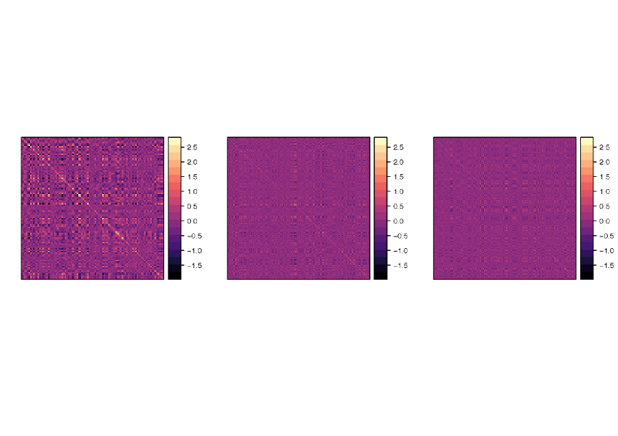
In terms of inference on parameters, we are particularly interested in . This is because when is zero we obtain a stationary process (see Theorem 1). In Figure (11) we plot the posterior covariance matrix. As the increases, we see the variances and covariances appear to be close to zero suggesting that is close to zero. This suggests that the process is smooth, which is consistent with our previous results. However, several credible intervals for elements of do not contain zero, which suggests that nonstationarity is present in this dataset.
 |
6 Discussion
Bayesian analysis of big Gaussian spatial data is a challenging and important problem. We propose a Bayesian approach using non-stationary spectral simulation. To develop non-stationary spectral simulation we combine Bochner’s theorem with dimension expansion (Perrin and Meiring,, 2003), and apply Mejía and Rodríguez-Iturbe, (1974)’s spectral simulation method. The advantage is that no large matrix inversion or storage is needed to approximately simulate a non-stationary full-rank Gaussian process. Additionally, the proposed method is extremely broad, since every positive definite non-stationary covariance function can be written according to (3).
In Section 4, the simulation study is used to show a scenario where our approach outperforms the nearest neighbor Gaussian process (NNGP; Datta et al.,, 2016a) model and Vecchia approximation (Katzfuss and Guinness,, 2017). We generate data that is different from our model, and we find our method has better result in different scenarios based on how nonlinear the process is. In Section 5, we analyze the total column ozone dataset from Cressie and Johannesson, (2008). We obtain predictions that have small in-sample error, and outperforms fixed rank kriging (FRK), SFSA, FSAB, NNGP, and LaGP in terms of out-of-sample error. The Vecchia approximation has a slightly better RMSPE. Additionally, our framework allows one to perform inference on the presence of nonstationarity.
Environmental studies are often based on high-dimensional spatial Gaussian datasets with complex patterns of non-stationarity. Several studies focus on simplifying matrix valued operations and storage (Higdon et al.,, 1999; Paciorek and Schervish,, 2006; Cressie and Johannesson,, 2008; Banerjee et al.,, 2008; Lindgren et al.,, 2011; Nychka et al.,, 2015). Thus, our “matrix free” approach offers a unique solution to this important problem.
Acknowledgments
Jonathan Bradley’s research was partially supported by the U.S. National Science Foundation (NSF) grant SES-1853099.
Appendix A: Proofs
Proof of Theorem 1:
It follows from Perrin and Meiring, (2003) that for every non-stationary positive definite function C and every pair of locations and there exists a and such that , where is a stationary covariogram. Let be the function that maps a generic location to it’s corresponding expanded dimension .
It follows from Bochner’s theorem (Bochner,, 1959) that is positive definite (and equivalently so is ) if and only if
This completes the result.
Proof of Theorem 2:
We have that,
since . Also,
since is a stationary covariogram it follow from Cressie, (1993, pg. 204) that converges to a Gaussian process.
Appendix B: Full Conditional Distributions
In this section, we derive the full conditional distribution of our parameters and random effects, which we use within the Gibbs sampler outlined in Algorithm 1.
-
1.
The full conditional distribution for is
Thus, , where and , .
-
2.
First, we sample using non-stationary spectral simulation. Then the full-conditional distribution is
where . Then,
This gives
where , and .
-
3.
The approximated full conditional distribution for is given by
where recall is a function of . We use Metropolis-Hasting to sample and we use a multivariate normal distribution for the proposal distribution.
-
4.
For , we use a Inverse Gamma prior distribution,
which is an inverse gamma distribution with shape parameter and scale parameter .
-
5.
The full conditional distribution of is easily obtained and given by,
which is an inverse gamma distribution with shape parameter and scale parameter .
-
6.
The full conditional distribution of is easily obtained and given by,
which is an inverse gamma distribution with shape parameter and scale parameter .
-
7.
The prior for is , and the full conditional distribution for follows that,
-
8.
The full conditional distribution of is easily obtained and given by,
which is an inverse gamma distribution with shape parameter and scale parameter .
-
9.
The full conditional distribution of is easily obtained and given by,
which is an inverse gamma distribution with shape parameter and scale parameter .
References
- Anderes and Stein, (2011) Anderes, E. B. and Stein, M. L. (2011). “Local likelihood estimation for nonstationary random fields.” Journal of Multivariate Analysis, 102, 3, 506–520.
- AO Finley, (2017) AO Finley, A Datta, S. B. (2017). “Package ‘spNNGP’.” https://cran.r-project.org/web/packages/spNNGP/index.html.
- Banerjee et al., (2015) Banerjee, S., Carlin, B. P., and Gelfand, A. E. (2015). Hierarchical modeling and analysis for spatial data. Boca Raton, FL, CRC Press.
- Banerjee et al., (2008) Banerjee, S., Gelfand, A. E., Finley, A. O., and Sang, H. (2008). “Gaussian predictive process models for large spatial data sets.” Journal of the Royal Statistical Society: Series B (Statistical Methodology), 70, 4, 825–848.
- Bochner, (1959) Bochner, S. (1959). Lectures on Fourier Integrals. No. 42. Princeton University Press.
- Bornn et al., (2017) Bornn, L., Pillai, N. S., Smith, A., and Woodard, D. (2017). “The use of a single pseudo-sample in approximate Bayesian computation.” Statistics and Computing, 27, 3, 583–590.
- Bornn et al., (2012) Bornn, L., Shaddick, G., and Zidek, J. V. (2012). “Modeling nonstationary processes through dimension expansion.” Journal of the American Statistical Association, 107, 497, 281–289.
- Bradley et al., (2011) Bradley, J. R., Cressie, N., and Shi, T. (2011). “Selection of rank and basis functions in the Spatial Random Effects model.” In Proceedings of the 2011 Joint Statistical Meetings, 3393–3406. Alexandria, VA: American Statistical Association.
- Bradley et al., (2016) Bradley, J. R., Cressie, N., Shi, T., et al. (2016). “A comparison of spatial predictors when datasets could be very large.” Statistics Surveys, 10, 100–131.
- Bradley et al., (2018) Bradley, J. R., Wikle, C. K., and Holan, S. H. (2018). “Hierarchical Models for Spatial Data with Errors that are Correlated with the Latent Process.”
- Castruccio and Guinness, (2017) Castruccio, S. and Guinness, J. (2017). “An evolutionary spectrum approach to incorporate large-scale geographical descriptors on global processes.” Journal of the Royal Statistical Society: Series C (Applied Statistics), 66, 2, 329–344.
- Cressie and Johannesson, (2008) Cressie, N. and Johannesson, G. (2008). “Fixed rank kriging for very large spatial data sets.” Journal of the Royal Statistical Society: Series B (Statistical Methodology), 70, 1, 209–226.
- Cressie, (1993) Cressie, N. A. (1993). “Statistics for spatial data.”
- Cressie and Wikle, (2011) Cressie, N. A. and Wikle, C. (2011). “Statistics for Spatio-Temporal Data.”
- Datta et al., (2016a) Datta, A., Banerjee, S., Finley, A. O., and Gelfand, A. E. (2016a). “Hierarchical nearest-neighbor Gaussian process models for large geostatistical datasets.” Journal of the American Statistical Association, 111, 514, 800–812.
- Datta et al., (2016b) — (2016b). “On nearest-neighbor Gaussian process models for massive spatial data.” Wiley Interdisciplinary Reviews: Computational Statistics, 8, 5, 162–171.
- Finley et al., (2013) Finley, A. O., Banerjee, S., and Gelfand, A. E. (2013). “spBayes for large univariate and multivariate point-referenced spatio-temporal data models.” Journal of Statistical Software.
- Friedman et al., (1991) Friedman, J. H. et al. (1991). “Multivariate adaptive regression splines.” The annals of statistics, 19, 1, 1–67.
- Fuentes, (2002) Fuentes, M. (2002). “Spectral methods for nonstationary spatial processes.” Biometrika, 89, 1, 197–210.
- Fuentes et al., (2008) Fuentes, M., Chen, L., and Davis, J. M. (2008). “A class of nonseparable and nonstationary spatial temporal covariance functions.” Environmetrics, 19, 5, 487–507.
- Fuentes and Smith, (2001) Fuentes, M. and Smith, R. L. (2001). “A new class of nonstationary spatial models.” Tech. rep., unpublished manuscript, available at www.stat.ncsu.edu/information/library/papers/nonstat.ps.
- Fuglstad et al., (2015) Fuglstad, G.-A., Simpson, D., Lindgren, F., and Rue, H. (2015). “Interpretable priors for hyperparameters for Gaussian random fields.” arXiv preprint arXiv:1503.00256.
- Gelfand, (2000) Gelfand, A. E. (2000). “Gibbs sampling.” Journal of the American statistical Association, 95, 452, 1300–1304.
- Gelfand and Smith, (1990) Gelfand, A. E. and Smith, A. F. (1990). “Sampling-based approaches to calculating marginal densities.” Journal of the American statistical association, 85, 410, 398–409.
- Gelman, (2006) Gelman, A. (2006). “Prior distributions for variance parameters in hierarchical models (comment on article by Browne and Draper).” Bayesian analysis, 1, 3, 515–534.
- Gramacy and Apley, (2015) Gramacy, R. B. and Apley, D. W. (2015). “Local Gaussian process approximation for large computer experiments.” Journal of Computational and Graphical Statistics, 24, 2, 561–578.
- Guinness and Katzfuss, (2018) Guinness, J. and Katzfuss, M. (2018). “GpGp: Fast Gaussian Process Computation Using Vecchia’s Approximation.” R package version 0.1. 0.
- Guinness and Stein, (2013) Guinness, J. and Stein, M. L. (2013). “Interpolation of nonstationary high frequency spatial–temporal temperature data.” The Annals of Applied Statistics, 7, 3, 1684–1708.
- Hastings, (1970) Hastings, W. K. (1970). “Monte Carlo sampling methods using Markov chains and their applications.” Biometrika, 57, 1, 97–109.
- Heaton et al., (2017) Heaton, M. J., Datta, A., Finley, A., Furrer, R., Guhaniyogi, R., Gerber, F., Gramacy, R. B., Hammerling, D., Katzfuss, M., Lindgren, F., et al. (2017). “Methods for Analyzing Large Spatial Data: A Review and Comparison.” arXiv preprint arXiv:1710.05013.
- Higdon, (1998) Higdon, D. (1998). “A process-convolution approach to modelling temperatures in the North Atlantic Ocean.” Environmental and Ecological Statistics, 5, 2, 173–190.
- Higdon et al., (1999) Higdon, D., Swall, J., and Kern, J. (1999). “Non-stationary spatial modeling.” Bayesian statistics, 6, 1, 761–768.
- Horrell and Stein, (2017) Horrell, M. T. and Stein, M. L. (2017). “Half-spectral space–time covariance models.” Spatial Statistics, 19, 90–100.
- Im et al., (2007) Im, H. K., Stein, M. L., and Zhu, Z. (2007). “Semiparametric estimation of spectral density with irregular observations.” Journal of the American Statistical Association, 102, 478, 726–735.
- Kalkhan, (2011) Kalkhan, M. A. (2011). Spatial statistics: geospatial information modeling and thematic mapping. Boca Raton, FL, CRC Press.
- Kang and Cressie, (2011) Kang, E. L. and Cressie, N. (2011). “Bayesian inference for the Spatial Random Effects model.” Journal of the American Statistical Association, 106, 972 – 983.
- Katzfuss, (2013) Katzfuss, M. (2013). “Bayesian nonstationary spatial modeling for very large datasets.” Environmetrics, 24, 3, 189–200.
- Katzfuss, (2017) — (2017). “A multi-resolution approximation for massive spatial datasets.” Journal of the American Statistical Association, 112, 517, 201–214.
- Katzfuss and Guinness, (2017) Katzfuss, M. and Guinness, J. (2017). “A general framework for Vecchia approximations of Gaussian processes.” arXiv preprint arXiv:1708.06302.
- Katzfuss et al., (2018) Katzfuss, M., Guinness, J., and Gong, W. (2018). “Vecchia approximations of Gaussian-process predictions.” arXiv preprint arXiv:1805.03309.
- Kleiber and Nychka, (2012) Kleiber, W. and Nychka, D. (2012). “Nonstationary modeling for multivariate spatial processes.” Journal of Multivariate Analysis, 112, 76–91.
- Lindgren et al., (2011) Lindgren, F., Rue, H., and Lindström, J. (2011). “An explicit link between Gaussian fields and Gaussian Markov random fields: the stochastic partial differential equation approach.” Journal of the Royal Statistical Society: Series B (Statistical Methodology), 73, 4, 423–498.
- Liu, (1994) Liu, J. S. (1994). “The collapsed Gibbs sampler in Bayesian computations with applications to a gene regulation problem.” Journal of the American Statistical Association, 89, 427, 958–966.
- Martin, (1982) Martin, W. (1982). “Time-frequency analysis of random signals.” In Acoustics, Speech, and Signal Processing, IEEE International Conference on ICASSP’82., vol. 7, 1325–1328. IEEE.
- Mejía and Rodríguez-Iturbe, (1974) Mejía, J. M. and Rodríguez-Iturbe, I. (1974). “On the synthesis of random field sampling from the spectrum: An application to the generation of hydrologic spatial processes.” Water Resources Research, 10, 4, 705–711.
- Neal, (2003) Neal, R. M. (2003). “Slice sampling.” Annals of statistics, 705–741.
- Neto et al., (2014) Neto, J. H. V., Schmidt, A. M., and Guttorp, P. (2014). “Accounting for spatially varying directional effects in spatial covariance structures.” Journal of the Royal Statistical Society: Series C (Applied Statistics), 63, 1, 103–122.
- Nychka et al., (2015) Nychka, D., Bandyopadhyay, S., Hammerling, D., Lindgren, F., and Sain, S. (2015). “A multiresolution Gaussian process model for the analysis of large spatial datasets.” Journal of Computational and Graphical Statistics, 24, 2, 579–599.
- Nychka, (2001) Nychka, D. W. (2001). “Spatial process estimates as smoothers.” In Smoothing and Regression: Approaches, Computation and Applications, rev. ed, ed. M. G. Schmiek, 393–424. New York, NY: Wiley.
- Paciorek and Schervish, (2006) Paciorek, C. J. and Schervish, M. J. (2006). “Spatial modelling using a new class of nonstationary covariance functions.” Environmetrics, 17, 5, 483–506.
- Perrin and Meiring, (2003) Perrin, O. and Meiring, W. (2003). “Nonstationarity in ℝn is second-order stationarity in ℝ2n.” Journal of applied probability, 40, 3, 815–820.
- Priestley, (1965) Priestley, M. B. (1965). “Evolutionary spectra and non-stationary processes.” Journal of the Royal Statistical Society. Series B (Methodological), 204–237.
- Prokhorov, (1956) Prokhorov, Y. V. (1956). “Convergence of random processes and limit theorems in probability theory.” Theory of Probability & Its Applications, 1, 2, 157–214.
- Resnick, (2013) Resnick, S. I. (2013). A probability path. Springer Science & Business Media.
- Risser, (2016) Risser, M. D. (2016). “Nonstationary Spatial Modeling, with Emphasis on Process Convolution and Covariate-Driven Approaches.” arXiv preprint arXiv:1610.02447.
- Robert, (2004) Robert, C. P. (2004). Monte carlo methods. Wiley Online Library.
- Sampson and Guttorp, (1992) Sampson, P. D. and Guttorp, P. (1992). “Nonparametric estimation of nonstationary spatial covariance structure.” Journal of the American Statistical Association, 87, 417, 108–119.
- Sang and Huang, (2012) Sang, H. and Huang, J. Z. (2012). “A full scale approximation of covariance functions for large spatial data sets.” Journal of the Royal Statistical Society: Series B (Statistical Methodology), 74, 1, 111–132.
- Sayeed and Jones, (1995) Sayeed, A. M. and Jones, D. L. (1995). “Optimal kernels for nonstationary spectral estimation.” IEEE Transactions on Signal Processing, 43, 2, 478–491.
- Schmidt and O’Hagan, (2003) Schmidt, A. M. and O’Hagan, A. (2003). “Bayesian inference for non-stationary spatial covariance structure via spatial deformations.” Journal of the Royal Statistical Society: Series B (Statistical Methodology), 65, 3, 743–758.
- Shand and Li, (2017) Shand, L. and Li, B. (2017). “Modeling nonstationarity in space and time.” Biometrics.
- Simpson et al., (2017) Simpson, D., Rue, H., Riebler, A., Martins, T. G., Sørbye, S. H., et al. (2017). “Penalising model component complexity: A principled, practical approach to constructing priors.” Statistical Science, 32, 1, 1–28.
- Spiegelhalter et al., (2002) Spiegelhalter, D. J., Best, N. G., Carlin, B. P., and Van Der Linde, A. (2002). “Bayesian measures of model complexity and fit.” Journal of the Royal Statistical Society: Series B (Statistical Methodology), 64, 4, 583–639.
- Stein et al., (2006) Stein, A., van der Meer, F. D., and Gorte, B. (2006). Spatial statistics for remote sensing, vol. 1. Springer Science & Business Media.
- Stein, (1999) Stein, M. L. (1999). Statistical Interpolation of spatial Data: Some Theory for Kriging. Place Springer.
- Stein, (2012) — (2012). Interpolation of spatial data: some theory for kriging. Springer Science & Business Media.
- Stein, (2014) — (2014). “Limitations on low rank approximations for covariance matrices of spatial data.” Spatial Statistics, 8, 1–19.
- Stein, (2015) — (2015). “When does the screening effect not hold?” Spatial Statistics, 11, 65–80.
- Stein et al., (2004) Stein, M. L., Chi, Z., and Welty, L. J. (2004). “Approximating likelihoods for large spatial data sets.” Journal of the Royal Statistical Society: Series B (Statistical Methodology), 66, 2, 275–296.
- Tierney, (1994) Tierney, L. (1994). “Markov chains for exploring posterior distributions.” the Annals of Statistics, 1701–1728.
- Tzeng and Huang, (2017) Tzeng, S. and Huang, H.-C. (2017). “Resolution adaptive fixed rank kriging.” Technometrics, DOI: 10.1080/00401706.2017.1345701.
- Zammit-Mangion and Cressie, (2017) Zammit-Mangion, A. and Cressie, N. (2017). “FRK: An R Package for Spatial and Spatio-Temporal Prediction with Large Datasets.” arXiv preprint arXiv:1705.08105.
- Zhang et al., (2018) Zhang, B., Sang, H., and Huang, J. Z. (2018). “Smoothed full-scale approximation of Gaussian process models for computation of large spatial datasets.” Statistica Sinica, accepted.
- Ziemke et al., (2005) Ziemke, J., Chandra, S., and Bhartia, P. (2005). “A 25-year data record of atmospheric ozone in the Pacific from Total Ozone Mapping Spectrometer (TOMS) cloud slicing: Implications for ozone trends in the stratosphere and troposphere.” Journal of Geophysical Research: Atmospheres, 110, D15.